Abstract

Prior-Fitted Networks (PFNs) have recently been proposed to efficiently perform tabular classification tasks. Although they achieve good performance on small datasets, they encounter limitations with larger datasets. These limitations include significant memory consumption and increased computational complexity, primarily due to the impracticality of incorporating all training samples as inputs within these networks. To address these challenges, we investigate the fitting assumption for PFNs and input samples. Building on this understanding, we propose BoostPFN designed to enhance the performance of these networks, especially for large-scale datasets. We also theoretically validate the convergence of BoostPFN and our empirical results demonstrate that the BoostPFN method can outperform standard PFNs with the same size of training samples in large datasets and achieve a significant acceleration in training times compared to other established baselines in the field, including widely-used Gradient Boosting Decision Trees (GBDTs), deep learning methods and AutoML systems. High performance is maintained for up to 50x of the pre-training size of PFNs, substantially extending the limit of training samples. Through this work, we address the challenges of efficiently handling large datasets via PFN-based models, paving the way for faster and more effective tabular data classification training and prediction process. Code is available at https://github.com/yxzwang/BoostPFN.

1 Introduction

Tabular datasets are increasingly garnering attention in various practical applications across fields such as finance [9], healthcare [12], and scientific research [10], among others [3, 45, 46, 47]. As we continue to amass larger and more complex datasets, the need for efficient and effective methods of data analysis becomes ever more critical. Traditional approaches often fall short due to prohibitively long training times when dealing with large datasets. This limitation not only hampers the speed of data processing but also impacts the overall feasibility of utilizing large-scale tabular data in time-sensitive scenarios [10].

Recently, there has been a significant shift towards exploring novel methodologies that can overcome the limitations of traditional data processing techniques. One such promising development is the advent of the in-context learning method known as Prior-fitted Networks (PFNs) [33]. This innovative approach is capable of making predictions without the need for training on the training set, instead utilizing training data points as input tokens to the model architecture, thereby offering a much faster training and prediction process compared to conventional methods. The outstanding model in Prior-fitted Networks: TabPFN [21], uses a Transformer as the model architecture. Therefore, the primary issue with TabPFN on large datasets lies in the scalability of the Transformer: when applied to large datasets, it becomes impractical due to excessive memory consumption and computational complexity. The computational complexity of the Transformer increase quadratically with input length, which, for TabPFN, corresponds to the size of the training dataset. Despite these challenges, TabPFN’s ability to rapidly process large tabular datasets remains a compelling feature, urging us to find a way to apply it to large datasets.

Table 1: Comparison of BoostPFN with GBDTs, Deep Learning (D.L.) methods and TabPFN.

Models	Strong Performance with Limited Training Samples	Training Efficiency	Large Datasets
GBDTs	✗	✗	✓
D.L.	✗	✗	✓
TabPFN	✓	✓	✗
BoostPFN	✓	✓	✓

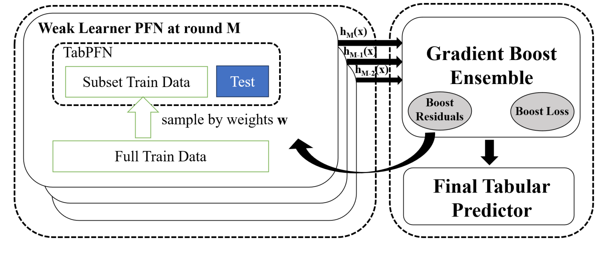
Figure 1: Overview of BoostPFN. Each PFN with a subset of train data is viewed as a weak learner $h_{M}(x)$ at round $M$. While adding new weak learners into the ensemble, new weak learner is governed by updating new sampling weights with the boosting residuals from the existing ensemble.

In this paper, we introduce a way to treat PFN as a type of "weak" learner in the gradient boosting process, achieved through the Fitting Assumption 4.1. We then propose BoostPFN as an extension of Gradient Boosting [14] for ensembling these PFNs, as illustrated in Figure 1. We propose three updating methods based on the Fitting Assumption, including the AdaBoost updating, which allows our method to be viewed as a natural extension of the well-known boosting method AdaBoost [19]. These methods explore how ensemble learning techniques can be integrated with PFNs to create a more robust prediction model. We delve into both the theoretical and empirical validation of BoostPFN and demonstrate that our proposed methods not only achieve high performance but also maintain the efficiency in training that is critical for handling large-scale tabular datasets, compared to GBDTs and other deep learning methods that are trained explicitly. We compare BoostPFN with other types of models in Table 1. Our contributions are as follows:

• TabPFN is designed for fast training on tabular classification tasks but cannot handle large datasets, while BoostPFN extends the training dataset size and retains high performance, accommodating up to 50x the pre-training size of TabPFN. Importantly, even when limited by TabPFN’s pre-training size of 1024, which struggles to yield relatively good results compared to other models, our method paves the way for extending any new or improved PFN with a larger pre-training size and better training data.

• We delve into the theoretical analysis of BoostPFN, showing that it is a type of Randomized Gradient Boosting Machine with a convergence guarantee. Empirical results also demonstrate the convergence of boosting loss on both the training and test sets when overfitting does not occur.

• We conduct extensive experiments on datasets of varying sizes, from small to large, to assess the performance of BoostPFN, highlighting its efficacy and scalability.

2 Preliminaries

Posterior Predictive Distribution. The Posterior Predictive Distribution (PPD) is a concept in Bayesian statistics that combines the information from both the observed data and the posterior distribution of the model parameters. It is a predictive distribution for future observations based on the updated beliefs about the model parameters after incorporating the observed data.

$$p(y|x,D)\propto\int_{\Phi}p(y|x,\phi)p(D|\phi)p(\phi)d\phi.$$ (1)

PFNs and Architecture. PFNs are proposed in [33, 21] to approximate the Posterior Predictive Distribution (PPD) for supervised learning. For a test sample $x_{test}$ and train datasets $D:={(x_{i},y_{i})}_{i\in\{1,\dots,n\}}$, the prediction of TabPFN [21] can be written as

$$p(\hat{y}_{test})=q_{\theta}(\hat{y}_{test}|x_{text},D_{train}),$$ (2)

where $\theta$ are the parameters of TabPFN. The architecture of TabPFN is a Transformer without positional embeddings. Training samples and test samples are concatenated together and taken as the input of Transformer. Probabilities for each class are given by Transformer as output.

Gradient Boosting. Gradient Boosting [14] is a powerful machine learning technique that constructs a predictive model $F_{m}(x)$ in the form of an ensemble of weak predictive models (commonly decision trees) at iteration $m$,

$$F_{m}(x)=F_{m-1}(x)+\gamma_{m}h_{m}(x),$$ (3)

where $h_{m}(x)$ is a weak learner selected from the candidate learner space $\mathcal{H}$ and $\gamma_{m}$ is the learning rate learned by line search. The $h_{m}(x)$ is selected to fit the residual errors $r_{m}=-\left[\frac{\partial\ell(y,F_{m-1}(x))}{\partial F_{m-1}(x_{i})}\right]$ of the prior models,

$$h_{m}=\text{args}\min_{h\in\mathcal{H}}\sum_{i=1}^{|D_{train}|}||r_{m}[i]-h(x_{i})||_{2}^{2},$$ (4)

where $r_{m}[i]$ is the $i$th value of vector $r_{m}$.

3 PFN Scalability Challenges

Long-range Transformers. While the Transformer is the backbone of TabPFN, it faces challenges with large datasets because TabPFN considers all training samples at once. There are Transformer variants [18, 8, 2, 50, 48] that enable long-range inputs and show promising results compared to the vanilla Transformer with thousands of input tokens. However, for larger datasets with more training samples, the capability of handling thousands of input tokens is merely a drop in the bucket, and pre-training inevitably requires substantial time. Although one direction is to develop more efficient Transformer architectures, we focus on the alternative direction: applying a trained PFN to larger datasets.

Sampling Methods. A straightforward approach is to sample a small portion of training samples as the input training datasets, which is common for Transformers. In Natural Language Processing, training datasets are retrieved by a Retriever [37, 38, 35, 26, 51, 28, 24, 49, 40, 44, 30] that considers the relationship between the test sample and candidate samples. However, retriever-based methods retrieve training samples differently for each test sample, making implementation challenging when the number of test samples is large. Additionally, retrieving training samples from a vast number of candidates is time-consuming, and results are not guaranteed because existing retrievers can only accept thousands of candidates. Therefore, we opt to use simple sampling for training sample selection. However, this simple approach is very heuristic and may not yield good performance. To improve performance, we can employ ensemble methods. One of the simplest ensemble methods is Bagging [6], which samples multiple times and averages the predictions. We include this as our ensemble baseline method. For better performance, we will next introduce our method of scaling PFNs through boosting.

4 Scaling PFNs through Boosting

We propose a gradient boosting method for PFNs called BoostPFN. In the normal procedure of gradient boosting discussed in Section 2, an essential step is to fit a new weak learner based on training residuals, as shown in Eq. 4. For traditional weak learners, such as decision trees, this is easy to implement. However, for PFNs, there is no existing method to fit a new PFN while keeping the parameters of the Transformer architecture fixed. Optimizing the parameters of a PFN using gradient methods is time-consuming and undermines the primary advantage of PFNs, which is their negligible training time. To maintain training efficiency and enable the fitting step, we first propose learnable sampling optimization for PFNs. Since the input datasets are a crucial part of predicting the target sample, optimizing the input dataset can also enhance prediction accuracy. For normalized sampling weights $w$, a specified PFN $q_{\theta}$, and a test sample $x_{test}$, a PFN with a sampled input dataset is defined as

$$q_{(\theta,w)}(y|x_{test},D)=q_{\theta}(y|x_{test},D_{w}^{z}),$$ (5)

where $D$ is the full training set and $D_{w}^{z}$ is the sampled input dataset generated by weights $w\in\mathbf{R}^{|D|}$ and sampling size $z\in(0,|D|]$ which determines the sampled training set size $|D_{w}^{z}|=z$.

4.1 Optimizing Input Datasets

We first describe how we optimize the input dataset by updating $w$ using pseudo-residuals, similar to the approach in gradient boosting.

Assumption 4.1.

Given a sample $(x_{i},y_{i})$, and any training set $\tilde{D}$, the probability of predicting the right class $y_{i}$ on $x_{i}$ be

$$q_{\theta}(y_{i}|x_{i},\tilde{D}\cup\{(x_{i},y_{i})\})>$$ (6)

$$\max\Big{[}q_{\theta}(y_{i}|x_{i},\tilde{D}),q_{\theta}(y_{i}|x_{i},\tilde{D}\cup\{(x_{j},y_{j})\})\Big{]},$$

Assumption 4.1 can be explained simply: adding the target sample or replacing one sample in the training set with the target sample will improve prediction performance. This seems straightforward for a GP (Gaussian Process) [39], as fitting a GP to a single observation sharpens the posterior predictive distribution as it increases. However, PFNs are implemented in practice using a pretrained Transformer architecture, which does not inherently behave like a GP, and no such experiments have been conducted before. Therefore, we also perform experiments to empirically validate this assumption, as described in Section 7.1.

With this assumption, we can propose a simple idea: increasing the sampling weight $w[i]$ for $D[i]$ improves the probability of sampling that target $i$, thereby increasing the expectation of correctly predicting the label. Although this is a complex condition in practice, we can analyze it in a simplified scenario, as shown in Section A.1. This motivates a straightforward approach for updating sampling weights in a given dataset. In the next section, we explain in detail how to update them in practice.

4.2 Updating Sampling Weights

In this section, we discuss how to update sampling weights. Like the fitting residuals of gradient boosting in Eq. 4, we also want our our updating methods to depend on the residuals $r_{m}=-\left[\frac{\partial\ell(y,F_{m-1}(x))}{\partial F_{m-1}(x_{i})}\right]$. However, there is no previous work on how to apply residuals in sampling weights updating. Starting by remembering that in the gradient descent, the absolute value of gradient goes to zero when the loss come to the optimal plain. We come up with a rule for updating sampling weights, that is to give the sample with larger absolute residual more weights in the next round. Then we propose three updating methods in this section.

ExpHadamard Updating. New weights are the hadamard products of this round’s weights and the exponential of the residual,

$$w_{m}=w_{m-1}\odot\text{exp}(|r_{m}|).$$ (7)

Hadamard Updating. New weights are the hadamard products of this round’s weights and the residual,

$$w_{m}=w_{m-1}\odot|r_{m}|.$$ (8)

AdaBoost Updating. Also, we adopt the updating in AdaBoost [19] given by

$$\epsilon_{m} =w_{m-1}\otimes\textbf{1}\{h_{m-1}(X[i])\neq Y[i]\}$$

$$\alpha_{m} =\text{log}\left(\frac{1-\epsilon_{m}}{\epsilon_{m}}\right)+\text{log}(K-1),$$ (9)

$$w_{m} =w_{m-1}\odot\text{exp}\left(\alpha_{m}\textbf{1}\{h_{m-1}(X[i])\neq Y[i]\}\right),$$

where $\epsilon_{m}$ is the summation of the sampling weights of samples that the last weak learner predicts wrong on and $K$ is the class number of targets. And we increase the weights for wrong samples and decrease the weights for right samples based on $\epsilon_{m}$. As an alternative, the $\gamma_{m}$ could also be replaced by $\alpha_{m}$ as in AdaBoost. In practice, we choose the $\gamma_{m}$ with better performances. Note that although there is no residuals in the AdaBoost Updating, $\epsilon_{m}$ can be seen as a kind of residual for a specified AdaBoost loss funciton $\ell_{AdaBoost}$ [20].

In practice, we view the updating method as a hyperparameter of BoostPFN and choose the best one for each dataset. The ablation over different updating methods are shown in Section 7.2.

4.3 BoostPFN

By combining the ingredients from above, with the the gradient boosting process discussed in Section 2, we arrive at our BoostPFN approach, the steps of which are summarized in Algorithm 1.

0: Training data $D=(X,Y)$, PFN model $q_{\theta}(y|x,D)$ , sampling weights $w$ for training samples, sampling size $z$, boosting round number $M$ and boosting loss $\ell$.

Output: BoostPFN predictor $F(x)$.

1: Initialize by $F_{0}=0$.

2: for $m$ = 1 to $M$ do

3:  Compute residual: $r_{m}=-\frac{\partial\ell(y,F_{m-1}(X))}{\partial F_{m-1}(X)}$.

4:  Update sampling weights $w_{m}=Update(w_{m-1},r_{m})$ via methods in Section 4.2.

5:  $w_{m}\leftarrow\text{{Normalize}}(w_{m})$.

6:  Do non-replacement sampling with $w_{m}$ to obtain a subset of training data $D_{w_{m}}^{z}$

7:  Select new weak learner $h_{m}(x)$ as the PFN model $q_{\theta}(y|x,D_{w_{m}}^{z})$.

8:  Line search for $\gamma_{m}$ by $\gamma_{m}=\arg\text{min}_{\gamma}\sum_{i=1}^{N_{t}}\ell(Y[i],F_{m-1}(X[i])+\gamma h_{m}(X[i])$ .

9:  Get new predictor $F_{m}(x)=F_{m-1}(x)+\gamma_{m}h_{m}(x).$

10: end for

11: return $F(x)=F_{M}(x)$

Algorithm 1 BoostPFN

5 Analysis of BoostPFN

5.1 Time Complexity

Table 2: Time Complexity for PFNs. We use $T_{i}$ to denote the inference time for TabPFN. $M$ is the round we use for bagging or boosting. $T_{B}$ is the time cost of boosting operations in each boosting round.

TabPFN	Bagging	BoostPFN
$T_{i}$	$MT_{i}$	$M(T_{i}+T_{B})$

We briefly show the time complexity in Table 2. We consider the complexity analysis in a scenario with limited resources. Specifically, given the hardware available, we cannot load the entire test set due to out-of-memory (OOM) issues. Note that even with a small number of training samples, the OOM problem can still occur if the test set is large enough. Therefore, in practice, we have to split the test set into $N_{test}$ batches, and the inference of one batch consumes all the available memory (which is possible for millions of test samples). In this scenerio, the time complexity of BoostPFN is close to the simple Bagging method except for the addtion of inevitable boosting operations, which is an acceptable solution for large datasets. Then we describe in detail those symbols.

TabPFN. One inference of TabPFN on a single batch costs $O(L^{2})$ time, where $L=|D_{m}|+B$ represents the input length, equal to the sum of the length of the sampled dataset $|D_{m}|$ and the batch size $B$. For one inference of TabPFN on the entire test set, we need $T_{i}$ time. If we consider the sampling time negligible, this is also the time complexity for sampling a training set and performing TabPFN inference on the whole test set, which can be further reduced to

$$T_{i} =O(N_{test}(|D_{m}|+B)^{2})$$ (10)

$$=O(N_{test}(|D_{m}|^{2}+B^{2}+2|D_{m}|B))$$

$$=O\left(\frac{|D_{m}|^{2}}{B}|D_{test}|+B|D_{test}|+2|D_{m}||D_{test}|)\right)$$

$$=O\left(\left(\frac{|D_{m}|^{2}}{B}+B+2|D_{m}|\right)|D_{test}|\right),$$

where we use the fact that $O(N_{test}B)=O(|D_{test}|)$.

Bagging. As an easy ensemble method mentioned in Section 3, bagging is generally implemented in parallel. However, in our scenario, parallel inference on the test set is impossible because one inference on a single batch consumes all the GPU memory available. Thus, if we take $M$ bags and ignore the sampling time, the time complexity for bagging with TabPFN is $MT_{i}$.

BoostPFN. For the time-consuming sampling gradient boosting process, we observe that all operations, including updating weights or performing line searches for coefficients, are linear with respect to the training set. Therefore, the total time complexity for these operations is $T_{B}=O(T|D_{test}|)$, where $T$ is a constant. For $M$ rounds of boosting, the time complexity is $M(T_{i}+T_{B})$, which is very close to the time complexity of the bagging method. Our analysis shows that, in a limited-resource scenario, BoostPFN can achieve similar time efficiency to bagging.

5.2 Convergence

We next examine the convergence of Algorithm 1, because methods that ensure convergence are typically more dependable, reproducible, and possibly efficient. We first define $F^{*}(x)$ as the optimal predictor that minimizes the loss $\ell$:

$$F^{*}(x)=\arg\min_{F(x)\in\mathcal{F}}\ell(y,F(x)),$$ (11)

where $\mathcal{F}$ is the searching space of possible predictors as determined by the associated family of weak learners $\mathcal{H}$. Then we show the convergence in Theorem 5.1.

Theorem 5.1.

Let $F_{M}(x)$ denote the BoostPFN predictor produced by Algorithm 1 after $M$ steps. Then if the loss $\ell$ is $\sigma$-smooth and has a bounded level set, we have that

$$\mathbb{E}\big{[}|\ell(y,F_{M}(x))-\ell(y,F^{*}(x))|\big{]}\leq O\left(\frac{\sigma}{M}\right).$$ (12)

while $\sigma$-smooth is defined in

Definition 5.2.

$\ell$ is $\sigma$-smooth if for any $y$ and predictions $f_{1}$ and $f_{2}$, it holds that

$$\ell(y,f_{1})\leq\ell(y,f_{2})+\frac{\partial\ell(y,f_{2})}{\partial f}(f_{1}-f_{2})+\frac{\sigma}{2}(f_{1}-f_{2})^{2}.$$

The proof of Theorem 5.1 is deferred to Appendix A.2, which is stratified by first proving that BoostPFN is a kind of RGBM (Randomized Gradient Boosting Machine) [31] and then using some known properties of RGBM. While our loss $\ell$ for classification is the same as RGBM in  [31] that fits the criterion, Theorem 5.1 validates the convergence of BoostPFN. We also empirically validate the convergence of BoostPFN in Section 7.3.

6 Experiments

We compare BoostPFN with other tabular baselines on datasets from small to large to show its effectiveness and training efficiency.

Datasets and Baselines. We use the same 30 datasets in [21] from OpenML Benchmarking Suites [4] and 30 larger datasets including real-world datasets and artificial datasets generated by Bayesian Neural Networks with more than 100 thousand samples and less than 100 features from OpenML Benchmark. Full datasets are listed in Appendix C. We split the datasets following [21] in 50/50 for training and test in 5 random seeds and report the average results. For larger datasets in Table 9, we also conduct experiments on a limited size of training samples (5000 and 50000 samples respectively). For baselines, we use LightGBM [27], XGBoost [7], CatBoost [36] for GBDTs, and FT-Transformer [16], SAINT [43] for deep learning models, and an AutoML system AutoGluon [11]. We include TabPFN as a candidate baseline when not encountering OOM (out of memory) problems. We also include the Bagging method for TabPFN as an ensemble baseline. To get different number of training samples, we sample from the whole training set randomly. And the number of weak learners in ensemble model is 10 for 5,000 training samples, 100 for 50,000 and 1,000 for full training set.

Implementations. For evaluation metrics, we follow [21] and use AUC-OVO (which is the results of AUC by one class versus one class), which is most important in tabular datas because of unbalanced class samples. For boosting and bagging methods, ensemble numbers are fixed to 10 if not mentioned specifically. The input data is limited to 500 samples considering the balance of performance and time consumption. Full experimental implementation can be found in Appendix B.

Table 3: Mean AUCs on large tabular datasets with different number of training samples. The best result is bolded and the second best one is underlined in each row. Results for each dataset are shown in Appendix D.

# of Training	LightGBM	CatBoost	XGBoost	AutoGluon	FT-Trans.	SAINT	TabPFN	Bagging	BoostPFN
< 5000	0.884	0.891	0.890	0.895	0.875	0.824	0.894	0.893	0.895
5,000	0.865	0.865	0.849	0.844	0.900	0.878	0.885	0.874	0.908
50,000	0.883	0.864	0.855	0.865	0.910	0.907	OOM	0.888	0.910
> 50,000	0.915	0.911	0.916	0.915	0.918	0.918	OOM	0.895	0.913

Results. All model performances are shown in Table 3. "<5000" shows the average of small datasets. Other rows represent the average results of large datasets with different numbers of training samples. Result for each dataset is listed in Appendix D. It is showed that BoostPFN has strong merits when the number of training samples is under 50000. When on small datasets whose number of training samples is lower than 5000, BoostPFN can get state-of-the-art AUC results together with AutoGluon, also better than TabPFN. When it comes to large datasets, BoostPFN can get state-of-the-art AUC results when the number of training samples is not higher than 50000, while TabPFN meets OOM problems when it comes to 50,000 training samples. This demonstrates the effectiveness of gradient boosting when training set size is larger than pre-training size of TabPFN (which is 1024). Baseline models can get better performances when the training set size increases (except CatBoost with a bit lower with 50,000 training samples, maybe because of not well-tuned hyperparameters due to long training time and time limitation). When using training samples larger than 50000, BoostPFN cannot get very good results compared to baseline models (while still better than CatBoost) because the existing prior is trained only on 1,000 samples and up to 1,000 weak learners can quickly saturate the performance improvement. The experimental results show BoostPFN can extend the dataset size of pre-training for TabPFN to 50x and still remain high performances.

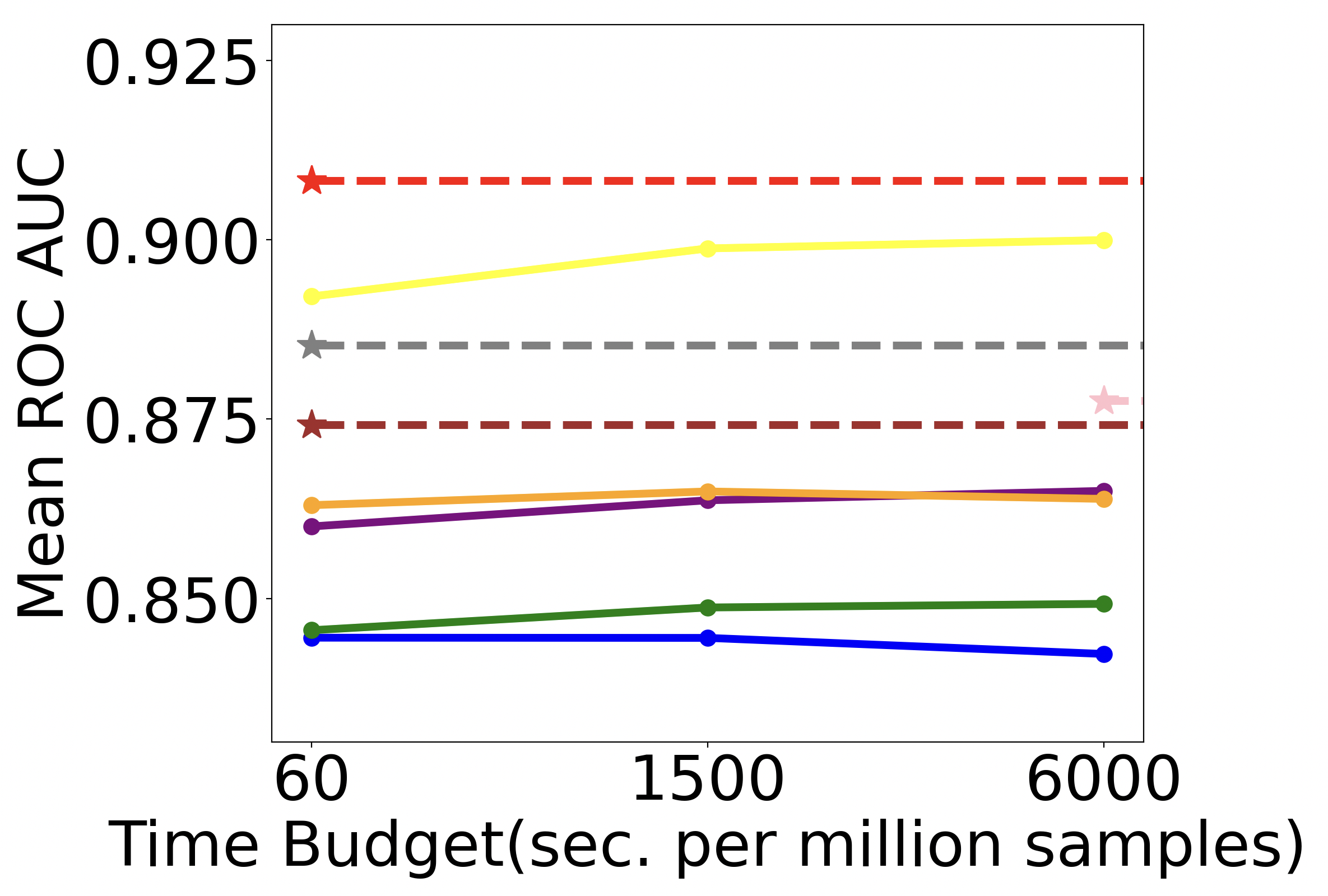
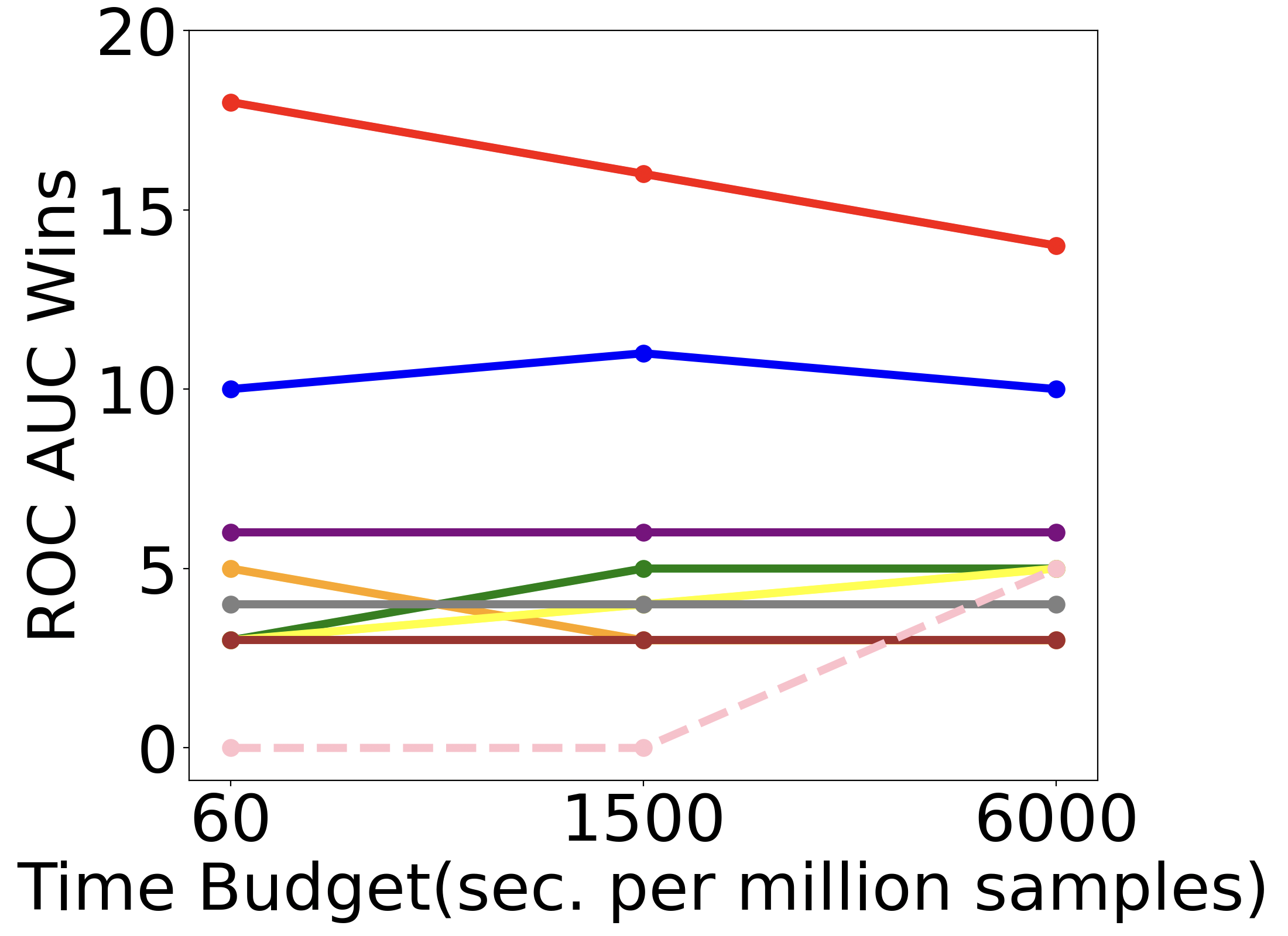
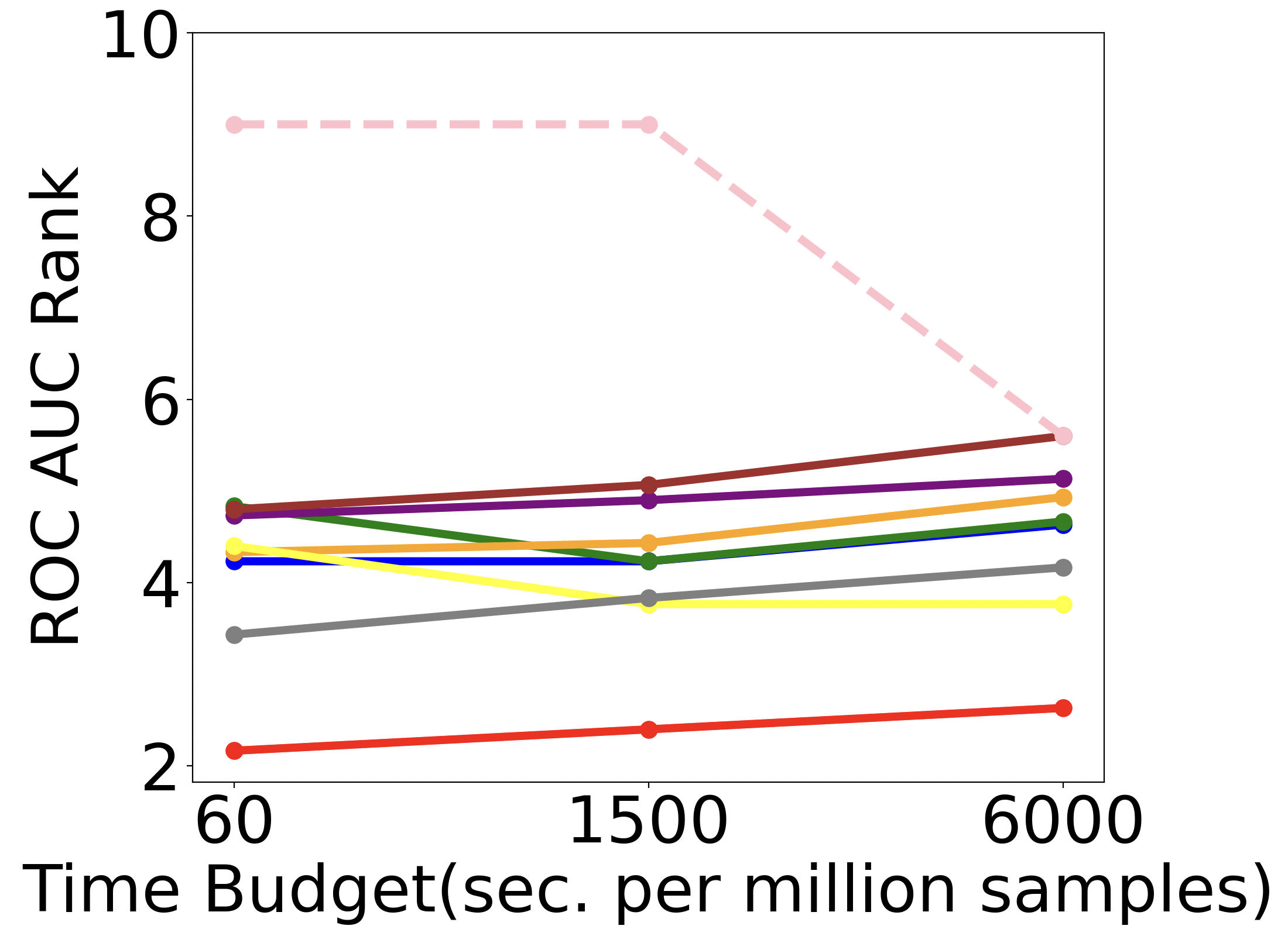
Figure 2: We show Mean AUC, Wins AUC and Mean Rank. as a function of the time allowed to train and tune methods, on large datasets with training number equals to 5,000 from OpenML benchmarks.

Efficiency. Next we show the performances of BoostPFN and baselines as the function of time limitation in Figure 2. All models use 5,000 training samples and details are shown in Supplemental Section E. The results show that BoostPFN can get best results when still maintaining efficiency, using much shorter time compared to GBDTs, deep learning methods and Autogluon, and a bit time longer than TabPFN and Bagging (While not shown in the figure, TabPFN costs about 12s and Bagging costs about 40s and BoostPFN costs about 60s per million samples). When more time is allowed, the results for baselines can be improved a bit.

7 Ablations

7.1 Emperical Validation of Assumption 4.1

We conduct the experiments based on TabPFN and on the dataset "analcatdata_dmft" that it performs not well [21]. We examine the performances of TabPFN when modifying the input training set.

Test Set. We first aim to determine the upper bound of TabPFN on the test set. The results are shown in Table 4. $D_{train}+D_{train}$ refers to the concatenation of two identical training sets. $D_{train}+D_{test}$ refers to the concatenation of the training set and the test set. $D_{train}+2D_{test}$ refers to the concatenation of the training set and two identical test sets. The results show that adding the test set as part of the input training set for TabPFN significantly improves its performance, with the upper bound being the results of using $D_{test}$ as the sole input training set. Duplicating the test set does not help TabPFN perform better on the test set, indicating that this is indeed the upper bound for this test set. This upper bound suggests some interference between test samples that could decrease performance, supporting Assumption 4.1. We further validate the assumption through experiments on a single test sample.

Table 4: Upper Bound of TabPFN on full test set.

Input Train set	$D_{train}+D_{train}$	$D_{train}+D_{test}$	$D_{train}+2D_{test}$
AUC OVO	0.5815	0.6812	0.7135
Input Train set	$D_{test}$	$D_{test}+D_{test}$
AUC OVO	0.7154	0.7154

Single Test Sample. Next, we demonstrate how the prediction for a single test sample depends on the input training samples. In Table 5, we show the probability of TabPFN predicting the correct label for just one test sample, $(x_{t1},y_{t1})$, from the same dataset.

First, we consider adding duplicates of the target sample to the training set. For this single sample, the input training set does not significantly aid the prediction, as the probability (0.192) is slightly higher than random guessing (0.167 for a 6-class classification task). Adding just one duplicate of this sample to the input training set improves the probability slightly. Adding two duplicates further increases the probability to 0.22. Subsequently, adding 10 duplicates increases the probability to 0.42, and adding 20 duplicates increases it to 0.75. Finally, adding 50 duplicates raises the probability to 0.94, and 100 duplicates to 0.98.

We then examine the results of replacing training samples with duplicates of the target sample. Similar to the trend observed when adding duplicates, replacing more training samples with the target sample also improves prediction accuracy (from 0.192 to 0.992 as the number of replacements increases from 0 to 100). Furthermore, with the same number of duplicates, replacing training samples performs better than simply adding them. This is reasonable because the training set with added duplicates contains more irrelevant samples than the training set where samples are replaced, further validating Assumption 4.1.

Table 5: Probability of TabPFN predicting the right class on single test sample. We show the number of adding or replacing with the probability.

# of Adding	0	1	2	10	20	50	100
Prob.	0.192	0.206	0.220	0.417	0.748	0.945	0.981
# of Replacing	0	1	2	10	20	50	100
Prob.	0.192	0.206	0.223	0.460	0.787	0.975	0.992

In a nutshell, TabPFN has performance upper bounds on the entire test set, even when duplicates of the test set are used as input. This may be because the prior is not well-suited for this dataset. However, for a specific sample, adding duplicates can increase the probability of predicting the correct class to as much as 98%, validating that adding the target sample improves performance, as stated in Assumption 4.1. Additionally, replacing training samples with the target sample also improves the probability, further supporting the notion that replacing irrelevant samples with the target sample enhances performance, as proposed in Assumption 4.1.

7.2 Sampling Weight Updates

In Section 4.2 we introduce three updating methods in the BoostPFN. Here we compare the results of those methods in Table 6. Exp., Hada. and Ada. stands for ExpHadamard, Hadamard and Adaboost updating respectively. The OVO AUC results are very close across different updating methods, showing the robustness towards them. However, in practice we encourage choosing the best one to get best results.

Table 6: Mean AUC OVO of three updating method in BoostPFN.

# of Training	Exp.	Hada.	Ada.
<5000	0.893	0.890	0.894
5000	0.900	0.898	0.905
50000	0.905	0.907	0.907
>50000	0.910	0.911	0.907

7.3 Emperical Convergence of BoostPFN

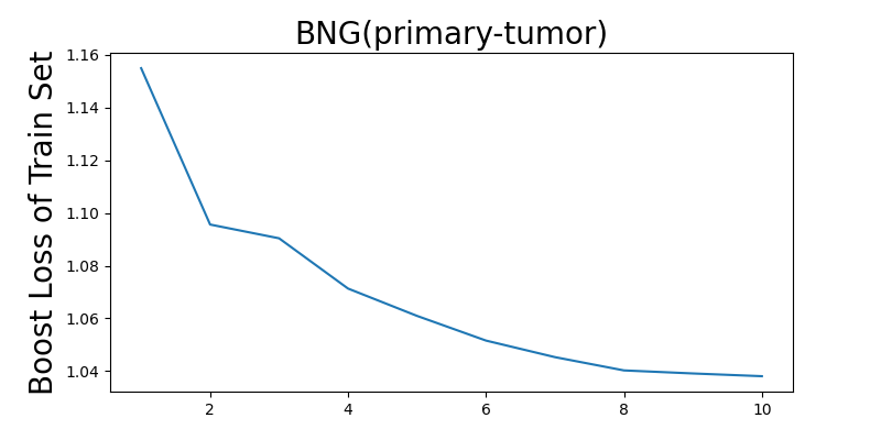
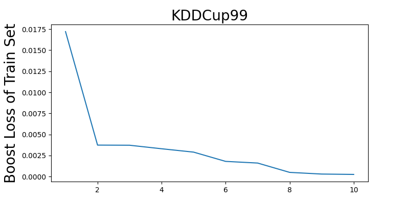
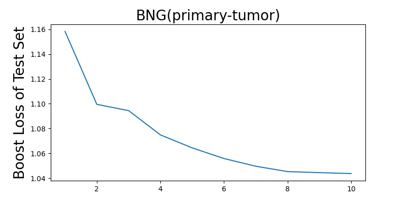
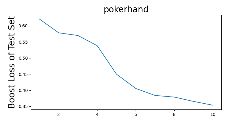
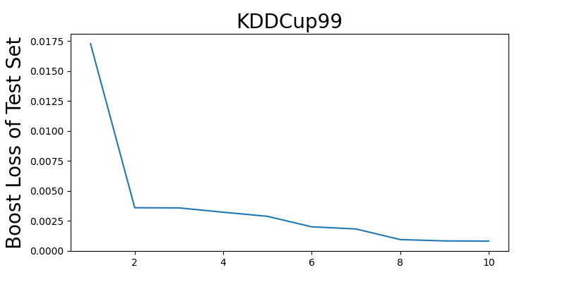
Figure 3: The first row shows boost loss on the training set of 3 datasets. The second row shows boost loss on the test set. The x-axis is the number of weak learners. From left to right, dataset order is BNG(primary-tumor), pokerhand, KDDCup99.

Although the fitting assumption of PFN is validated by experiments, we are curious about how the gradient boost actually works in large datasets. So we examine the boost loss on training set and test set and boost residual we used for gradient boost on training set. We use ExpHadamard Updating for the experiments. Full results of all datasets are showed in Appendix F, while we show the results of three datasets (BNG(primary-tumor), pokerhand, KDDCup99) in Figure 3, on which BoostPFN improves the best compared to TabPFN. We can find that when the number of weak learners increase, the boost loss on training set and test set decrease at the same time, showing the effectiveness of our method.

8 Related Works

Tabular Data Classification. Machine Learning methods and Deep Learning methods are two main types of method for tabular data classification. For Machine learning methods, variants of GBDTs [14] dominates this field mainly because of their fast training time and robustness [41]. LightGBM [27], CatBoost [36] and XGBoost [7] are three popular GBDTs applied in tabular data classification. Previous works have found that deep learning models are not better than the performance of GBDT or AutoML methods for small to medium-sized tabular data (< 10,000 samples; while matching GBDT performance on larger datasets) [5, 17, 42]. Furthermore, deep learning methods often use custom parameter tuning and preprocessing that makes the training on large datasets much more time-consuming, including FT-Transformer, SAINT, etc. [16, 43, 1, 25, 29]. There are also AutoML systems like AutoSklearn2 [13] and Autogluon [11]. AutoSklearn2 uses Bayesian Optimization and combines the evaluated models into a weighted ensemble and Autogluon combines a broad kind of models including neural networks and tree-based models into a stacked ensemble.

PFNs. PFNs are proposed by [33] on binary classification and small tabular datas of 100 samples. [21] further improve it to 10-class classification and medium-size (thousands of samples) tabular datas.  [34] analyze the statistical foundation of a single PFN and not an ensemble of PFNs. Larger datasets remain un-discovered in this field and our work extends the field of PFNs to larger datasets.

Ensemble for Transformers. Ensemble methods like AdaBoost [19] or Gradient Boosting [14, 15] are commonly applied on decision trees for better performances. Recently, Transformers are combined with AdaBoost in many fields. [23] integrate LLM into AdaBoost for natural language inference (NLI) tasks, by training an MLP projection of the final hidden state of a special token. [32] concentrates on condensing knowledge into an intermediary representation referred to as "summary." and applies AdaBoost for In-Context Learning for the prediction. However, their combination of summary sampling and AdaBoost are not theoretically validated. In this paper we propose a more generalized Gradient boosting method that is well validated theoretically and performs better in experiments.

9 Conclusion

In this paper, we have introduced BoostPFN, an innovative approach to scaling Prior-Fitted Networks (PFNs) for larger datasets, addressing the scalability challenges encountered by PFNs when applied to extensive data sets. Our method, through a meticulous investigation into the fitting assumptions of PFNs and the selection of input samples, presents a gradient boosting framework that significantly enhances the performance of PFNs, particularly on a large-scale. BoostPFN significantly extends the data size that PFNs can effectively process—up to 50 times the pre-training dataset size—while maintaining high performance compared to GBDTs, deep learning methods, and AutoML systems. We also provide a theoretical analysis that substantiates its convergence. BoostPFN offers a new perspective on handling large-scale tabular data classification tasks efficiently. In the future when PFNs are trained on larger datasets and perform better (for example, [22], which is published while our paper is under review), BoostPFN can still boost the predictions on much larger datasets with the new, better PFNs.

10 Acknowledgement

No acknowledgement to report at this time..

Checklist

1. For all models and algorithms presented, check if you include:

   1. A clear description of the mathematical setting, assumptions, algorithm, and/or model. [Yes]

   2. An analysis of the properties and complexity (time, space, sample size) of any algorithm. [Yes]

   3. (Optional) Anonymized source code, with specification of all dependencies, including external libraries. [Not Applicable]

2. For any theoretical claim, check if you include:

   1. Statements of the full set of assumptions of all theoretical results. [Yes]

   2. Complete proofs of all theoretical results. [Yes]

   3. Clear explanations of any assumptions. [Yes]

3. For all figures and tables that present empirical results, check if you include:

   1. The code, data, and instructions needed to reproduce the main experimental results (either in the supplemental material or as a URL). [Yes]

   2. All the training details (e.g., data splits, hyperparameters, how they were chosen). [Yes]

   3. A clear definition of the specific measure or statistics and error bars (e.g., with respect to the random seed after running experiments multiple times). [Yes]

   4. A description of the computing infrastructure used. (e.g., type of GPUs, internal cluster, or cloud provider). [Yes]

4. If you are using existing assets (e.g., code, data, models) or curating/releasing new assets, check if you include:

   1. Citations of the creator If your work uses existing assets. [Yes]

   2. The license information of the assets, if applicable. [Yes]

   3. New assets either in the supplemental material or as a URL, if applicable. [Yes]

   4. Information about consent from data providers/curators. [Yes]

   5. Discussion of sensible content if applicable, e.g., personally identifiable information or offensive content. [Not Applicable]

5. If you used crowdsourcing or conducted research with human subjects, check if you include:

   1. The full text of instructions given to participants and screenshots. [Not Applicable]

   2. Descriptions of potential participant risks, with links to Institutional Review Board (IRB) approvals if applicable. [Not Applicable]

   3. The estimated hourly wage paid to participants and the total amount spent on participant compensation. [Not Applicable]

Appendix A Additional Theoretical Analysis

A.1 A simplified Scenerio for Dataset Optimization

We consider a simplified scenario in which we need to update the sampling weights from a uniform distribution.

Lemma A.1.

Given a training set $D$, $N=|D|$ is the number of training samples. We do the non-replacement sampling in $D$ with the sampling size $z$ and uniform sampling weights $w_{1}=(p_{1}^{w_{1}},p_{2}^{w_{1}},...p_{N}^{w_{1}})$, where each $p_{a}^{w_{1}}=p_{0}=\frac{1}{N}$ for $a\in(1,2,...,N)$. Then with a new set of sampling weights $w_{2}$ where $p_{i}^{w_{2}}=kp_{i}^{w_{1}}$ and $p_{j}^{w_{2}}=\lambda p_{j}^{w_{1}}$ for all $j\in(1,2,...,N)$ and $j\neq i$, where $k<N$ and $\lambda=\frac{1-kp_{0}}{1-p_{0}}$ to maintain normalization, given Assumption 4.1 and for $k>(N-z)(1-\lambda_{B})+1$, the expectation of predicting the right label on target $i$ is larger than with $w_{1}$ :

$$\mathbb{E}[q_{(\theta,w_{2})}(y_{i}|x_{i},D)]>\mathbb{E}[q_{(\theta,w_{1})}(y_{i}|x_{i},D)],$$ (13)

where $0<\lambda_{B}<1$ and is defined in Eq. 23.

We put the proof below.

Proof.

First we write the expectation in

$$\mathbb{E}[q_{(\theta,w)}(y_{i}|x_{i},D)]=\sum_{D_{w}^{z}\in\mathcal{D}^{z}}p(D_{w}^{z})q_{\theta}(y_{i}|x_{i},D_{w}^{z}),$$ (14)

where $\mathcal{D}^{z}$ is the space of all possibilities of non-replacement sampling with size $z$.

Now we consider the situation that $D^{z}=D_{0}\cup(x_{i},y_{i})$, then there are $(N-z)$ situations that $\bar{D}^{z}=D_{0}\cup(x_{j},y_{j})$ where $(x_{j},y_{j})\notin D^{z}$. So the expectation can be written as

$$\mathbb{E}[q_{(\theta,w)}(y_{i}|x_{i},D)]=\sum_{D^{z}}\Big{[}p(D^{z};w)q_{\theta}(y_{i}|x_{i},D^{z})+\sum_{\bar{D}^{z}}p(\bar{D}^{z};w)q_{\theta}(y_{i}|x_{i},\bar{D}^{z})\Big{]}.$$ (15)

Let $A(w)=p(D^{z};w)q_{\theta}(y_{i}|x_{i},D^{z})$ and $B(w)=\sum_{\bar{D}^{z}}p(\bar{D}_{w}^{z};w)q_{\theta}(y_{i}|x_{i},\bar{D}^{z})$. To prove Eq. 13, we need to show that $A(w_{2})+B(w_{2})>A(w_{1})+B(w_{1})$.

In the non-replacement sampling, if we use $p_{a}$ to denote the $a$th sample’s weight, $A(w_{1})$ can be written as

$$A(w_{1}) =\frac{z!\cdot\prod_{a=1}^{z}p_{a}}{\prod_{a=1}^{z}(1-\sum_{b=1}^{a-1}p_{b})}q_{\theta}(y_{i}|x_{i},D^{z}),$$ (16)

$$=\frac{z!}{\binom{N}{z}}q_{\theta}(y_{i}|x_{i},D^{z}),\text{ remembering each weight is $p_{0}=\frac{1}{N}$ for $w_{1}$}.$$

Then we compute $A(w_{2})$, remembering that in $w_{2}$, $p_{i}^{w_{2}}=kp_{0}$ and for $a\neq i$, $p_{a}^{w_{2}}=\lambda p_{0}=\frac{1-kp_{0}}{1-p_{0}}p_{0}$,

$$A(w_{2}) =\frac{z!\cdot p_{i}\cdot\prod_{a=1}^{z-1}p_{a}^{w_{2}}}{\prod_{a=1}^{z}(1-\sum_{b=1}^{a-1}p_{b}^{w_{2}})}q_{\theta}(y_{i}|x_{i},D^{z}),$$ (17)

$$=\frac{z!\cdot\left(k\cdot\frac{1}{N}\right)\cdot\left(\lambda\cdot\frac{1}{N}\right)^{z-1}}{\frac{N\cdot(N-k)\cdot(N-k-\lambda)\cdots(N-k-(z-2)\lambda)}{N^{z}}}q_{\theta}(y_{i}|x_{i},D^{z})$$

$$=k\cdot\lambda^{z-1}\cdot\frac{z!\cdot N^{z}}{N\cdot(N-k)\cdot(N-k-\lambda)\cdots(N-k-(z-2)\lambda)}q_{\theta}(y_{i}|x_{i},D^{z})$$

So

$$\frac{A(w_{2})}{A(w_{1})} =\frac{k\cdot\lambda^{z-1}\cdot\frac{z!\cdot N^{z}}{N\cdot(N-k)\cdot(N-k-\lambda)\cdots(N-k-(z-2)\lambda)}}{\frac{z!}{\binom{N}{z}}}$$ (18)

$$=k\cdot\lambda^{z-1}\cdot N^{z}\cdot\frac{\binom{N}{z}}{N\cdot(N-k)\cdot(N-k-\lambda)\cdots(N-k-(z-2)\lambda)}$$

$$=k\cdot\lambda^{z-1}\cdot\frac{N\cdot(N-1)\cdot(N-2)\cdots(N-(z-1))}{N\cdot(N-k)\cdot(N-k-\lambda)\cdots(N-k-(z-2)\lambda)}$$

Note that

$$\lambda =\frac{1-kp_{0}}{1-p_{0}}=\frac{1-k\frac{1}{N}}{1-\frac{1}{N}}=\frac{N-k}{N-1},$$ (19)

so

$$\frac{N-1}{N-k}=\frac{N-2}{N-k-\lambda}=\cdots=\frac{N-(z-1)}{N-k-(z-2)\lambda}=\frac{1}{\lambda}.$$ (20)

Then

$$\frac{A(w_{2})}{A(w_{1})}=k\cdot\lambda^{z-1}\cdot\lambda^{1-z}=k.$$ (21)

Using the same process we can compute that

$$\frac{B(w_{2})}{B(w_{1})} =\lambda^{z}\frac{\prod_{a=1}^{z}(1-\sum_{b=1}^{a-1}p_{0})}{\prod_{a=1}^{z}(1-\sum_{b=1}^{a-1}\lambda p_{0})}.$$ (22)

We then define

$$\lambda_{B}\triangleq\lambda^{z}\frac{\prod_{a=1}^{z}(1-\sum_{b=1}^{a-1}p_{0})}{\prod_{a=1}^{z}(1-\sum_{b=1}^{a-1}\lambda p_{0})}.$$ (23)

With $0<\lambda<1$ we know $0<\lambda_{B}<1$. So

$$A(w_{2})+B(w_{2})>A(w_{1})+B(w_{1}) \Longleftrightarrow kA(w_{1})+\lambda_{B}B(w_{1})>A(w_{1})+B(w_{1})$$ (24)

$$\Longleftrightarrow(k-1)A(w_{1})>(1-\lambda_{B})B(w_{1})$$

$$\Longleftrightarrow\frac{A(w_{1})}{B(w_{1})}>\frac{1-\lambda_{B}}{k-1}.$$

Remembering the definition of $A(w_{1})$ and $B(w_{1})$, we know that

$$\frac{A(w_{1})}{B(w_{1})}=\frac{q_{\theta}(y_{i}|x_{i},D^{z})}{(N-z)q_{\theta}(y_{i}|x_{i},\bar{D}^{z})}>\frac{1}{(N-z)},\text{~~~ Given Assumption \ref{prop:fittingassumption}.}$$ (25)

So Eq. 24 holds if

$$\frac{1}{(N-z)}>\frac{1-\lambda_{B}}{k-1}.$$ (26)

This is true because $k>(N-z)(1-\lambda_{B})+1$ is one of our condition. Then we complete the proof of Lemma A.1. ∎

A.2 Proof for Theorem 5.1

We begin the proof by the first proving that BoostPFN is a kind of Randomized Gradient Boosting Machine.

Remark A.2.

BoostPFN showed in Algorithm 1 is a kind of Randomized Gradient Boosting Machine.

Proof.

Randomized Gradient Boosting Machine can be written as

 Initialization. Initialize with $f^{0}(x)=0$.

For $m=0,\ldots,M-1$ do:

   (1) Compute pseudo-residual $r^{m}=-\left[\frac{\partial\ell(y_{i},f^{m}(x_{i}))}{\partial f^{m}(x_{i})}\right]_{i=1,\ldots,n}.$

   (2) Pick a random subset $J$ of weak-learners by some rule (i.e., one of Type 0 - Type 3)

   (3) Find the best weak-learner in $J$: $j_{m}=\text{argmin}_{j\in J}\min_{\sigma}\sum_{i=1}^{n}(r^{m}_{i}-\sigma b(x_{i};\tau_{j}))^{2}$.

   (4) Choose the step-size $\rho_{m}$ by one of the following rules:

      $\bullet$ line-search: $\rho_{m}=\text{argmin}_{\rho}\sum_{i=1}^{n}\ell(y_{i},f^{m}(x_{i})+\rho b(x_{i};\tau_{j_{m}}))$;

      $\bullet$ constant step-size: $\rho_{m}=\rho\left(\sum_{i=1}^{n}r_{i}^{m}b(x_{i};\tau_{j_{m}})\right)$, where $\rho$ is a constant specified a priori.

   (5) Update the model $f^{m+1}(x)=f^{m}(x)+\rho_{m}b(x;\tau_{j_{m}})$.

 Output. $f^{M}(x)$.

Algorithm 2 Randomized Gradient Boosting Machine (RGBM)

from [31]. $b(x_{i};\tau_{j_{m}})$ is the weak learner in round $m$. Type 0 to Type 3 are as follows :

• [Type 0]: (Full Deterministic Selection) We choose $J$ as the whole set of weak-learners. This is a deterministic selection rule.

• [Type 1]: (Random Selection) We choose uniformly at random $t$ weak-learners from all possible weak-learners without replacement—the collection is denoted by $J$.

• [Type 2]: (Random Single Group Selection) Given a non-overlapping partition of the weak-learners, we pick one group uniformly at random and denote the collection of weak-learners in that group by $J$.

• [Type 3]: (Random Multiple Group Selection) Given a non-overlapping partition of the weak-learners, we pick $t$ groups uniformly at random and let the collection of weak-learners across these groups be $J$.

When we compare RGBM with BoostPFN, it’s clear that if we choose line-search in step (4) of RGBM, the difference is in step (2) and (3). Here we show that the weights updating is actually picking random subset of weak learner.

We write the subset of TabPFN as $J=\{q_{\theta}(\cdot|x,D_{w}^{z})|D_{w}\text{ generated by }w\}$. In BoostPFN algorithm, we sample a weak learner from the subset instead of choosing the best one. So we need to modify the algorithm a bit here. We introduce the union of subset with different sampling weights $J_{U}=\bigcup_{i=0,1,2}J_{i}=\{q_{\theta}(\cdot|x,D_{w_{i}}^{z})|D_{w_{i}}^{z}\text{ generated by }w_{i}\}$ where $w_{0}$ is uniform sampling weights, $w_{1}$ is the sampling weights for this round of boost, $w_{2}$ is the sampling weights for last round. And we choose the best weak learner in this subset. The subset is picked via Type 3. Thus BoostPFN with this modification is the same as RGBM. ∎

Then the Theorem 4.2 in [31] that the RGBM in Algorithm 2 if $\ell$ is a $\sigma$-smooth function and has a bounded level set will converge with the rate of $O(\frac{\sigma}{M})$ will lead straightforwardly to the proof of Eq. 12.

Appendix B Experimental Implementation and Hyperparameters

We do all experiments on a platform with 48 CPU cores and RTX 3090. For ensemble models on small datasets, we use sampling size 0.5 of the training set if training set contains less than 1000 samples. The hyperparameter spaces for LightGBM, CatBoost and XGBoost follow [21] and are shown in Table 7.

Table 7: Hyperparameter spaces for baselines.

baseline	name	type	log	range
LightGBM	num_leaves	int	[5, 50]	yes
	max_depth	int	[3, 20]	yes
	learning_rate	float	[$e^{-3}$, 1]	-
	n_estimators	int	50, 2000	-
	min_child_weight	float	[$e^{-5}$, $e^{4}$]	yes
	reg_alpha	float	[0, 1e-1, 1, 2, 5, 7, 10, 50, 100]	yes
	reg_lambda	float	[0, 1e-1, 1, 5, 10, 20, 50, 100]	yes
	subsample	float	[0.2, 0.8]	-
CatBoost	learning_rate	float	[$e^{-5}$, 1]	yes
	random_strength	int	[1, 20]	-
	l2_leaf_reg	float	[1, 10]	yes
	bagging_temperature	float	[0, 1.0]	yes
	leaf_estimation_iterations	int	[1, 20]	-
	iterations	int	[100, 4000]	-
XGBoost	learning_rate	float	[$e^{-7}$, 1]	yes
	max_depth	int	[1, 10]	-
	subsample	float	[0.2, 1]	-
	colsample_bytree	float	[0.2, 1]	-
	colsample_bylevel	float	[0.2, 1]	-
	min_child_weight	float	[$e^{-16}$, $e^{5}$]	yes
	alpha	float	[$e^{-16}$, $e^{2}$]	yes
	lambda	float	[$e^{-16}$, $e^{2}$]	yes
	gamma	float	[$e^{-16}$, $e^{2}$]	yes
	n_estimators	int	[100, 4000]	-

For AutoGluon we use "best quality". For FT-Transformer we tuning learning rate in [5e-5,1e-4,5e-4,1e-3], batch size in [128, 256, 512, 1024]. For SAINT we use default setting because it costs too much time to tuning.

For tuning methods, time limitation is 6000 seconds per million samples.

Appendix C Datasets Statistics

We show the dataset statistics for small datasets in Table 8, cited from [21]. Large datasets statistics are shown in Table 9.

Table 8: Small datasets used for the evaluation. All 30 datasets are at most $2\,000$ samples, $100$ features and $10$ classes.

Name	#Feat.	#Cat.	#Inst.	#Class.	#NaNs	Minor. Class Size	OpenML ID
balance-scale	5	1	625	3	0	49	11
mfeat-fourier	77	1	2000	10	0	200	14
breast-w	10	1	699	2	16	241	15
mfeat-karhunen	65	1	2000	10	0	200	16
mfeat-morphological	7	1	2000	10	0	200	18
mfeat-zernike	48	1	2000	10	0	200	22
cmc	10	8	1473	3	0	333	23
credit-approval	16	10	690	2	67	307	29
credit-g	21	14	1000	2	0	300	31
diabetes	9	1	768	2	0	268	37
tic-tac-toe	10	10	958	2	0	332	50
vehicle	19	1	846	4	0	199	54
eucalyptus	20	6	736	5	448	105	188
analcatdata_auth…	71	1	841	4	0	55	458
analcatdata_dmft	5	5	797	6	0	123	469
pc4	38	1	1458	2	0	178	1049
pc3	38	1	1563	2	0	160	1050
kc2	22	1	522	2	0	107	1063
pc1	22	1	1109	2	0	77	1068
banknote-authenti…	5	1	1372	2	0	610	1462
blood-transfusion-…	5	1	748	2	0	178	1464
ilpd	11	2	583	2	0	167	1480
qsar-biodeg	42	1	1055	2	0	356	1494
wdbc	31	1	569	2	0	212	1510
cylinder-bands	40	22	540	2	999	228	6332
dresses-sales	13	12	500	2	835	210	23381
MiceProtein	82	5	1080	8	1396	105	40966
car	7	7	1728	4	0	65	40975
steel-plates-fault	28	1	1941	7	0	55	40982
climate-model-simu…	21	1	540	2	0	46	40994

Table 9: Large datasets used for the evaluation. All 30 datasets are at most 10 million samples, 100 features and 144 classes.

Name	#Feat.	#Cat.	#Inst.	#Class.	#NaNs	Minor. Class Size	OpenML ID
BNG(page-blocks,nominal,295245)	11	11	295245	5	0	1558	125
BNG(glass,nominal,137781)	10	10	137781	7	0	307	133
BNG(heart-c,nominal,1000000)	14	14	1000000	5	0	1618	136
BNG(heart-h,nominal,1000000)	14	14	1000000	5	0	1659	138
BNG(waveform-5000,nominal,1000000)	41	41	1000000	3	0	330548	147
pokerhand	11	6	829201	10	0	2	155
RandomRBF_0_0	11	1	1000000	5	0	92713	156
RandomRBF_10_1E-3	11	1	1000000	5	0	92713	157
RandomRBF_10_1E-4	11	1	1000000	5	0	92713	158
SEA(50)	4	1	1000000	2	0	385658	161
SEA(50000)	4	1	1000000	2	0	385668	162
BNG(heart-c)	14	8	1000000	5	0	1609	266
BNG(primary-tumor)	18	18	1000000	22	0	1417	1177
BNG(solar-flare)	13	13	1000000	3	0	1393	1179
Stagger1	4	4	1000000	2	0	111609	1236
Stagger2	4	4	1000000	2	0	444057	1237
Stagger3	4	4	1000000	2	0	333571	1238
AirlinesCodrnaAdult	30	17	1076790	2	7275	473652	1240
skin-segmentation	4	1	245057	2	0	50859	1502
creditcard	31	1	284807	2	0	492	1597
BNG(spambase)	58	58	1000000	2	0	394052	40515
BNG(anneal)	39	33	1000000	6	0	555	40520
fars	30	16	100968	8	0	9	40672
seattlecrime6	8	6	523590	144	6916	1	41960
porto-seguro	38	26	595212	2	846458	21694	42206
CreditCardFraudDetection	31	1	284807	2	0	492	42397
KDDCup99	42	10	4898431	23	0	2	42746
bates_classif_20	21	1	5100000	2	0	2549577	45654
colon	63	1	5100000	2	0	2549437	45665
breast	78	1	5100000	2	0	2549502	45669

Appendix D Full Experiment Results

We show the per dataset results on small datasets with a 1 hour time limit in Table 10. The large datasets results with different number of training samples are showed in Table 11,12 and 13 .

Table 10: Per dataset results on small datasets lower than 5000 training samples.

	LightGBM	CatBoost	XGBoost	AutoGluon	FT-Trans.	SAINT	TabPFN	Bagging	BoostPFN
balance-scale	0.9938	0.9245	0.9939	0.9919	0.9935	0.86366	0.9973	0.9985	0.9996
mfeat-fourier	0.9786	0.9816	0.9803	0.9843	0.9782	0.978938	0.9811	0.9761	0.9769
breast-w	0.991	0.9931	0.9896	0.9933	0.9846	0.987477	0.9934	0.9922	0.9921
mfeat-karhunen	0.9979	0.9986	0.9983	0.9987	0.9961	0.998036	0.9978	0.9981	0.999
mfeat-morphologica..	0.9601	0.9629	0.9612	0.9698	0.9665	0.95501	0.9669	0.9669	0.9664
mfeat-zernike	0.9716	0.9759	0.9735	0.9908	0.9808	0.973376	0.9823	0.9834	0.9833
cmc	0.7288	0.7256	0.7299	0.7331	0.7073	0.699643	0.7276	0.7173	0.7205
credit-approval	0.9415	0.9389	0.9422	0.9415	0.9175	0.933137	0.9322	0.9424	0.9427
credit-g	0.7684	0.7852	0.7853	0.7941	0.7644	0.602838	0.7894	0.7916	0.7918
diabetes	0.8247	0.8383	0.8378	0.8391	0.8475	0.650567	0.841	0.8251	0.8239
tic-tac-toe	0.9988	0.9992	1	1	0.9935	0.562474	0.9759	0.9437	0.9767
vehicle	0.9232	0.9302	0.9282	0.9416	0.9357	0.923496	0.9589	0.9563	0.9597
eucalyptus	0.8931	0.8979	0.9004	0.9204	0.8961	0.851701	0.9245	0.9196	0.9227
analcatdata_author..	0.9999	0.9999	0.9997	0.9993	0.9972	0.999019	1	1	1
analcatdata_dmft	0.5461	0.5589	0.5743	0.5657	0.5489	0.551028	0.579	0.5811	0.5806
pc4	0.9301	0.9413	0.9291	0.9428	0.9254	0.914273	0.9383	0.9207	0.9247
pc3	0.8178	0.8247	0.8288	0.8282	0.7911	0.808226	0.8373	0.8513	0.8518
kc2	0.8141	0.8323	0.8227	0.8242	0.8059	0.846287	0.8346	0.8705	0.8698
pc1	0.8321	0.86	0.8489	0.8578	0.7207	0.805705	0.8761	0.8936	0.8876
banknote-authentic..	1	1	1	1	0.9927	0.992147	1	1	1
blood-transfusion-..	0.7144	0.7403	0.7312	0.7364	0.7803	0.928475	0.7549	0.7747	0.7687
ilpd	0.6917	0.7279	0.7171	0.723	0.7044	0.619734	0.7379	0.7523	0.7527
qsar-biodeg	0.9126	0.9217	0.9191	0.9276	0.9202	0.999062	0.9336	0.9282	0.9288
wdbc	0.9904	0.9931	0.9904	0.9956	0.986	0.709422	0.9964	0.9985	0.9988
cylinder-bands	0.8556	0.8757	0.8782	0.8878	0.8038	0.790092	0.8336	0.7802	0.7969
dresses-sales	0.5593	0.5696	0.5823	0.5507	0.5056	0.578095	0.5376	0.5559	0.5532
MiceProtein	0.9997	0.9999	0.9998	1	0.9992	0.999702	0.9999	0.9998	1
car	0.9925	0.9955	0.9948	0.997	0.9849	0.953275	0.995	0.9902	0.9965
steel-plates-fault..	0.9626	0.9655	0.9656	0.9666	0.9532	0.59391	0.9655	0.9595	0.9587
climate-model-simu..	0.9286	0.9344	0.9255	0.9391	0.8719	0.666173	0.9415	0.926	0.9298
Mean AUC OVO	0.884$\pm$.012	0.89$\pm$.011	0.891$\pm$.011	0.895$\pm$.011	0.875$\pm$.010	0.824$\pm$.011	0.894$\pm$.010	0.893$\pm$.010	0.895$\pm$.009

Table 11: Per dataset results on large datasets with 5,000 training samples.

	LightGBM	CatBoost	XGBoost	AutoGluon	FT-Trans.	SAINT	TabPFN	Bagging	BoostPFN
BNG(page-blocks,nominal,295245)	0.8401	0.8385	0.8296	0.7812	0.8478	0.7531	0.81	0.7851	0.8473
BNG(glass,nominal,137781)	0.9011	0.8979	0.8994	0.8322	0.9013	0.9007	0.8907	0.8395	0.8824
BNG(heart-c,nominal,1000000)	0.7664	0.7779	0.7825	0.6283	0.8019	0.7876	0.7856	0.7754	0.8072
BNG(heart-h,nominal,1000000)	0.829	0.7803	0.793	0.6898	0.8156	0.7867	0.8001	0.786	0.8188
BNG(waveform-5000,nominal,1000000)	0.9569	0.9567	0.9572	0.9579	0.9541	0.9568	0.9536	0.9535	0.9536
pokerhand	0.636	0.6512	0.6205	0.6134	0.9395	0.9011	0.6894	0.7725	0.9632
RandomRBF_0_0	0.9878	0.9884	0.9886	0.9927	0.9872	0.9898	0.9915	0.9902	0.9918
RandomRBF_10_1E-3	0.9554	0.9591	0.9592	0.9671	0.9554	0.9598	0.9623	0.9607	0.9629
RandomRBF_10_1E-4	0.9635	0.9667	0.9659	0.9758	0.9627	0.9654	0.9727	0.9675	0.9701
SEA(50)	0.8728	0.8768	0.8761	0.8781	0.8765	0.8688	0.8776	0.8777	0.8773
SEA(50000)	0.8736	0.8754	0.8755	0.8781	0.8771	0.8803	0.8769	0.8774	0.8765
BNG(heart-c)	0.7768	0.7712	0.7676	0.727	0.7564	0.7594	0.7618	0.7514	0.7598
BNG(primary-tumor)	0.9009	0.8915	0.8977	0.8558	0.891	0.8473	0.8347	0.8443	0.8908
BNG(solar-flare)	0.8783	0.8673	0.8698	0.8527	0.8628	0.8303	0.8448	0.8323	0.8867
Stagger1	1	1	1	1	1	1	1	1	1
Stagger2	1	1	1	1	1	1	1	1	1
Stagger3	1	1	1	1	1	1	1	1	1
AirlinesCodrnaAdult	0.8738	0.8761	0.8756	0.8822	0.8753	0.8525	0.8702	0.8679	0.8708
skin-segmentation	0.9997	0.9998	0.9998	1	0.9999	0.9985	0.9999	0.9995	1
creditcard	0.947	0.9621	0.9616	0.961	0.9624	0.9435	0.9763	0.9601	0.9844
BNG(spambase)	0.6452	0.6615	0.6659	0.6632	0.6618	0.3719	0.6596	0.6532	0.6588
BNG(anneal)	0.9618	0.9622	0.9627	0.8851	0.9643	0.9491	0.952	0.9351	0.9624
fars	0.5021	0.4896	0.4972	0.4969	0.8509	0.8552	0.8751	0.8059	0.8774
seattlecrime6	0.988	0.9882	0.5022	0.8889	0.9902	0.9452	0.9879	0.9	0.9926
porto-seguro	0.5742	0.5993	0.5983	0.5955	0.5941	0.5632	0.5919	0.5921	0.6086
CreditCardFraudDetection	0.9732	0.9611	0.9556	0.9466	0.9706	0.9355	0.9699	0.9698	0.9828
KDDCup99	0.5196	0.5248	0.5181	0.5248	0.835	0.8876	0.7609	0.674	0.9535
bates_classif_20	0.8701	0.8689	0.8727	0.8737	0.8754	0.8684	0.8774	0.8771	0.8761
colon	0.9939	0.9936	0.9949	0.9967	0.9969	0.9976	0.996	0.9916	0.9972
breast	0.9626	0.9613	0.975	0.9903	0.9925	0.9715	0.9895	0.9862	0.9934
Mean AUC OVO	0.865$\pm$.001	0.865$\pm$.001	0.849$\pm$.001	0.844$\pm$.001	0.900$\pm$.002	0.878$\pm$.002	0.885$\pm$.001	0.874$\pm$.001	0.908$\pm$.001

Table 12: Per dataset results on large datasets with 50,000 training samples.

	LightGBM	CatBoost	XGBoost	AutoGluon	FT-Trans.	SAINT	TabPFN	Bagging	BoostPFN
BNG(page-blocks,nominal,295245)	0.854	0.8575	0.8518	0.8415	0.8575	0.8445	OOM	0.8209	0.8427
BNG(glass,nominal,137781)	0.9151	0.9091	0.9155	0.9129	0.916	0.9126	OOM	0.8936	0.8941
BNG(heart-c,nominal,1000000)	0.8125	0.7999	0.8066	0.8102	0.811	0.808	OOM	0.7767	0.802
BNG(heart-h,nominal,1000000)	0.8198	0.8042	0.813	0.8137	0.8095	0.8161	OOM	0.7872	0.8193
BNG(waveform-5000,nominal,1000000)	0.9631	0.9619	0.9636	0.9583	0.9616	0.9626	OOM	0.9548	0.9536
pokerhand	0.4945	0.5275	0.4923	0.4981	0.9625	0.8915	OOM	0.7813	0.9752
RandomRBF_0_0	0.9929	0.9902	0.9916	0.993	0.9935	0.994	OOM	0.9909	0.9924
RandomRBF_10_1E-3	0.9649	0.9627	0.9673	0.9685	0.9701	0.9678	OOM	0.9634	0.964
RandomRBF_10_1E-4	0.9767	0.9718	0.9774	0.9826	0.9827	0.9806	OOM	0.9697	0.9745
SEA(50)	0.8817	0.8811	0.8808	0.89	0.8775	0.8731	OOM	0.8783	0.8767
SEA(50000)	0.8806	0.8805	0.8805	0.8892	0.877	0.8729	OOM	0.8779	0.8767
BNG(heart-c)	0.7977	0.77	0.7828	0.7911	0.7924	0.7641	OOM	0.7633	0.7684
BNG(primary-tumor)	0.9104	0.9163	0.9134	0.8695	0.9138	0.9072	OOM	0.8548	0.8901
BNG(solar-flare)	0.9121	0.9001	0.9061	0.8808	0.9018	0.8796	OOM	0.8416	0.8772
Stagger1	1	1	1	1	1	1	OOM	1	1
Stagger2	1	1	1	1	1	1	OOM	1	1
Stagger3	1	1	1	1	1	1	OOM	1	1
AirlinesCodrnaAdult	0.8921	0.8932	0.5006	0.8967	0.8915	0.8937	OOM	0.8709	0.8751
skin-segmentation	0.9999	0.9999	1	1	0.9999	0.9998	OOM	0.9999	1
creditcard	0.9756	0.974	0.9721	0.9781	0.9719	0.9492	OOM	0.9683	0.9833
BNG(spambase)	0.6688	0.6695	0.669	0.6693	0.6689	0.661	OOM	0.6614	0.6577
BNG(anneal)	0.98	0.9818	0.9778	0.9875	0.9884	0.9856	OOM	0.9372	0.9712
fars	0.8866	0.8867	0.9086	0.8566	0.8937	0.9003	OOM	0.859	0.8768
seattlecrime6	0.9898	0.5105	0.5042	0.5041	0.9891	0.9637	OOM	0.9906	0.9913
porto-seguro	0.6084	0.5675	0.6034	0.6257	0.6192	0.6153	OOM	0.6141	0.6136
CreditCardFraudDetection	0.9766	0.9757	0.9742	0.9779	0.9639	0.9656	OOM	0.9703	0.9824
KDDCup99	0.4863	0.4869	0.5352	0.4974	0.8298	0.9276	OOM	0.7649	0.9606
bates_classif_20	0.8746	0.8744	0.874	0.8782	0.8779	0.8905	OOM	0.8784	0.8775
colon	0.9965	0.9965	0.9962	0.9973	0.9976	1	OOM	0.9915	0.9974
breast	0.9826	0.9749	0.9844	0.9776	0.9942	0.9904	OOM	0.9898	0.9942
Mean AUC OVO	0.883$\pm$.001	0.864$\pm$.001	0.855$\pm$.001	0.865$\pm$.001	0.910$\pm$.001	0.907$\pm$.001	OOM	0.8888$\pm$.001	0.910$\pm$.001

Table 13: Per dataset results on large datasets with full training samples.

	LightGBM	CatBoost	XGBoost	AutoGluon	FT-Trans.	SAINT	TabPFN	Bagging	BoostPFN
BNG(page-blocks,nominal,295245)	0.8587	0.8602	0.8598	0.8456	0.8619	0.8472	OOM	0.8149	0.8471
BNG(glass,nominal,137781)	0.9154	0.9148	0.9092	0.9129	0.918	0.9152	OOM	0.8936	0.9
BNG(heart-c,nominal,1000000)	0.8137	0.8148	0.8105	0.8104	0.8196	0.817	OOM	0.777	0.8052
BNG(heart-h,nominal,1000000)	0.8205	0.8221	0.8216	0.822	0.8246	0.8194	OOM	0.7877	0.8138
BNG(waveform-5000,nominal,1000000)	0.9663	0.9667	0.9659	0.9649	0.9654	0.9643	OOM	0.9551	0.9561
pokerhand	0.8174	0.8751	0.8782	0.8968	0.9721	0.9555	OOM	0.8096	0.968
RandomRBF_0_0	0.9948	0.9934	0.9925	0.9951	0.9959	0.9959	OOM	0.9909	0.9929
RandomRBF_10_1E-3	0.9761	0.9706	0.9678	0.981	0.9814	0.9811	OOM	0.9636	0.9658
RandomRBF_10_1E-4	0.9866	0.9804	0.9771	0.9884	0.99	0.9904	OOM	0.97	0.975
SEA(50)	0.9083	0.901	0.9162	0.9824	0.8767	0.8779	OOM	0.8782	0.8784
SEA(50000)	0.9047	0.899	0.892	0.9824	0.8782	0.8777	OOM	0.878	0.878
BNG(heart-c)	0.8013	0.7987	0.7935	0.7955	0.7998	0.7995	OOM	0.7649	0.779
BNG(primary-tumor)	0.9188	0.9203	0.9181	0.9174	0.918	0.9139	OOM	0.8557	0.902
BNG(solar-flare)	0.9262	0.9235	0.9207	0.9046	0.9346	0.928	OOM	0.8454	0.8946
Stagger1	1	1	1	1	1	1	OOM	1	1
Stagger2	1	1	1	1	1	1	OOM	1	1
Stagger3	1	1	1	1	1	1	OOM	1	1
AirlinesCodrnaAdult	0.9102	0.9035	0.9024	0.9134	0.9038	0.9029	OOM	0.8713	0.8822
skin-segmentation	1	1	1	1	1	0.9997	OOM	0.9999	1
creditcard	0.9799	0.9802	0.9802	0.9834	0.9778	0.9777	OOM	0.9712	0.982
BNG(spambase)	0.6723	0.6722	0.672	0.6717	0.6714	0.6701	OOM	0.6609	0.6653
BNG(anneal)	0.9949	0.9946	0.9939	0.995	0.9961	0.9953	OOM	0.9361	0.982
fars	0.8769	0.9177	0.917	0.8428	0.8809	0.9128	OOM	0.874	0.8894
seattlecrime6	0.99	0.9906	0.9912	0.9925	0.9915	0.9668	OOM	0.991	0.9911
porto-seguro	0.6362	0.6362	0.6278	0.64	0.6311	0.6333	OOM	0.6163	0.6218
CreditCardFraudDetection	0.9775	0.9832	0.9802	0.9839	0.9449	0.9779	OOM	0.9772	0.9821
KDDCup99	0.926	0.7513	0.9509	0.7862	0.9434	0.9543	OOM	0.9035	0.9654
bates_classif_20	0.8785	0.8785	0.8766	0.8789	0.8791	0.8787	OOM	0.8785	0.8778
colon	0.9976	0.9976	0.9968	0.9973	0.9978	0.9977	OOM	0.9915	0.9975
breast	0.9925	0.9936	0.9756	0.9745	0.9948	0.9946	OOM	0.9901	0.9944
Mean AUC OVO	0.915$\pm$.001	0.911$\pm$.001	0.916$\pm$.001	0.915$\pm$.001	0.918$\pm$.001	0.918$\pm$.001	OOM	0.895$\pm$.001	0.913$\pm$.001

Appendix E Additional Information for Time Budget

We follow the time budget comparison method from prior work (reference [21]) and we can include further details in a revision. As for CPUs and GPUs, we show our hardware in the supplemental Section B; for reference here we use an Intel(R) Xeon(R) Server CPU with 48 cores with RTX 3090 GPU.

The overall training/inference time includes training across potentially multiple hyperparameter trials and inference, and represents the average cost of each model on all datasets. For each dataset, we compute overall time via $num_{trials}$ $\times$ $cost_{\text{per trial}}$, where $num_{trials}$ is chosen as the largest value such that ($num_{trials}$ - 1) $\times$ $cost_{\text{per trial}}$ < time budget, so the actual time cost can be different across different models. We show the overall time for different models when granted different time budgets in the new table below (the chosen time budgets are drawn from Figure 2 of our submission). Note that SAINT only has results for budget 6000s/million samples because only one trial will cost more than the smaller time budgets listed in the table. We remark that when the budget is 60s/million samples, $num_{trials}$ = 1 for all non-TabPFN-based models. Hence in such cases, the listed time cost reduces to the cost of a single training and inference run.

Table 14: Per dataset results on large datasets with full training samples.

Time Budget per million samples (s)	LightGBM	CatBoost	XGBoost	AutoGluon	FT-Trans.	SAINT	TabPFN	Bagging	BoostPFN
60	128.7	755.2	159.5	613.7	283.5	-	11.1	36.9	49.7
1500	1192.1	2406.5	1823.1	2780.6	1134.0	-	-	-	-
6000	3130.7	7439.3	6349.2	7229.8	4536.0	1545.7	-	-	-

For the larger datasets, we use BoostPFN with different weak learners. The number of weak learners in the ensemble model is 10 for 5,000 training samples, 100 for 50,000 and 1,000 for full training set. For other models like XGBoost or LightGBM, the time limitation is still 6000 seconds per million samples.

Appendix F Boosting Process for Large Datasets

We show here the boosting loss on training set in Figure 4, boosting loss on test set in Figure 5. It’s noted that in one of the datasets the test boosting loss goes up when the number of weak learners increase, while the training loss goes down, which clearly shows over-fitting.

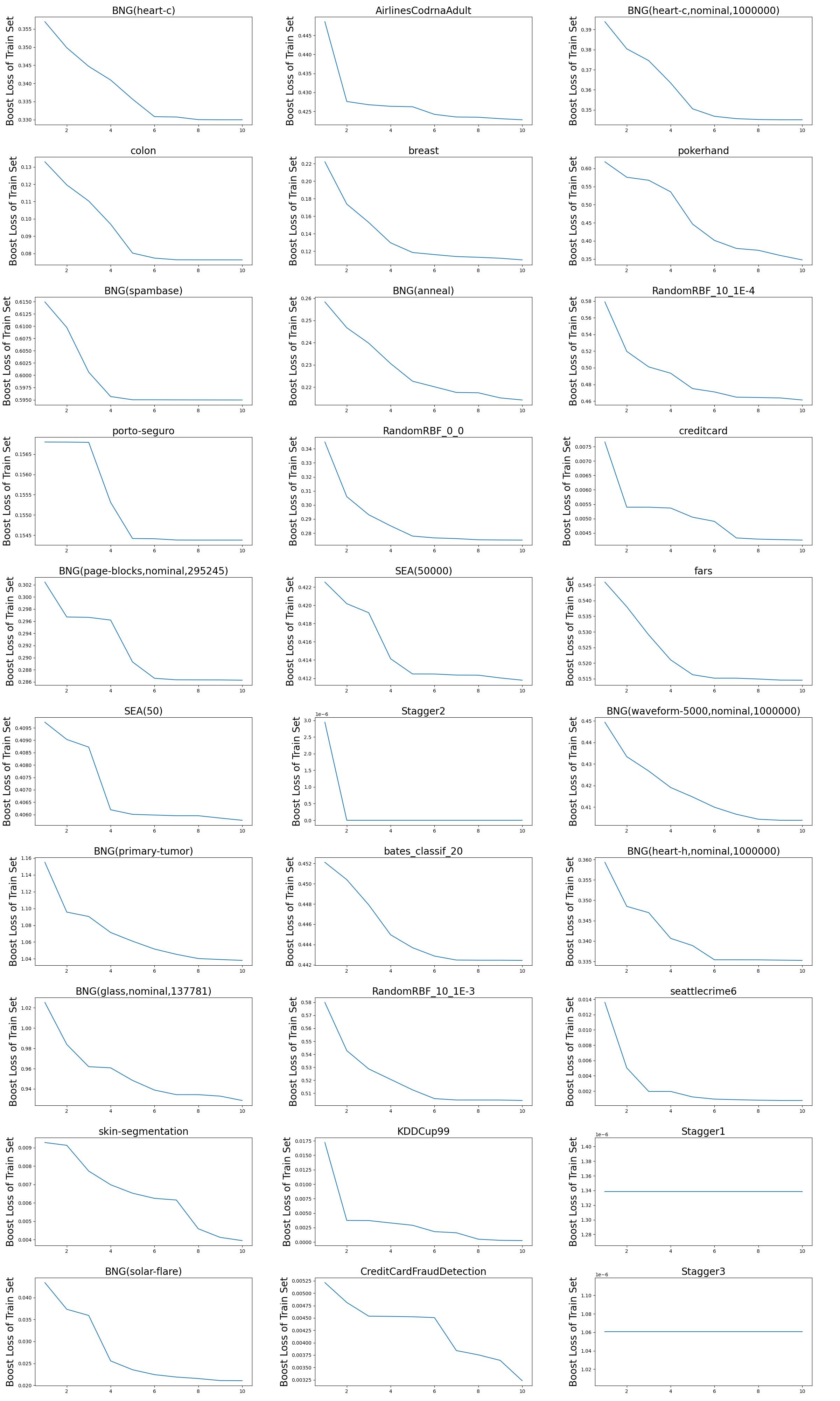
Figure 4: Boost loss on training set for all large datasets with 10 weak learners.

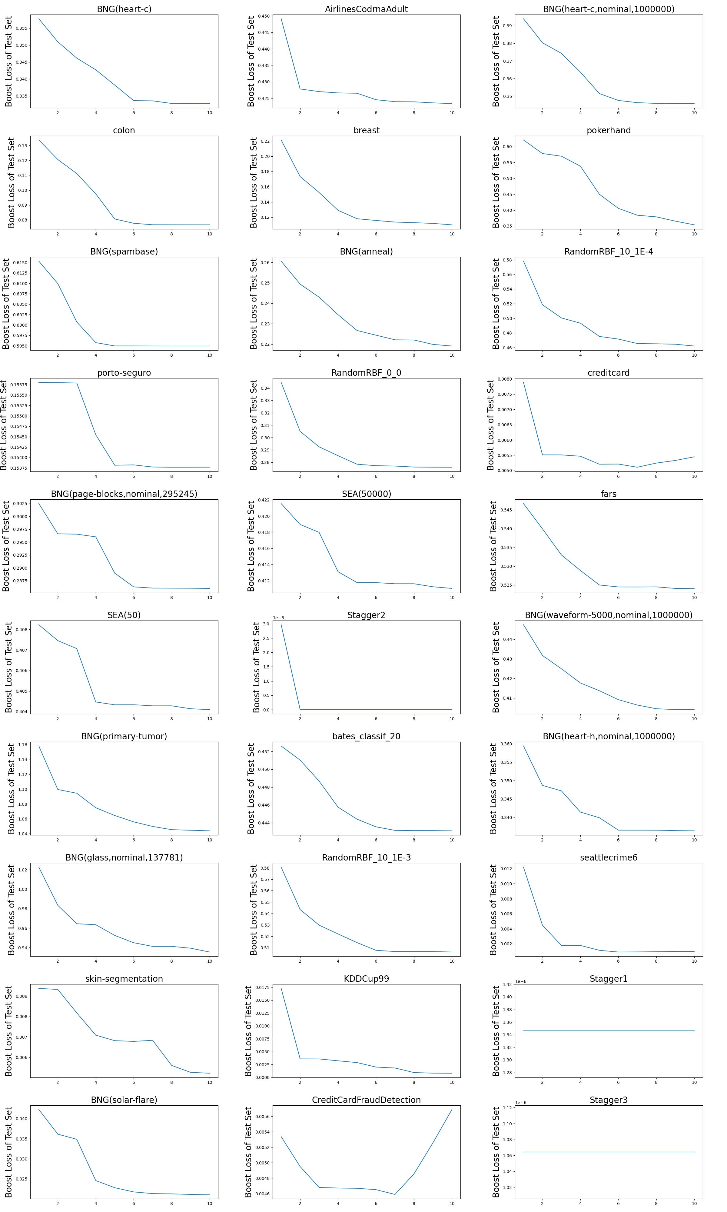
Figure 5: Boost loss on test set for all large datasets with 10 weak learners.

References

- [1] Sercan Ö Arik and Tomas Pfister. Tabnet: Attentive interpretable tabular learning. In Proceedings of the AAAI conference on artificial intelligence, volume 35, pages 6679–6687, 2021.
- [2] Iz Beltagy, Matthew E. Peters, and Arman Cohan. Longformer: The long-document transformer, 2020.
- [3] Omar Benjelloun, Shiyu Chen, and Natasha Noy. Google dataset search by the numbers. In International Semantic Web Conference, pages 667–682. Springer, 2020.
- [4] Bernd Bischl, Giuseppe Casalicchio, Matthias Feurer, Pieter Gijsbers, Frank Hutter, Michel Lang, Rafael Gomes Mantovani, Jan N van Rijn, and Joaquin Vanschoren. Openml benchmarking suites. In Proceedings of the NeurIPS 2021 Datasets and Benchmarks Track. 2021.
- [5] Vadim Borisov, Tobias Leemann, Kathrin Seßler, Johannes Haug, Martin Pawelczyk, and Gjergji Kasneci. Deep neural networks and tabular data: A survey. IEEE Transactions on Neural Networks and Learning Systems, 2022.
- [6] Leo Breiman. Bagging predictors. Machine learning, 24:123–140, 1996.
- [7] Tianqi Chen and Carlos Guestrin. Xgboost: A scalable tree boosting system. In Proceedings of the 22nd acm sigkdd international conference on knowledge discovery and data mining, pages 785–794, 2016.
- [8] Rewon Child, Scott Gray, Alec Radford, and Ilya Sutskever. Generating long sequences with sparse transformers, 2019.
- [9] Jillian M Clements, Di Xu, Nooshin Yousefi, and Dmitry Efimov. Sequential deep learning for credit risk monitoring with tabular financial data. arXiv preprint arXiv:2012.15330, 2020.
- [10] Allison McCarn Deiana, Nhan Tran, Joshua Agar, Michaela Blott, Giuseppe Di Guglielmo, Javier Duarte, Philip Harris, Scott Hauck, Mia Liu, Mark S Neubauer, et al. Applications and techniques for fast machine learning in science. Frontiers in big Data, 5:787421, 2022.
- [11] Nick Erickson, Jonas Mueller, Alexander Shirkov, Hang Zhang, Pedro Larroy, Mu Li, and Alexander Smola. Autogluon-tabular: Robust and accurate automl for structured data. arXiv preprint arXiv:2003.06505, 2020.
- [12] Andre Esteva, Alexandre Robicquet, Bharath Ramsundar, Volodymyr Kuleshov, Mark DePristo, Katherine Chou, Claire Cui, Greg Corrado, Sebastian Thrun, and Jeff Dean. A guide to deep learning in healthcare. Nature medicine, 25(1):24–29, 2019.
- [13] Matthias Feurer, Katharina Eggensperger, Stefan Falkner, Marius Lindauer, and Frank Hutter. Auto-sklearn 2.0: Hands-free automl via meta-learning. The Journal of Machine Learning Research, 23(1):11936–11996, 2022.
- [14] Jerome H Friedman. Greedy function approximation: a gradient boosting machine. Annals of statistics, pages 1189–1232, 2001.
- [15] Jerome H Friedman. Stochastic gradient boosting. Computational statistics & data analysis, 38(4):367–378, 2002.
- [16] Yury Gorishniy, Ivan Rubachev, Valentin Khrulkov, and Artem Babenko. Revisiting deep learning models for tabular data. Advances in Neural Information Processing Systems, 34:18932–18943, 2021.
- [17] Léo Grinsztajn, Edouard Oyallon, and Gaël Varoquaux. Why do tree-based models still outperform deep learning on typical tabular data? Advances in Neural Information Processing Systems, 35:507–520, 2022.
- [18] Qipeng Guo, Xipeng Qiu, Pengfei Liu, Yunfan Shao, Xiangyang Xue, and Zheng Zhang. Star-transformer. In Proceedings of HLT-NAACL, pages 1315–1325, 2019.
- [19] Trevor Hastie, Saharon Rosset, Ji Zhu, and Hui Zou. Multi-class adaboost. Statistics and its Interface, 2(3):349–360, 2009.
- [20] Trevor Hastie, Robert Tibshirani, Jerome H Friedman, and Jerome H Friedman. The elements of statistical learning: data mining, inference, and prediction, volume 2. Springer, 2009.
- [21] Noah Hollmann, Samuel Müller, Katharina Eggensperger, and Frank Hutter. TabPFN: A transformer that solves small tabular classification problems in a second. In The Eleventh International Conference on Learning Representations, 2023.
- [22] Noah Hollmann, Samuel Müller, Lennart Purucker, Arjun Krishnakumar, Max Körfer, Shi Bin Hoo, Robin Tibor Schirrmeister, and Frank Hutter. Accurate predictions on small data with a tabular foundation model. Nature, 637(8045):319–326, 2025.
- [23] Bairu Hou, Joe O’connor, Jacob Andreas, Shiyu Chang, and Yang Zhang. Promptboosting: Black-box text classification with ten forward passes. In International Conference on Machine Learning, pages 13309–13324. PMLR, 2023.
- [24] Gautier Izacard, Mathilde Caron, Lucas Hosseini, Sebastian Riedel, Piotr Bojanowski, Armand Joulin, and Edouard Grave. Unsupervised dense information retrieval with contrastive learning. Transactions on Machine Learning Research, 2022.
- [25] Arlind Kadra, Marius Lindauer, Frank Hutter, and Josif Grabocka. Well-tuned simple nets excel on tabular datasets. Advances in neural information processing systems, 34:23928–23941, 2021.
- [26] Vladimir Karpukhin, Barlas Oğuz, Sewon Min, Patrick Lewis, Ledell Wu, Sergey Edunov, Danqi Chen, and Wen tau Yih. Dense passage retrieval for open-domain question answering, 2020.
- [27] Guolin Ke, Qi Meng, Thomas Finley, Taifeng Wang, Wei Chen, Weidong Ma, Qiwei Ye, and Tie-Yan Liu. Lightgbm: A highly efficient gradient boosting decision tree. Advances in neural information processing systems, 30, 2017.
- [28] Omar Khattab and Matei Zaharia. Colbert: Efficient and effective passage search via contextualized late interaction over bert, 2020.
- [29] Jannik Kossen, Neil Band, Clare Lyle, Aidan N Gomez, Thomas Rainforth, and Yarin Gal. Self-attention between datapoints: Going beyond individual input-output pairs in deep learning. Advances in Neural Information Processing Systems, 34:28742–28756, 2021.
- [30] Xiaonan Li, Changtai Zhu, Linyang Li, Zhangyue Yin, Tianxiang Sun, and Xipeng Qiu. Llatrieval: Llm-verified retrieval for verifiable generation, 2023.
- [31] Haihao Lu and Rahul Mazumder. Randomized gradient boosting machine, 2020.
- [32] Hariharan Manikandan, Yiding Jiang, and J Zico Kolter. Language models are weak learners, 2023.
- [33] Samuel Müller, Noah Hollmann, Sebastian Pineda Arango, Josif Grabocka, and Frank Hutter. Transformers can do bayesian inference. In International Conference on Learning Representations, 2021.
- [34] Thomas Nagler. Statistical foundations of prior-data fitted networks. In Andreas Krause, Emma Brunskill, Kyunghyun Cho, Barbara Engelhardt, Sivan Sabato, and Jonathan Scarlett, editors, Proceedings of the 40th International Conference on Machine Learning, volume 202 of Proceedings of Machine Learning Research, pages 25660–25676. PMLR, 23–29 Jul 2023.
- [35] Rodrigo Nogueira, Wei Yang, Jimmy Lin, and Kyunghyun Cho. Document expansion by query prediction, 2019.
- [36] Liudmila Prokhorenkova, Gleb Gusev, Aleksandr Vorobev, Anna Veronika Dorogush, and Andrey Gulin. Catboost: unbiased boosting with categorical features. Advances in neural information processing systems, 31, 2018.
- [37] Anand Rajaraman and Jeffrey David Ullman. Data Mining, page 1–17. Cambridge University Press, 2011.
- [38] S. Robertson. The Probabilistic Relevance Framework: BM25 and Beyond. Foundations and Trends® in Information Retrieval, 3(4):333–389, 2009.
- [39] Matthias Seeger. Gaussian processes for machine learning. International journal of neural systems, 14(02):69–106, 2004.
- [40] Weijia Shi, Sewon Min, Michihiro Yasunaga, Minjoon Seo, Rich James, Mike Lewis, Luke Zettlemoyer, and Wen tau Yih. Replug: Retrieval-augmented black-box language models, 2023.
- [41] Ravid Shwartz-Ziv and Amitai Armon. Tabular data: Deep learning is not all you need, 2021.
- [42] Ravid Shwartz-Ziv and Amitai Armon. Tabular data: Deep learning is not all you need. Information Fusion, 81:84–90, 2022.
- [43] Gowthami Somepalli, Micah Goldblum, Avi Schwarzschild, C Bayan Bruss, and Tom Goldstein. Saint: Improved neural networks for tabular data via row attention and contrastive pre-training. arXiv preprint arXiv:2106.01342, 2021.
- [44] Hongjin Su, Weijia Shi, Jungo Kasai, Yizhong Wang, Yushi Hu, Mari Ostendorf, Wen tau Yih, Noah A. Smith, Luke Zettlemoyer, and Tao Yu. One embedder, any task: Instruction-finetuned text embeddings, 2023.
- [45] Qi Tang, Guoen Xia, Xianquan Zhang, and Feng Long. A customer churn prediction model based on xgboost and mlp. In 2020 International Conference on Computer Engineering and Application (ICCEA), pages 608–612. IEEE, 2020.
- [46] Dennis Ulmer, Lotta Meijerink, and Giovanni Cinà. Trust issues: Uncertainty estimation does not enable reliable ood detection on medical tabular data. In Machine Learning for Health, pages 341–354. PMLR, 2020.
- [47] Christopher J Urban and Kathleen M Gates. Deep learning: A primer for psychologists. Psychological Methods, 26(6):743, 2021.
- [48] Yuxin Wang, Chu-Tak Lee, Qipeng Guo, Zhangyue Yin, Yunhua Zhou, Xuanjing Huang, and Xipeng Qiu. What dense graph do you need for self-attention? In Kamalika Chaudhuri, Stefanie Jegelka, Le Song, Csaba Szepesvari, Gang Niu, and Sivan Sabato, editors, Proceedings of the 39th International Conference on Machine Learning, volume 162 of Proceedings of Machine Learning Research, pages 22752–22768. PMLR, 17–23 Jul 2022.
- [49] Canwen Xu, Daya Guo, Nan Duan, and Julian McAuley. Laprador: Unsupervised pretrained dense retriever for zero-shot text retrieval, 2022.
- [50] Manzil Zaheer, Guru Guruganesh, Avinava Dubey, Joshua Ainslie, Chris Alberti, Santiago Ontanon, Philip Pham, Anirudh Ravula, Qifan Wang, Li Yang, and Amr Ahmed. Big bird: Transformers for longer sequences, 2021.
- [51] Yuyu Zhang, Ping Nie, Xiubo Geng, Arun Ramamurthy, Le Song, and Daxin Jiang. Dc-bert: Decoupling question and document for efficient contextual encoding, 2020.