Constraints on the inflaton potential from scalar-induced gravitational waves and primordial black holes

Abstract

A plateau on the background inflaton potential $V_{\rm b}(\phi)$ can lead cosmic inflation into an ultraslow-roll phase, greatly enhancing the primordial power spectrum on small scales, and resulting in significant scalar-induced gravitational waves (GWs) and abundant primordial black holes (PBHs). In this work, we construct an anti-symmetric perturbation $\delta V(\phi)$ on $V_{\rm b}(\phi)$ with three model parameters, the position, width, and slope of $\delta V(\phi)$, and constrain these parameters from the potential stochastic gravitational wave background (SGWB) in NANOGrav 15-year data set. The GW spectrum from the merger of supermassive black hole binaries (SMBHBs) with two model parameters, the amplitude and spectral index, is also investigated for comparison. We perform Bayesian analysis in three steps with increasing number of model parameters, and obtain the allowed parameter ranges. When the constraints on PBH abundance are taken into account, these ranges become further narrower. We find that the increase of model parameters cannot significantly improve the Bayes factors, and the model with an almost perfect plateau on $V_{\rm b}(\phi)$ is favored. Moreover, the interpretation of the SGWB via only the GWs generated by SMBHBs is not preferred by the data.

1 Introduction

The detection of the gravitational waves (GWs) from the merger of black hole binaries (BHBs) has marked the beginning of a new epoch in modern cosmology LIGOScientific:2016aoc ; KAGRA:2021vkt . GWs offer a new tool for probing the early Universe and present the insights beyond the reach of traditional electromagnetic observations. GWs may have various origins, such as cosmological phase transitions Caprini:2015zlo ; Hindmarsh:2020hop and topological defects Martin:1996ea ; Figueroa:2012kw ; Saikawa:2017hiv ; Gouttenoire:2023ftk , and can also be induced by scalar perturbations Baumann:2007zm ; Bugaev:2009zh ; Espinosa:2018eve ; Kohri:2018awv ; Ragavendra:2020sop ; Ragavendra:2023ret ; Das:2023nmm . These different sources collectively contribute to the stochastic GW background (SGWB), which provides crucial information for understanding astrophysics and cosmology. Therefore, the observation of the SGWB is the primary goal of various GW detectors that are designed for these faint but informative signals from a wide range of cosmic events.

The recent observations from the European Pulsar Timing Array (EPTA) EPTA:2023fyk , Parkes PTA Zic:2023gta , Chinese PTA Xu:2023wog , North American Nanohertz Observatory for Gravitational Waves (NANOGrav) NANOGrav:2023gor ; NANOGrav:2023hvm , and Meerkat PTA Miles:2024rjc have provided multiple pieces of evidence for an excess of the signals at low frequencies with respect to the Hellings–Downs correlations Hellings:1983fr , supporting the potential existence of the SGWB. In this work, we attribute the SGWB to the scalar-induced GWs (SIGWs), which are the second-order effects of the first-order scalar perturbations generated during cosmic inflation. If these scalar perturbations are large enough on small scales, they can also produce a significant number of primordial black holes (PBHs) at the same time. These PBHs can explain a portion of the BHB merger events, serve as the seeds of supermassive black holes at galactic centers, and more importantly, are a natural candidate of dark matter (DM). For more recent researches on the PTA observations and the related topics on SIGWs and PBHs, see Refs. Ashoorioon:2022raz ; Franciolini:2023pbf ; Ellis:2023oxs ; Gangopadhyay:2023qjr ; Chang:2023vjk ; Iovino:2024sgs ; Allegrini:2024ooy ; Wu:2024qdb and the references therein.

Usually, the single-field slow-roll (SR) inflation models lead to a nearly scale-invariant power spectrum of scalar perturbations, confirmed by the measurements of the cosmic microwave background anisotropies on large scales Planck:2018jri . However, the SIGWs from such a power spectrum are too weak to account for the SGWB. To have sufficiently large SIGWs, we need to break the SR conditions by imposing a period of ultraslow-roll (USR) phase in cosmic inflation. This approach allows us to significantly amplify the power spectrum on small scales, generating intensive SIGWs and producing abundant PBHs simultaneously. There are many mechanisms for the USR inflation, which can be realized by a (near-)inflection point on the inflaton potential Germani:2017bcs ; Dimopoulos:2017ged ; Di:2017ndc ; Ashoorioon:2020hln , in modified gravity theories Pi:2017gih ; Lin:2020goi ; Saburov:2024und , or in supergravity models Wu:2021zta ; Ishikawa:2021xya ; Ishikawa:2024xjp , etc. For a comprehensive introduction to the USR inflation, see Refs. Ezquiaga:2017fvi ; Cicoli:2018asa ; Dalianis:2018frf ; Cheng:2018qof ; Mishra:2019pzq ; Kefala:2020xsx ; Wu:2021mwy ; Hooshangi:2022lao ; Franciolini:2022pav ; Gu:2022pbo ; Mu:2022dku . In this paper, following our previous works in Refs. Wang:2021kbh ; Liu:2021qky ; Zhao:2023xnh ; Zhao:2023zbg ; Zhao:2024yzg ; Su:2025mam , we consider an anti-symmetric perturbation $\delta V(\phi)$ on the background inflaton potential to realize the USR phase.

Our goal in this work is to determine the position, width, and amplitude of $\delta V(\phi)$ by the constraints from the SIGW spectrum and the PBH abundance. First, we adopt the NANOGrav 15-year data set, utilize a modified version of the SIGWfast code Witkowski:2022mtg to compute the SIGW spectrum, and perform Bayesian analysis Thrane:2018qnx by the PTArcade code Mitridate:2023oar . Second, the model parameters extracted from the SIGW spectrum must lead to reasonable PBH abundance in relevant mass range at the same time, and this demand will further shrink the allowed parameter ranges. Third, as there is also possibility that the SGWB are generated from supermassive black hole binaries (SMBHBs) NANOGrav:2023gor ; NANOGrav:2023hvm , we need to consider the scenario that the SGWB origins from both SIGWs and SMBHBs. These three points will constitute the main content of our work. More importantly, we do not assume any simple form of the primordial power spectrum as done in many previous works, but constrain the model parameters of the inflaton potential directly from the GW data. This operation is also supported by Ref. LISACosmologyWorkingGroup:2025vdz , where the authors studied different methods (template based, agnostic, and ab initio) to constrain the USR phase, and found that using the explicit USR construction leads to the minimum residuals.

This paper is organized as follows. In Sec. 2, we introduce the inflaton potential, show the power spectrum of the primordial curvature perturbation, and calculate the PBH abundance. In Sec. 3, we derive the SIGW spectrum. The NANOGrav 15-year data set and the relevant Bayesian analysis method are reviewed in Sec. 4. With all these preparations, we constrain our inflation model in Sec. 5, with two model parameters, three model parameters, and SMBHBs taken into account, respectively. The Bayes factors between different models are also calculated and discussed in detail. We conclude in Sec. 6. We work in the natural system of units and set $c=\hbar=k_{\mathrm{B}}=1$.

2 USR inflation and PBHs

In this section, we discuss the equation of motion for the primordial curvature perturbation $\mathcal{R}$, introduce its power spectrum ${\cal P}_{\mathcal{R}}(k)$, and show the calculation of PBH abundance $f_{\rm PBH}$.

2.1 Basic equations

First, the action of the single-field inflation reads

$$S=\int\mathrm{d}^{4}x\,\sqrt{-g}\left[\frac{m_{\text{P}}^{2}}{2}R-\frac{1}{2}\partial_{\mu}\phi\partial^{\mu}\phi-V(\phi)\right],$$

where $m_{\rm P}=1/\sqrt{8\pi G}$ is the reduced Planck mass, $R$ is the Ricci scalar, $\phi$ is the inflaton field, and $V(\phi)$ is its potential, respectively. By variation of $S$, the equation of motion for $\phi$ can be obtained as the Klein–Gordon equation,

$$\ddot{\phi}+3H\dot{\phi}+V_{,\phi}=0,$$ (1)

where $H$ is Hubble expansion rate.

During inflation, it is more convenient to use the number of $e$-folds $N$ to describe cosmic expansion, defined as $\mathrm{d}N=H(t)\,\mathrm{d}t=\mathrm{d}\ln{a}(t)$, where $t$ is the cosmic time, $a(t)$ is the scale factor, and $H=\dot{a}/a$. In addition, to characterize the SR behaviors of the inflaton, two SR parameters can be introduced as

$$\varepsilon =-\frac{\dot{H}}{H^{2}}=\frac{\phi_{,N}^{2}}{2m_{\mathrm{P}}^{2}},\quad\eta=-\frac{\ddot{\phi}}{H\dot{\phi}}=\frac{\phi_{,N}^{2}}{2m_{\mathrm{P}}^{2}}-\frac{\phi_{,NN}}{\phi_{,N}}.$$ (2)

With these parameters, Eq. (1) can be reexpressed as

$$\phi_{,NN}+(3-\varepsilon)\phi_{,N}+\frac{1}{H^{2}}V_{,\phi}=0,$$

and the Friedmann equation for cosmic expansion can be written as

$$H^{2}=\frac{V}{(3-\varepsilon)m_{\rm P}^{2}}.$$

Then, we move on to the perturbations on the background spacetime. In Newtonian gauge, the perturbed metric is given as

$$\mathrm{d}s^{2} =-(1+2\Psi)\,\mathrm{d}t^{2}+a^{2}(t)\left[(1-2\Psi)\delta_{ij}+\frac{1}{2}h_{ij}\right]\,\mathrm{d}x^{i}\mathrm{d}x^{j},$$ (3)

where $\Psi$ is the first-order scalar perturbation, $h_{ij}$ is the second-order tensor perturbation, and we have neglected the vector perturbation and anisotropic stress here. A more frequently used gauge-invariant scalar perturbation is the primordial curvature perturbation $\mathcal{R}$,

$$\mathcal{R}=\Psi+\frac{H}{\dot{\phi}}\,\delta\phi,$$

where $\delta\phi$ is the perturbation of the inflaton field. The equation of motion for the Fourier mode $\mathcal{R}_{k}$ is the Mukhanov–Sasaki equation Sasaki:1983kd ; Mukhanov ,

$$\mathcal{R}_{k,NN}+(3+\varepsilon-2\eta)\mathcal{R}_{k,N}+\frac{k^{2}}{H^{2}e^{2N}}\mathcal{R}_{k}=0.$$ (4)

2.2 Inflaton potential

The Fourier mode $\mathcal{R}_{k}$ can be obtained by numerically solving Eqs. (1), (2), and (4), which requires us to specify the form of the inflaton potential $V(\phi)$. In this work, following our previous works in Refs. Wang:2021kbh ; Liu:2021qky ; Zhao:2023xnh ; Zhao:2023zbg ; Zhao:2024yzg ; Su:2025mam , we decompose $V(\phi)$ as a sum of its background $V_{\mathrm{b}}(\phi)$ and a perturbation $\delta V(\phi)$ on it,

$$V(\phi)=V_{\mathrm{b}}(\phi)+\delta V(\phi).$$

First, the background potential $V_{\mathrm{b}}(\phi)$ is adopted as the Kachru–Kallosh–Linde–Trivedi potential Kachru:2003aw ,

$$V_{\rm b}(\phi)=V_{0}\frac{\phi^{2}}{\phi^{2}+(m_{\mathrm{P}}/2)^{2}},$$

where $V_{0}$ describes the energy scale of inflation. Then, we parameterize the perturbation $\delta V(\phi)$ in an anti-symmetric form as

$$\delta V(\phi)=-AV_{0}(\phi-\phi_{0})\exp\left[-\frac{(\phi-\phi_{0})^{2}}{2\sigma^{2}}\right],$$ (5)

where $A$, $\phi_{0}$, and $\sigma$ are three model parameters that determine the amplitude, position, and width of $\delta V(\phi)$, respectively. For convenience, we reexpress $A$ as

$$A=V_{\text{b},\phi}(\phi_{0})(1+A_{0}).$$ (6)

By this means, $A_{0}$ characterizes the deviation of $V(\phi)$ from a perfect plateau at $\phi_{0}$. Moreover, we set $V_{0}/m^{4}_{\text{P}}=10^{-10}$, $\phi_{\rm i}/m_{\text{p}}=3.30$, and $\phi_{{\rm i},N}/m_{\text{P}}=-0.0137$ as the initial conditions for inflation, such that there can be a nearly scale-invariant power spectrum and a relatively small tensor-to-scalar ratio favored by the cosmic microwave background observations on large scales Planck:2018jri .

2.3 Power spectra and PBH abundance

To obtain the PBH abundance, we introduce the dimensionless power spectrum $\mathcal{P}{{}_{\mathcal{R}}}(k)$ of ${\cal R}_{k}$,

$$\mathcal{P}_{\mathcal{R}}(k)=\frac{k^{3}}{2\pi^{2}}|\mathcal{R}_{k}|^{2}\bigg{|}_{k\ll aH}.$$ (7)

Here, we should emphasize that, as ${\cal R}_{k}$ can still evolve after crossing the Hubble horizon during the USR inflation, $\mathcal{P}_{\mathcal{R}}(k)$ must be evaluated at the end of inflation, with the relevant scale satisfying $k\ll aH$.

Furthermore, we need to link $\mathcal{P}_{\mathcal{R}}(k)$ to the dimensionless power spectrum $\mathcal{P}_{\delta}(k)$ of the primordial density contrast $\delta$. In the radiation-dominated (RD) era, at the linear order, we have Green:2004wb

$$\mathcal{P}_{\delta}(k)=\frac{16}{81}\left(\frac{k}{aH}\right)^{4}\mathcal{P}_{\mathcal{R}}(k).$$

By this relation, the $i$-th spectral moment $\sigma_{i}$ of the density contrast $\delta$ can be obtained as

$$\sigma_{i}^{2}(R) =\int_{0}^{\infty}\frac{\mathrm{d}k}{k}\,k^{2i}\widetilde{W}^{2}(k,R)\mathcal{P}_{\delta}(k)=\frac{16}{81}\int_{0}^{\infty}\frac{\mathrm{d}k}{k}\,k^{2i}\widetilde{W}^{2}(k,R)(kR)^{4}\mathcal{P}_{\mathcal{R}}(k).$$ (8)

where $i=0,1,2,\cdots$, and $\widetilde{W}(k,R)$ is the window function in the Fourier space, which smooths the perturbation over some physical scale $R$, often chosen as $R=1/(aH)$. In this work, we choose Gaussian window function as $\widetilde{W}^{2}(k,R)=e^{-k^{2}R^{2}/2}$, which prevents the issues related to the non-differentiability and divergence of the integral in the large-$k$ limit in Eq. (8).

For PBH formation, in the Carr–Hawking collapse model Carr:1974nx , the PBH mass $M$ is related to the horizon mass $M_{\mathrm{H}}$ as

$$M=\kappa M_{\mathrm{H}}=\kappa\frac{4\pi m^{2}_{\text{P}}}{H},$$

where $\kappa$ is the collapse efficiency. Considering the conservation of entropy in the adiabatic cosmic expansion, we can obtain Carr:2020gox

$$\frac{M}{M_{\odot}}=1.13\times 10^{15}\left(\frac{\kappa}{0.2}\right)\left(\frac{g_{*}}{106.75}\right)^{-1/6}\left(\frac{k_{*}}{k_{\mathrm{PBH}}}\right)^{2},$$ (9)

where $M_{\odot}=1.99\times 10^{30}$ kg is the solar mass, $g_{*}$ is the effective number of relativistic degrees of freedom of energy density, $k_{*}=0.05~\text{Mpc}^{-1}$ is the cosmic microwave background pivot scale for the Planck satellite experiment Planck:2018jri , and $k_{\text{PBH}}=1/R$ is the wave number of the PBH that exits the Hubble horizon. Below, we set $\kappa=0.2$ and $g_{*}=106.75$ in the RD era Carr:1975qj . From Eq. (9), all spectral moments $\sigma_{i}(R)$ can be reexpressed in terms of the PBH mass as $\sigma_{i}(M)$.

At the epoch of PBH formation in the RD era, its mass fraction $\beta_{\rm{PBH}}(M)$ is defined as

$$\left.\beta_{\mathrm{PBH}}(M)=\frac{\rho_{\mathrm{PBH}}(M)}{\rho_{\mathrm{R}}}\right|_{\rm formation},$$

where $\rho_{\mathrm{PBH}}(M)$ and $\rho_{\mathrm{R}}$ are the energy densities of PBH and radiation. Then, at the present time, the PBH abundance $f_{\rm PBH}(M)$ is defined as

$$f_{\mathrm{PBH}}(M)=\left.\frac{\rho_{\mathrm{PBH}}(M)}{\rho_{\mathrm{DM}}}\right|_{\rm today},$$

where $\rho_{\mathrm{DM}}$ is the energy density of DM. If we focus on monochromatic PBH mass, $f_{\mathrm{PBH}}(M)$ is naturally proportional to $\beta_{\mathrm{PBH}}(M)$,

$$f_{\mathrm{PBH}}(M)=1.68\times 10^{8}\left(\frac{M}{M_{\odot}}\right)^{-1/2}\beta_{\mathrm{PBH}}(M).$$

The PBH mass fraction $\beta_{\mathrm{PBH}}(M)$ can be calculated in different ways, corresponding to taking the spectral moments $\sigma_{i}$ at different orders. In the general peak theory Bardeen:1985tr , all $\sigma_{0}$, $\sigma_{1}$, and $\sigma_{2}$ are needed, but the relevant calculations are rather tedious. A very convenient and effective simplification is the Green–Liddle–Malik–Sasaki (GLMS) approximation Green:2004wb , which only consults $\sigma_{0}$ and $\sigma_{1}$ but yields almost the same results as peak theory. Hence, in this work, we will follow the GLMS method, which gives

$$\beta_{\text{PBH}}(M)=\frac{1}{\sqrt{2\pi}}Q^{3}(\nu_{\rm c}^{2}-1)e^{-\nu_{\rm c}^{2}/2},$$

where $Q=R\sigma_{1}/(\sqrt{3}\sigma_{0})$, $\nu_{\text{c}}=\delta_{\text{c}}/\sigma_{0}$ is the relative density contrast, and $\delta_{\rm c}$ is the threshold of $\delta$ for PBH formation, which depends on many physical issues, such as the shape of the collapsing region Musco:2018rwt , and the equation of state and the anisotropy of the cosmic medium Harada:2013epa ; Escriva:2019nsa ; Musco:2020jjb ; Musco:2021sva ; Papanikolaou:2022cvo ; Stamou:2023vxu . In this work, we follow Ref. Harada:2013epa and choose $\delta_{\rm c}=0.414$.

3 SIGWs

In this section, we provide a concise review of the derivation of the SIGW spectra in the RD era and at the present time.

3.1 Basic equations

The equation of motion for the second-order tensor perturbation $h_{ij}$ in Eq. (3) reads Baumann:2007zm

$$h_{ij}^{\prime\prime}+2\mathcal{H}h_{ij}^{\prime}-\nabla^{2}h_{ij}=-4{\mathcal{T}}_{ij}^{lm}\mathcal{S}_{lm},$$ (10)

where ${\mathcal{T}}_{ij}^{lm}$ is the projection operator, $\mathcal{S}_{lm}$ is the source term, a prime denotes the derivative with respect to the conformal time $\tau$ defined as $\mathrm{d}\tau=\mathrm{d}t/a(t)$, and ${\cal H}=a^{\prime}/a$. In the RD era, using the conformal Newtonian gauge, we have

$$\mathcal{S}_{ij} =4\Psi\partial_{i}\partial_{j}\Psi+2\partial_{i}\Psi\partial_{j}\Psi-\frac{1}{\mathcal{H}^{2}}\partial_{i}(\Psi^{\prime}+\mathcal{H}\Psi)\partial_{j}(\Psi^{\prime}+\mathcal{H}\Psi).$$

In general, the Fourier transform of $h_{ij}$ is

$$h_{ij}(\tau,\mathbf{x})=\int\frac{\mathrm{d}^{3}k}{(2\pi)^{3/2}}\,e^{i\mathbf{k}\cdot\mathbf{x}}[h_{\mathbf{k}}^{+}(\tau){e}_{ij}^{+}(\mathbf{k})+h_{\mathbf{k}}^{\times}(\tau){e}_{ij}^{\times}(\mathbf{k})],$$

where $h_{\mathbf{k}}^{+}(\tau)$ and $h_{\mathbf{k}}^{\times}(\tau)$ are the Fourier components of $h_{ij}(\tau,{\bf x})$, and ${e}_{ij}^{+}(\mathbf{k})$ and ${e}_{ij}^{\times}(\mathbf{k})$ are two time-independent polarization tensors that can be expressed in terms of two orthogonal basis vectors $\mathbf{e}$ and $\bar{\mathbf{e}}$ as

$${e}_{ij}^{+}(\mathbf{k}) =\frac{1}{\sqrt{2}}\left[{e}_{i}(\mathbf{k}){e}_{j}(\mathbf{k})-\overline{{e}}_{i}(\mathbf{k})\overline{{e}}_{j}(\mathbf{k})\right],\quad{e}_{ij}^{\times}(\mathbf{k})=\frac{1}{\sqrt{2}}\left[{e}_{i}(\mathbf{k})\overline{{e}}_{j}(\mathbf{k})+\overline{{e}}_{i}(\mathbf{k}){e}_{j}(\mathbf{k})\right].$$

In the Fourier space, Eq. (10) becomes

$$h^{\prime\prime}_{\mathbf{k}}+2\mathcal{H}h^{\prime}_{\mathbf{k}}+k^{2}h_{\mathbf{k}}=\mathcal{S}(\tau,\mathbf{k}),$$ (11)

where $\mathcal{S}(\tau,\mathbf{k})$ is the Fourier transform of the source term $\mathcal{S}_{ij}(\tau,\mathbf{x})$, and we have ignored the polarization indices $+$ and $\times$. Furthermore, we decompose the Fourier mode of the scalar perturbation $\Psi$ as $\Psi_{\mathbf{k}}(\tau)=\Psi(k\tau)\psi_{\mathbf{k}}$, where $\psi_{\mathbf{k}}$ is the initial value, and $\Psi(k\tau)$ is the normalized transfer function. In the RD era, we have Kohri:2018awv

$$\Psi(k\tau)=\frac{9}{(k\tau)^{2}}\left[\frac{\sin(k\tau/\sqrt{3})}{k\tau/\sqrt{3}}-\cos(k\tau/\sqrt{3})\right].$$

In this way, the source term can be reexpressed as

$${\cal S}(\tau,\mathbf{k})=\int\frac{\mathrm{d}^{3}k}{(2\pi)^{3/2}}\,{e}^{ij}(\mathbf{k})\widetilde{k}_{i}\widetilde{k}_{j}f(\tau,\mathbf{k},\widetilde{\mathbf{k}})\psi_{\mathbf{k}}\psi_{\mathbf{k}-\widetilde{\mathbf{k}}},$$

where the source function $f(\tau,\mathbf{k},\widetilde{\mathbf{k}})$ is Domenech:2021ztg

$$f(\tau,{\bf k},\widetilde{\bf k}) =12\Psi(|\widetilde{\mathbf{k}}|\tau)\Psi(|\mathbf{k}-\widetilde{\bf k}|\tau)+4\tau^{2}\Psi^{\prime}(|\widetilde{\mathbf{k}}|\tau)\Psi^{\prime}(|\mathbf{k}-\widetilde{\mathbf{k}}|\tau)$$

$$\quad+4\tau\left[\Psi^{\prime}(|\widetilde{\mathbf{k}}|\tau)\Psi(|\mathbf{k}-\widetilde{\mathbf{k}}|\tau)+\Psi(|\widetilde{\mathbf{k}}|\tau)\Psi^{\prime}(|\mathbf{k}-\widetilde{\mathbf{k}}|\tau)\right].$$

With all above preparations, we can solve Eq. (11) by the Green function method,

$$h_{\mathbf{k}}(\tau)=\frac{1}{a(\tau)}\int G_{k}(\tau,\widetilde{\tau})a(\widetilde{\tau})\mathcal{S}(\widetilde{\tau},\mathbf{k})\,\mathrm{d}\widetilde{\tau},$$

where the Green function is $G_{k}(\tau,\widetilde{\tau})=\sin{[k(\tau-\widetilde{\tau})]/k}$.

3.2 SIGW spectra

The SIGW spectrum $\Omega_{\mathrm{GW}}$ is defined as the GW energy density $\rho_{\mathrm{GW}}$ per logarithmic wave number as

$$\Omega_{\mathrm{GW}}(\tau,k)=\frac{1}{\rho_{\mathrm{c}}}\frac{\mathrm{d}\rho_{\mathrm{GW}}(\tau,k)}{\mathrm{d}\ln k},$$

where $\rho_{\mathrm{c}}$ is the critical energy density of the Universe. In the transverse–traceless gauge, $\Omega_{\rm GW}(\tau,k)$ can be written as Isaacson:1968hbi ; Isaacson:1968zza

$$\Omega_{\mathrm{GW}}(\tau,k)=\frac{1}{24}\left(\frac{k}{\mathcal{H}}\right)^{2}\overline{\mathcal{P}_{h}(\tau,k)},$$

where $\overline{(\cdots)}$ denotes the oscillation average, and $\mathcal{P}_{h}(\tau,k)$ is the dimensionless power spectrum of the tensor perturbation $h_{\mathbf{k}}$,

$$\mathcal{P}_{h}(\tau,k)=\frac{k^{3}}{2\pi^{2}}\delta_{\rm D}(\mathbf{k}+\widetilde{\mathbf{k}})\langle h_{\mathbf{k}}(\tau)h_{\widetilde{\mathbf{k}}}(\tau)\rangle,$$

where $\delta_{\rm D}$ is the Dirac $\delta$ function, and the two-point correlation function $\langle h_{\mathbf{k}}(\tau)h_{\widetilde{\mathbf{k}}}(\tau)\rangle$ reads

$$\langle h_{\mathbf{k}}(\tau)h_{\widetilde{\mathbf{k}}}(\tau)\rangle =\int\frac{\mathrm{d}^{3}q\mathrm{d}^{3}\widetilde{q}}{(2\pi)^{3}}\,e^{ij}({\bf k})e^{lm}({\widetilde{\bf k}})q_{i}q_{j}\widetilde{q}_{l}\widetilde{q}_{m}I(\tau,\mathbf{k},\mathbf{q})I(\tau,\widetilde{\mathbf{k}},\widetilde{\mathbf{q}})\langle\psi_{\mathbf{q}}\psi_{\mathbf{k}-\mathbf{q}}\psi_{\widetilde{\mathbf{q}}}\psi_{\widetilde{\mathbf{k}}-\widetilde{\mathbf{q}}}\rangle,$$ (12)

with $I(\tau,\mathbf{k},\mathbf{q})$ being the kernel function,

$$I(\tau,\mathbf{k},\mathbf{q})=\int\mathrm{d}\widetilde{\tau}\ \frac{a(\widetilde{\tau})}{a(\tau)}G_{k}(\tau,\widetilde{\tau})f(\widetilde{\tau},\mathbf{k},\mathbf{q}).$$

Furthermore, by the Wick theorem, the four-point correlation function $\langle\psi_{\mathbf{q}}\psi_{\mathbf{k}-\mathbf{q}}\psi_{\widetilde{\mathbf{q}}}\psi_{\widetilde{\mathbf{k}}-\widetilde{\mathbf{q}}}\rangle$ in Eq. (12) can be decomposed as the sum of the products of two-point correlation functions. It is convenient to introduce three dimensionless variables as $x=k\tau$, $u=|\mathbf{k}-\widetilde{\mathbf{k}}|/k$, and $v=|\widetilde{\mathbf{k}}|/k$. By this means, $\mathcal{P}_{h}(\tau,k)$ can be obtained as

$$\mathcal{P}_{h}(\tau,k) =4\int_{0}^{\infty}\mathrm{d}v\int_{|1-v|}^{1+v}\mathrm{d}u\,\left[\frac{4v^{2}-(1+v^{2}-u^{2})^{2}}{4uv}\right]^{2}\mathcal{I}^{2}(x,u,v)\mathcal{P}_{\mathcal{R}}(ku)\mathcal{P}_{\mathcal{R}}(kv),$$

where $\mathcal{I}(x,u,v)=I(\tau,\mathbf{k},\widetilde{\mathbf{k}})k^{2}$ is the kernel function in terms of the dimensionless variables $x$, $u$, and $v$ Ananda:2006af . In the RD era, the oscillation average of $\mathcal{I}^{2}(x,u,v)$ in the late-time limit of $x\rightarrow\infty$ is Kohri:2018awv

$$\overline{\mathcal{I}^{2}(x\rightarrow\infty,u,v)} =\frac{1}{2}\left[\frac{3(u^{2}+v^{2}-3)^{2}}{4u^{3}v^{3}x}\right]^{2}\Bigg{\{}\pi^{2}(u^{2}+v^{2}-3)^{2}\Theta(u+v-\sqrt{3})$$

$$\quad+\left[\left(u^{2}+v^{2}-3\right)\ln\left|\frac{3-(u+v)^{2}}{3-(u-v)^{2}}\right|-4uv\right]^{2}\Bigg{\}},$$

where $\Theta$ is the Heaviside step function. We may further define two new variables as $s=u+v$ and $t=u-v$. Taking into account $\mathcal{H}=1/\tau$ in the RD era, we obtain the SIGW spectrum $\Omega_{\mathrm{GW}}(\tau,k)$ as

$$\Omega_{\mathrm{GW}}(\tau,k) =12\int_{0}^{1}\mathrm{d}t\int_{1}^{\infty}\mathrm{d}s\,\frac{t(t^{2}-1)^{2}(s^{2}-1)^{2}(s^{2}+t^{2}-6)^{4}}{(s^{2}-t^{2})^{8}}$$

$$\quad\times\left\{\left[\ln\left|\frac{t^{2}-3}{s^{2}-3}\right|+\frac{2(s^{2}-t^{2})}{s^{2}+t^{2}-6}\right]^{2}+\pi^{2}\Theta(s-\sqrt{3})\right\}\mathcal{P}_{\mathcal{R}}\left(\frac{k}{2}(s+t)\right)\mathcal{P}_{\mathcal{R}}\left(\frac{k}{2}(s-t)\right).$$

Moreover, there is a simple relation between the wave number $k$ and the frequency $f$ of the SIGW Xu:2019bdp ,

$$f\approx 1.5\times 10^{-15}\frac{k}{\mathrm{Mpc}^{-1}}\,\mathrm{Hz}.$$

From this correspondence, we finally achieve the SIGW spectrum $\Omega_{\mathrm{GW}}(\tau,f)$ from $\Omega_{\mathrm{GW}}(\tau,k)$.

Last, the SIGW spectrum at present $\Omega_{\mathrm{GW}}(\tau_{0},f)$ can be related to $\Omega_{\mathrm{GW}}(\tau_{\rm c},f)$ as

$$\Omega_{\mathrm{GW}}(\tau_{0},f)h^{2}=\Omega_{\rm R}^{0}h^{2}\frac{g_{*}(f)}{g_{*}^{0}}\left(\frac{g_{*s}^{0}}{g_{*s}(f)}\right)^{4/3}\Omega_{\mathrm{GW}}\left(\tau_{\rm c},f\right),$$

where $\Omega_{\mathrm{R}}^{0}$ is the present energy density fraction of radiation, $g_{*}$ and $g_{*s}$ are the effective relativistic degrees of freedom that contribute to radiation energy and entropy densities, and $\tau_{\rm c}$ is some time after $\Omega_{\rm{GW}}(\tau,f)$ has become constant, as SIGWs can be regarded as a portion of radiation, so $\Omega_{\rm{GW}}(\tau_{\rm c},f)$ is an asymptotic constant during the RD era. In this work, we take the values $\Omega_{\mathrm{R}}^{0}h^{2}=4.184\times 10^{-5}$, $g_{*}^{0}=3.383$, and $g_{*s}^{0}=3.930$, respectively Saikawa:2020swg .

4 Bayesian analysis

In this section, we provide the elements of Bayesian analysis, including the likelihood function, prior and posterior distributions, and the Bayes factor between different models. The NANOGrav 15-year data set is also reviewed.

4.1 Likelihood function

The likelihood function $\mathcal{L}$ is related to the timing residual $\delta t$ of pulsars and can be expressed as Mitridate:2023oar ; NANOGrav:2023gor ; NANOGrav:2023hvm

$$\delta t=n+Fa+M\epsilon,$$ (13)

where $\delta t$, $n$, $a$, and $\epsilon$ are column vectors, and $F$ and $M$ are matrices, respectively.

In Eq. (13), $n$ is the white noise. The next term $Fa$ describes the time-correlated stochastic process, including the intrinsic pulsar red noise and the GW signals. First, $F$ is the Fourier basis matrix, composed of sines and cosines calculated from the time of arrival of the pulses with the frequency at $f_{i}=i/T_{\text{obs}}$ ($T_{\text{obs}}=16.03$ yr is the time of arrival extent). Second, $a$ is the amplitude, following a zero-mean normal distribution with the covariance matrix $\langle aa^{\rm T}\rangle=\phi$, which is given by

$$[\phi]_{(ai)(bj)}=\delta_{ij}(\Gamma_{ab}\Phi_{i}+\delta_{ab}\varphi_{a,i}).$$ (14)

In Eq. (14), the subscripts $a$ and $b$ correspond to the pulsars, $i$ and $j$ represent the frequency harmonics, $\Gamma_{ab}$ is the GW background overlap reduction function, denoting the mean correlation between pulsars $a$ and $b$ based on their angular separation in the sky, and the model-dependent coefficients $\Phi_{i}$ can be related to the GW spectrum as

$$\Omega_{\mathrm{GW}}(f)h^{2}=\frac{h^{2}}{\rho_{\rm c}}\frac{{\rm d}\rho_{\mathrm{GW}}(f)}{{\rm d}\ln f}=\frac{8\pi^{4}f^{5}}{H_{0}^{2}/h^{2}}\frac{\Phi(f)}{\Delta f},$$

where $H_{0}=100h~{\rm km}~{\rm s}^{-1}~{\rm Mpc}^{-1}$ is the Hubble constant, $\Phi(f)$ is defined as $\Phi_{i}=\Phi(i/T_{\text{obs}})$, and $\Delta f=1/T_{\text{obs}}$ is the width of the frequency bin. Moreover, in Eq. (14), the spectral component $\varphi_{a,i}=\varphi_{a}(i/T_{\text{obs}})$ of the intrinsic pulsar noise is set in a power-law form as

$$\varphi_{a}(f)=\frac{A_{a}^{2}}{12\pi^{2}}\frac{1}{T_{\text{obs}}}\left(\frac{f}{\text{yr}^{-1}}\right)^{-\gamma_{a}}\,{\rm yr}^{3},$$

where $A_{a}$ is the intrinsic noise amplitude, and $\gamma_{a}$ is the spectral index. Last, the term $M\epsilon$ in Eq. (13) shows the uncertainty in the timing model, in which $M$ is the design-matrix basis, and $\epsilon$ is the coefficient.

We can marginalize over $a$ and $\epsilon$ to obtain the likelihood function ${\cal L}$ that depends only on the parameters describing the red noise covariance matrix $\langle aa^{\rm T}\rangle$,

$$\mathcal{L}(\delta t|\phi)=\frac{\exp\big{(}-\frac{1}{2}\delta t^{\rm T}C^{-1}\delta t\big{)}}{\sqrt{\det\left(2\pi C\right)}},$$

where $C=N+TBT^{\rm T}$, with $N$ being the covariance matrix of $n$, $T=[M,F]$, and $B=\text{diag}(\infty,\phi)$. Here, $\infty$ is a diagonal matrix of infinities, implying that the priors for the parameters in $\epsilon$ are assumed to be flat.

4.2 Data

The experimental data that we use in this work to constrain the model parameters in the inflaton potential come from two sides: PBHs and SIGWs. On the one side, the PBH abundance obtained from the model must obey the observational constraints in the relevant mass range. On the other side, for SIGWs, we consult the NANOGrav 15-year data set, containing the posterior distribution data of the time delay $d(f)$ for 14 frequency bins and covering the frequency range from $2.0\times 10^{-9}$ to $2.8\times 10^{-8}$ Hz, which can be related to the power spectrum $S(f)$ as $S(f)=T_{\rm obs}d(f)^{2}$. Moreover, the energy density of the model-independent free GW spectrum $\widehat{\Omega}_{\mathrm{GW}}(f)$ can be calculated from $S(f)$ as

$$\widehat{\Omega}_{\mathrm{GW}}(f)=\frac{8\pi^{4}}{H_{0}^{2}}T_{\rm obs}f^{5}S(f).$$

Besides SIGWs, such a free GW spectrum can also be interpreted in other different ways. One possibility is the GW spectrum generated from the merger of SMBHBs NANOGrav:2023hvm ,

$$\Omega_{\mathrm{BHB}}(f)h^{2}=\frac{2\pi^{2}}{3H_{0}^{2}}A_{\mathrm{BHB}}^{2}\left(\frac{f}{\rm yr^{-1}}\right)^{5-\gamma_{\mathrm{BHB}}}\,{\rm yr}^{-2},$$

where $A_{\mathrm{BHB}}$ is the amplitude of intrinsic noise, with

$$\log_{10}A_{\rm BHB}=-15.6^{+0.7}_{-0.8}\quad(68\%~{\rm CL}),$$

and $\gamma_{\mathrm{BHB}}$ is the spectral index. Astrophysical and cosmological predictions suggest that the orbital evolution of binary star system driven solely by the GW emission follows

$$\gamma_{\rm{BHB}}=\frac{13}{3}.$$

However, when $\gamma_{\mathrm{BHB}}$ is treated as a free parameter, its posterior distribution can be broader. Thus, in Sec. 5.3, both $A_{\rm BHB}$ and $\gamma_{\rm BHB}$ will also be considered as free model parameters in our Bayesian analysis.

4.3 Prior distributions and Bayes factors

In this work, unless otherwise specified, the prior distributions of the five model parameters $\phi_{0}$, $\sigma$, $A_{0}$ (for the inflaton model), $A_{\rm BHB}$ and $\gamma_{\rm BHB}$ (for the SMBHBs) are listed in Table 1. The priors of $\phi_{0}$, $\sigma$, and $A_{0}$ are chosen as uniform distributions, and the priors of $\log_{10}A_{\rm BHB}$ and $\gamma_{\rm BHB}$ are the bivariate normal distributions, with the mean ${\bm{\mu}}_{\mathrm{BHB}}$ and covariance matrix ${\bm{\sigma}}_{\mathrm{BHB}}$ being

$${\bm{\mu}}_{\mathrm{BHB}} =\binom{-15.6}{4.7},\quad{\bm{\sigma}}_{\mathrm{BHB}}=\left(\begin{array}[]{cc}0.28&-0.0026\\ -0.0026&0.12\end{array}\right).$$ (17)

Parameters	Priors
$\phi_{0}$	uniform in $[2.25,2.50]$
$\sigma$	uniform in $[0.020,0.027]$
$A_{0}$	uniform in $[-10^{-3},10^{-3}]$
$(\log_{10}A_{\rm BHB},\gamma_{\rm BHB})$	normal$({\bm{\mu}}_{\rm BHB},{\bm{\sigma}}_{\rm BHB})$

Table 1: The prior distributions of the five model parameters $\phi_{0}$, $\sigma$, $A_{0}$, $A_{\rm BHB}$, and $\gamma_{\rm BHB}$. The units of $\phi_{0}$ and $\sigma$ (i.e., the Planck mass $m_{\rm{P}}$) are omitted for simplicity.

When comparing the preference of different models by the observational data, we usually calculate the Bayes factor $\mathcal{B}_{12}$, defined as Thrane:2018qnx

$$\mathcal{B}_{12}=\frac{\mathcal{Z}_{1}}{\mathcal{Z}_{2}},$$

where the subscripts $1$ and $2$ correspond to two models, and $\mathcal{Z}$ is the evidence of the relevant model,

$$\mathcal{Z}=\int\mathcal{L}(d|\theta)\pi(\theta)\,{\rm d}\theta,$$

where $d$ is the data, $\theta$ are the model parameters, $\mathcal{L}(d|\theta)$ is the likelihood function, and $\pi(\theta)$ is the prior distribution, respectively.

5 Constraints on the inflaton potential

By combining the SIGW spectrum $\Omega_{\mathrm{GW}}(f)$ obtained from our inflaton potential and the NANOGrav 15-year data set, we can constrain the model parameters. In this work, we use the PTArcade code, which takes $\Omega_{\mathrm{GW}}(f)$ as input, samples the parameter space via the Markov Chain Monte Carlo method, and outputs the posterior distributions of the model parameters.

Our work consists of three steps in Secs. 5.1–5.3. In the first two steps, we regard the SIGWs as the unique source of the SGWB. Their difference is whether the plateau in the USR region is perfect or not, corresponding to two or three parameters in the inflaton potential. Moreover, the PBH abundance is taken into account in Sec. 5.2 to further reduce the allowed parameter spaces. Then, we also include the GWs from the merger of SMBHBs and combine them with the SIGWs to understand the NANOGrav results. In this case, we will deal with five model parameters. Altogether, we wish to provide a thorough analysis of the NANOGrav 15-year data set with various possible interpretations.

5.1 Case with two model parameters

To exhibit our calculation procedure and obtain preliminary insights for reference below, we start with a Bayesian analysis containing only two model parameters, the position $\phi_{0}$ and the width $\sigma$ of the perturbation $\delta V(\phi)$ on the background inflaton potential $V_{\rm b}(\phi)$. This means that the third parameter $A_{0}$ is fixed to be zero, in order to create a perfect plateau on $V_{\rm b}(\phi)$. The prior distributions of $\phi_{0}$ and $\sigma$ are listed in Table 1, but for better illustration, we will use $\log_{10}\sigma$ as the coordinate axes in all following figures, so $\log_{10}\sigma\in[-1.699,-1.569]$.

The posterior distributions of $\phi_{0}$ and $\sigma$ are displayed in Fig. 1. At the $68\%$ CL, we have

$$\phi_{0} =2.382^{+0.027}_{-0.029},\quad\log_{10}\sigma=-1.626^{+0.016}_{-0.014}.$$ (18)

Moreover, we clearly observe a negative correlation between $\phi_{0}$ and $\sigma$, with strong parameter degeneracy in their joint posterior distribution. This makes intuitive sense. With $\sigma$ held constant, an increase of $\phi_{0}$ not only shifts the peak position of the SIGW spectrum $\Omega_{\rm GW}(f)$, but also increases its amplitude. Consequently, $\sigma$ must be decreased to ensure that $\Omega_{\rm GW}(f)$ satisfies the observational constraints.

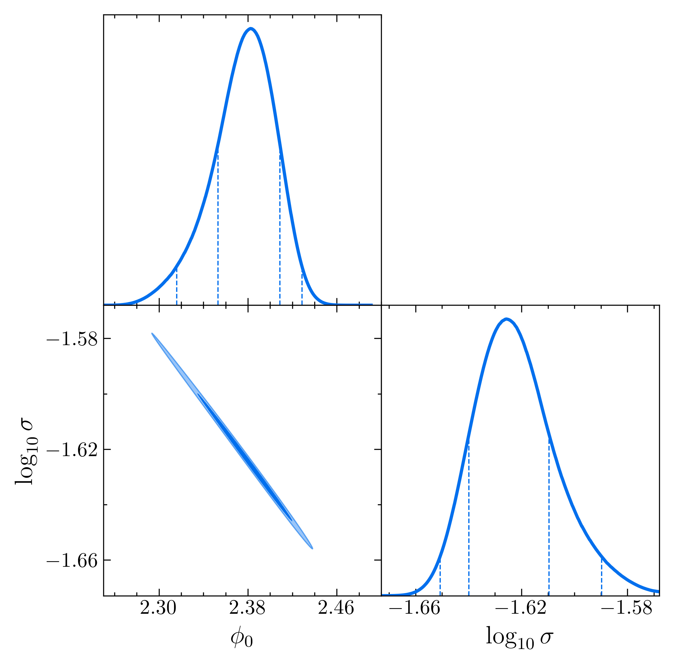
Figure 1: The posterior distributions of the two model parameters $\phi_{0}$ and $\sigma$ (both in the units of $m_{\rm{P}}$). The blue shaded areas correspond to the $68\%$ and $95\%$ CLs. At the $68\%$ CL, we have $\phi_{0}=2.382^{+0.027}_{-0.029}$ and $\log_{10}\sigma=-1.626^{+0.016}_{-0.014}$. It can be clearly seen that $\phi_{0}$ and $\sigma$ exhibit a negative correlation, with strong parameter degeneracy between them.

5.2 Case with three model parameters

Now, we extend our Bayesian analysis by taking the third model parameter $A_{0}$ into account. This means that the plateau on $V_{\rm b}(\phi)$ is allowed to be inclined slightly. The prior distributions of $\phi_{0}$, $\sigma$, and $A_{0}$ can be found in Table 1, and we show our results in Fig. 2. At the $68\%$ CL, we obtain the posterior distributions of $\phi_{0}$ and $\sigma$ as

$$\phi_{0}=2.387^{+0.025}_{-0.027},\quad\log_{10}\sigma=-1.627^{+0.017}_{-0.014}.$$ (19)

These results remain basically the same as those in Eq. (18), but the joint posterior distribution of $\phi_{0}$ and $\sigma$ has become broader compared with Fig. 1, indicating that their parameter degeneracy can be broken to some extent by the introduction of the third parameter $A_{0}$. Moreover, at the $68\%$ CL, we obtain

$$A_{0}=-2.197^{+4.054}_{-0.841}\times 10^{-4}.$$ (20)

The posterior distribution of $A_{0}$ peaks at a relatively small negative value of $A_{0}=-2.197\times 10^{-4}$, suggesting a positive slope of the plateau in the USR region. This result is physically reasonable and can be understood from two aspects. First, if the slope is too positive, the inflaton rolls down its potential too quickly, violating the USR condition. Second, if the slope is too negative, it is very difficult for the inflaton to pass through the USR region. Therefore, we have adopted a narrow prior range for $A_{0}$, in order to avoid the above situations.

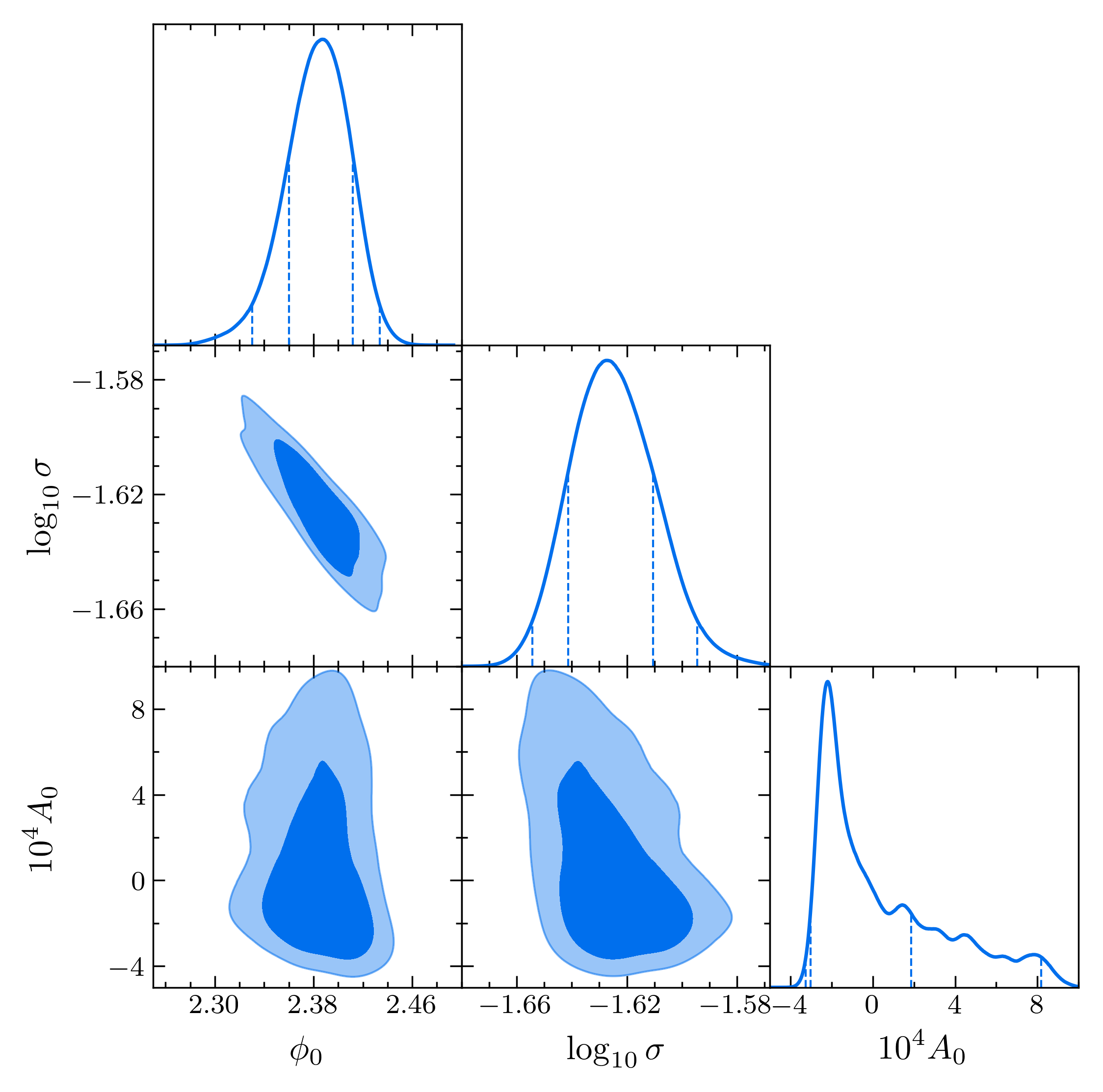
Figure 2: Same as Fig. 1, but with three model parameters $\phi_{0}$, $\sigma$, and $A_{0}$. At the $68\%$ CL, we obtain $\phi_{0}=2.387^{+0.025}_{-0.027}$, $\log_{10}\sigma=-1.627^{+0.017}_{-0.014}$, and $A_{0}=-2.197^{+4.054}_{-0.841}\times 10^{-4}$, respectively. The parameter degeneracy of $\phi_{0}$ and $\sigma$ is somewhat broken by the introduction of $A_{0}$. In addition, $A_{0}$ has high probability with relatively small negative values. This observation prefers the inflation model with a small positively sloped plateau in the USR region.

Till now, we have merely considered the posterior distributions of the model parameters constrained by the NANOGrav 15-year data set. However, these parameters should not only guarantee the GW spectrum, but also must satisfy the constraints on the PBH abundance $f_{\rm PBH}$ at the same time. As a consequence, the parameter spaces in Fig. 2 are still too large. To address this, we calculate $f_{\rm PBH}$ with two different sets of model parameters, both satisfying the posterior distributions in Fig. 2. The first set is $\phi_{0}=2.39$, $\log_{10}\sigma=-1.631$, and $\log_{10}A_{0}=-4.6$, and the second set is $\phi_{0}=2.41$, $\log_{10}\sigma=-1.641$, and $\log_{10}A_{0}=-4.5$, with their comparison illustrated in Fig. 3. We find that the relevant PBH masses are both around $10^{-3}~M_{\odot}$, where the observational constraints mainly come from the lensing experiments Niikura:2019kqi ; Croon:2020wpr . It is obvious that the first set produces reasonable $f_{\rm PBH}$ (the black line), but the second set leads to strong contradiction with the experimental data (the red line). Actually, we will discover that the majority of the parameter spaces in Fig. 2 results in an overproduction of PBHs, so they must be further constrained by $f_{\rm PBH}$.

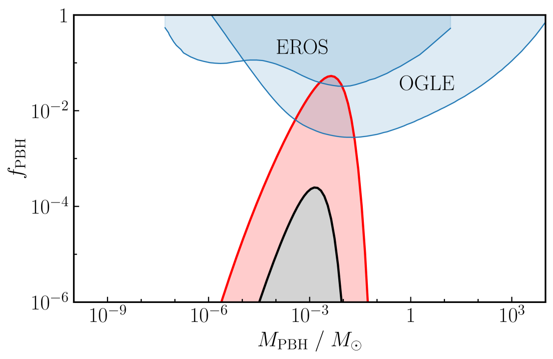
Figure 3: The PBH abundance $f_{\rm PBH}$ obtained with two different sets of model parameters. The black line with $\phi_{0}=2.39$, $\log_{10}\sigma=-1.631$, and $\log_{10}A_{0}=-4.6$ gives reasonable $f_{\rm PBH}$, but the red line with $\phi_{0}=2.41$, $\log_{10}\sigma=-1.641$, and $\log_{10}A_{0}=-4.5$ results in too large $f_{\rm PBH}$, obviously in contradiction with the constraints from Expérience pour la Recherche d’Objets Sombres (EROS) Croon:2020wpr and Optical Gravitational Lensing Experiment (OGLE) Niikura:2019kqi . This observation indicates that the majority of the parameter spaces in Fig. 2 leads to an overproduction of PBHs.

Consequently, it is essential to further constrain the posterior distributions of the model parameters in order to satisfy the PBH abundance. To simplify this analysis, we take $A_{0}$ as various constants: $-2.197\times 10^{-4}$ (the best-fit value) and $\pm 10^{-3}$ (the bounds of its prior distribution), and show the allowed regions in the joint posterior distribution of $\phi_{0}$ and $\sigma$ in Fig. 4. We find that the larger $A_{0}$ is, the smaller the allowed region becomes. This observation indicates the decrease of $\sigma$ with the increase of $A_{0}$ (for the same $\phi_{0}$), meaning that if the USR region has a negative slope, the plateau must be narrow enough, so that the inflaton can roll down its potential definitely.

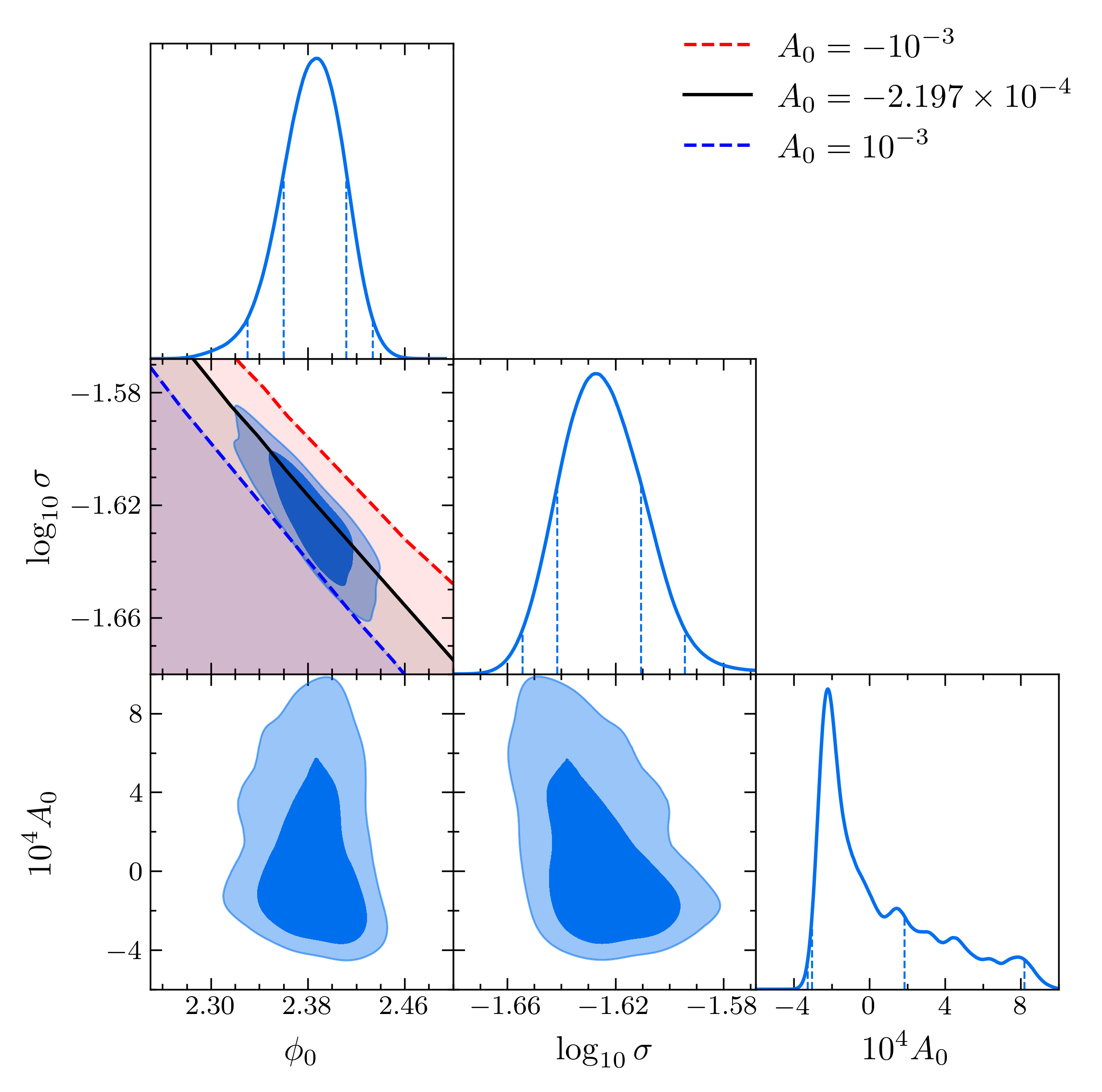
Figure 4: Same as Fig. 2, but with the constraints from the PBH abundance included. We take $A_{0}$ as various constants and plot the allowed regions of $\phi_{0}$ and $\sigma$ in their joint posterior distribution. The overlapped regions with the contours represent the parameter spaces allowed for both the SIGW and PBH constraints (the black line for the best-fit value $A_{0}=-2.197\times 10^{-4}$, and the red and blue dashed lines for $A_{0}=-10^{-3}$ and $10^{-3}$, corresponding to its prior bounds). With the increase of $A_{0}$, the allowed region of $\sigma$ decreases (for the same $\phi_{0}$). This is because, when the slope at $\phi_{0}$ becomes negative, the width of the USR region must be small, otherwise the inflaton cannot roll down its potential. Moreover, the three lines with different $A_{0}$ in the joint posterior distribution of $\phi_{0}$ and $\sigma$ are actually not straight. They seem so only because the prior ranges of $\phi_{0}$ and $\sigma$ are narrow.

Altogether, by means of a modified version of the SIGWfast code Witkowski:2022mtg , the envelope of the SIGW spectrum is plotted in Fig. 5, satisfying the PBH abundance constraint, with $A_{0}=-2.197\times 10^{-4}$ and $\phi_{0}$ and $\sigma$ in the allowed region in their joint posterior disctribution in Fig. 4. For comparison, we also include the sensitivity curves of three next-generation GW detectors: the Square Kilometer Array (SKA) Janssen:2014dka , Laser Interferometer Space Antenna (LISA) LISA:2017pwj , and Big Bang Observer (BBO) Corbin:2005ny . We observe that the SIGW spectrum obtained from our inflation model (the grey belt) not only successfully accounts for the NANOGrav 15-year data set with appropriate amplitude and spectral index, but is also detectable by the GW detectors in future. It should be mentioned that the currently observed signal in the PTA band may limit the sensitivities of the future detectors Babak:2024yhu , but we will not consider it in this work.

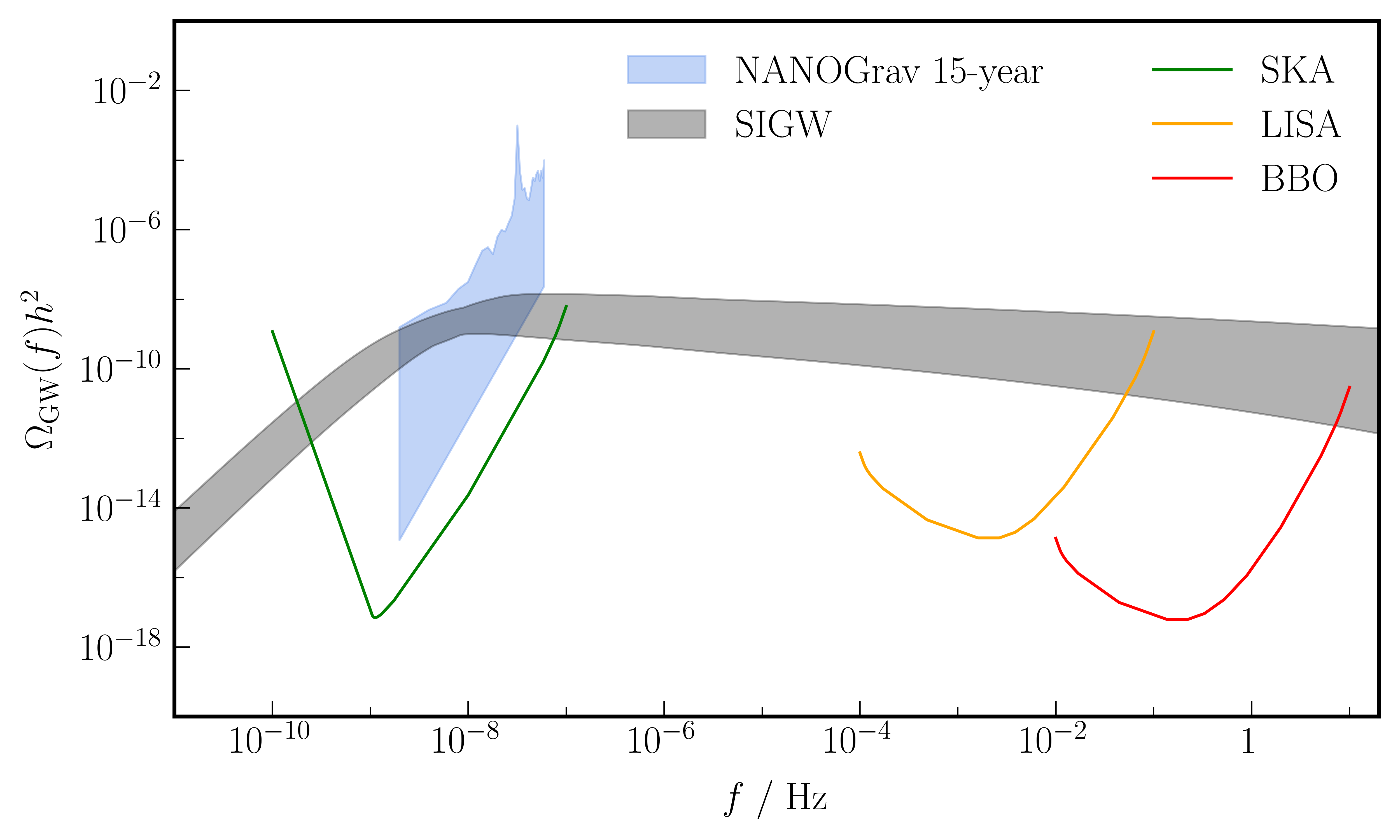
Figure 5: The envelope of the SIGW spectrum $\Omega_{\mathrm{GW}}(f)h^{2}$ (the grey belt) obtained from the model parameters satisfying both the constraints from the NANOGrav 15-year data set and the PBH abundance, with $A_{0}=-2.197\times 10^{-4}$. The light blue shaded region represents the periodogram for the free spectral process from the NANOGrav results, and our SIGW spectrum passes through it with appropriate amplitude and spectral index. In addition, as the SIGW spectrum is already above the sensitivity curves of three next-generation GW detectors: SKA, LISA, and BBO, the SIGWs are expected to be observed in future.

5.3 Case with SMBHBs

Last, we consider the most general case with the impact of SMBHBs. SMBHBs can form during the hierarchical merging process of galaxies in structure formation, and their relevant SGWB lies in the PTA band Rajagopal:1994zj ; Jaffe:2002rt ; Burke-Spolaor:2018bvk . Therefore, we will explore the scenario, in which the SGWB is composed of the SIGWs and the GWs emitted from SMBHBs together, so the total GW spectrum is

$$\Omega_{\mathrm{GW}}=\Omega_{\mathrm{SIGW}}+\Omega_{\mathrm{BHB}}.$$

Now, we face the posterior distributions of five parameters: $\phi_{0}$, $\sigma$, $A_{0}$ (for the inflation model), $A_{\rm BHB}$, and $\gamma_{\rm BHB}$ (for the SMBHBs). Our results are presented in Figs. 6 and 7. At the $68\%$ CL, we have

$$\phi_{0} =2.389_{-0.030}^{+0.026},$$ (21)

$$\log_{10}\sigma =-1.629_{-0.015}^{+0.020},$$ (22)

$$A_{0} =-2.334_{-0.882}^{+9.613}\times 10^{-4},$$ (23)

$$\log_{10}A_{\rm BHB} =-15.646_{-0.557}^{+0.467},$$ (24)

$$\gamma_{\rm BHB} =4.653_{-0.414}^{+0.351}.$$ (25)

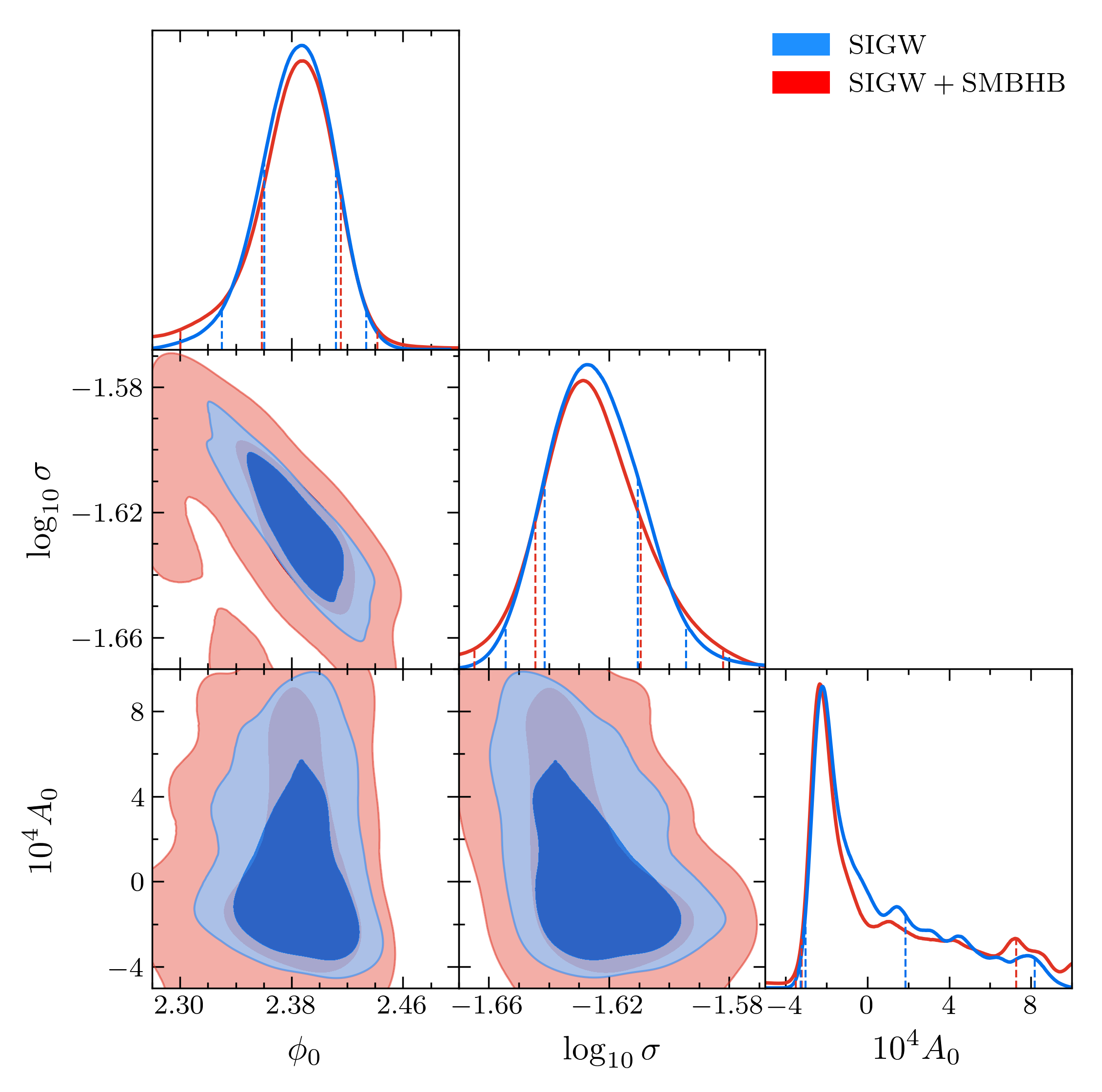
Figure 6: Same as Fig. 2, but with the impact of SMBHBs taken into account. The posterior distributions at the $68\%$ CL read $\phi_{0}=2.389_{-0.030}^{+0.026}$, $\log_{10}\sigma=-1.629_{-0.015}^{+0.020}$, and $A_{0}=-2.334_{-0.882}^{+9.613}\times 10^{-4}$, respectively. We plot the three-parameter SIGW case and the five-parameter $\rm SIGW+SMBHB$ case together for comparison. The joint posterior distributions in the latter are broader. This is because, when only SIGW is considered, the GW spectrum from some parameter combinations is too low to account for the experimental data. However, if the GW spectrum from SMBHBs is large enough, these combinations become allowed again.

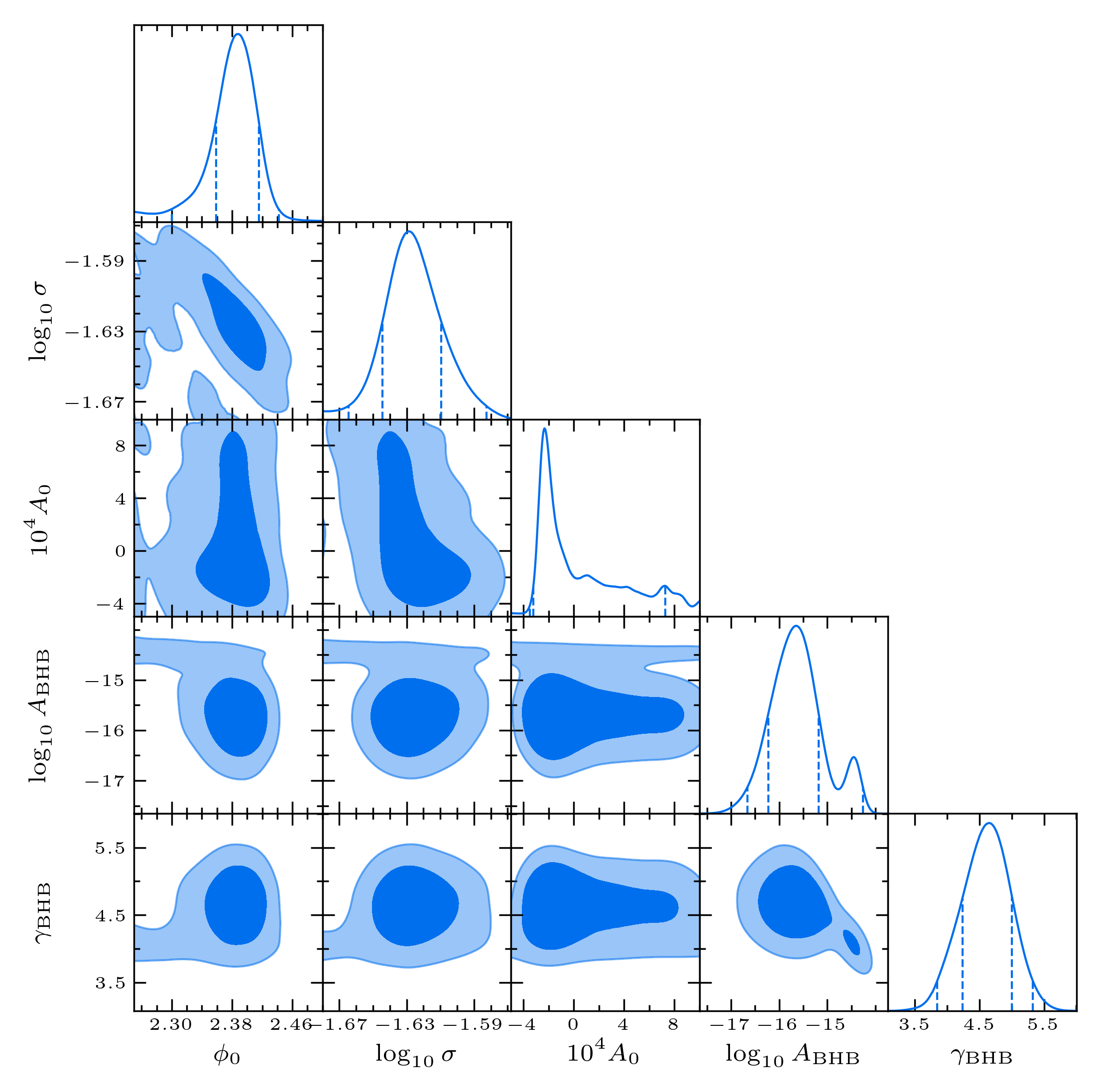
Figure 7: The posterior distributions of the model parameters when the impact of SMBHBs included. There are five model parameters altogether: $\phi_{0}$, $\sigma$, $A_{0}$ (for the inflation model), $A_{\mathrm{BHB}}$, and $\gamma_{\mathrm{BHB}}$ (for the SMBHBs). The posterior distribution of $A_{\rm BHB}$ has two peaks, reflecting the competition between SIGWs and SMBHBs. Different peaks correspond to different components that dominate the GW spectrum, consistent with the analysis by the NANOGrav collaboration in Ref. NANOGrav:2023hvm . The value of the spectral index $\gamma_{\rm BHB}=13/3$ is within its $68\%$ CL when treated as a free parameter.

From Eqs. (21)–(23) and Fig. 6, we observe that all the joint posterior distributions of $\phi_{0}$, $\sigma$, and $A_{0}$ become broader than those in the three-parameter case. This is because, when only SIGW is considered, the GW spectrum from some parameter combinations is too low to match the experimental data. However, as long as the GW spectrum from the SMBHBs is large enough, these parameter combinations again become allowed (e.g., within the $95\%$ CL).

Furthermore, from Fig. 7, we notice that the posterior distribution of $A_{\rm BHB}$ has two peaks, reflecting the competition between SIGWs and SMBHBs. Different peaks correspond to different components that dominate the GW spectrum, consistent with the relevant analysis by the NANOGrav collaboration in Ref. NANOGrav:2023hvm . When $A_{\rm BHB}$ is small, the GW spectrum is dominated by SIGWs; when $A_{\rm BHB}$ is large, the GW spectrum is driven by SMBHBs. Also, the spectral index $\gamma_{\rm BHB}=13/3$ is within the $68\%$ CL when it is treated as a free parameter.

To complete our analysis, we finally calculate the Bayes factors between different models. With the parameters in Eqs. (18)–(25), the Bayes factor between the two-parameter and SMBHB-only models is

$${\cal B}=\frac{{\cal Z}_{\rm SIGW_{2}}}{{\cal Z}_{\rm SMBHB}}=20.21,$$ (26)

the Bayes factor between the three-parameter and SMBHB-only models is

$${\cal B}=\frac{{\cal Z}_{\rm SIGW_{3}}}{{\cal Z}_{\rm SMBHB}}=8.01.$$ (27)

and the Bayes factor between the five-parameter and SMBHB-only models is

$${\cal B}=\frac{{\cal Z}_{\rm SIGW_{3}+SMBHB}}{{\cal Z}_{\rm SMBHB}}=7.36.$$ (28)

The above Bayes factors between different models reveal a clear hierarchy: the two-parameter model $\rm SIGW_{2}$ is strongly favored, followed by the three-parameter model $\rm SIGW_{3}$, with the five-parameter model $\rm SIGW_{3}+SMBHB$ showing the weakest support. However, the fact that the two-parameter model has the largest Bayes factor may be merely caused by fixing $A_{0}=0$ to realize a perfect plateau in the USR region. Since the SIGW spectrum essentially depend on three model parameters, we can only confidently claim that the three-parameter model is slightly better than the five-parameter one, or equivalently, the Bayesian analysis shows no preference with or without SMBHBs. This conclusion is comprehensible, because despite the increase of the number of free model parameters, the complex five-parameter model does not lead to a better fitting to the data. The likelihood does not change much, but meanwhile the prior space expands, so the five-parameter model is not superior to the three-parameter one. Nonetheless, all the two-, three-, and five-parameter models are significantly better than the SMBHB-only model, suggesting that the interpretation of the SGWB from the NANOGrav observations only via the GW spectrum from SMBHBs is not preferred in our inflation model.

6 Conclusion

The exploration on PBHs has aroused increasing interest in physics community in recent years. Besides its possibility as a natural candidate of DM and the source of BHB merger events, another research hotspot is the relevant SIGWs that can be produced with PBHs simultaneously as a second-order effect. Since the detection of the potential SGWB in the PTA band, especially in the NANOGrave 15-year data set, SIGWs have become a promising interpretation in addition to the GWs from SMBHBs. To generate intensive SIGWs with certain amplitudes and frequencies, the usual single-field SR inflation is not enough, and a USR phase is needed, in order to enhance the primordial power spectrum on small scales. The USR phase can be realized by imposing a perturbation on the background inflaton potential, and to determine the position and shape of this perturbation is the purpose of our work.

In this paper, we construct an anti-symmetric perturbation $\delta V(\phi)$ in Eq. (5) with three parameters: $\phi_{0}$, $\sigma$, and $A$ [or equivalently, $A_{0}$ in Eq. (6)], describing the position, width, and slope of $\delta V(\phi)$, and these model parameters further determine the SIGW spectrum. In addition to the SIGWs from the USR inflation, we also consider the GW spectrum from the merger of SMBHBs, which is characterized by another two parameters: the amplitude $A_{\rm BHB}$ and spectral index $\gamma_{\rm BHB}$. Altogether, we encounter a Bayesian analysis with five model parameters, which can be performed via the PTArcade code, with their prior distributions summarized in Table 1.

Our work is composed of three steps. First, in order to reduce computation cost and obtain preliminary results for reference, we directly set the parameter $A_{0}$ to 0, so that the plateau in the USR region is perfect. The posterior distributions of the two parameters $\phi_{0}$ and $\sigma$ can be found in Eqs. (18), and we clearly observe the negative correlation in their joint posterior distribution in Fig. 1, with strong parameter degeneracy.

Then, we set $A_{0}$ as a free parameter, meaning that the plateau in the USR region is allowed to be slightly inclined. In this three-parameter case, the joint posterior distribution of $\phi_{0}$ and $\sigma$ becomes broader, and the posterior distribution of $A_{0}$ peaks at $-2.197\times 10^{-4}$, as can be seen in Fig. 2. This feature indicates that a small positively sloped plateau on the background inflaton potential is preferred. Moreover, we find that some parameter spaces actually overproduce PBHs in certain mass region, as illustrated in Fig. 3. Thus, we further show the allowed parameter regions in Fig. 4, which satisfy both the SIGW and PBH constraints. At last, we plot the SIGW spectrum in Fig. 5, and find that the SIGW spectrum not only accounts for the SGWB, but is also detectable by the next-generation GW detectors.

Finally, we investigate the case with the impact of SMBHBs. We perform the full five-parameter Bayesian analysis, provide their posterior distributions in Figs. 6 and 7, and calculate the Bayes factors between different models in Eqs. (26)–(28). The Bayes factors indicate that the NANOGrav 15-year data set show preference for the two-parameter model, but this may be an artifact of fixing $A_{0}=0$. Hence, we can only confidently claim that the three-parameter model is better than the five-parameter model. However, all the two-, three-, and five-parameter models are significantly favored in Bayesian analysis than the SMBHB-only model.

Altogether, the overall circumstance seems not be improved by increasing the number of free model parameters. Nevertheless, this tendency is consistent with Ref. NANOGrav:2023hvm , in which the NANOGrav collaboration analyzed the Bayes factors between different models with and without SMBHBs, concluding that some models perform better with considering SMBHBs, some are roughly equivalent, while others perform even worse. This primarily depends on whether the increase of model parameters provides a better fitting to the experimental data, and in our present work, it does not yield a substantially better fitting. Therefore, in summary, the simple two-parameter model with a perfect plateau in the USR region has the largest evidence, and is thus favored by the NANOGrav 15-year data set, though it may be just due to the demand that $A_{0}$ vanishes. Moreover, the interpretation of the potential SGWB from the NANOGrav observations via only the GWs generated by SMBHBs is not preferred in our inflation model.

Last, we should mention that we have not discussed the non-Gaussian effects in this work. This includes both the nonlinear relation between the primordial curvature perturbation ${\cal R}$ and the density contrast $\delta$, as well as the intrinsic non-Gaussianity in ${\cal R}$. These non-Gaussianities may lead to notable shifts in the allowed parameter regions and different interpretations of the SGWB, and this will be the topic of our future studies.

- (1) B. P. Abbott et al. [LIGO Scientific and Virgo], Observation of Gravitational Waves from a Binary Black Hole Merger, Phys. Rev. Lett. 116, 061102 (2016), arXiv:1602.03837[gr-qc].
- (2) R. Abbott et al. [KAGRA, VIRGO and LIGO Scientific], GWTC-3: Compact Binary Coalescences Observed by LIGO and Virgo During the Second Part of the Third Observing Run, Phys. Rev. X 13, 041039 (2023), arXiv:2111.03606[gr-qc].
- (3) C. Caprini, M. Hindmarsh, S. Huber, T. Konstandin, J. Kozaczuk, G. Nardini, J. M. No, A. Petiteau, P. Schwaller, G. Servant, and D. J. Weir, Science with the space-based interferometer eLISA. II: Gravitational waves from cosmological phase transitions, J. Cosmol. Astropart. Phys. 04, 001 (2016), arXiv:1512.06239[astro-ph].
- (4) M. Hindmarsh, M. Lüben, J. Lumma, and M. Pauly, Phase transitions in the early universe, SciPost Phys. Lect. Notes 24, 1 (2021), arXiv:2008.09136[astro-ph].
- (5) X. Martin and A. Vilenkin, Gravitational wave background from hybrid topological defects, Phys. Rev. Lett. 77, 2879 (1996), arXiv:9606022[astro-ph].
- (6) D. G. Figueroa, M. Hindmarsh, and J. Urrestilla, Exact Scale-Invariant Background of Gravitational Waves from Cosmic Defects, Phys. Rev. Lett. 110, 101302 (2013), arXiv:1212.5458[astro-ph].
- (7) K. Saikawa, A review of gravitational waves from cosmic domain walls, Universe 3, 40 (2017), arXiv:1703.02576[hep-ph].
- (8) Y. Gouttenoire and E. Vitagliano, Domain wall interpretation of the PTA signal confronting black hole overproduction, Phys. Rev. D 110, L061306 (2024), arXiv:2306.17841[gr-qc].
- (9) D. Baumann, P. Steinhardt, K. Takahash, and K. Ichiki, Gravitational Wave Spectrum Induced by Primordial Scalar Perturbations, Phys. Rev. D 76, 084019 (2007), arXiv:0703290[hep-th].
- (10) E. Bugaev and P. Klimai, Induced gravitational wave background and primordial black holes, Phys. Rev. D 81, 023517 (2010), arXiv:0908.0664[astro-ph].
- (11) J. R. Espinosa, D. Racco, and A. Riotto, A Cosmological Signature of the SM Higgs Instability: Gravitational Waves, JCAP 09, 012 (2018), arXiv:1804.07732[hep-ph].
- (12) K. Kohri and T. Terada, Semianalytic Calculation of Gravitational Wave Spectrum Nonlinearly Induced from Primordial Curvature Perturbations, Phys. Rev. D 97, 123532 (2018), arXiv:1804.08577[gr-qc].
- (13) H. V. Ragavendra, P. Saha, L. Sriramkumar, and J. Silk, Primordial black holes and secondary gravitational waves from ultraslow roll and punctuated inflation, Phys. Rev. D 103, 083510 (2021), arXiv:2008.12202[astro-ph].
- (14) H. V. Ragavendra and L. Sriramkumar, Observational Imprints of Enhanced Scalar Power on Small Scales in Ultra Slow Roll Inflation and Associated Non-Gaussianities, Galaxies 11, 34 (2023), arXiv:2301.08887[astro-ph].
- (15) B. Das, N. Jaman, and M. Sami, Gravitational wave background from quintessential inflation and NANOGrav data, Phys. Rev. D 108, 103510 (2023), arXiv:2307.12913[gr-qc].
- (16) J. Antoniadis et al. [EPTA and InPTA], The second data release from the European Pulsar Timing Array III. Search for gravitational wave signals, Astron. Astrophys. 678, A50 (2023), arXiv:2306.16214[astro-ph].
- (17) A. Zic et al., The Parkes Pulsar Timing Array Third Data Release, Publ. Astron. Soc. Austral. 40, e049 (2023), arXiv:2306.16230[astro-ph].
- (18) H. Xu et al., Searching for the nano-Hertz stochastic gravitational wave background with the Chinese Pulsar Timing Array Data Release I, Res. Astron. Astrophys. 23, 075024 (2023), arXiv:2306.16216[astro-ph].
- (19) G. Agazie et al. [NANOGrav], The NANOGrav 15-year Data Set: Evidence for a Gravitational-Wave Background, Astrophys. J. Lett. 951, L8 (2023), arXiv:2306.16213[astro-ph].
- (20) A. Afzal et al. [NANOGrav], The NANOGrav 15-year Data Set: Search for Signals from New Physics, Astrophys. J. Lett. 951, L11 (2023), arXiv:2306.16219[astro-ph].
- (21) M. T. Miles et al., The MeerKAT Pulsar Timing Array: The 4.5-year data release and the noise and stochastic signals of the millisecond pulsar population, arXiv:2412.01148[astro-ph].
- (22) R. W. Hellings and G. S. Downs, Upper limits on the isotropic gravitational radiation background from pulsar timing analysis, Astrophys. J. Lett. 265, L39 (1983).
- (23) A. Ashoorioon, K. Rezazadeh, and A. Rostami, NANOGrav signal from the end of inflation and the LIGO mass and heavier primordial black holes, Phys. Lett. B 835, 137542 (2022), arXiv:2202.01131[astro-ph].
- (24) G. Franciolini, A. Iovino, Junior, V. Vaskonen, and H. Veermäe, The Recent Gravitational Wave Observation by Pulsar Timing Arrays and Primordial Black Holes: The Importance of Non-Gaussianities, Phys. Rev. Lett. 131, 201401 (2023), arXiv:2306.17149[astro-ph].
- (25) J Ellis, M. Fairbairn, G. Franciolini, G. Hütsi, A. Iovino, M. Lewicki, M. Raidal, J. Urrutia, V. Vaskonen, and H. Veermäe, What is the source of the PTA GW signal?, Phys. Rev. D 109, 023522 (2024), arXiv:2308.08546[astro-ph].
- (26) M. R. Gangopadhyay, V. V. Godithi, R. Inui, K. Ichiki, T. Kajino, A. Manusankar, G. J. Mathews, and Yogesh, Is the NANOGrav detection evidence of resonant particle creation during inflation?, J. High Energy Astrophys. 47, 100358 (2025), arXiv:2309.03101[astro-ph].
- (27) Z. Chang, Y. T. Kuang, D. Wu, and J. Z. Zhou, Probing scalar induced gravitational waves with PTA and LISA: the importance of third order correction, J. Cosmol. Astropart. Phys. 04, 044 (2024), arXiv:2312.14409[astro-ph].
- (28) A. J. Iovino, S. Matarrese, G. Perna, A. Ricciardone, and A. Riotto, How Well Do We Know the Scalar-Induced Gravitational Waves?, arXiv:2412.06764[astro-ph].
- (29) S. Allegrini, L. Del Grosso, A. J. Iovino, and A. Urbano, Is the formation of primordial black holes from single-field inflation compatible with standard cosmology?, arXiv:2412.14049[astro-ph].
- (30) D. Wu, J.-Z. Zhou, Y.-T. Kuang, Z.-C. Li, Z. Chang, and Q.-G. Huang, Can tensor-scalar induced GWs dominate PTA observations?, arXiv:2501.00228[astro-ph].
- (31) Y. Akrami et al. [Planck], Planck 2018 results. X. Constraints on inflation, Astron. Astrophys. 641, A10 (2020), arXiv:1807.06211[astro-ph].
- (32) C. Germani and T. Prokopec, On primordial black holes from an inflection point, Phys. Dark Univ. 18, 6 (2017), arXiv:1706.04226[astro-ph].
- (33) K. Dimopoulos, Ultra slow-roll inflation demystified, Phys. Lett. B 775, 262 (2017), arXiv:1707.05644[hep-ph].
- (34) H. Di and Y. Gong, Primordial black holes and second order gravitational waves from ultra-slow-roll inflation, J. Cosmol. Astropart. Phys. 07, 007 (2018), arXiv:1707.09578[astro-ph].
- (35) A. Ashoorioon, A. Rostami, and J. T. Firouzjaee, Examining the end of inflation with primordial black holes mass distribution and gravitational waves, Phys. Rev. D 103, 123512 (2021), arXiv:2012.02817[astro-ph].
- (36) S. Pi, Y.-l. Zhang, Q.-G. Huang, and M. Sasaki, Scalaron from -gravity as a Heavy Field, J. Cosmol. Astropart. Phys. 05, 042 (2018), arXiv:1712.09896[astro-ph].
- (37) J. Lin, Q. Gao, Y. Gong, Y. Lu, C. Zhang, and F. Zhang, Primordial black holes and secondary gravitational waves from and inflation, Phys. Rev. D 101, 103515 (2020), arXiv:2001.05909[gr-qc].
- (38) S. Saburov and S. V. Ketov, Quantum loop corrections in the modified gravity model of Starobinsky inflation with primordial black hole production, Universe 10, 354 (2024), arXiv:2402.02934[gr-qc].
- (39) L. Wu, Y. Gong, and T. Li, Primordial black holes and secondary gravitational waves from string inspired general no-scale supergravity, Phys. Rev. D 104, 123544 (2021), arXiv:2105.07694[gr-qc].
- (40) R. Ishikawa and S. V. Ketov, Exploring the parameter space of modified supergravity for double inflation and primordial black hole formation, Classical Quantum Gravity 39, 015016 (2022), arXiv:2108.04408[astro-ph].
- (41) R. Ishikawa and S. V. Ketov, Improved model of large-field inflation with primordial black hole production in Starobinsky-like supergravity, Classical Quantum Gravity 41, 195014 (2024), arXiv:2401.11651[astro-ph].
- (42) J. M. Ezquiaga, J. García-Bellido, and E. R. Morales, Primordial Black Hole production in Critical Higgs Inflation, Phys. Lett. B 776, 345 (2018), arXiv:1705.04861[astro-ph].
- (43) M. Cicoli, V. A. Diaz, and F. G. Pedro, Primordial Black Holes from String Inflation, J. Cosmol. Astropart. Phys. 06, 034 (2018), arXiv:1803.02837[hep-th].
- (44) I. Dalianis, A. Kehagias, and G. Tringas, Primordial Black Holes from -attractors, J. Cosmol. Astropart. Phys. 01, 037 (2019), arXiv:1805.09483[astro-ph].
- (45) S.-L. Cheng, W. Lee, and K.-W. Ng, Superhorizon curvature perturbation in ultra-slow-roll inflation, Phys. Rev. D 99, 063524 (2019), arXiv:1811.10108[astro-ph].
- (46) S. S. Mishra and V. Sahni, Primordial Black Holes from a tiny bump/dip in the Inflaton potential, J. Cosmol. Astropart. Phys. 04, 007 (2020), arXiv:1911.00057[gr-qc].
- (47) K. Kefala, G. P. Kodaxis, I. D. Stamou, and N. Tetradis, Features of the inflaton potential and the power spectrum of cosmological perturbations, Phys. Rev. D 104, 023506 (2021), arXiv:2010.12483[astro-ph].
- (48) Y.-P. Wu, E. Pinetti, K. Petraki, and J. Silk, Baryogenesis from ultra-slow-roll inflation, J. High Energy Phys. 01, 015 (2022), arXiv:2109.00118[hep-ph].
- (49) S. Hooshangi, A. Talebian, M. H. Namjoo, and H. Firouzjahi, Multiple Field Ultra Slow Roll Inflation: Primordial Black Holes From Straight Bulk And Distorted Boundary, Phys. Rev. D 105, 083525 (2022), arXiv:2201.07258[astro-ph]
- (50) G. Franciolini and A. Urbano, Primordial black hole dark matter from inflation: the reverse engineering approach, Phys. Rev. D 106, 123519 (2022), arXiv:2207.10056[astro-ph].
- (51) B.-M. Gu, F.-W. Shu, K. Yang, and Y.-P. Zhang, Primordial black holes from an inflationary potential valley, Phys. Rev. D 107, 023519 (2023), arXiv:2207.09968[astro-ph].
- (52) B. Mu, G. Cheng, J. Liu, and Z.-K. Guo, Constraints on ultra-slow-roll inflation from the third LIGO-Virgo observing run, Phys. Rev. D 107, 043528 (2023), arXiv:2211.05386[astro-ph].
- (53) Q. Wang, Y.-C. Liu, B.-Y. Su, and N. Li, Primordial black holes from the perturbations in the inflaton potential in peak theory, Phys. Rev. D 104, 083546 (2021), arXiv:2111.10028[astro-ph].
- (54) Y.-C. Liu, Q. Wang, B.-Y. Su, and N. Li, Primordial black holes from the perturbations in the inflaton potential, Phys. Dark Univ. 34, 100905 (2021).
- (55) J.-X. Zhao, X.-H. Liu, and N. Li, Primordial black holes and scalar-induced gravitational waves from the perturbations on the inflaton potential in peak theory, Phys. Rev. D 107, 043515 (2023), arXiv:2302.06886[astro-ph].
- (56) H.-R. Zhao, Y.-C. Liu, J.-X. Zhao, and N. Li, The evolution of the primordial curvature perturbation in the ultraslow-roll inflation, Eur. Phys. J. C 83, 783 (2023).
- (57) J. X. Zhao and N. Li, An analytical approximation of the evolution of the primordial curvature perturbation in the ultraslow-roll inflation, Eur. Phys. J. C 84, 222 (2024), arXiv:2403.01416[astro-ph].
- (58) B.-Y. Su, N. Li, and L. Feng, Primordial black holes from the ultraslow-roll phase in the inflaton–curvaton mixed field inflation, Eur. Phys. J. C 85, 197 (2025), arXiv:2502.14323[astro-ph].
- (59) L. T. Witkowski, SIGWfast: a python package for the computation of scalar-induced gravitational wave spectra, arXiv:2209.05296[astro-ph]
- (60) E. Thrane and C. Talbot, An introduction to Bayesian inference in gravitational-wave astronomy: parameter estimation, model selection, and hierarchical models, Publ. Astron. Soc. Austral. 36, e010 (2019), arXiv:1809.02293[astro-ph].
- (61) A. Mitridate, D. Wright, R. von Eckardstein, T. Schröder, J. Nay, K. Olum, K. Schmitz, and T. Trickle, PTArcade, arXiv:2306.16377[hep-ph].
- (62) J. E. Gammal et al. [LISA Cosmology Working Group], Reconstructing Primordial Curvature Perturbations via Scalar-Induced Gravitational Waves with LISA, arXiv:2501.11320[astro-ph].
- (63) M. Sasaki, Gauge-Invariant Scalar Perturbations in the New Inflationary Universe, Prog. Theor. Phys. 70, 394 (1983).
- (64) V. F. Mukhanov, Quantum theory of gauge-invariant cosmological perturbations, Sov. Phys. JETP 68, 1297 (1988).
- (65) S. Kachru, R. Kallosh, A. Linde, and S. P. Trivedi, de Sitter Vacua in String Theory, Phys. Rev. D 68, 046005 (2003), arXiv:0301240[hep-th].
- (66) A. M. Green, A. R. Liddle, K. A. Malik, and M. Sasaki, A new calculation of the mass fraction of primordial black holes, Phys. Rev. D 70, 041502 (2004), arXiv:0403181[astro-ph].
- (67) B. J. Carr and S. W. Hawking, Black Holes in the Early Universe, Mon. Not. Roy. Astron. Soc. 168, 399 (1974).
- (68) B. Carr, K. Kohri, Y. Sendouda, and J. Yokoyama, Constraints on Primordial Black Holes, Rept. Prog. Phys. 84, 116902 (2021), arXiv:2002.12778[astro-ph].
- (69) B. J. Carr, The primordial black hole mass spectrum, Astrophys. J. 201, 1 (1975).
- (70) J. M. Bardeen, J. R. Bond, N. Kaiser, and A. S. Szalay, The Statistics of Peaks of Gaussian Random Fields, Astrophys. J. 304, 15 (1986).
- (71) I. Musco, Threshold for primordial black holes: Dependence on the shape of the cosmological perturbations, Phys. Rev. D 100, 123524 (2019), arXiv:1809.02127[gr-qc].
- (72) T. Harada, C. M. Yoo, and K. Kohri, Threshold of primordial black hole formation, Phys. Rev. D 88, 084051 (2013), arXiv:1309.4201[astro-ph].
- (73) A. Escrivà, Simulation of primordial black hole formation using pseudo-spectral methods, Phys. Dark Univ. 27, 100466 (2020), arXiv:1907.13065[gr-qc].
- (74) I. Musco, V. De Luca, G. Franciolini, and A. Riotto, Threshold for primordial black holes. II. A simple analytic prescription, Phys. Rev. D 103, 063538 (2021), arXiv:2011.03014[astro-ph].
- (75) I. Musco and T. Papanikolaou, Primordial black hole formation for an anisotropic perfect fluid: Initial conditions and estimation of the threshold, Phys. Rev. D 106, 083017 (2022), arXiv:2110.05982[gr-qc].
- (76) T. Papanikolaou, Toward the primordial black hole formation threshold in a time-dependent equation-of-state background, Phys. Rev. D 105, 124055 (2022), arXiv:2205.07748[gr-qc].
- (77) I. D. Stamou, Exploring critical overdensity thresholds in inflationary models of primordial black holes formation, Phys. Rev. D 108, 063515 (2023), arXiv:2306.02758[astro-ph].
- (78) G. Domènech, Scalar induced gravitational waves review, Universe 7, 398 (2021), arXiv:2109.01398[gr-qc].
- (79) R. A. Isaacson, Gravitational Radiation in the Limit of High Frequency. I. The Linear Approximation and Geometrical Optics, Phys. Rev. 166, 1263 (1968).
- (80) R. A. Isaacson, Gravitational Radiation in the Limit of High Frequency. II. Nonlinear Terms and the Effective Stress Tensor, Phys. Rev. 166, 1272 (1968).
- (81) K. N. Ananda, C. Clarkson, and D. Wands, The cosmological gravitational wave background from primordial density perturbations, Phys. Rev. D 75, 123518 (2007), arXiv:0612013[gr-qc].
- (82) W.-T. Xu, J. Liu, T.-J. Gao, and Z.-K. Guo, Low-frequency Gravitational Waves from Double-inflection-point Inflation, Phys. Rev. D 101, 023505 (2020), arXiv:1907.05213[astro-ph].
- (83) K. Saikawa and S. Shirai, Precise WIMP Dark Matter Abundance and Standard Model Thermodynamics, J. Cosmol. Astropart. Phys. 08, 011 (2020), arXiv:2005.03544[hep-ph].
- (84) D. Croon, D. McKeen, and N. Raj, Gravitational microlensing by dark matter in extended structures, Phys. Rev. D 101, 083013 (2020), arXiv:2002.08962[astro-ph].
- (85) H. Niikura, M. Takada, S. Yokoyama, T. Sumi, and S. Masaki, Gravitational microlensing by dark matter in extended structures, Phys. Rev. D 99, 083503 (2019), arXiv:1901.07120[astro-ph].
- (86) G. H. Janssen et al., Gravitational wave astronomy with the SKA, Proceedings of Science AASKA14, 037 (2015), arXiv:1501.00127[astro-ph].
- (87) P. Amaro-Seoane et al. [LISA], Laser Interferometer Space Antenna, arXiv:1702.00786[astro-ph].
- (88) V. Corbin and N. J. Cornish, Detecting the Cosmic Gravitational Wave Background with the Big Bang Observer, Classical Quantum Gravity 23, 2435 (2006), arXiv:0512039[gr-qc].
- (89) S. Babak, M. Falxa, G. Franciolini, and M. Pieroni, Forecasting the sensitivity of pulsar timing arrays to gravitational wave backgrounds, Phys. Rev. D 110, 063022 (2024), arXiv:2404.02864[astro-ph].
- (90) M. Rajagopal and R. W. Romani, Ultra-Low Frequency Gravitational Radiation from Massive Black Hole Binaries, Astrophys. J. 446, 543 (1995), arXiv:9412038[astro-ph].
- (91) A. H. Jaffe and D. C. Backer, Gravitational Waves Probe the Coalescence Rate of Massive Black Hole Binaries, Astrophys. J. 583, 616 (2003), arXiv:0210148[astro-ph].
- (92) S. Burke-Spolaor et al., The Astrophysics of Nanohertz Gravitational Waves, Astron. Astrophys. Rev. 27, 5 (2019), arXiv:1811.08826[astro-ph].