Learning Covariance-based Multi-scale Representation of NeuroImaging Measures for Alzheimer Classification

Abstract

Stacking excessive layers in DNN results in highly underdetermined system when training samples are limited, which is very common in medical applications. In this regard, we present a framework capable of deriving an efficient high-dimensional space with reasonable increase in model size. This is done by utilizing a transform (i.e., convolution) that leverages scale-space theory with covariance structure. The overall model trains on this transform together with a downstream classifier (i.e., Fully Connected layer) to capture the optimal multi-scale representation of the original data which corresponds to task-specific components in a dual space. Experiments on neuroimaging measures from Alzheimer’s Disease Neuroimaging Initiative (ADNI) study show that our model performs better and converges faster than conventional models even when the model size is significantly reduced. The trained model is made interpretable using gradient information over the multi-scale transform to delineate personalized AD-specific regions in the brain.

1 Introduction

Literature in the past decades clearly demonstrates that Artificial Neural Network (ANN) has brought significant improvements in various prediction tasks for image data [1, 2]. However, it is also shown that they often require unprecedentedly large amount of data when the ANNs are deeply stacked to learn highly non-linear functions in a data-driven manner [3, 4]. Such an issue limits the use of powerful ANN methods for medical image analyses where sample sizes are limited due to several difficulties in data acquisition [5].

This critical issue is caused from the intrinsic architecture of ANN: the model becomes too flexible and complex even with only a few stacked hidden layers such that relying solely on the large-scale data is inevitable. Therefore, the deeply stacked ANNs, i.e., Deep Learning (DL) approaches, are often used as a black box without much understanding of the behavior mechanism. Several tries [6, 7] have effectively identified on which variables the model cares to come up with a specific decision, e.g., Class Activation Map (CAM) [8] and Grad-CAM [9], but such delineations come from post-hoc analysis of a trained model for a specific target task.

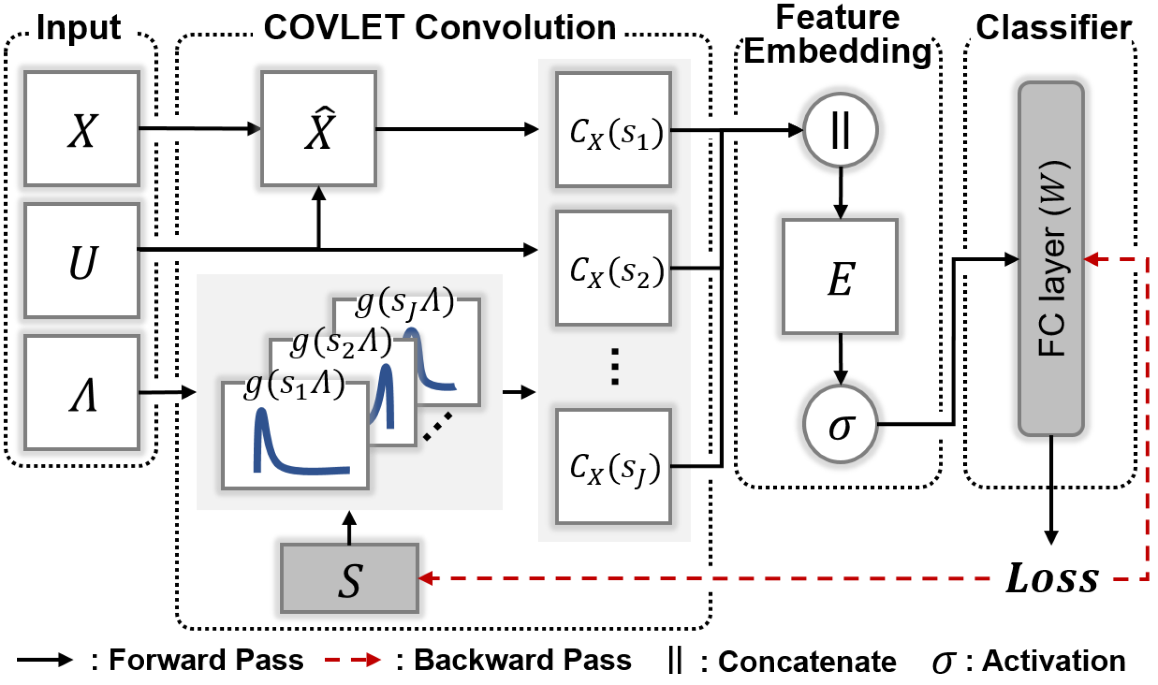
Fig. 1: Overall scheme of our multi-scale learning network. Input $X$ is transformed to a high-dimensional space with kernels $g(s)$ and Principal Components $U$ (i.e., convolution) and fed to a downstream classifier (solid line). The $S$ and classifier are trained to obtain the optimal task-specific multi-scale representation (dashed line).

Essentially, what DL models learn is a transformation of the data into a latent space where the transformed representation is optimized for a target task [10]. Most of the DL approaches learn this transform in a non-parametric data-driven manner that results in estimating exhaustive parameters. In this regime, we propose to utilize parametric kernels (i.e., filter) as in wavelet transform [11], which is formulated as band-pass filtering in the Fourier space (i.e., frequency space). The bottleneck is that typical data (e.g., data matrix) are not defined in time and there is no notion of order of variables, and we tackle this issue using the covariance structure. Leveraging the transform in [12] which defines multi-scale representations using parametric kernels in the space spanned by eigenvectors of a covariance matrix, we design a novel neural network that trains on the “scales” of filters instead of learning the kernel itself. It learns the optimal transform by a simple convolutional filtering, yielding a suitable multi-scale representation for a target task such as classification.

To this end, our work brings the following contributions: 1) we construct a neural network architecture that learns a multi-scale representation of tabular data via its covariance structure, 2) our model is light and trains efficiently even with small number of samples, 3) the proposed model is validated on various imaging measures from Alzheimer’s Disease Neuroimaging Initiative (ADNI) study for classification of diagnostic labels for Alzheimer’s Disease (AD). The experiments on region-wise cortical thickness from magnetic resonance image (MRI) and tau from positron emission tomography (PET) show that our model with a simple convolution layer can distinguish AD-related groups with high precision outperforming conventional ANN with similar architecture.

2 METHODS

As introduced in Fig. 1, we construct an efficient ANN utilizing a transform with parametric kernels summarized by scales and train on the scales only.

2.1 Prelim: Covariance-based Multi-scale Transform

Let $X\in\mathbb{R}^{p\times n}$ be a standardized (zero-mean) feature matrix with $n$ samples with $p$-dimensional feature. Its covariance matrix $\Sigma_{p\times p}=\frac{1}{n}XX^{T}$ shows how each variable is related to each other. Because a covariance matrix is real and symmetric, it has a complete set of orthonormal eigenvectors $U=[u_{1}|u_{2}|...|u_{p}]$ and corresponding positive definite eigenvalues $0<\lambda_{1}\leq...\leq\lambda_{p}$. These eigenvectors, known as Principal Components (PC), define an orthonormal subspace where $X$ can be projected onto with minimal loss of information [13]. Using $U$, $X$ can be transformed as a signal $\hat{X}=U^{T}X$ in a dual space (i.e., an analogue of the frequency space), where an eigenvector that corresponds to a larger eigenvalue captures components of $X$ with high variation. As in conventional frequency analysis, one can apply a filter $g(\cdot)$ on $\hat{X}$ as $g(\Lambda)\hat{X}$ where $\Lambda=diag(\lambda_{1},...,\lambda_{p})$. When the $g(\cdot)$ is a band-pass filter of a specific scale $s$, the formulation becomes a Wavelet-like transform with coefficients

$$\small\vskip-2.0ptC_{X}(s)=Ug(s\Lambda)U^{T}X\vskip-2.0pt$$ (1)

that yields a multi-resolution representation of $X$ on the covariance structure of $\Sigma$. This transform was introduced as Covariance-based Wavelet-like (COVLET) transform in [12].

2.2 Learning Adaptive Kernel with Scales

Given a set of positive and trainable scales $S=[s_{1},s_{2},...,s_{J}]$ where $J=|S|$, each $s_{i}$ yields an embedding of $X$ as $C_{X}(s_{i})=Ug(s_{i}\Lambda)U^{T}X$. With $S\in\mathbb{R}^{J}$ and $X\in\mathbb{R}^{p\times n}$, a set of embeddings is obtained and concatenated together as $E=[C_{X}(s_{1}),C_{X}({s_{2}}),...,C_{X}({s_{J}})]\in\mathbb{R}^{(J\times p)\times n}$ which is a mapping of the $X$ onto a higher-dimensional space. To capture target task-relevant frequency components, the $S$ is trained to minimize a task-specific loss function, e.g., cross-entropy for classification.

If the filter $g(\cdot)$ in (1) is differentiable with respect to $s_{i}$, then the representation from (1) can be optimized according to a task-specific loss $L_{task}$. This is because the derivative $\frac{\partial L_{task}}{\partial s_{i}}$ can be achieved via chain rule as

$$\frac{\partial L_{task}}{\partial s_{i}} =\frac{\partial L_{task}}{\partial C_{X}(s_{i})}\frac{\partial C_{X}(s_{i})}{\partial g(s_{i}\Lambda)}\frac{\partial g(s_{i}\Lambda)}{\partial s_{i}\Lambda}\frac{\partial s_{i}\Lambda}{\partial s_{i}}$$ (2)

$$=\frac{\partial L_{task}}{\partial C_{X}(s_{i})}\frac{\partial C_{X}(s_{i})}{\partial g(s_{i}\Lambda)}g^{\prime}(s_{i}\Lambda)\Lambda.\vskip-2.0pt$$ (3)

Eq. (3) says that the loss can be back-propagated via a gradient descent method throughout the neural network to update $C_{X}(s_{i})$ if $g^{\prime}(\cdot)$ exists. Such optimization achieves the optimal $s_{i}$ that corresponds to a specific scale of the band-pass filter. Learning multi-variate $S$ yields the optimal multi-scale representation $C_{X}(s_{i}),i\in\{1,\cdots,J\}$ of $X$.

To make use of all $C_{X}(s_{i})$ in downstream task, we concatenated these multi-scale representations into $E$. Because $E$ is a linear transform of $X$, an activation function $\sigma$ is required to make our network non-linear toward $X$ as $\sigma(E)$. We feed this non-linear multi-scale representation $\sigma(E)$ to classifier (i.e., fully connected layer with weights $W$) at the end, which produces a class-wise prediction $\hat{y}$. The overall architecture trains on $W$ and $S$ to minimize multi-class cross-entropy between the $\hat{y}$ and the ground truth $y$.

Model Interpretation. When a sample is fed to a trained model, with a back-propagation of the model’s prediction (i.e. class label), gradients are computed toward every layer’s input. Considering each gradient as an importance measure of corresponding input in the layer, weighted combination with layer’s input followed by Rectified Linear Unit (ReLU) tells us which variable is related to the model’s prediction, and this is known as Grad-CAM [9]. In our framework, Grad-CAM can be obtained for every multi-scaled representation $C_{X}(s_{i})$. To figure out the ROI-wise influence across the scales, the Grad-CAM is averaged across the scale to yield a measure $M$ for $k$-th input variable on $c$-th class as

$$\small\vskip-3.0ptM^{c}(k)=\sum_{i=1}^{J}ReLU(\frac{\partial\hat{y}_{c}}{\partial C_{X_{k}}(s_{i})}\cdot C_{X_{k}}(s_{i}))\vskip-1.0pt$$ (4)

where $\hat{y}_{c}$ is a class-wise prediction and $C_{X_{k}}(s_{i})$ denotes embedding of $k$-th input variable with $s_{i}$. The $M$ identifies ROI-wise effect of a specific label for each subject.

3 EXPERIMENTAL RESULTS

In this section, we perform two experiments on ADNI data to validate the performance and efficiency of our method.

Table 1: Demographics of ADNI dataset

Biomarker	Category	CN	EMCI	LMCI	AD
Cortical Thickness	# of Subjects	844	490	250	240
	Age (mean, std)	74.1$\pm$8.1	71.3$\pm$7.5	72.0$\pm$7.7	74.1$\pm$8.1
	Gender (M/F)	490/354	282/208	148/102	149/91
Tau protein	# of Subjects	237	186	105	85
	Age (mean, std)	72.0$\pm$5.9	70.1$\pm$7.0	70.6$\pm$7.7	72.6$\pm$8.0
	Gender (M/F)	119/118	110/76	61/44	43/42

Table 2: Performance comparison of baselines and our model (with 16 scales) on each two classification tasks from two different biomarkers. The number of parameters in each model is reported together (except Linear SVM).

Biomarker	Methods	CN vs. EMCI				CN vs. EMCI vs. LMCI vs. AD
		# Params	Accuracy	Recall	Precision	# Params	Accuracy	Recall	Precision
Cortical Thickness	Linear SVM	-	0.738$\pm$0.026	0.734$\pm$0.031	0.725$\pm$0.027	-	0.742$\pm$0.017	0.726$\pm$0.022	0.739$\pm$0.027
	1-MLP	0.3K	0.738$\pm$0.023	0.728$\pm$0.034	0.723$\pm$0.027	0.6K	0.683$\pm$0.014	0.655$\pm$0.018	0.669$\pm$0.013
	2-MLPR	5.2K	0.759$\pm$0.019	0.754$\pm$0.029	0.745$\pm$0.021	10.5K	0.692$\pm$0.011	0.672$\pm$0.012	0.679$\pm$0.017
	2-MLPI	25.9K	0.765$\pm$0.045	0.759$\pm$0.053	0.750$\pm$0.048	26.2K	0.702$\pm$0.013	0.681$\pm$0.010	0.691$\pm$0.016
	Ours $(J$$=$$16)$	5.1K	0.858$\pm$0.029	0.849$\pm$0.036	0.846$\pm$0.030	10.2K	0.800$\pm$0.021	0.788$\pm$0.035	0.785$\pm$0.030
Tau Protein	Linear SVM	-	0.615$\pm$0.015	0.593$\pm$0.017	0.613$\pm$0.023	-	0.515$\pm$0.029	0.458$\pm$0.033	0.575$\pm$0.052
	1-MLP	0.3K	0.608$\pm$0.032	0.589$\pm$0.034	0.600$\pm$0.036	0.6K	0.504$\pm$0.020	0.479$\pm$0.027	0.519$\pm$0.035
	2-MLPR	5.2K	0.648$\pm$0.030	0.635$\pm$0.033	0.642$\pm$0.034	10.5K	0.540$\pm$0.019	0.514$\pm$0.020	0.563$\pm$0.047
	2-MLPI	25.9K	0.653$\pm$0.032	0.642$\pm$0.036	0.648$\pm$0.035	26.2K	0.556$\pm$0.012	0.521$\pm$0.016	0.590$\pm$0.018
	Ours $(J$$=$$16)$	5.1K	0.726$\pm$0.060	0.721$\pm$0.064	0.723$\pm$0.063	10.2K	0.577$\pm$0.016	0.553$\pm$0.016	0.585$\pm$0.046

3.1 ADNI Dataset

For the experiments, we used MRI and PET imaging measures from the public ADNI study. The images were registered to Destrieux atlas [14] to obtain region-wise measures from 148 cortical regions and 12 sub-cortical regions, i.e., total of 160 regions. Grey matter biomarkers (i.e., cortical thickness from 148 cortical regions and grey matter volume from 12 sub-cortical regions) were derived from the MRI, and tau measure was obtained from the PET scans. The dataset consists of 4 AD-specific progressive groups: Cognitively Normal (CN), Early Mild Cognitive Impairment (EMCI), Late Mild Cognitive Impairment (LMCI) and Alzheimer’s Disease (AD). The demographics of ADNI dataset is summarized in Table 1.

3.2 Experiment Setup

Group Comparisons. In our experiment, we designed tasks of 2-way (CN vs. EMCI) and 4-way (CN vs. EMCI vs. LMCI vs. AD) classifications to validate qualitative and quantitative performances of the proposed method.

Baselines. We adopted four baseline methods: 1) Linear Support Vector Machine (Linear SVM), 2) Multi-Layer Perceptron with one layer (1-MLP) and 3,4) with two layers (2-MLP_I, 2-MLP_R). For the 2-MLP, we tried two cases where the number of hidden nodes were consistent as the input dimension (2-MLP_I) or reduced to have similar number of parameters with our methods when $J$$=$$16$ (2-MLP_R).

Evaluation. For unbiased and fair comparison, we carefully tuned baseline methods and used 5-fold cross validation (CV) in every experiment. For evaluation, we used mean accuracy, precision and recall across the CV. Precision and recall were averaged with equal importance for each class.

Training. Due to the imbalance in class labels, we oversampled training dataset using ADASYN [15]. For our method, we tried various number of kernels $J\in[2,64]$, with each scale initialized uniformly between [0.1,10] in $\log_{10}$-space. Performance analysis on the $J$ is given in Section 3.5. Network weights were randomly initialized with He initialization [16] and trained with AdamW [17] optimizer including both classifier $W$ and scale parameters $S$. Learning rates for $W$ and $S$ were set separately within $[0.001,0.03]$, but their effects were marginal. To prevent overfitting, weight decay at 0.01 was adopted for every linear layer. Spline kernel in [18] was used for $g(\cdot)$ as it behaves as a smooth band-pass filter.

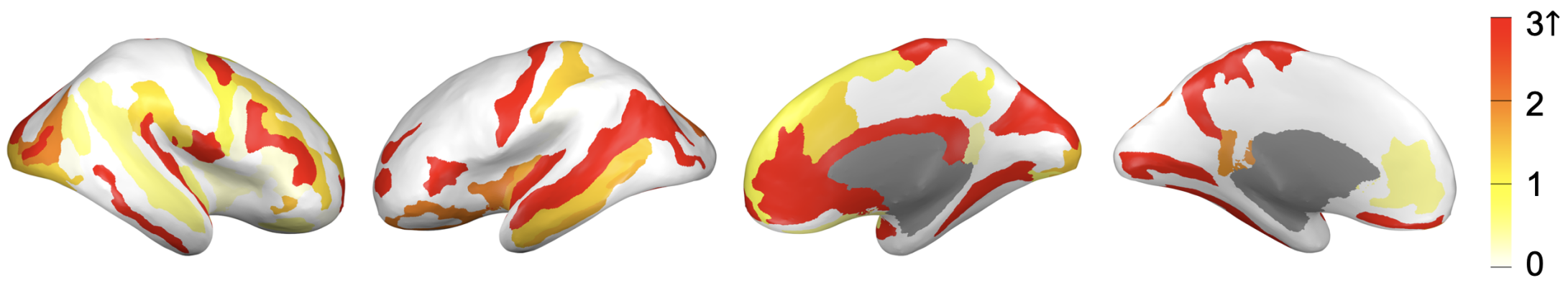
Fig. 2: Visualization of $M$ on a random AD-sample that identifies personalized AD-specific ROIs. Various AD-specific ROIs are identified as in [19, 20, 21] including hippocampus, thalamus, amygdala and several temporal regions. Drawings were generated using BrainPainter [22].

3.3 Performance Evaluation

Our model is evaluated on two classification tasks as in Section 3.2 to demonstrate that it can classify different AD-related classes. For every experiment, we reported performances in mean and standard deviation from 5-fold CV and they are summarized in Table 2. In every experiment, stacking one more layer on 1-MLP, i.e., 2-MLP_R and 2-MLP_I, increased the performance where that of 2-MLP_I was better than 2-MLP_R possibly due to larger model size. On top of the MLPs, our model with $J$$=$$16$ outperformed them with less or similar model sizes.

3.3.1 2-way Classification: CN vs. EMCI

We first demonstrate the performance of our model together with baselines on a binary classification task where CN and EMCI groups are distinguished. This is not an easy problem as the variation caused by AD in the preclinical stage is subtle.

Cortical Thickness. Linear SVM and single layer classifier (1-MLP) achieved almost 74% in accuracy. Stacking one more linear layer (2-MLP_R, 2-MLP_I), accuracy increased only $\sim$2% even though model size increased drastically. However, when the convolution layer of our method with $J$$=$$16$ was added to the 1-MLP, it gained $\sim$12% in accuracy even with significantly less number parameters than 2-MLP_I. Compared to 2-MLP_R with comparable model size, our model with $J$$=$$16$ outperformed by $\sim$10% in accuracy.

Tau Protein. We observed similar accuracy patterns in Tau as in the cortical thickness analysis. While 2-layered classifiers (2-MLP_R, 2-MLP_I) achieved nearly 4% increase in accuracy compared to single layer classifier, our model with $J$$=$$16$ even outperformed 2-layered classifiers by 7%.

3.3.2 4-way Classification: CN vs. EMCI vs. LMCI vs. AD

We extend the experiment to validate our model with a more difficult case. Here, the expected accuracy with a random guess is only 25% and guessing with the majority class (i.e., CN) is $46.8\%$ for cortical thickness and $38.7\%$ for tau.

Cortical Thickness. Classifier with MLPs (1-MLP, 2-MLP_R, 2-MLP_I) achieved $\sim$70% in accuracy even worse than Linear SVM which reached 74% in accuracy. Even in this complicated task, our model with $J$$=$$16$ yielded $80\%$ in accuracy surpassing other 2-MLP baselines over 10% with less number of parameters. Precision and recall were around $0.78$ demonstrating that the model worked reasonably well.

Tau Protein. Linear SVM and 1-MLP achieved only about 50% in accuracy. While 2-MLP_R and 2-MLP_I outperformed 1-MLP in the accuracy by 4 to 5%, Ours ($J$$=$$16$) surpassed them. Overall performances were not as good as in cortical thickness. This may be because tau measures vary in the early stages of AD [23], which may not be a suitable biomarker to characterize later stages of MCI and AD.

3.4 Interpretation from Trained Model

In Fig. 2, we visualize Grad-CAM result using Eq. (4) from Section 2.2. This result was derived by inputting cortical thickness from a randomly selected AD sample into our pre-trained model with 4-way classification setting. It delineates which ROIs the model considered importantly to classify it as an AD sample, which include superior temporal, hippocampus, thalamus, amygdala and many others which are very well-known to be AD-specific in other literature [19, 20, 21].

3.5 Discussions on Model Behavior

Convergence. In Table 2, our proposed model has less number of parameters than stacking another linear layer as in 2-MLP_I. To show fast convergence of our model, we compared the convergence between ours and 2-MLP_I with the same objective function. The test accuracy on 4-way (CN vs. EMCI vs. LMCI vs. AD) classification with 5-fold CV is shown in Fig. 3 using the same learning rate set for both models.

As shown in Fig. 3, with same learning rates of 0.1 or 0.01, our proposed model converged faster than 2-MLP_I. To reach the test accuracy of 0.6, our model required 110 and 50 epochs for 0.01 and 0.1 respectively. However, 2-MLP_I with learning rate of 0.01 required 430 epochs and cannot even reach when learning rate was 0.1 showing unstable pattern across 5 folds with very high variations.

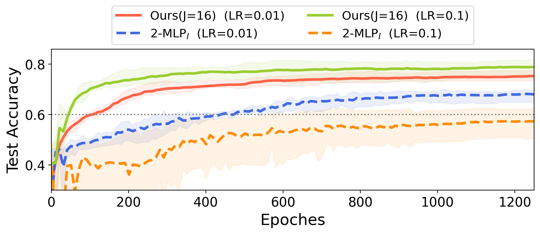
Fig. 3: Comparisons of mean test accuracy from our model and 2-MLP_I on 4-way classification with cortical thickness. Our model reaches 0.6 significantly faster than 2-MLP_I. Measures are computed from 5-fold CV (shaded areas are range of the test accuracy).

Effect of Number of Scales. In Section 2.2, we hypothesized that each kernel is capable of capturing important frequency components. To capture various task-specific components with kernels, we need sufficient number of scales. Fig. 4 shows the test accuracy with respect to the number of scales. For each experiment, hyperparameters were tuned to obtain the best results. The test accuracy kept increasing with respect to the number of scales until $J$$=$$16$ for both cortical thickness and tau. After $J$$=$$16$, the performance remained the same or degraded. This may be because the data are being mapped to too high-dimensional space with the increase of $J$.

Effect of Training on Scale. To show that training on the scales improves the model performance, we compared the results of training the same model with and without training on $S$. As shown in Fig. 4, the classification results on both biomarkers improved with the training of scales. However, as more scales were adopted, effect of training on scales decreased. This may be because the COVLET transform in many scales sufficiently captures all the necessary components for classifying AD-specific groups from the beginning. One may argue that simply adopting more scales can replace the training of scales, but such an approach will significantly increase the dimension of a latent space (i.e., curse of dimensionality) and the number of model parameters.

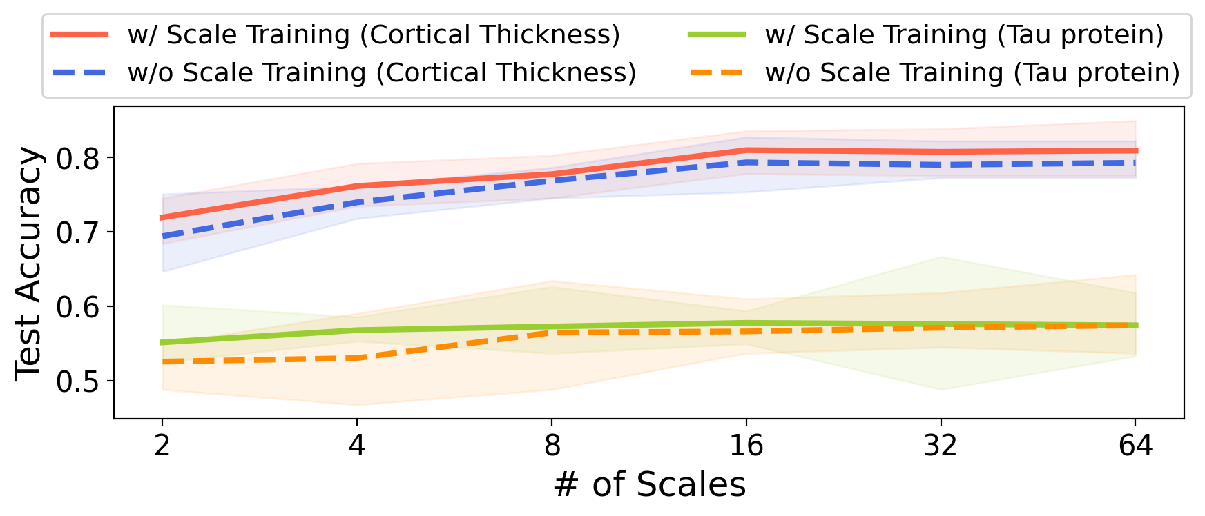
Fig. 4: Mean test accuracy w.r.t. scale in our model on 4-way classification using cortical thickness (5-fold CV). Test accuracy improves with scale training (solid line) over without training (dashed line).

4 CONCLUSION

We proposed an efficiently trainable framework with small sample-sized datasets by utilizing trainable parametric kernels and sample covariance structure. The kernels are defined as band-pass filters in a dual space spanned by eigenvectors of the covariance matrix, whose scales are trained with a task-specific loss. The training process achieves multi-scale representation that captures task-specific components in the dual space. Our model is validated on classifications of diagnostic labels of AD (and preclinical AD) for performance and convergence, and identifies personalized AD-relevant ROIs supported by other literature.

5 Acknowledgement

This research was supported by HU22C0168, IITP-2022-2020-001461 (ITRC), HU22C0171, NIH R03 AG070701 and NRF-2022R1A2C2092336 and IITP-2019-0-01906 (AI Graduate Program at POSTECH).

References

- [1] Shervin Minaee, Yuri Boykov, et al., “Image segmentation using deep learning: A survey,” IEEE TPAMI, vol. 44, no. 7, pp. 3523–3542, 2022.
- [2] Geert Litjens, Thijs Kooi, et al., “A survey on deep learning in medical image analysis,” Medical image analysis, vol. 42, pp. 60–88, 2017.
- [3] Frank Emmert-Streib et al., “An introductory review of deep learning for prediction models with big data,” Frontiers in Artificial Intelligence, vol. 3, pp. 4, 2020.
- [4] Muhammad Imran Razzak et al., “Deep learning for medical image processing: Overview, challenges and the future,” Classification in BioApps, pp. 323–350, 2018.
- [5] Dinggang Shen, Guorong Wu, and Heung-Il Suk, “Deep learning in medical image analysis,” Annual review of biomedical engineering, vol. 19, pp. 221, 2017.
- [6] Amina Adadi and Mohammed Berrada, “Peeking inside the black-box: a survey on explainable artificial intelligence (xai),” IEEE access, vol. 6, pp. 52138–52160, 2018.
- [7] Riccardo Guidotti, Anna Monreale, Salvatore Ruggieri, et al., “A survey of methods for explaining black box models,” ACM computing surveys (CSUR), vol. 51, no. 5, pp. 1–42, 2018.
- [8] Bolei Zhou, Aditya Khosla, Agata Lapedriza, Aude Oliva, and Antonio Torralba, “Learning deep features for discriminative localization,” in CVPR, 2016, pp. 2921–2929.
- [9] Ramprasaath R Selvaraju, Michael Cogswell, et al., “Grad-cam: Visual explanations from deep networks via gradient-based localization,” in ICCV, 2017, pp. 618–626.
- [10] Fan Yang, Rui Meng, Hyuna Cho, et al., “Disentangled sequential graph autoencoder for preclinical alzheimer’s disease characterizations from adni study,” in MICCAI. Springer, 2021, pp. 362–372.
- [11] S.G. Mallat, “A theory for multiresolution signal decomposition: the wavelet representation,” TPAMI, vol. 11, no. 7, pp. 674–693, 1989.
- [12] Fan Yang, Amal Isaiah, and Won Hwa Kim, “Covlet: covariance-based wavelet-like transform for statistical analysis of brain characteristics in children,” in MICCAI. Springer, 2020, pp. 83–93.
- [13] Hervé Abdi and Lynne J Williams, “Principal component analysis,” Wiley interdisciplinary reviews: computational statistics, vol. 2, no. 4, pp. 433–459, 2010.
- [14] Christophe Destrieux, Bruce Fischl, Anders Dale, et al., “Automatic parcellation of human cortical gyri and sulci using standard anatomical nomenclature,” Neuroimage, vol. 53, no. 1, pp. 1–15, 2010.
- [15] Haibo He, Yang Bai, Edwardo A. Garcia, and Shutao Li, “Adasyn: Adaptive synthetic sampling approach for imbalanced learning,” in IJCNN, 2008, pp. 1322–1328.
- [16] Kaiming He, Xiangyu Zhang, Shaoqing Ren, and Jian Sun, “Delving deep into rectifiers: Surpassing human-level performance on imagenet classification,” in ICCV, 2015, pp. 1026–1034.
- [17] Ilya Loshchilov and Frank Hutter, “Decoupled weight decay regularization,” ICLR, 2019.
- [18] David K Hammond, Pierre Vandergheynst, and Rémi Gribonval, “Wavelets on graphs via spectral graph theory,” Applied and Computational Harmonic Analysis, vol. 30, no. 2, pp. 129–150, 2011.
- [19] Huanqing Yang, Xu, et al., “Study of brain morphology change in alzheimer’s disease and amnestic mild cognitive impairment compared with normal controls,” General psychiatry, vol. 32, no. 2, 2019.
- [20] Pruessner Jens C Lerch, Jason P et al., “Focal decline of cortical thickness in alzheimer’s disease identified by computational neuroanatomy,” Cerebral cortex, vol. 15, no. 7, pp. 995–1001, 2005.
- [21] Jason P Lerch, Jens Pruessner, Zijdenbos, et al., “Automated cortical thickness measurements from mri can accurately separate alzheimer’s patients from normal elderly controls,” Neurobiology of aging, vol. 29, no. 1, pp. 23–30, 2008.
- [22] Răzvan V Marinescu, Arman Eshaghi, et al., “Brainpainter: A software for the visualisation of brain structures, biomarkers and associated pathological processes,” in Multimodal Brain Image Analysis and Mathematical Foundations of Computational Anatomy, pp. 112–120. Springer, 2019.
- [23] Clifford R Jack Jr, Knopman, et al., “Hypothetical model of dynamic biomarkers of the alzheimer’s pathological cascade,” The Lancet Neurology, vol. 9, no. 1, pp. 119–128, 2010.