On the convexity for the range set of two quadratic functions

Abstract

Given $n\times n$ symmetric matrices $A$ and $B,$ Dines in 1941 proved that the joint range set $\{(x^{T}Ax,x^{T}Bx)|~x\in\mathbb{R}^{n}\}$ is always convex. Our paper is concerned with non-homogeneous extension of the Dines theorem for the range set $\mathbf{R}(f,g)=\{\left(f(x),g(x)\right)|~x\in\mathbb{R}^{n}\},$ $f(x)=x^{T}Ax+2a^{T}x+a_{0}$ and $g(x)=x^{T}Bx+2b^{T}x+b_{0}.$ We show that $\mathbf{R}(f,g)$ is convex if, and only if, any pair of level sets, $\{x\in\mathbb{R}^{n}|f(x)=\alpha\}$ and $\{x\in\mathbb{R}^{n}|g(x)=\beta\}$, do not separate each other. With the novel geometric concept about separation, we provide a polynomial-time procedure to practically check whether a given $\mathbf{R}(f,g)$ is convex or not.

1 Introduction

Given a pair of quadratic functions, $f(x)=x^{T}Ax+2a^{T}x+a_{0}$ and $g(x)=x^{T}Bx+2b^{T}x+b_{0}$, where $A,~B$ are $n\times n$ real symmetric matrices, $a,b\in\mathbb{R}^{n}$ and $a_{0},b_{0}\in\mathbb{R},$ their joint numerical range, a subset of $\mathbb{R}^{2},$ is defined to be

$$\mathbf{R}(f,g)=\left\{(f(x),g(x))~|~x\in\mathbb{R}^{n}\right\}\subset\mathbb{R}^{2}.$$

In this paper, we are interested in the fundamental mathematical problem:

$$\text{(P)}:\text{ When, and only when, the joint range }\mathbf{R}(f,g)\text{ is convex?}$$

The first result regarding (P) was an original paper by Dines [2, 1941]. He showed that the joint range of two homogeneous quadratic forms $\left\{(x^{T}Ax,x^{T}Bx)~|~x\in\mathbb{R}^{n}\right\}$ is always convex. Though a special case of (P), Yakubovich [15, 1971] used it to prove the classical $\mathcal{S}$-lemma, which later became an indispensable tool in optimization and the control theory. The $\mathcal{S}$-lemma asserts that, if $g(x)\leq 0$ satisfies Slater’s condition, namely, there is an $\overline{x}\in\mathbb{R}^{n}$ such that $g(\overline{x})<0$, the following two statements are equivalent:

• (${\rm S_{1}}$)   ($\forall x\in\mathbb{R}^{n}$) $~g(x)\leq 0~\Longrightarrow~f(x)\geq 0.$

• (${\rm S_{2}}$)   $(\exists\mu\geq 0)$  $f(x)+\mu g(x)\geq 0,~\forall x\in\mathbb{R}^{n}.$

A number of interesting applications follow from the $\mathcal{S}$-lemma. In particular, it can be used to show a highly non-trivial result that quadratic program with one quadratic inequality constraint

$$({\rm QP1QC})~~~~~\inf_{x\in\mathbb{R}^{n}}\left\{f(x)~|~g(x)\leq 0\right\}$$

always adopts strong duality, while $f$ and $g$ are not necessarily convex. Survey and extensions of the $\mathcal{S}$-lemma are referred to, for example, Derinkuyu and Pinar [3, 2006], Pólik and Terlaky [10, 2007], Tuy and Tuan [12, 2013], Xia et al. [13, 2016].

The convexity of the joint numerical range $\mathbf{R}(f,g)$ also allows to reformulate and solve difficult optimization problems. Nguyen et al. [6, 2020] proposed to solve the following special type of quadratic optimization problem with a joint numerical range constraint:

$$({\rm Po4})\quad\begin{array}[]{cl}\displaystyle\inf_{(x,z)\in\mathbb{R}^{n}\times\mathbb{R}^{2}}&F(z)\\ \text{ s.t. }&\alpha z_{1}+\beta z_{2}-\gamma\leq 0\\ &z=\left(z_{1},z_{2}\right)\in\mathbf{R}(f,g)\end{array}$$

where $\alpha,\beta,\gamma\in\mathbb{R}^{m}$ and $F(z_{1},z_{2})$ is a convex quadratic function from $\mathbb{R}^{2}$ to $\mathbb{R}$. They showed that, if the joint range set $\mathbf{R}(f,g)$ is convex, (Po4) has an equivalent SDP reformulation. Then, some important optimization problems in the literature can be solved, including

• (Not solved efficiently before) Ye and Zhang [16, 2003] proposed to minimize the absolute value of a quadratic function over a quadratic constraint:

  $$({\rm AQP})\quad\begin{array}[]{cl}\displaystyle\inf_{x\in\mathbb{R}^{n}}&\left|x^{T}Ax+2a^{T}x+a_{0}\right|\\ \text{ s.t. }&x^{T}Bx+2b^{T}x+b_{0}\leq 0.\end{array}$$

  It was suggested in [16, 2003] to solve the problem $({\rm AQP})$, under strict conditions, by the bisection method, each iteration of which requires to do an SDP. In [6, 2020], by the help of the convexity of $\mathbf{R}(f,g),$ the problem $({\rm AQP})$ can be resolved completely without any condition.

• (Not solved before) The quadratic hypersurface intersection problem proposed by Pólik and Terlaky [10, 2007]: given two quadratic surfaces $f(x)=0$ and $g(x)=0$, how to determine whether the two quadratic surfaces $f(x)=0$ and $g(x)=0$ has intersection without actually computing the intersection? The problem can be reformulated as the following non-linear least square problems:

  $$({\rm QSIC})\quad\begin{array}[]{cl}\displaystyle\inf_{\left(x^{T},z_{1},z_{2}\right)^{T}\in\mathbb{R}^{n+2}}&\left(z_{1}\right)^{2}+\left(z_{2}\right)^{2}\\ \text{ s.t. }&\left\{\begin{array}[]{l}f(x)-z_{1}=0\\ g(x)-z_{2}=0,\end{array}\right.\end{array}$$

  which is a type of $({\rm Po4}).$ In [6, 2020], Nguyen et al. showed that, if $\mathbf{R}(f,g)$ is convex, $({\rm QSIC})$ can be solved by an SDP. If not, it can be solved directly by elementary analysis.

• (Not solved efficiently before) The double well potential problems (DWP) in [5, 14, 2017]:

  $$\begin{array}[]{rl}({\rm DWP})&\displaystyle\inf_{x\in\mathbb{R}^{n}}~\frac{1}{2}\left(\frac{1}{2}\|Px-p\|^{2}-r\right)^{2}+\frac{1}{2}x^{T}Qx-q^{T}x\end{array},$$

  where $Q$ is an $n\times n$ symmetric matrix, $P\neq 0$ is an $m\times n$ matrix, $p\in\mathbb{R}^{m},r\in\mathbb{R}$, and $q\in\mathbb{R}^{n}$. The original development for solving (DWP) used elementary (but lengthy) approach. By identifying (DWP) as a special type of (Po4), it can now be solved with just an SDP.

Though the characterization of the convexity of $\mathbf{R}(f,g)$ is a useful tool for solving optimization problems, in literature, progresses from Dines’ result to the convexity of $\mathbf{R}(f,g)$ for general $f(x)=x^{T}Ax+2a^{T}x+a_{0}$ and $g(x)=x^{T}Bx+2b^{T}x+b_{0}$ have been very slow. The Dines theorem becomes invalid when either $f$ or $g$ or both adopt linear terms. Here is an example with configurations for easy understanding.

Example 1.

Let $f(x,y)=-x^{2}+y^{2}$ and $g(x)=-2x^{2}+2y^{2}+4x-2y$ where $g(x)$ has linear terms. In this example,

$$A=\left[\begin{array}[]{r r}-1&0\\ 0&1\end{array}\right]~\text{ and }~B=\left[\begin{array}[]{r r}-2&0\\ 0&2\end{array}\right].$$

Fig. 1a shows that $\left\{(x^{T}Ax,x^{T}Bx)~|~x\in\mathbb{R}^{n}\right\}$ is a straight line and hence convex. Fig. 1b gives the graph of $\mathbf{R}(f,g)$, which is apparently non-convex.

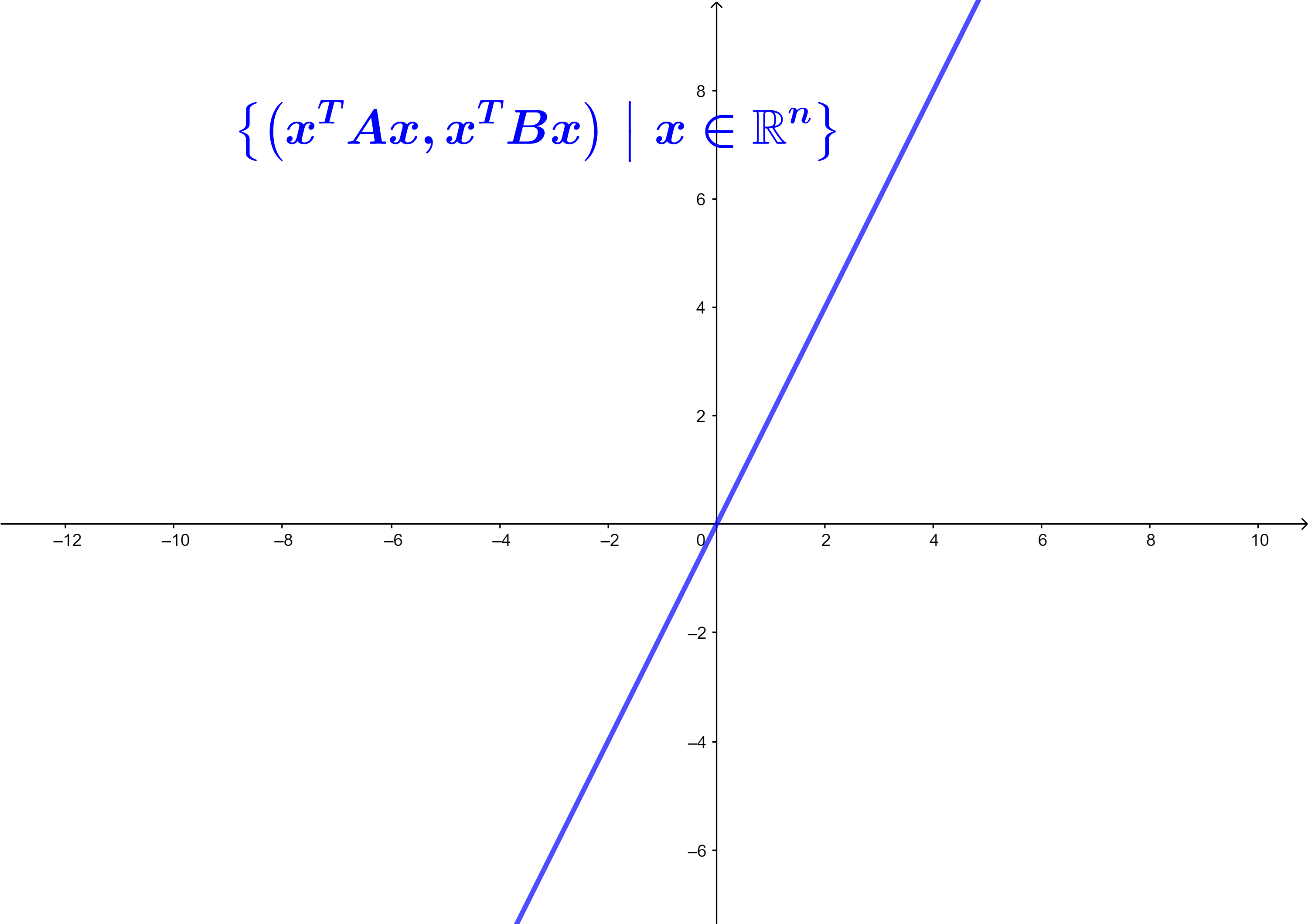
a The set $\left\{(x^{T}Ax,x^{T}Bx)~|~x\in\mathbb{R}^{n}\right\}$ in Example 1 is a straight line.

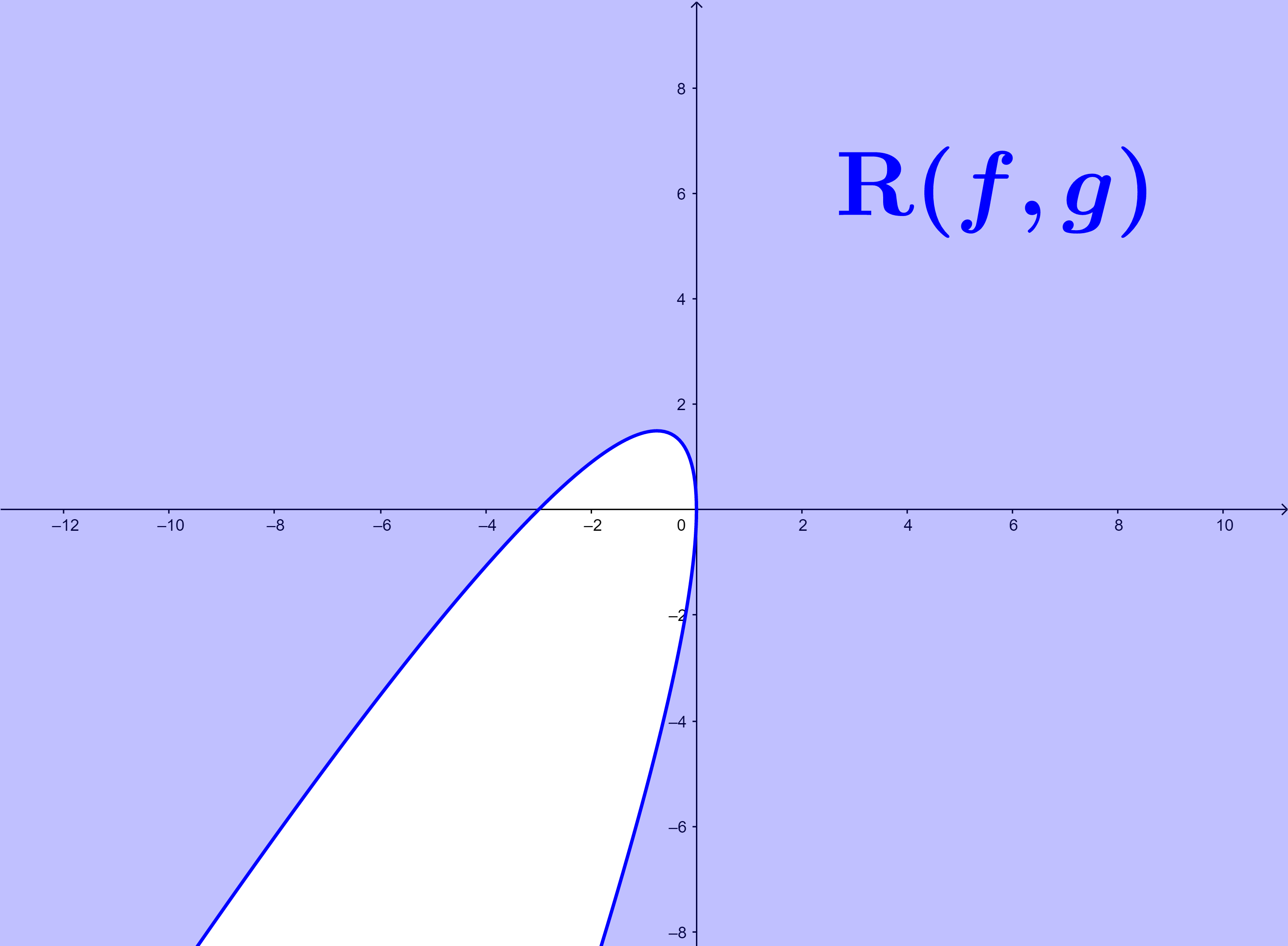
b The shaded region is the joint range $\mathbf{R}(f,g)$ in Example 1.

Figure 1: The graph corresponds to Example 1.

For a long period of time, the best generalization of the Dines theorem has been Polyak’s sufficient condition [9, 1998] (The fourth row in Table 1). It was not until 2016 that Flores-Bazán and Opazo [4, 2016] (last row in Table 1) completely characterized the convexity of $\mathbf{R}(f,g)$ with a set of necessary and sufficient conditions. Over a period of 75 years from 1941 to 2016, notable results related to (P) include, in chronological order, Brickmen [1, 1961], an unpublished manuscript by Ramana and Goldman [11, 1995], and Polyak [9, 1998]. Among them, we feel that Brickmen’s [1, 1961] and Flores-Bazán and Opazo’s [4, 2016] results are the most fundamental. They are summarized in Table 1.

1941 (Dines [2])	(Dines Theorem) $\left\{\left.\left(x^{T}Ax,x^{T}Bx\right)~\right|~x\in\mathbb{R}^{n}\right\}$ is convex. Moreover, if $x^{T}Ax$ and $x^{T}Bx$ has no common zero except for $x=0$, then $\left\{\left.\left(x^{T}Ax,x^{T}Bx\right)~\right|~x\in\mathbb{R}^{n}\right\}$ is either $\mathbb{R}^{2}$ or an angular sector of angle less than $\pi$.
1961 (Brickmen [1])	$\mathbf{K}_{A,B}=\left\{\left.\left(x^{T}Ax,x^{T}Bx\right)~\right|~x\in\mathbb{R}^{n}~,~\|x\|=1\right\}$ is convex if $n\geq 3$.
1995 (Ramana & Goldman [11]) Unpublished	$\mathbf{R}(f,g)=\left\{\left.\left(f(x),g(x)\right)~\right|~x\in\mathbb{R}^{n}\right\}$ is convex if and only if $\mathbf{R}(f,g)=\mathbf{R}(f_{H},g_{H})+\mathbf{R}(f,g)$, where $f_{H}(x)=x^{T}Ax$ and $g_{H}(x)=x^{T}Bx$.
	$\mathbf{R}(f,g)=\left\{\left.\left(f(x),g(x)\right)~\right|~x\in\mathbb{R}^{n}\right\}$ is convex if $n\geq 2$ and $\exists~\alpha,\beta\in\mathbb{R}$ such that $\alpha A+\beta B\succ 0$.
1998 (Polyak [9])	$\left\{\left.\left(x^{T}Ax,x^{T}Bx,x^{T}Cx\right)~\right|~x\in\mathbb{R}^{n}\right\}$ is convex if $n\geq 3$ and $\exists~\alpha,\beta,\gamma\in\mathbb{R}$ such that $\alpha A+\beta B+\gamma C\succ 0$.
	$\left\{\left.\left(x^{T}A_{1}x,\cdots,x^{T}A_{m}x\right)~\right|~x\in\mathbb{R}^{n}\right\}$ is convex if $A_{1},\cdots,A_{m}$ commute.
2016 (Bazán & Opazo [4])	$\mathbf{R}(f,g)=\left\{\left.\left(f(x),g(x)\right)~\right|~x\in\mathbb{R}^{n}\right\}$ is convex if and only if $\exists~d=(d_{1},d_{2})\in\mathbb{R}^{2}$, $d\neq 0$, such that the following four conditions hold: (C1) $F_{L}\left(\mathcal{N}(A)\cap\mathcal{N}(B)\right)=\{0\}$ (C2) $d_{2}A=d_{1}B$ (C3) $-d\in\mathbf{R}(f_{H},g_{H})$ (C4) $F_{H}(u)=-d\implies\left\langle F_{L}(u),d_{\perp}\right\rangle\neq 0$ where $\mathcal{N}(A)$ and $\mathcal{N}(B)$ denote the null space of $A$ and $B$ respectively, $F_{H}(x)=\left(f_{H}(x),g_{H}(x)\right)=\left(x^{T}Ax,x^{T}Bx\right)$, $F_{L}(x)=\left(a^{T}x,b^{T}x\right)$, and $d_{\perp}=(-d_{2},d_{1})$.

Table 1: Chronological list of notable results related to problem (P)

Flores-Bazán and Opazo’s result [4, 2016] (last row in Table 1) is considered fundamental by us because they were the first to provide a complete answer to problem (P). Their results rely heavily on an unpublished manuscript by Ramana and Goldman [11, 1995] (third row in Table 1). In [11, 1995], it was shown that $\mathbf{R}(f,g)$ is convex if and only if the following relation holds:

$$\mathbf{R}(f,g)=\mathbf{R}(f_{H},g_{H})+\mathbf{R}(f,g),$$ (1)

where $f_{H}(x)=x^{T}Ax,~g_{H}(x)=x^{T}Bx.$ For example, let $f(x,y,z)=x^{2}+y^{2}$ and $g(x,y,z)=-x^{2}+y^{2}+z.$ Figure 2a shows that $\mathbf{R}(f,g)$ is the right half-plane, while Figure 2b is the joint range of the homogeneous part $\mathbf{R}(f_{H},g_{H})$ which is an angular sector of angle $\pi/2$. In this example, it can be checked that

$$\mathbf{R}(f_{H},g_{H})+\mathbf{R}(f,g)=\bigcup_{y\in\mathbf{R}(f,g)}\mathbf{R}(f_{H},g_{H})+y\subset\mathbf{R}(f,g).$$

Moreover, there is $\mathbf{R}(f,g)\subset\mathbf{R}(f_{H},g_{H})+\mathbf{R}(f,g),$ which verifies (1) for this example.

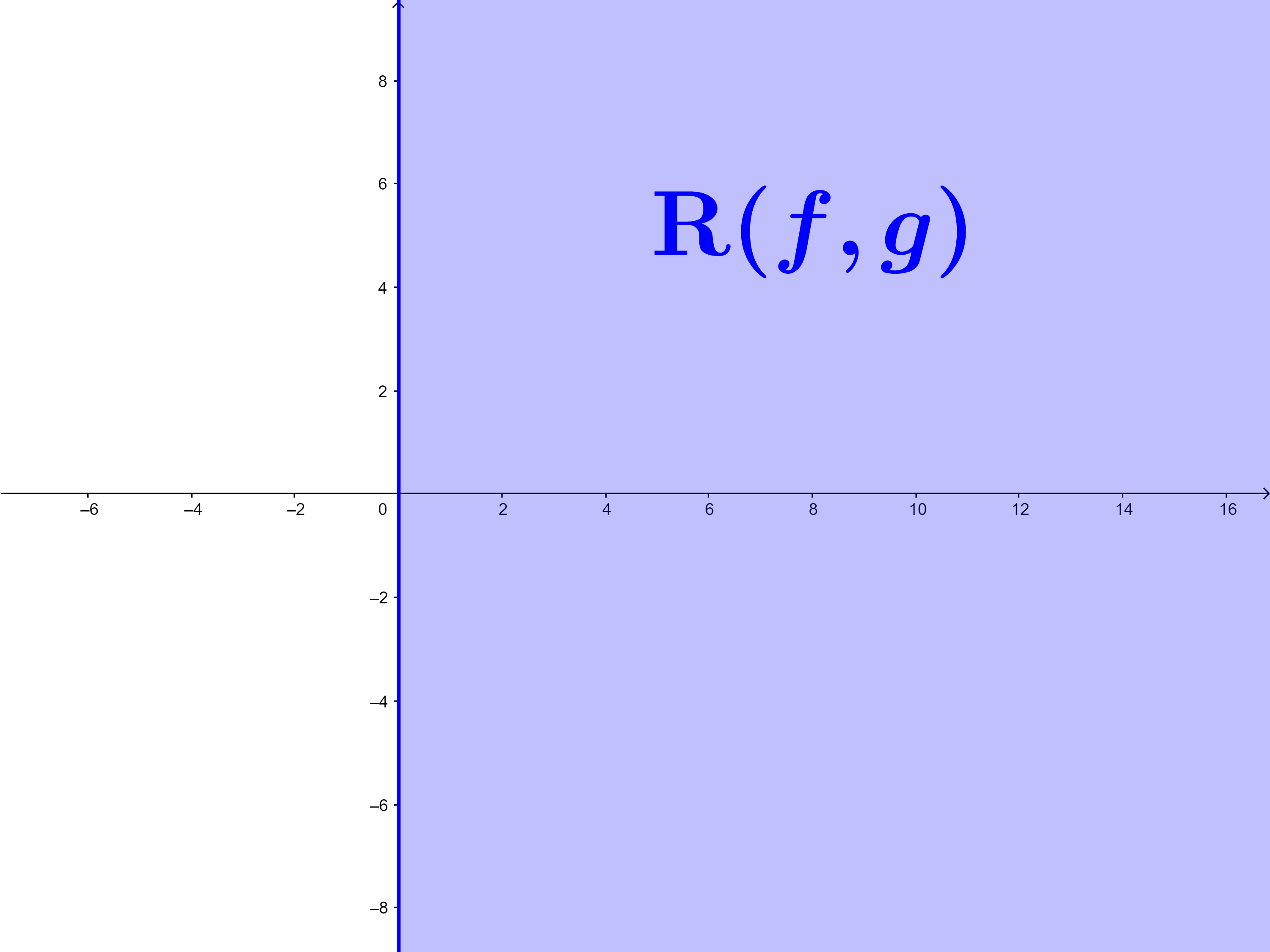
a The joint range $\mathbf{R}(f,g)$ is the right half-plane.

b The joint range of the homogeneous part $\mathbf{R}(f_{H},g_{H})$ is an angular sector of angle $\pi/2$.

Figure 2: Let $f(x,y,z)=x^{2}+y^{2}$ and $g(x,y,z)=-x^{2}+y^{2}+z$.

Characterizing necessary and sufficient conditions for (P) from (1) is technical and tedious. Flores-Bazán and Opazo [4, 2016] wrote a 34-pages long paper to complete it. Moreover, they do not describe how more difficult the convexity can be tackled efficiently, i.e., how does one determine whether there exists an appropriate $d=(d_{1},d_{2})\in\mathbb{R}^{2}$, $d\neq 0$ such that the conditions (C1)-(C4) (last row in Table 1) are satisfied?

The main purpose of this paper is to provide a different view and thus a different set of necessary and sufficient conditions to describe problem (P) with fully geometric insights. We indeed borrow the tools from Nguyen and Sheu [7, 2019] in which a new concept called “separation of quadratic level sets” was introduced. The idea was first used to give a neat proof for the $\mathcal{S}$-lemma with equality by Xia et al. [13, 2016]. We show in this paper that the same idea can be extended to accommodate our purpose to check the convexity of $\mathbf{R}(f,g)$ by a constructive polynomial-time procedure.

The paper is developed in the following sequence.

• In Section 2, we shall review the concept of separation of two sets and list several properties for separation of two quadratic level sets.

• In Section 3, we obtain the main result “the joint numerical range $\mathbf{R}(f,g)$ is non-convex if and only if there exists $\alpha,\beta\in\mathbb{R}$ such that $\{x\in\mathbb{R}^{n}|~g(x)=\beta\}$ separates $\{x\in\mathbb{R}^{n}|~f(x)=\alpha\}$ or $\{x\in\mathbb{R}^{n}|~f(x)=\alpha\}$ separates $\{x\in\mathbb{R}^{n}|~g(x)=\beta\}$.

• In Section 4, a polynomial-time procedure for checking the convexity of $\mathbf{R}(f,g)$ is provided.

• In Section 5, we prove that the result of Flores-Bazán and Opazo [4, 2016] is an implication of our result in Section 3.

• Finally, we conclude our paper by briefly mentioning the relation between the convexity of joint range $\mathbf{R}(f,g)$ and variants of $\mathcal{S}$-lemma.

Throughout the paper, we adopt the following notations. For a matrix $P$, the symbol $P^{\dagger}$ denotes the Moore-Penrose generalized inverse of $P$. The null space and range space of $P$ is denoted by $\mathcal{N}(P)$ and $\mathcal{R}(P)$ respectively. For a subspace $W$ of $\mathbb{R}^{n}$, $W^{\perp}$ denotes the orthogonal complement of $W$ with respect to the standard inner product equipped on $\mathbb{R}^{n}$. For conciseness, given a real constant $\alpha$, the set $\{f=\alpha\}\triangleq\{x\in\mathbb{R}^{n}|~f(x)=\alpha\}$ is called the $\alpha$-level set of $f$, and $\{f<\alpha\}\triangleq\{x\in\mathbb{R}^{n}|~f(x)<\alpha\}$ is said to be the $\alpha$-sublevel set of $f$.

2 Separation of Quadratic Level Sets

Given a pair of quadratic functions $f$ and $g,$ Nguyen and Sheu in [7, 2019] introduced the following definition for “separation of level sets”:

Definition 1 ([7]).

The $0$-level set $\{g=0\}$ is said to separate the set $\{f\star 0\}$, where $\star\in\{<,=\}$, if there are non-empty subsets $L^{-}$ and $L^{+}$ of $\{f\star 0\}$ such that

$$L^{-}\cup L^{+}=\{f\star 0\}~\text{ and }$$ (2)

$$g(u^{-})g(u^{+})<0,~\forall~u^{-}\in L^{-};~\forall~u^{+}\in L^{+}.$$

Several remarks directly from the definition should be noted.

1. When $\{g=0\}$ separates $\{f\star 0\}$, $\{f\star 0\}$ must be disconnected. Otherwise, by the Intermediate Value Theorem, $g(\{f\star 0\})$ is a connected interval containing the point $0,$ which contradicts to Definition 1.

2. An affine set of the type $\{f\star 0\}$ with $\star\in\{<,=\}$ cannot be separated by any other $\{g=0\}.$ This is due to $\{f\star 0\}$ for $\star\in\{<,=\}$ being always connected, provided that $f$ is affine.

3. $\{g=0\}$ separates $\{f<0\}$ $\centernot\Longrightarrow$ $\{g=0\}$ separates $\{f=0\}.$ Figure 4 shows such an example.

4. $\{g=0\}$ separates $\{f=0\}$ $\centernot\Longrightarrow$ $\{g=0\}$ separates $\{f<0\}.$ See Figure 4.

5. $\{g=0\}$ separates $\{f=0\}$ $\centernot\Longrightarrow$ $\{f=0\}$ separates $\{g=0\}.$ A simple example is that $g$ is affine. A hyperplane $\{g=0\}$ can easily separate the other supersurface $\{f=0\},$ but it may not be separated reversely. See Figure 4.

6. $\{g=0\}$ separates $\{f=0\}$ $\centernot\Longrightarrow$ $\{g=\alpha\}$ separates $\{f=\beta\}$ for $\alpha,~\beta\in\mathbb{R}.$ That is, for separation property, the “hight” associated with the contour matters. See Figure 5.

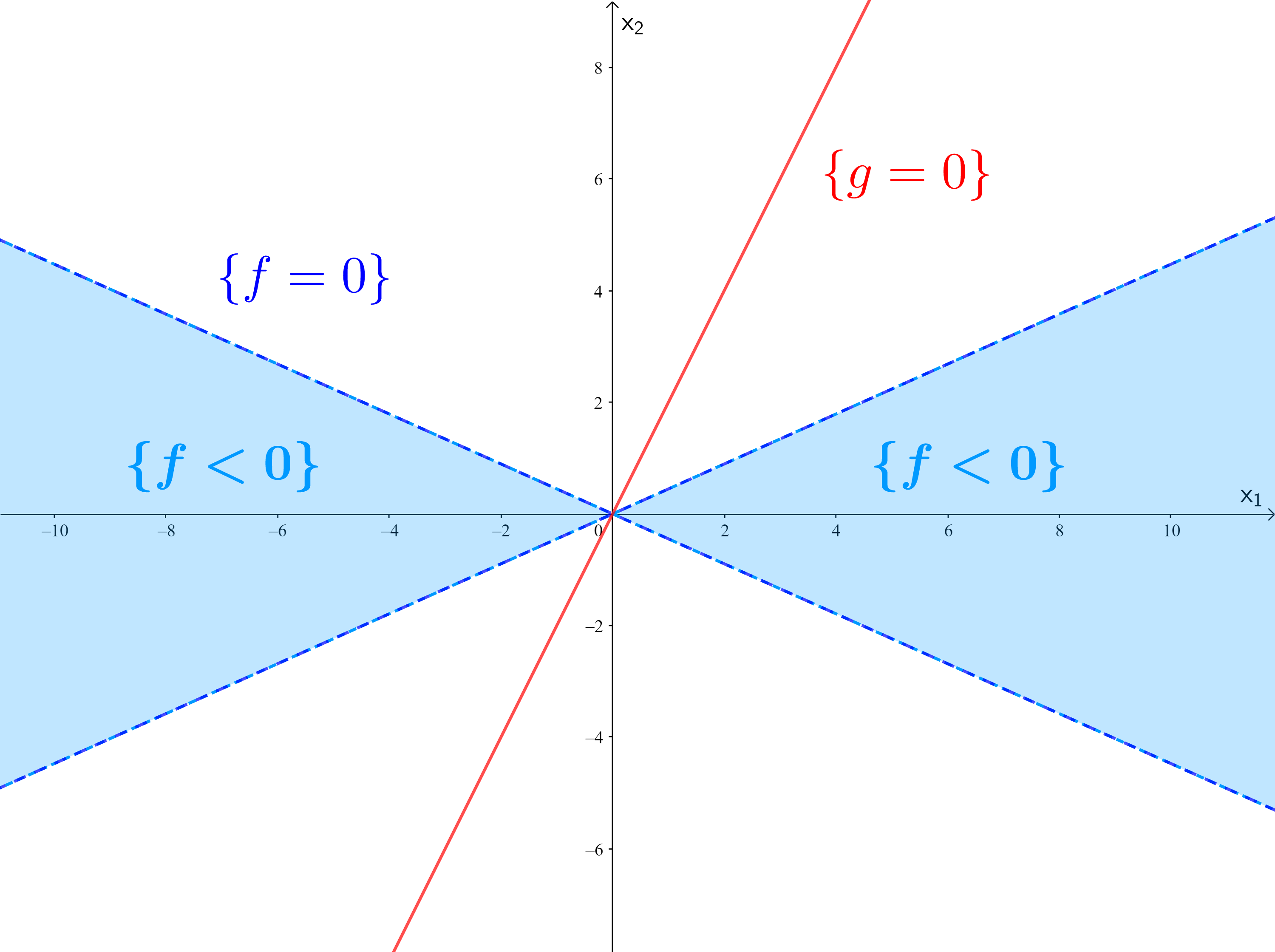
Figure 3: For remark (c) and remark (e). Let $f(x,y)=-x^{2}+4y^{2}$ and $g(x,y)=2x-y$. The level set $\{g=0\}$ separates $\{f<0\},$ while $\{g=0\}$ does not separate $\{f=0\}.$

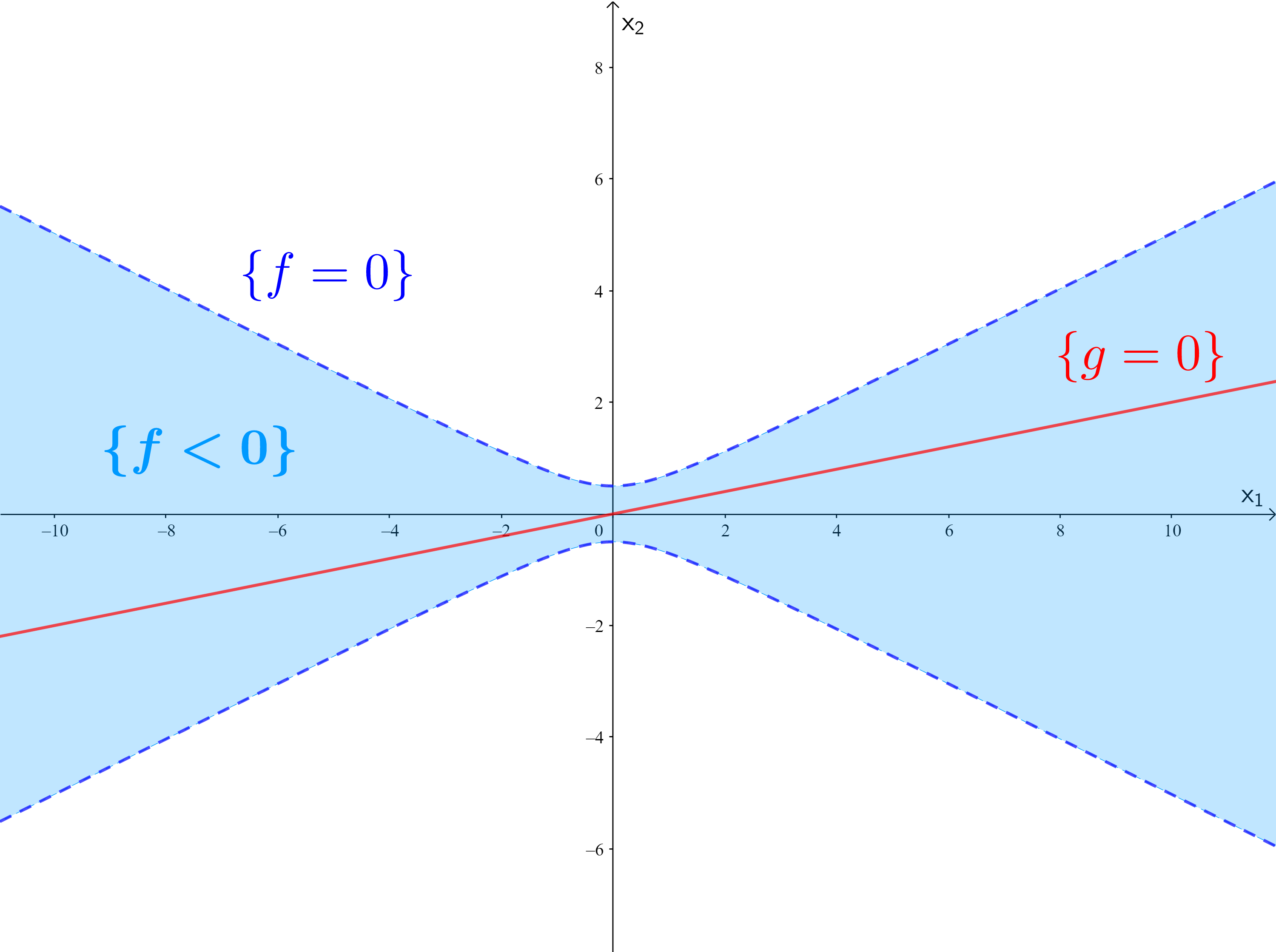
Figure 4: For remark (d). Let $f(x,y)=-x^{2}+4y^{2}-1$ and $g(x,y)=x-5y$. The level set $\{g=0\}$ separates $\{f=0\}$ while $\{g=0\}$ does not separate $\{f<0\}.$

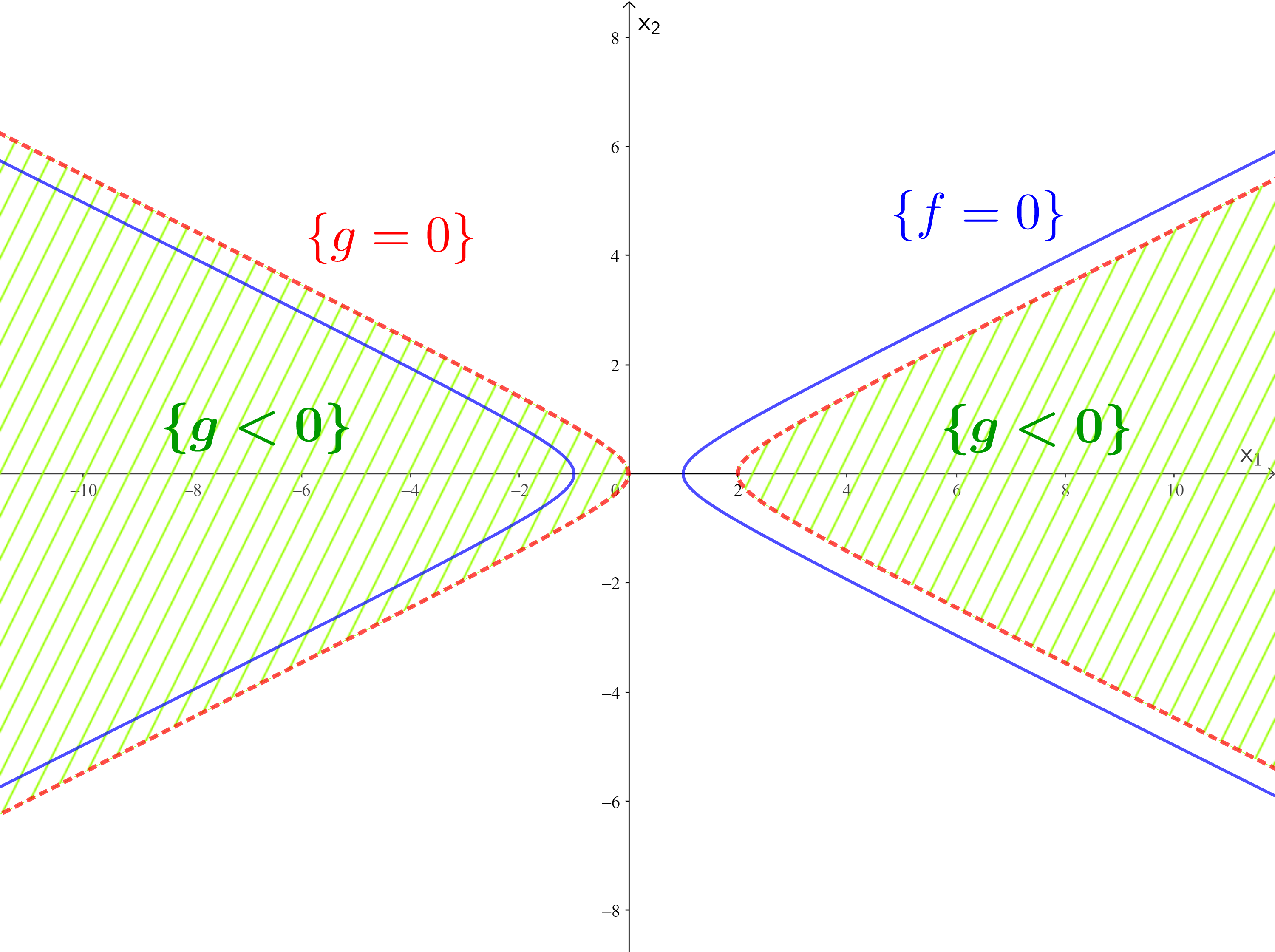
a The level set $\{g=0\}$ separates $\{f=0\}$ since one branch of $\{f=0\}$ lies in $\{g<0\}$ while the other lies in $\{g>0\}$.

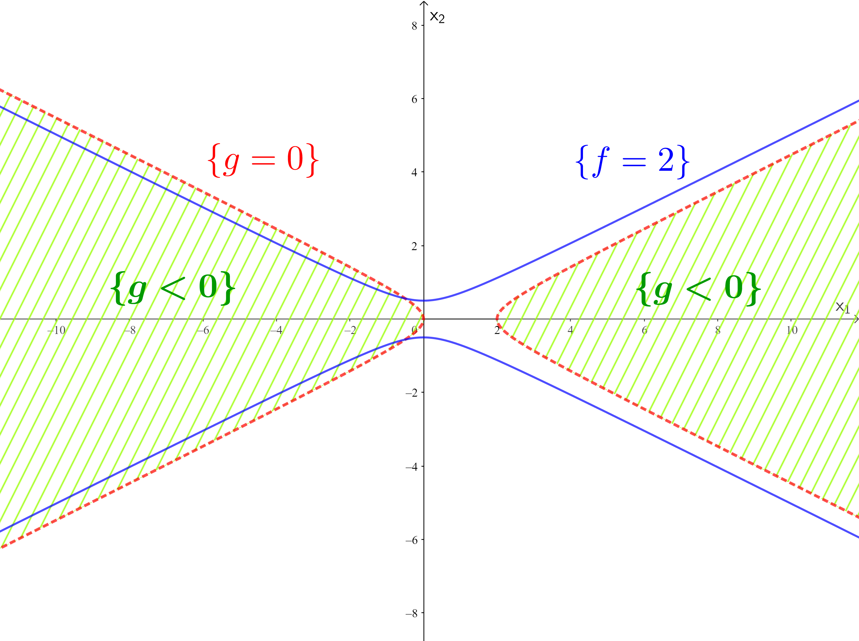
b Since $\{g=0\}\cap\{f=2\}\not=\emptyset,$ $\{g=0\}$ does not separate $\{f=2\}$ and $\{f=2\}$ does not separate $\{g=0\}$ either.

Figure 5: For remark (f) in which $f(x,y)=-x^{2}+4y^{2}+1$ and $g(x,y)=-(x-1)^{2}+4y^{2}+1$.

In the above remarks, four types of separation were considered.

• $\{g=0\}$ separates $\{f<0\}$;

• $\{g=0\}$ separates $\{f=0\}$;

• $\{g=0\}$ separates $\{f=0\}$, and simultaneously $\{f=0\}$ separates $\{g=0\}.$

• $\{g=\alpha\}$ separates $\{f=\beta\}$ for some $\alpha,\beta\in\mathbb{R}.$

For $\{g=0\}$ to separate $\{f<0\},$ it has been completely characterized by Nguyen and Sheu [7, 2019]. They showed that $\{g=0\}$ can separate $\{f<0\}$ if and only if $g$ is affine, the matrix $A$ (of $f$) has exactly one negative eigenvalue, and $f\left|{}_{\{g=0\}}(x)\right.\geq 0$, where $f\left|{}_{\{g=0\}}(x)\right.$ is the restriction of the function $f$ on the set $\{g=0\}$.

The case for $\{g=0\}$ to separate $\{f=0\}$ is quite different. While $\{g=0\}$ to separate $\{f<0\}$ can happen only when $g$ is affine, Figure 5a demonstrates the possibility for a quadratic level set $\{g=0\}$ to separate another quadratic level set $\{f=0\}.$ Interestingly, in an unpublished manuscript by Nguyen and Sheu [8, 2020], it was shown that, for $\{g=0\}$ to separate $\{f=0\},$ there must exist a linear combination $-\lambda f+g$ such that $-\lambda f+g$ is affine and $\{-\lambda f+g=0\}$ separates $\{f=0\}.$

Lemma 2.1 (Nguyen and Sheu [8, 2020]).

The 0-level set $\{g=0\}$ separates $\{f=0\}$ if and only if there exists some $\lambda\in\mathbb{R}$ such that $B=\lambda A$ and $\{-\lambda f+g=0\}$ separates $\{f=0\}$.

Lemma 2.1 limits $\{g=0\}$ to separate $\{f=0\}$ for only two cases. Due to $\{f=0\}$ being separated, it must be disconnected so that it is of a hyperbolic type (under a suitable basis) adopting either the following form

$$f(x)=-x_{1}^{2}+\delta(x_{2}^{2}+\cdots+x_{m}^{2})+1,~\delta\in\{0,1\};$$

or

$$f(x)=x_{1}^{2}-\delta(x_{2}^{2}+\cdots+x_{m}^{2})-1,~\delta\in\{0,1\}.$$

See Nguyen and Sheu [8, 2020]. By Lemma 2.1, when $\{g=0\}$ separates $\{f=0\}$, we know $B=\lambda A$ so that $g$ is either affine (in case $\lambda=0$), or is also of a hyperbolic type like $f$ (in case $\lambda\not=0$). The former one results in an affine level set $\{g=0\}$ to separate a hyperbolic level set $\{f=0\}$ as illustrated by Figure 4. The letter is a case that a hyperbolic level set $\{g=0\}$ separates another hyperbolic level set $\{f=0\}.$ See Figure 5a for an example. In either case, Lemma 2.1 reduces the separation of $\{f=0\}$ by $\{g=0\}$ to the separation of $\{f=0\}$ by a hyperplane $\{-\lambda f+g=0\}$ with a proper parameter $\lambda.$ The following lemma characterizes the necessary and sufficient conditions for an affine level set to separate a quadratic level set.

Lemma 2.2 (Nguyen and Sheu [8, 2020]).

Suppose that $h(x)=c^{T}x+c_{0}$ is affine. Then $\{h=0\}$ separates $\{f=0\}$ if and only if either $\left(\bar{f},\bar{A},\bar{a}\right)=\left(f,A,a\right)$ or $\left(\bar{f},\bar{A},\bar{a}\right)=\left(-f,-A,-a\right)$ satisfies the following three conditions:

1. $\bar{A}$ has exactly one negative eigenvalue, $\bar{a}\in\mathcal{R}(\bar{A})$

2. $c\in\mathcal{R}(\bar{A})$, $c\neq 0$

3. $V^{T}\bar{A}V\succeq 0$, $\bar{w}\in\mathcal{R}(V^{T}\bar{A}V)$, and $\bar{f}(x_{0})-\bar{w}^{T}(V^{T}\bar{A}V^{T})^{\dagger}\bar{w}>0$,

where $\bar{w}=V^{T}(\bar{A}x_{0}+\bar{a})$, $x_{0}=\frac{-c_{0}}{c^{T}c}c$, and $V\in\mathbb{R}^{n\times(n-1)}$ is the matrix basis for $\mathcal{N}(c^{T})$.

Furthermore, when it happens that a hyperbolic level set $\{g=0\}$ separates another hyperbolic level set $\{f=0\},$ as Figure 5a suggests, the reverse that $\{f=0\}$ separates $\{g=0\}$ also holds true.

Lemma 2.3 (Nguyen and Sheu [8, 2020]).

Suppose that both $f$ and $g$ are quadratic functions. If $\{g=0\}$ separates $\{f=0\}$, then $\{f=0\}$ separates $\{g=0\}$ also.

In the case of Lemma 2.3, we say that $\{g=0\}$ and $\{f=0\}$ mutually separate.

The following proposition shows that the separation property can be preserved under linear combinations.

Proposition 1.

If $\{g=0\}$ separates $\{f=0\}$, then $\{\eta f+\theta g=0\}$ separates $\{\sigma f=0\}$ for all $\eta,\theta,\sigma\in\mathbb{R}$ with $\theta\neq 0$, $\sigma\neq 0$.

Proof.

Since $\{g=0\}$ separates $\{f=0\}$, there are non-empty subsets $L^{+}$ and $L^{-}$ of $\{f=0\}$ such that

$$L^{-}\cup L^{+}=\{f=0\}~\text{ and }$$

$$g(u^{-})g(u^{+})<0,~\forall~u^{-}\in L^{-};~\forall~u^{+}\in L^{+}.$$

By $\{f=0\}=\{\sigma f=0\}$ for any $\sigma\neq 0,$ we have $L^{-}\cup L^{+}=\{\sigma f=0\}$. Moreover, for any $\theta\neq 0$,

$$(\eta f+\theta g)(u)(\eta f+\theta g)(v)=\theta^{2}g(u)g(v)<0~\text{ for all }u\in L^{+},v\in L^{-},$$

which shows that $\{\eta f+\theta g=0\}$ separates $\{\sigma f=0\}$ for all $\theta\neq 0$, $\sigma\neq 0$. ∎

The following proposition can be viewed as the converse of Proposition 1.

Proposition 2.

Suppose that $\{\eta f+\theta g=0\}$ separates $\{\sigma f+\tau g=0\}$ for some real numbers $\eta,\theta,\sigma,\tau$ with $\sigma\theta-\tau\eta\neq 0$. Then,

1. if both $f$ and $g$ are quadratic functions, the 0-level sets $\{f=0\}$ and $\{g=0\}$ mutually separate each other;

2. if one of $f$ and $g$ is an affine function, then the other must be a quadratic function and the affine 0-level set separates the quadratic 0-level set.

Namely, if $\{\eta f+\theta g=0\}$ separates $\{\sigma f+\tau g=0\}$ with $\sigma\theta-\tau\eta\neq 0$, then $\{g=0\}$ separates $\{f=0\}$ or $\{f=0\}$ separates $\{g=0\}$.

Proof.

Since $\{\eta f+\theta g=0\}$ separates $\{\sigma f+\tau g=0\}$, $\sigma f+\tau g$ cannot be affine function so that one of $f$ and $g$ is quadratic. Let us assume that $f$ is quadratic.

- If $\tau\neq 0$: by Proposition 1, we have

$$\left\{\frac{\theta}{\sigma\theta-\tau\eta}(\sigma f+\tau g)-\frac{\tau}{\sigma\theta-\tau\eta}(\eta f+\theta g)=0\right\}\hbox{ separates }\left\{\frac{1}{\tau}(\sigma f+\tau g)=0\right\}.$$

After simplifying,

$$\{f=0\}\text{ separates }\left\{\frac{\sigma}{\tau}f+g=0\right\}.$$

Since both $f$ and $\frac{\sigma}{\tau}f+g$ are quadratic, Lemma 2.3 ensures mutual separation so that $\{\frac{\sigma}{\tau}f+g=0\}$ separates $\{f=0\}$, too. Applying Proposition 1 again, we have $\{g=0\}$ separates $\{f=0\}$.

- If $\tau=0$: our assumption reduces to $\{\eta f+\theta g=0\}$ separates $\{\sigma f=0\}$. Since $\sigma\theta-\tau\eta\neq 0$, we have $\sigma\neq 0$ and $\theta\neq 0$. By Proposition 1,

$$\left\{-\frac{\eta}{\sigma\theta}(\sigma f)+\frac{1}{\theta}(\eta f+\theta g)=0\right\}\hbox{ separates }\left\{\frac{1}{\sigma}(\sigma f)=0\right\}.$$

It yields $\{g=0\}\text{ separates }\{f=0\}.$

Therefore, if a linear combination of $f$ and $g$ separates another linearly independent combination of them, and if $f$ is quadratic, we have $\{g=0\}$ separates $\{f=0\}$. Similarly, when $g$ is quadratic, we obtain $\{f=0\}$ separates $\{g=0\}$. In summary, under the assumption, we have

$$f\text{ is quadratic } \Longrightarrow\{g=0\}\text{ separates }\{f=0\}$$ (3)

$$g\text{ is quadratic } \Longrightarrow\{f=0\}\text{ separates }\{g=0\}.$$ (4)

Since one of $f$ and $g$ must be quadratic, one of (3) and (4) must happen. Hence,

• when both $f$ and $g$ are quadratic, $\{f=0\}$ and $\{g=0\}$ mutually separate;

• when one of $f$ and $g$ is affine, the affine 0-level set separates the quadratic 0-level set.

∎

Proposition 3.

The 0-level set $\{g=0\}$ separates the 0-level set $\{f=0\}$ if and only if

$$\{f=0\}\cap\{g=0\}=\emptyset~\text{ and }$$ (5)

$$g(u)g(v)<0~\text{ for some }~u,v\in\{f=0\}.$$ (6)

Proof.

The necessity follows directly from Definition 1. It suffices to prove the sufficiency. From (5), we know $\{f=0\}\subset\{g<0\}\cup\{g>0\}.$ Let

$$L^{-}=\{f=0\}\cap\{g<0\}~\text{ and }~L^{+}=\{f=0\}\cap\{g>0\}.$$ (7)

Due to (6), $L^{-}\not=\emptyset$ and $L^{+}\not=\emptyset$. Therefore, $\{f=0\}=L^{+}\cup L^{-}$. Finally, (7) directly implies that $g(u^{+})g(u^{-})<0$ for all $u^{+}\in L^{+}$ and $u^{-}\in L^{-}.$ The proof is complete. ∎

3 Characterising Non-convexity of $\mathbf{R}(f,g)$ by Separation of Level Sets

Now we are ready to show that the non-convexity of the joint range $\mathbf{R}(f,g)$ for two quadratic mappings, homogeneous or not, can be completely characterized by the separation feature of their level sets. This constitutes the main theme of the section.

Theorem 3.1.

The joint numerical range $\mathbf{R}(f,g)$ is non-convex if and only if there exists $\alpha,\beta\in\mathbb{R}$ such that $\{g=\beta\}$ separates $\{f=\alpha\}$ or $\{f=\alpha\}$ separates $\{g=\beta\}$. More precisely,

1. when both $f$ and $g$ are quadratic functions, $\mathbf{R}(f,g)$ is non-convex if and only if $(\exists\alpha,\beta\in\mathbb{R})~\{f=\alpha\}$ and $\{g=\beta\}$ mutually separates each other;

2. when one of $f$ and $g$ is affine, $\mathbf{R}(f,g)$ is non-convex if and only if $(\exists\alpha,\beta\in\mathbb{R})$ the affine $\beta$-level set separates the quadratic $\alpha$-level set.

Proof.

For convenience, let us adopt

$$\mathbf{R}(f,g)=\left\{(t,k)\in\mathbb{R}^{2}\left|~\begin{array}[]{r}t=f(x)\\ k=g(x)\end{array}~,~x\in\mathbb{R}^{n}\right.\right\}.$$

[Proof for necessity]: The set $\mathbf{R}(f,g)$ is non-convex if and only if there exists a triple of points $(M,N,K)$ satisfying

$$M,N\in\mathbf{R}(f,g),$$ (8)

$$M,N,K\text{ are colinear},$$ (9)

$$K\text{ lies between the segment }\overline{MN},$$ (10)

$$K\notin\mathbf{R}(f,g).$$ (11)

Figure 6: Graph for Proof of Theorem 3.1.

Let $L_{1}:\mu t+\nu k=p,~\mu^{2}+\nu^{2}\neq 0$ be the line passing through $M$, $N$, and $K$. Since both $M$ and $N$ lie in $L_{1}\cap\mathbf{R}(f,g)$, there exists some $u^{\ast},v^{\ast}$ such that $M=\left(f(u^{\ast}),g(u^{\ast})\right),~N=\left(f(v^{\ast}),g(v^{\ast})\right)$ and

$$u^{\ast},v^{\ast}\in\left\{x\in\mathbb{R}^{n}|~\mu f(x)+\nu g(x)=p\right\}.$$ (12)

Moreover, let $L_{2}:-\nu t+\mu k=s$ be perpendicular to $L_{1}$ with the intersection $K$. Since the two points $M$ and $N$ lie in different sides of $L_{2}$,

$$\left(-\nu f(u^{\ast})+\mu g(u^{\ast})-s\right)\left(-\nu f(v^{\ast})+\mu g(v^{\ast})-s\right)<0.$$ (13)

In addition, $K\not\in\mathbf{R}(f,g),$ we have

$$\left\{x\in\mathbb{R}^{n}|~\mu f(x)+\nu g(x)-p=0\right\}\cap\left\{x\in\mathbb{R}^{n}|-\nu f(x)+\mu g(x)-s=0\right\}=\emptyset.$$ (14)

Combining (12), (13), and (14) together, we apply Proposition 3 to conclude that

$$\{\mu f+\nu g=p\}~\hbox{ separates }~\{-\nu f+\mu g=s\}.$$ (15)

Since $\mu^{2}+\nu^{2}\neq 0$, (15) can be recast as

$$\left\{\mu\left(f-\alpha\right)+\nu(g-\beta)=0\right\}\text{ separates }\left\{-\nu(f-\alpha)+\mu\left(g-\beta\right)=0\right\},$$

where $\alpha=\frac{p\mu-s\nu}{\mu^{2}+\nu^{2}}$ and $\beta=\frac{p\nu+s\mu}{\mu^{2}+\nu^{2}}$. The nessesity part of the theorem follows immediately from Proposition 2.

[Proof for sufficiency]: Suppose that $\{g=\beta\}$ separates $\{f=\alpha\}$ for some $\alpha,\beta\in\mathbb{R}$. Proposition 3 implies that

$$\{g=\beta\}\cap\{f=\alpha\}=\emptyset$$ (16)

$$(g(u^{\ast})-\beta)(g(v^{\ast})-\beta)<0\text{ for some }u^{\ast},v^{\ast}\in\{f=\alpha\}.$$ (17)

Set the points $M,N,K$ as

$$M =\left(f(u^{\ast}),g(u^{\ast})\right)=\left(\alpha,g(u^{\ast})\right),~$$

$$N =\left(f(v^{\ast}),g(v^{\ast})\right)=\left(\alpha,g(v^{\ast})\right),~$$

$$K =\left(\alpha,\beta\right).$$

Then, $M,N,K$ lie on the same vertical line $t=\alpha$. Moreover, $M,N\in\mathbf{R}(f,g)$ and, by (17), $K$ lies between $M$ and $N.$ However, by (16), it is impossible to have $x\in\mathbb{R}^{n}$ such that $f(x)=\alpha$ and $g(x)=\beta$ so that $K\notin\mathbf{R}(f,g)$. Therefore, $\mathbf{R}(f,g)$ is non-convex. The other symmetry case that $\{f=\alpha\}$ separates $\{g=\beta\}$ for some $\alpha,\beta\in\mathbb{R}$ can be analogously proved. The proof of Theorem 3.1 is thus complete. ∎

Example 2.

Let two quadratic functions $f,~g$ be

$$f(x,y) =-\frac{\sqrt{3}}{2}x^{2}+\frac{\sqrt{3}}{2}y^{2}+x-\frac{1}{2}y$$

$$g(x,y) =\frac{1}{2}x^{2}-\frac{1}{2}y^{2}+\sqrt{3}x-\frac{\sqrt{3}}{2}y.$$

Figure 7a shows that $\{g=2\}$ and $\{f=-4\}$ mutually separate, and Figure 7b shows that the joint range $\mathbf{R}(f,g)$ is non-convex. These two figures justify our main theorem, Theorem 3.1.

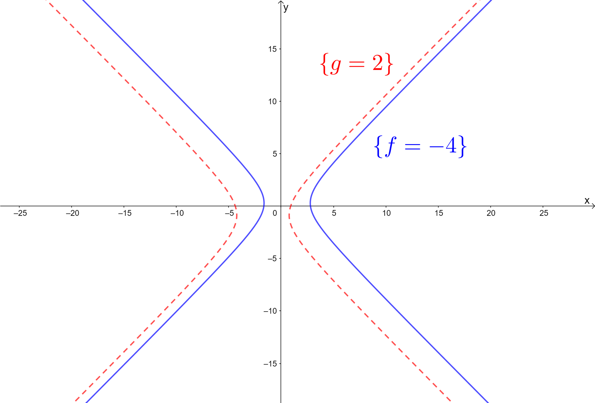
a The level set $\{g=2\}$ and the level set $\{f=-4\}$ mutually separate.

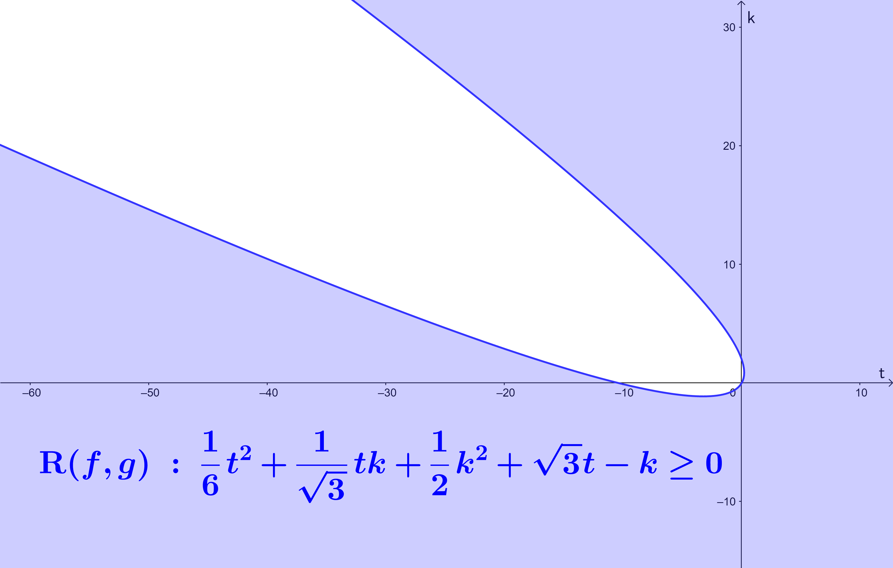
b The joint range $\mathbf{R}(f,g)$ is non-convex while $\{g=\beta\}$ and $\{f=\alpha\}$ mutually separate.

Figure 7: For Example 2. Let $f(x,y)=-\frac{\sqrt{3}}{2}x^{2}+\frac{\sqrt{3}}{2}y^{2}+x-\frac{1}{2}y$ and $g(x,y)=\frac{1}{2}x^{2}-\frac{1}{2}y^{2}+\sqrt{3}x-\frac{\sqrt{3}}{2}y$.

4 Algorithm for Checking Convexity of $\mathbf{R}(f,g)$

This section is devoted to a polynomial-time procedure for checking the convexity of $\mathbf{R}(f,g)$. If both $A$ and $B$ are zero, $\mathbf{R}(f,g)$ is the range of $\mathbb{R}^{n}$ under an affine transformation, which is convex. In the following, we assume that $A\neq 0.$ Then, Theorem 3.1 asserts that the joint range $\mathbf{R}(f,g)$ is non-convex if and only if there exists $\alpha,\beta\in\mathbb{R}$ such that

$$\{g-\beta=0\}\text{ separates }\{f-\alpha=0\}.$$ (18)

Lemma 2.1 further ensures that (18) can be always reduced, by suitable linear combinations of $f$ and $g$, to the case that an affine level set separates a quadratic one. Specifically, (18) holds if and only if the quadratic matrices of $g-\beta$ and $f-\alpha$ are linearly dependent, namely $B=\lambda A$, and the affine level set $\{-\lambda(f-\alpha)+(g-\beta)=0\}$ separates the quadratic level set $\{f-\alpha=0\}$. Thus, we obtain the following corollary of Theorem 3.1.

Corollary 1.

Suppose that $A\neq 0$. The joint numerical range $\mathbf{R}(f,g)$ is non-convex if and only if $B=\lambda A$ for some $\lambda\in\mathbb{R}$ and $\{-\lambda f+g=\gamma\}$ separates $\{f=\alpha\}$ for some $\alpha,\gamma\in\mathbb{R}$.

We observe that there are three constants in Corollary 1, $\lambda,~\gamma,~\alpha,$ the existence of which are to be determined. The condition “$B=\lambda A$ for some $\lambda\in\mathbb{R}$” is easy to verify. If $B\not=\lambda A,~\forall\lambda\in\mathbb{R},$ $\mathbf{R}(f,g)$ is convex. Otherwise, $\mathbf{R}(f,g)$ can be non-convex only when there exists some $\gamma,~\alpha$ such that the hyperplane $\{-\lambda f+g=\gamma\}$ separates $\{f=\alpha\}$. By Lemma 2.2, such a pair of $\gamma,\alpha$, if exist, must satisfy the following: either $\left(\bar{f}_{\alpha},\bar{A},\bar{a}\right)=\left(f-\alpha,A,a\right)$ or $\left(\bar{f}_{\alpha},\bar{A},\bar{a}\right)=\left(-\left(f-\alpha\right),-A,-a\right)$ satisfies

1. $\bar{A}$ has exactly one negative eigenvalue, $\bar{a}\in\mathcal{R}(\bar{A})$

2. $c=-\lambda a+b\in\mathcal{R}(\bar{A})$, $c\neq 0$

3. $V^{T}\bar{A}V\succeq 0$, $\bar{w}_{\gamma}\in\mathcal{R}(V^{T}\bar{A}V)$, and $\bar{f}_{\alpha}(x_{\gamma})-\bar{w}_{\gamma}^{T}(V^{T}\bar{A}V^{T})^{\dagger}\bar{w}_{\gamma}>0$,

where $\bar{w}_{\gamma}=V^{T}(\bar{A}x_{\gamma}+\bar{a})$, $x_{\gamma}=\frac{-(-\lambda a_{0}+b_{0}-\gamma)}{c^{T}c}c$, and $V\in\mathbb{R}^{n\times(n-1)}$ is the matrix basis for $\mathcal{N}(c^{T})$.

However, among (i)-(iii), we find that $\alpha,~\gamma$ appear only in

$$\bar{w}_{\gamma}\in\mathcal{R}(V^{T}\bar{A}V),~\bar{w}_{\gamma}=V^{T}(\bar{A}x_{\gamma}+\bar{a}),~x_{\gamma}=\frac{-(-\lambda a_{0}+b_{0}-\gamma)}{c^{T}c}c$$ (19)

$$\bar{f}_{\alpha}(x_{\gamma})-\bar{w}_{\gamma}^{T}(V^{T}AV^{T})^{\dagger}\bar{w}_{\gamma}>0.$$ (20)

where $\left(\bar{f}_{\alpha},\bar{A},\bar{a}\right)=\left(f-\alpha,A,a\right)$ or $\left(\bar{f}_{\alpha},\bar{A},\bar{a}\right)=\left(-\left(f-\alpha\right),-A,-a\right)$. Moreover, we observe that (20) depends on (19). As long as there exists $\gamma$ such that (19) holds, one can choose $\alpha$ to be small enough (when $\bar{f}_{\alpha}=f-\alpha$) or large enough (when $\bar{f}_{\alpha}=-\left(f-\alpha\right)$) so that (20) follows immediately. In the next lemma, we show that the existence of $\gamma$ satisfying (19) can be guaranteed by “$\bar{a}\in\mathcal{R}(\bar{A})$” in (i), and hence the problem for the existence of $\alpha,~\gamma$ can be reduced to checking the following conditions (B1)-(B3).

Lemma 4.1.

Let $h(x)=c^{T}x+c_{0}$ be an affine function and $f(x)=x^{T}Ax+2a^{T}x+a_{0}$ be a quadratic function. The following statements are equivalent:

1. The level set $\{h=\gamma\}$ separates the level set $\{f=\alpha\}$ for some $\alpha,\gamma\in\mathbb{R}$.

2. The matrix $\bar{A}=A$ or $\bar{A}=-A$ satisfies the following three conditions:

   1. $\bar{A}$ has exactly one negative eigenvalue, $a\in\mathcal{R}(A)$

   2. $c\in\mathcal{R}(A)$, $c\neq 0$

   3. $V^{T}\bar{A}V\succeq 0$

   where $V\in\mathbb{R}^{n\times(n-1)}$ is a matrix basis of $\mathcal{N}(c^{T})$.

Proof.

As we say above, according to Lemma 2.2, the level set $\{h=\gamma\}$ separates $\{f=\alpha\}$ for some $\alpha,\gamma\in\mathbb{R}$ if and only if there exist $\gamma,\alpha$ satisfying conditions (i)-(iii) mentioned above for either $\left(\bar{f}_{\alpha},\bar{A},\bar{a}\right)=\left(f-\alpha,A,a\right)$ or $\left(\bar{f}_{\alpha},\bar{A},\bar{a}\right)=\left(-\left(f-\alpha\right),-A,-a\right)$.

In either cases, one has

$$\bar{a}\in\mathcal{R}(\bar{A})~ \Leftrightarrow~a\in\mathcal{R}(A)$$ (21)

$$c\in\mathcal{R}(\bar{A})~ \Leftrightarrow~c\in\mathcal{R}(A)$$ (22)

Therefore, when $\left(\bar{f}_{\alpha},\bar{A},\bar{a}\right)$ satisfies (i)-(iii), the same $\bar{A}$ must satisfy conditions (B1)-(B3). Hence, statement (a) directly implies statement (b).

To prove the converse, we take $\bar{a}=a$, $\bar{f}_{\alpha}=f-\alpha$ if $\bar{A}=A$ and take $\bar{a}=-a$, $\bar{f}_{\alpha}=-\left(f-\alpha\right)$ if $\bar{A}=-A$, where $\alpha$ is a constant which will be determined later. With this choice of the triple $(\bar{f}_{\alpha},\bar{A},\bar{a})$, the equivalences (21) and (22) together imply that (i) and (ii) hold true. Finally, it suffices to show the existence of $\alpha,\gamma$ satisfying (iii). We have mentioned that the existence of $\alpha$ depends on the existence of $\gamma$, and then it suffices to show that “$\bar{a}\in\mathcal{R}(\bar{A})$” guarantees the existence of $\gamma$ satisfying

$$\bar{w}_{\gamma}\in\mathcal{R}(V^{T}\bar{A}V),~\bar{w}_{\gamma}=V^{T}(\bar{A}x_{\gamma}+\bar{a}),~x_{\gamma}=\frac{-(c_{0}-\gamma)}{c^{T}c}c.$$ (23)

Since $\bar{a}\in\mathcal{R}(\bar{A})$, there exists some $u_{0}\in\mathbb{R}^{n}$ such that

$$V^{T}\bar{a}=V^{T}\bar{A}u_{0}.$$ (24)

As $V\in\mathbb{R}^{n\times(n-1)}$ is a matrix basis for $\mathcal{N}(c^{T})$, the $n\times n$ matrix $\left({V},\frac{1}{{c}^{T}{c}}{c}\right)$ is of full rank. Thus, for $u_{0}$ in (24), there exists $y\in\mathbb{R}^{n-1}$ and $\gamma_{0}\in\mathbb{R}$ such that

$$u_{0}=\left(V,\frac{1}{c^{T}c}c\right)\left(\begin{array}[]{c}y\\ \gamma_{0}\end{array}\right)=Vy+\frac{\gamma_{0}}{c^{T}c}c.$$ (25)

Take $\gamma=c_{0}-\gamma_{0}$. Equations (24) and (25) thus imply

$$\begin{split}V^{T}\bar{a}&=V^{T}\bar{A}Vy+\frac{\gamma_{0}}{c^{T}c}V^{T}\bar{A}c\\ &=V^{T}\bar{A}Vy+\frac{(c_{0}-\gamma)}{c^{T}c}V^{T}\bar{A}c\\ &=V^{T}\bar{A}Vy-V^{T}\bar{A}x_{\gamma}\end{split}$$

Hence, we obtain

$$V^{T}\bar{A}Vy=V^{T}\bar{a}+V^{T}\bar{A}x_{\gamma}=\bar{w}_{\gamma},$$

which shows that such taken $\gamma$ satisfies (23), and hence the existence of $\alpha$ follows. The proof is therefore completed. ∎

Combining Corollary 1 with Lemma 4.1 all together, we see that, if $A\neq 0$, the joint range $\mathbf{R}(f,g)$ is non-convex when and only when the following two parts are satisfied:

• $A$ and $B$ are linearly dependent, say $B=\lambda A$;

• two constants $\alpha,~\gamma$ can be chosen so that the hyperplane $\{-\lambda f+g=\gamma\}$ separates the quadratic hypersurface $\{f=\alpha\},$ which can be checked by (B1)-(B3),

We write this into the following main theorem, which can be converted into a numerical procedure for checking the convexity of $\mathbf{R}(f,g)$.

Theorem 4.2.

Given two quadratic functions $f(x)=x^{T}Ax+2a^{T}x+a_{0}$ and $g(x)=x^{T}Bx+2b^{T}x+b_{0}$ with $A\neq 0$. The joint numerical range $\mathbf{R}(f,g)$ is non-convex if and only if the matrix $\bar{A}=A$ or $\bar{A}=-A$ satisfies the following four:

1. $B=\lambda A$ for some $\lambda\in\mathbb{R}$

2. $\bar{A}$ has exactly one negative eigenvalue, $a\in\mathcal{R}(A)$

3. $-\lambda a+b\in\mathcal{R}(A)$, $-\lambda a+b\neq 0$

4. $V^{T}\bar{A}V\succeq 0$

where $V\in\mathbb{R}^{n\times(n-1)}$ is a matrix basis of $\mathcal{N}((-\lambda a+b)^{T})$.

The procedure is described below by a few steps. Notice that each step can be implemented in polynomial time. An implementable pseudo-code is also provided in Algorithm 1 in the next page.

Given

The coefficient matrices $A$, $B$, $a$, and $b$.

Step 0

Check whether $A=B=0$ or $a=b=0$.

• If true, then $\mathbf{R}(f,g)$ is convex.

• If false, go to next step. (Without loss of generality, we assume $A\neq 0$ in the following.)

Step 1

Check whether $B=\lambda A$ for some $\lambda$ in $\mathbb{R}$.

• If true, set $c=-\lambda a+b$ and go to next step.

• If false, then $\mathbf{R}(f,g)$ is convex.

Step 2

Check whether $c\neq 0$ and whether both the linear systems $Ay_{1}=a$ and $Ay_{2}=c$ have solutions.

• If true, set $V\in\mathbb{R}^{n\times(n-1)}$ to be the matrix basis of $\mathcal{N}(c^{T})$ and go to next step.

• If false, then $\mathbf{R}(f,g)$ is convex.

Step 3

Check whether one of the following cases happens:

(a) $$A\text{ has exactly one negative eigenvalue and }V^{T}AV\succeq 0$$

(b) $$A\text{ has exactly one positive eigenvalue and }V^{T}AV\preceq 0$$

• If one of (a) and (b) holds, then $\mathbf{R}(f,g)$ is non-convex.

• Otherwise, $\mathbf{R}(f,g)$ is convex.

input : The coefficient matrices $A$, $B$, $a$, $b$

output : Convexity or non-convexity of $\mathbf{R}(f,g)$

if $A=B=0~$ or $~a=b=0$ then

    return convex ;

   

else if $A=0~$ and $~B\neq 0$ then

    $A\leftarrow B$ ;

     /* Always set $A$ to be the non-zero matrix */

    $B\leftarrow 0$ ;

   

end if

if $B=\lambda A$ for some $\lambda\in\mathbb{R}$ then

    $c\leftarrow-\lambda a+b$;

    if $c\neq 0$ then

       if Both linear systems $Ay_{1}=a$ and $Ay_{2}=c$ have solutions then

          $V\leftarrow$ matrix basis for null space of $c^{T}$ ;

           /* $V$ is an $n\times(n-1)$ matrix */

          if $A$ has exactly one negative eigenvalue and $V^{T}AV\succeq 0$ then

             return non-convex;

            

          else if $A$ has exactly one positive eigenvalue and $V^{T}AV\preceq 0$ then

             return non-convex;

            

          end if

         

       end if

      

    end if

   

end if

return convex;

Algorithm 1 Algorithm for checking the convexity of $\mathbf{R}(f,g)$

Example 3.

Let $f(x)=x^{T}Ax+2a^{T}x$ and $g(x)=x^{T}Bx+2b^{T}x$ be two quadratic functions on $\mathbb{R}^{n}$ with coefficient matrices

$$\begin{split}&A=\left[\begin{array}[]{c c c c}0&0&-1&0\\ 0&\frac{1}{2}&0&\frac{1}{2}\\ -1&0&0&0\\ 0&\frac{1}{2}&0&\frac{1}{2}\end{array}\right]\ ,\ B=\left[\begin{array}[]{c c c c}0&0&-2&0\\ 0&1&0&1\\ -2&0&0&0\\ 0&1&0&1\end{array}\right]\\ &2a=\left(2,\sqrt{2},2,\sqrt{2}\right)^{T},2b=\left(5,\frac{3}{\sqrt{2}},8,\frac{3}{\sqrt{2}}\right)^{T}\end{split}$$

Step 0

Neither $A=B=0$ nor $a=b=0$.

Step 1

Observe that $B=\lambda A$ with $\lambda=2$. Set

$$c^{T}=-\lambda a+b=\left(1,\frac{-1}{\sqrt{2}},4,\frac{-1}{\sqrt{2}}\right)$$

Step 2

One has $c\neq 0$. Both systems $Ay_{1}=a$ and $Ay_{2}=c$ have solutions:

$$y_{1}=\left[\begin{array}[]{c}-1\\ \frac{1}{\sqrt{2}}\\ -1\\ \frac{1}{\sqrt{2}}\end{array}\right]~\text{ and }~y_{2}=\left[\begin{array}[]{c}-2\\ \frac{-1}{2\sqrt{2}}\\ \frac{-1}{2}\\ \frac{-1}{2\sqrt{2}}\end{array}\right]$$

Step 3

Four eigenvalues of $A$ are $\lambda_{1}=-1,\ \lambda_{2}=0,\ \lambda_{3}=\lambda_{4}=1.$ Thus, $A$ has exactly one negative eigenvalue. We may choose $V\in\mathbb{R}^{n\times(n-1)}$ be the matrix basis of $\mathcal{N}(c^{T})$ such that

$$V=\left[\begin{array}[]{c c c}\frac{1}{\sqrt{2}}&-4&\frac{1}{\sqrt{2}}\\ 1&0&0\\ 0&1&0\\ 0&0&1\end{array}\right]~\text{ and }~V^{T}AV=\left[\begin{array}[]{c c c}\frac{1}{2}&\frac{-1}{\sqrt{2}}&\frac{1}{2}\\ \frac{-1}{\sqrt{2}}&8&\frac{-1}{\sqrt{2}}\\ \frac{1}{2}&\frac{-1}{\sqrt{2}}&\frac{1}{2}\\ \end{array}\right].$$

The matrix $V^{T}AV$ has eigenvalues $\eta_{1}=0,\ \eta_{2}=\frac{9-\sqrt{53}}{2},\ \eta_{3}=\frac{9+\sqrt{53}}{2}$, which are all non-negative. Hence, $V^{T}AV$ is positive semidefinite. Therefore, we conclude that the joint range $\mathbf{R}(f,g)$ is non-convex.

The shaded region in Figure 8 is $\mathbf{R}(f,g)$ of this example, which justifies our procedure.

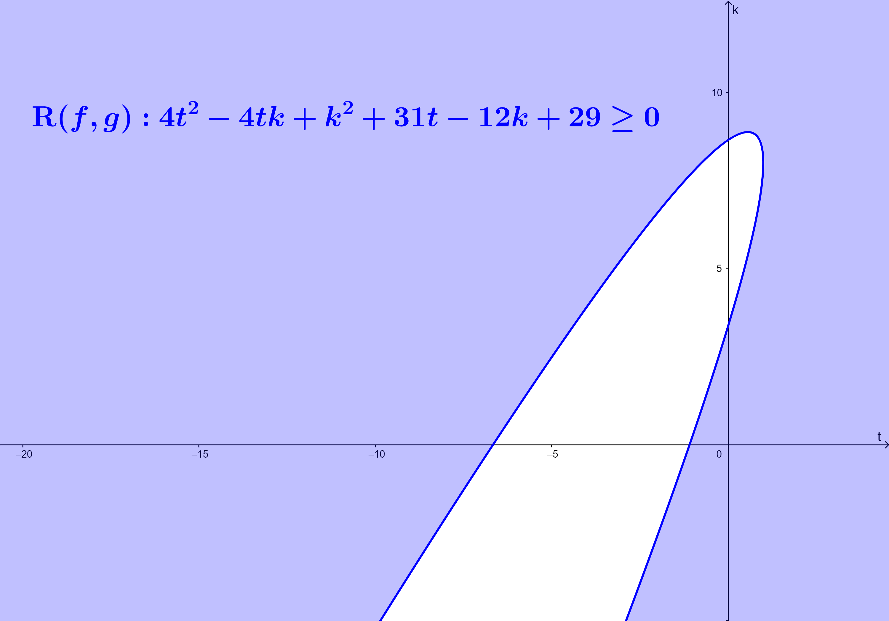
Figure 8: The joint numerical range $\mathbf{R}(f,g)$ in Example 3.

5 Implications

In this section, we show that the necessary and sufficient conditions for the convexity of $\mathbf{R}(f,g)$ developed by Flores-Bazán and Opazo [4, 2016] is a direct consequence of our Theorem 3.1. For convenience, we list their result as Theorem 5.1 below.

Theorem 5.1 (Flores-Bazán and Opazo [4, 2016]).

The joint numerical range $\mathbf{R}(f,g)$ is non-convex if and only if there exists some $d=(d_{1},d_{2})\in\mathbb{R}^{2}$, $d\neq 0$ such that the following four hold:

1. $a,~b\in\left(\mathcal{N}(A)\cap\mathcal{N}(B)\right)^{\perp}$

2. $d_{2}A=d_{1}B$

3. $-d\in\mathbf{R}(f_{H},g_{H})$

4. $F_{H}(u)=-d\implies\left\langle F_{L}(u),d_{\perp}\right\rangle\neq 0$

where $F_{H}(x)=\left(f_{H}(x),g_{H}(x)\right)=\left(x^{T}Ax,x^{T}Bx\right)$, $F_{L}(x)=\left(a^{T}x,b^{T}x\right)$, and $d_{\perp}=(-d_{2},d_{1})$.

As we can see, Theorem 5.1 verifies whether $\mathbf{R}(f,g)$ is non-convex by the existence of a certificate $d=(d_{1},d_{2})\not=0$ satisfying conditions (C1)-(C4), but Flores-Bazán and Opazo in [4, 2016] did not provide a procedure for providing such a certificate. In addition, even with a certificate $d=(d_{1},d_{2})\not=0$ on hand, conditions (C1)-(C4) reveal very little information as to what was going on behind the scenes.

Our approach reduces the non-convexity of $\mathbf{R}(f,g)$ to also checking the existence of two constants $\alpha,\beta$ such that $\{f=\alpha\}$ separates $\{g=\beta\}$ or reversely. Then, from Theorem 4.2, there are four possibilities which could happen:

• $A$ has exactly one negative eigenvalue ($\{g=\beta\}$ separates $\{f=\alpha\}$);

• $A$ has exactly one positive eigenvalue ($\{g=\beta\}$ separates $\{f=\alpha\}$);

• $B$ has exactly one negative eigenvalue ($\{f=\alpha\}$ separates $\{g=\beta\}$);

• $B$ has exactly one positive eigenvalue ($\{f=\alpha\}$ separates $\{g=\beta\}$).

In the following, we can show that, if $\mathbf{R}(f,g)$ is non-convex, condition (C3) in Theorem 5.1 can be strengthened to conclude that there exists either a positive eigenvalue or a negative eigenvalue for the $A$ matrix or the $B$ matrix, while there is only one positive (or only one negative) eigenvalue can be derived from condition (C4). In other words, our Theorem 3.1, or equivalently, Theorem 4.2 provide more detail information than (C1)-(C4) did, and thus the latter can be put as a consequence of the former. Though we know the two are actually equivalent, yet coming back from (C1)-(C4) to conclude our separation property Theorem 3.1 is perhaps non-trivial.

Theorem 5.2.

Let $f(x)=x^{T}Ax+2a^{T}x+a_{0}$ and $g(x)=x^{T}Bx+2b^{T}x+b_{0}$ be two quadratic functions defined on $\mathbb{R}^{n}$ and $B=\lambda A$ for some $\lambda\in\mathbb{R}.$ If the level set $\{g=\beta\}$ separates $\{f=\alpha\}$ for some $\alpha,\beta\in\mathbb{R}$, then $d_{+}=(1,\lambda)\in\mathbb{R}^{2}$ or $d_{-}=(-1,-\lambda)\in\mathbb{R}^{2}$ satisfy Conditions (C1)-(C4) in Theorem 5.1.

Proof.

Since $B=\lambda A$, Condition (C2) holds for both $d_{+}=(1,\lambda)$ and $d_{-}=(-1,-\lambda)$. When $\{g=\beta\}$ separates $\{f=\alpha\}$ for some $\alpha,\beta\in\mathbb{R}$, the function $f$ cannot be affine, and hence $A\neq 0$. Also, according to Lemma 2.1, when $B=\lambda A$ and $\{g=\beta\}$ separates $\{f=\alpha\}$, the hyperplane $\{-\lambda(f-\alpha)+(g-\beta)=0\}$ also separates $\{f=\alpha\}$. Hence, Lemma 4.1 ensures the following three conditions hold:

1. $A$ has exactly one negative (resp. positive) eigenvalue, $a\in\mathcal{R}(A)$

2. $c=-\lambda a+b\in\mathcal{R}(A)$, $c\neq 0$

3. $V^{T}AV\succeq 0$ (resp. $\preceq 0$)

where $V\in\mathbb{R}^{n\times(n-1)}$ is a matrix basis of $\mathcal{N}(c^{T})$. In the following, we will show that Conditions (B1)-(B3) imply that $d_{+}=(1,\lambda)$ or $d_{-}=(-1,-\lambda)$ satisfies Conditions (C1), (C3), and (C4).

Note that (C1) is independent to the choice of $d$, so we verify it first. Since $A$ is symmetric, we obtain

$$\mathcal{R}(A)=\mathcal{R}(A^{T})=\mathcal{N}(A)^{\perp}.$$

Also, when $B=\lambda A$, we have $\mathcal{N}(A)\cap\mathcal{N}(B)=\mathcal{N}(A),$ and hence

$$\mathcal{R}(A)=\left(\mathcal{N}(A)\cap\mathcal{N}(B)\right)^{\perp}.$$

Thus, (B1) and (B3) imply that $a,~b\in\mathcal{R}(A)=\left(\mathcal{N}(A)\cap\mathcal{N}(B)\right)^{\perp}$, which means (C1) holds. For Conditions (C3) and (C4), we divide into two cases according Conditions (B1) and (B3):

When $A$ has exactly one negative eigenvalue and $V^{T}AV\succeq 0$, we are going to show that $d_{+}=(1,\lambda)$ satisfies (C3) and (C4). For (C3), since $A$ has one negative eigenvalue, there exists $u\in\mathbb{R}^{n}$ such that $u^{T}Au=-1$, and hence $u^{T}Bu=-\lambda$ due to relation $B=\lambda A$. Therefore, $F_{H}(u)=-d_{+}$, which means $d_{+}$ satisfies (C3). To show Condition (C4) holds for $d_{+}=(1,\lambda)$, it suffices to show the following implications:

$$\left\langle F_{L}(u),(d_{+})_{\perp}\right\rangle=0~\implies~F_{H}(u)\neq-d_{+}.$$ (26)

Observe that

$$\left\langle F_{L}(u),(d_{+})_{\perp}\right\rangle=-\lambda a^{T}u+b^{T}u=c^{T}u.$$

Now, for any $u\in\mathbb{R}^{n}$ such that $\left\langle F_{L}(u),(d_{+})_{\perp}\right\rangle=0$, one has $u\in\mathcal{N}(c^{T})$. Then there exists some $w\in\mathbb{R}^{n-1}$ such that $u=Vw$. Since $V^{T}AV\succeq 0$, we have

$$u^{T}Au=w^{T}V^{T}AVw\geq 0,$$

which implies that $u^{T}Au\neq-1$, and hence $F_{H}(u)\neq-d_{+}$. Therefore, (26) holds, which means $d_{+}$ satisfies Condition (C4).

When $A$ has exactly one positive eigenvalue and $V^{T}AV\preceq 0$, similar argument will ensure that $d_{-}=(-1,-\lambda)$ satisfies Conditions (C3) and (C4). ∎

6 Conclusion

In this paper, we convert the problem about the convexity of $\mathbf{R}(f,g)$ in codomain into the separation property of level sets in the domain. The geometric feature for the non-convexity of the joint numerical range of two quadratic functions $f$ and $g$ is that there exists a pair of level sets $\{g=\beta\}$ and $\{f=\alpha\}$ such that $\{g=\beta\}$ separates $\{f=\alpha\}$ or $\{f=\alpha\}$ separates $\{g=\beta\}$. The result also suggests that S-lemma with equality by Xia et al. [13, 2016] is also a direct consequence of the convexity of $\mathbf{R}(f,g)$. By Nguyen and Sheu [7, 2019], under Slater condition, the S-lemma with equality fails if and only if $\{g=0\}$ separates $\{f<0\}$. Hence, $f$ must have exactly one negative eigenvalue and thus $\{g=0\}$ separates $\{f=-1\}.$ Finally, our approach also lends itself to a polynomial time procedure for checking the convexity of $\mathbf{R}(f,g),$ which we believe to facilitate more applications in the future.

References

- [1] L. Brickmen, On the Field of Values of a Matrix, Proceedings of the American Mathematical Society, 12 (1941), 61–66.
- [2] L. L. Dines, On the mapping of quadratic forms, Bulletin of the American Mathematical Society, 47 (1941), 494–498.
- [3] K. Derinkuyu and M. Ç. Pınar, On the S-procedure and some variants, Mathematical Methods of Operations Research, 64 (2006), 55–77.
- [4] F. A. B. I. Á. N. Flores-Bazán and F. Opazo, Characterizing the convexity of joint-range for a pair of inhomogeneous quadratic functions and strong duality, Minimax Theory Appl, 1 (2016), 257–290.
- [5] S. C. Fang, D. Y. Gao, G. X. Lin, R. L. Sheu and W. X. Xing, Double well potential function and its optimization in the n-dimensional real space–Part I, J. Ind. Manag. Optim., 13 (2017), 1291–1305.
- [6] H. Q. Nguyen, R. L. Sheu and Y. Xia, Solving a new type of quadratic optimization problem having a joint numerical range constraint, 2020. Available from: https://doi.org/10.13140/RG.2.2.23830.98887.
- [7] H. Q. Nguyen and R. L. Sheu, Geometric properties for level sets of quadratic functions, Journal of Global Optimization, 73 (2019), 349–369.
- [8] H. Q. Nguyen and R. L. Sheu, Separation properties of quadratic functions, 2020. Available from: https://doi.org/10.13140/RG.2.2.18518.88647.
- [9] B. T. Polyak, Convexity of quadratic transformations and its use in control and optimization, Journal of Optimization Theory and Applications, 99 (1998), 553–583.
- [10] I. Pólik and T. Terlaky, A survey of the S-lemma, SIAM review, 49 (2007), 371–418.
- [11] M. Ramana and A. J. Goldman, Quadratic maps with convex images, Submitted to Math of OR.
- [12] H. Tuy and H. D. Tuan, Generalized S-lemma and strong duality in nonconvex quadratic programming, Journal of Global Optimization, 56 (2013), 1045–1072.
- [13] Y. Xia, S. Wang and R. L. Sheu, S-lemma with equality and its applications, Mathematical Programming, 156 (2016), 513–547.
- [14] Y. Xia, R. L. Sheu, S. C. Fang and W. Xing, Double well potential function and its optimization in the n-dimensional real space–Part II, J. Ind. Manag. Optim., 13 (2017), 1307–1328.
- [15] V. A. Yakubovich, S-procedure in nolinear control theory, Vestnik Leninggradskogo Universiteta, Ser. Matematika, (1971), 62–77.
- [16] Y. Ye and S. Zhang, New results on quadratic minimization, SIAM Journal on Optimization, 14 (2003), 245–267.