Understanding Dataset Distillation via Spectral Filtering

Abstract

Dataset distillation (DD) has emerged as a promising approach to compress datasets and speed up model training. However, the underlying connections among various DD methods remain largely unexplored. In this paper, we introduce UniDD, a spectral filtering framework that unifies diverse DD objectives. UniDD interprets each DD objective as a specific filter function that affects the eigenvalues of the feature-feature correlation (FFC) matrix and modulates the frequency components of the feature-label correlation (FLC) matrix. In this way, UniDD reveals that the essence of DD fundamentally lies in matching frequency-specific features. Moreover, according to the filter behaviors, we classify existing methods into low-frequency matching and high-frequency matching, encoding global texture and local details, respectively. However, existing methods rely on fixed filter functions throughout distillation, which cannot capture the low- and high-frequency information simultaneously. To address this limitation, we further propose Curriculum Frequency Matching (CFM), which gradually adjusts the filter parameter to cover both low- and high-frequency information of the FFC and FLC matrices. Extensive experiments on small-scale datasets, such as CIFAR-10/100, and large-scale datasets, including ImageNet-1K, demonstrate the superior performance of CFM over existing baselines and validate the practicality of UniDD.

1 Introduction

The exponential growth of data presents significant challenges to the efficiency and scalability of training deep neural networks [ImageNet, CLIP, ViT, SAM]. Dataset distillation (DD) has emerged as a solution to these challenges, aiming to condense large-scale real datasets into compact, synthetic ones without compromising model performance [DD, DD_survey1, DD_survey2, DD_survey3, DD_survey4]. This approach has shown promise across a range of domains, including image [DC, DM, MTT], time series [TS1, TS2], and graph [GCOND, SGDD, GDEM].

Existing DD methods vary in their optimization objectives, which can be grouped into four main categories. Statistical matching [DM, IDM, CAFE] aligns key statistics, such as mean and variance, between real and synthetic datasets. Gradient matching [DC, IDC, DSA] minimizes the direction of model gradients across real and synthetic data during training. Trajectory matching [MTT, TESLA, FTD, DATM] enforces the synthetic data to emulate the update trajectories of real model parameters. Kernel-based approaches [KIP, FRePo, RFAD] employ closed-form representations to bypass the inner-optimization and improve distillation efficiency. Despite differences in their objectives, all methods strive to minimize the discrepancy between real and synthetic datasets from certain perspectives. This raises some key questions: Are these DD methods related? If so, is there a unified framework that can encompass and explain the objectives of various DD methods? These questions are crucial as a unified framework can deepen our understanding of DD, uncover the essence of existing methods, and offer potential insights for advanced distillation technologies.

As the first contribution of our work, we theoretically analyze some representative DD methods, including DM [DM], DC [DC], MTT [MTT], and FrePo [FRePo], and summarize them into a spectral filtering framework, termed UniDD, uncovering their commonalities and differences. Specifically, these DD methods are all proven to match the feature-feature correlation (FFC) and feature-label correlation (FLC) matrices between the real and synthetic datasets. Their difference lies in the filter function applied to the FFC matrix, which changes the eigenvalues of the FFC matrix to target certain frequency components of the FLC matrix.

Based on the differences in their filtering behaviors, we classify existing DD methods into two categories: low-frequency matching (LFM) and high-frequency matching (HFM). Our experimental investigations, detailed in Section 2.3, demonstrate that LFM-based methods, e.g., DM and DC, capture the global textures, while HFM-based methods, e.g., MTT and FrePo, focus on more fine-grained details. Notably, HFM usually outperforms LFM, suggesting that high-frequency information potentially plays a more significant role in achieving superior distillation performance.

The connections between DD objectives and filter functions further enable us to identify the weaknesses of existing methods. Traditional DD methods typically select the matching objectives based on intuition, while UniDD shifts this paradigm to filter design, making the new DD methods more interpretable and reliable. Based on the guidance of UniDD, we find that existing DD methods only use fixed filter functions during distillation, and can only cover a few frequency components, limiting their adaptability. Therefore, we propose Curriculum Frequency Matching (CFM), which gradually adjusts the filter parameter to increase the ratio of low-frequency information in the high-pass filter, thereby covering a wider range of frequency components. To verify its effectiveness, we conduct extensive experiments on various datasets, including CIFAR-10/100, Tiny-ImageNet, and ImageNet-1k. The results demonstrate that CFM consistently outperforms baselines by substantial margins and yields better cross-architecture generalization ability. The contributions of this paper are summarized below:

• We introduce UniDD, a spectral filtering framework that interprets each DD objective as a specific filter function applied to FFC and FLC matrices, thus unifying diverse DD methods as a frequency-matching problem.

• We classify existing methods into low-frequency and high-frequency matching based on their filter functions, highlighting their respective roles in encoding global textures and local details.

• We propose CFM, a novel DD method with dynamic filters that encode both low- and high-frequency information. Extensive experiments across diverse benchmarks demonstrate its superior performance over existing baselines.

Scope of UniDD.

The proposed framework mainly focuses on unifying the objectives of different DD methods, while other research lines, e.g., data parameterization and model augmentation, are beyond the scope of this paper, and we introduce them in the related work section.

2 A Unified Framework of Dataset Distillation

Notations. Let $\mathcal{T}=(H,Y)$ denote a real dataset, where $H$ represents the original data with $|H|=n$ samples, and $Y\in\mathbb{R}^{n\times c}$ is the one-hot label matrix for $c$ classes. The goal of DD is to learn a synthetic network $\mathcal{S}=(H_{s},Y_{s})$, where $|H_{s}|=m\ll n$ and $Y_{s}\in\mathbb{R}^{m\times c}$, such that models trained on $\mathcal{T}$ and $\mathcal{S}$ have comparable performance. In addition, there is a pre-trained distillation network $\phi(\cdot)$, such as ConvNet [DC] or ResNet-18 [ResNet] for the image datasets. We use $X=\phi(H)\in\mathbb{R}^{n\times d}$ and $X_{s}=\phi(H_{s})\in\mathbb{R}^{m\times d}$ to indicate the data representations learned by the distillation network on real and synthetic datasets, where $d$ is the dimension.

Furthermore, we introduce two basic assumptions that have been widely adopted in previous methods [DD_survey1, FRePo] to simplify the analysis of DD:

Assumption 1.

The distillation process assumes a fixed feature extractor, reducing the problem to optimizing a linear classifier $W\in\mathbb{R}^{d\times c}$ with the loss function $\left\|XW-Y\right\|_{F}^{2}$.

Assumption 2.

The training dynamics of the linear classifier are analyzed under full-batch gradient optimizations.

Based on the above preliminaries, we propose UniDD, a spectral filtering framework that unifies a wide range of DD methods, formulated as follows:

$$\min_{X_{s}}\left\|f(X^{\top}X)g(X^{\top}Y)-f(X_{s}^{\top}X_{s})g(X_{s}^{\top}Y_{s})\right\|_{F}^{2},$$ (1)

where $X^{\top}X,X_{s}^{\top}X_{s}\in\mathbb{R}^{d\times d}$ indicates the FFC matrices of the real and synthetic datasets and $X^{\top}Y,X_{s}^{\top}Y_{s}\in\mathbb{R}^{d\times c}$ denote the FLC matrices. $f(\cdot)$ is the filter function and $g(\cdot)$ is a binary function with $g(X^{\top}Y)=I$ or $X^{\top}Y$.

Spectral Filtering [SFT].

Since $X^{\top}X$ is always positive semi-definite, it can be decomposed into $X^{\top}X=U\Lambda U^{\top}$, where $U$ is the eigenvectors and $\Lambda$ is the diagonal eigenvalue matrix with $\lambda_{i}=\Lambda_{ii}$. Without loss of generality, we assume that the eigenvalues are sorted in a descent order, i.e., $\lambda_{1}\geq\cdots\geq\lambda_{d-1}\geq\lambda_{d}\geq 0$. The filter function $f(\cdot)$ acting on $X^{\top}X$ is equivalent to acting on its eigenvalues:

$$f(X^{\top}X)g(X^{\top}Y)=Uf(\Lambda)U^{\top}g(X^{\top}Y),$$ (2)

where the FFC and FLC matrices serve as filter and signal, respectively. The matrix $U^{\top}$ is called Fourier transform and is used to convert signals into the spectral domain, and $f(\Lambda)$ is a filter that changes the energy of different frequency components. Depending on the property of $f(\cdot)$, filters can be divided into different categories, such as low-pass and high-pass. For example, a low-pass filter can be defined as $f(\lambda_{i})\geq f(\lambda_{i+1}),\forall i\in[1,d-1]$, as a larger eigenvalue indicates a lower frequency.

We analyze four representative DD methods in the following and explain their relationship with different filter functions. Based on the filter behaviors, they can be divided into LFM-based and HFM-based methods. See Table 1 for a quick overview and Appendix 1 for detailed derivation.

Table 1: An overview of the objective and filter functions of four representative DD methods.

Matching	Method	Objective Function	Filtering Function
Low-frequency	DM [DM]	$\left\|X^{\top}Y-X_{s}^{\top}Y_{s}\right\|_{F}^{2}$	$f(\lambda)=1$
	DC [DC]	$\left\|X^{\top}X-X_{s}^{\top}X_{s}\right\|_{F}^{2}+\left\|X^{\top}Y-X_{s}^{\top}Y_{s}\right\|_{F}^{2}$	$f(\lambda)=\{1,\lambda\}$
High-frequency	MTT [MTT]	$\left\|(I-\alpha X^{\top}X)^{P}-(I-\alpha X_{s}^{\top}X_{s})^{Q}\right\|_{F}^{2}+$ $\alpha\left\|\sum_{p=0}^{P-1}(I-\alpha X^{\top}X)^{p}X^{\top}Y-\sum_{q=0}^{Q-1}(I-\alpha X_{s}^{\top}X_{s})^{q}X_{s}^{\top}Y_{s}\right\|_{F}^{2}$	$f(\lambda)=(1-\alpha\lambda)^{\{p,q\}}$
	FRePo [FRePo]	$\left\|(X^{\top}X+\beta I)^{-1}X^{\top}Y-(X_{s}^{\top}X_{s}+\beta I)^{-1}X_{s}^{\top}Y_{s}\right\|_{F}^{2}$	$f(\lambda)=(\lambda+\beta)^{-1}$

2.1 Low-frequency Matching

Methods belonging to LFM tend to capture the principal components of the FFC matrix. Generally, these methods have a quick convergent rate and perform well with lower synthetic budgets. However, they fail to learn fine-grained information and have poor diversity. Here, we analyze two sub-categories: statistical matching and gradient matching.

Statistical Matching.

Matching important statistics between the real and synthetic datasets is a straightforward way to distill knowledge. DM [DM] proposes to match the average representations of each class, whose objective function can be defined as:

$$\left\|X^{\top}Y-X_{s}^{\top}Y_{s}\right\|_{F}^{2},$$ (3)

where the corresponding filtering functions are $f(X^{\top}X)=I$ and $g(X^{\top}Y)=X^{\top}Y$, respectively. For clarity, we omit the mean normalization here, but this does not affect the definitions of $f(\cdot)$ and $g(\cdot)$.

However, DM does not perform well on complex distillation backbones, e.g., ResNet-18, as it only matches the statistic of the last layer of backbones. To overcome this limitation, SRe²L [SRe2L] proposes to match the mean and variance information in each Batch Normalization (BN) layer. The objective function is defined as:

$$\left\|\text{diag}(X^{\top}X)-\text{diag}(X_{s}^{\top}X_{s})\right\|_{F}^{2}+\left\|\text{avg}(X)-\text{avg}(X_{s})\right\|_{F}^{2},$$ (4)

where $\text{diag}(\cdot)$ and $\text{avg}(\cdot)$ indicate diagonal and average operations. Notably, SRe²L replaces the class representation $X^{\top}Y$ with average sample representation $\text{avg}(X)$, thus losing the category information. It then adds a cross-entropy classification loss, i.e., $\mathcal{L}_{ce}(H_{s},Y_{s})$ as compensation.

Gradient Matching.

Another LFM example is gradient matching [DC], which minimizes the differences of model gradients in the real and synthetic datasets. The gradients of the linear classifier are calculated as:

$$\nabla_{W}=X^{\top}(XW-Y),\ \nabla_{W}^{s}=X_{s}^{\top}(X_{s}W-Y_{s}).$$ (5)

By deriving the upper bound of minimizing the gradient differences, we unify gradient matching into our framework:

$$\|\nabla_{W}-\nabla_{W}^{s}\|_{F}^{2}\leq \|W\|_{F}^{2}\|X^{\top}X-X_{s}^{\top}X_{s}\|_{F}^{2}$$ (6)

$$+\|X^{\top}Y-X_{s}^{\top}Y_{s}\|_{F}^{2},$$

where the corresponding filtering functions are $f(X^{\top}X)=X^{\top}X$ when $g(X^{\top}Y)=I$, and $f(X^{\top}X)=I$ when $g(X^{\top}Y)=X^{\top}Y$. In addition, CovM adds a covariance matching loss to DM to explore the inter-feature correlations, which can also be viewed as a special case of gradient matching.

2.2 High-frequency Matching

Instead of directly matching the principle components, HFM-based methods typically apply high-pass filters on the FFC matrix to enhance the high-frequency information and improve diversity. They usually perform better than LFM-based methods but also bring more computations. We analyze two sub-categories: trajectory matching and kernel ridge regression (KRR).

Trajectory Matching.

Matching the long-range training trajectories has been proven to be an effective approach for DD. We take MTT [MTT] as an example, which minimizes the differences between network parameters trained on the real and synthetic datasets. The objective function can be formulated as:

$$\left\|W^{P}-W_{s}^{Q}\right\|_{F}^{2},$$ (7)

where $W^{P}$ and $W_{s}^{Q}$ indicate the parameters trained on the real and synthetic datasets for $P$ and $Q$ iterations, respectively. For a full-batch gradient descent, we have:

$$W^{1}=W^{0}-\alpha\nabla_{W}=(I-\alpha X^{\top}X)W^{0}+\alpha X^{\top}Y,$$ (8)

where $\alpha$ is the learning rate and $W^{0}$ indicates the initial parameters. After optimizing $K$ iterations, we have:

$$W^{K}=(I-\alpha X^{\top}X)^{K}W^{0}+\sum_{k=0}^{K-1}\alpha(I-\alpha X^{\top}X)^{k}X^{\top}Y.$$ (9)

As $W^{P}$ and $W_{s}^{Q}$ have the same initialization $W^{0}$, the objective function can be reformulated as:

$$\left\|W^{P}-W_{s}^{Q}\right\|_{F}^{2}\leq\left\|(I-\alpha X^{\top}X)^{P}-(I-\alpha X_{s}^{\top}X_{s})^{Q}\right\|_{F}^{2}+$$ (10)

$$\alpha\left\|\sum_{p=0}^{P-1}(I-\alpha X^{\top}X)^{p}X^{\top}Y-\sum_{q=0}^{Q-1}(I-\alpha X_{s}^{\top}X_{s})^{q}X_{s}^{\top}Y_{s}\right\|_{F}^{2},$$

where the corresponding filtering functions are $f(X^{\top}X)=(I-\alpha X^{\top}X)^{P/Q}$ when $g(X^{\top}Y)=I$, and $f(X^{\top}X)=\sum(I-\alpha X^{\top}X)^{p/q}$ when $g(X^{\top}Y)=X^{\top}Y$.

Subsequent works improve MTT from different perspectives, such as memory overhead [TESLA], trajectory training [FTD], and trajectory selection [DATM]. However, they all follow the same objective function so that they can be naturally included in our unified framework.

KRR.

The early-stage DD algorithms usually update the synthetic data by solving a two-level optimization problem. To reduce computation and memory costs, KRR-based methods are proposed to replace the inner-optimization with a closed-form solution:

$$\left\|Y-\mathcal{K}_{ts}(\mathcal{K}_{ss}+\beta I)^{-1}Y_{s}\right\|_{F}^{2},$$ (11)

where $\mathcal{K}_{ts}=\mathcal{K}(X,X_{s})\in\mathbb{R}^{n\times m}$ and $\mathcal{K}_{ss}=\mathcal{K}(X_{s},X_{s})\in\mathbb{R}^{m\times m}$ are two Gram matrices. There are many choices of kernel functions. When using the linear kernel, we have:

$$\left\|Y-XX_{s}^{\top}(X_{s}X_{s}^{\top}+\beta I)^{-1}Y_{s}\right\|_{F}^{2},$$ (12)

where $X_{s}^{\top}(X_{s}X_{s}^{\top}+\beta I)^{-1}Y_{s}$ can be seen as a trainable weight matrix $W_{s}\in\mathbb{R}^{d\times c}$. By adding a regularization term $\beta\left\|W_{s}\right\|_{F}^{2}$, the optimal solution of $W_{s}$ becomes:

$$W_{s}^{*}=(X^{\top}X+\beta I)^{-1}X^{\top}Y.$$ (13)

Then the objective function of KRR can be reformulated as:

$$\left\|(X^{\top}X+\beta I)^{-1}X^{\top}Y-X_{s}^{\top}(X_{s}X_{s}^{\top}+\beta I)^{-1}Y_{s}\right\|_{F}^{2}.$$ (14)

By applying a matrix identity transform [welling2013kernel] on the second term, the objective function can be unified into UniDD:

$$\left\|(X^{\top}X+\beta I)^{-1}X^{\top}Y-(X_{s}^{\top}X_{s}+\beta I)^{-1}X_{s}^{\top}Y_{s}\right\|_{F}^{2},$$ (15)

where the corresponding filtering functions are $f(X^{\top}X)=(X^{\top}X+\beta I)^{-1}$ and $g(X^{\top}Y)=X^{\top}Y$.

It is worth noting that only the linear kernel case can be unified into our framework, e.g., KIP [KIP] and FrePo [FRePo]. We leave the analysis of the non-linear kernel, e.g., Gaussian and polynomial, as further work.

2.3 Explanation of Different Filters

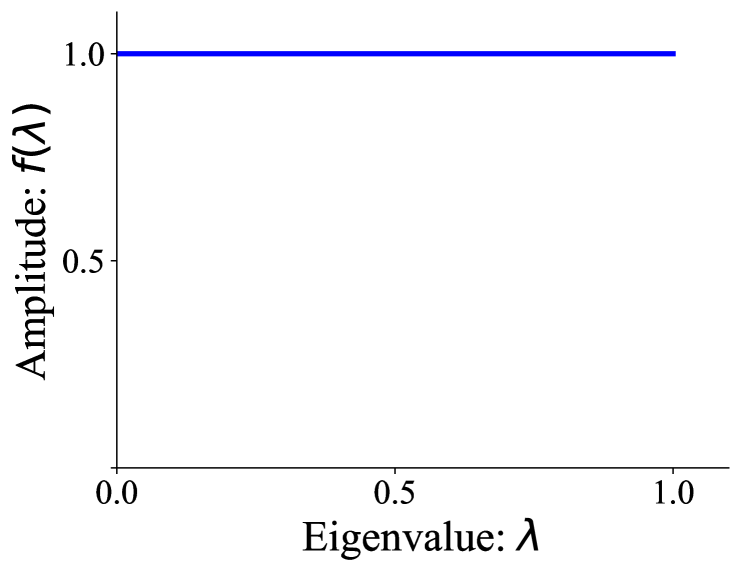
(a) All-pass, $f(\lambda)=1$

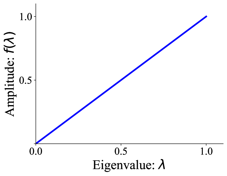
(b) Low-pass, $f(\lambda)=\lambda$

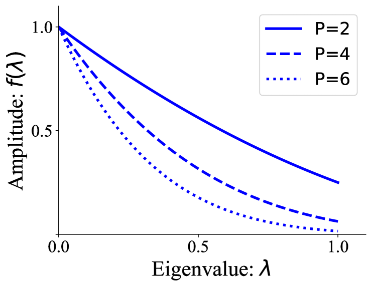
(c) High-pass, $f(\lambda)=(1-0.5\lambda)^{P}$

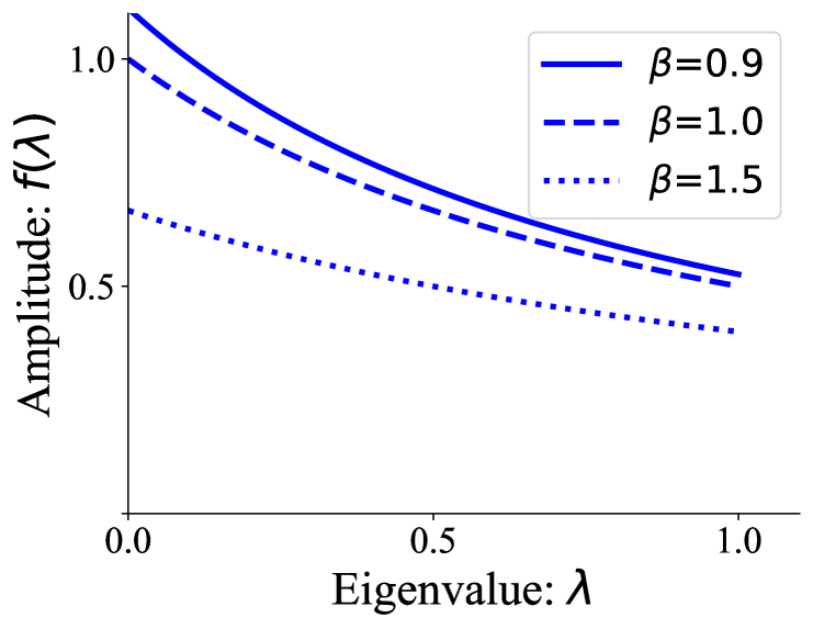
(d) High-pass, $f(\lambda)=(\lambda+\beta)^{-1}$

Figure 1: Visualization of different filtering functions. A larger eigenvalue indicates a lower frequency. If $f(\lambda)$ has a large value when $\lambda$ is small, then $f(\cdot)$ is a high-pass filter, and vice versa.

(a) Raw image

(b) Low-pass

(c) $\beta=0.1$

(d) $\beta=0.01$

Figure 2: Synthetic images distilled by different filters.

The above analysis emphasizes that the design of filter functions $f(\cdot)$ plays a vital role in DD. Therefore, this section further analyzes the differences between filters, including all-pass, low-pass, and high-pass. See Figure 1 for the visualizations of different filters.

The all-pass filter maps all eigenvalues to 1 and maintains all frequency information of the input signal. Although there is no information loss, the filter will make the synthetic dataset converge to a trivial solution, i.e., $X_{s}^{\top}X_{s}=I$, which cannot encode the knowledge of the real dataset, i.e., $X^{\top}X$.

Low-pass filters amplify the impact of low-frequency information, which represents the global texture of natural images. Similarly, we find that matching the low-frequency information of the FFC matrix enables synthetic images to learn the texture of the real dataset. Figure 2(a) is a raw goldfish image in Tiny-ImageNet. When applying a low-pass filter on the FFC matrix, the synthetic image, shown in Figure 2(b), becomes blurred.

In contrast, high-pass filters emphasize the local fine-grained details of the input data. Figures 2(c) and 2(d) illustrates the synthetic images learned by the high-pass filter $f(\lambda)=(\lambda+\beta)^{-1}$ with different hyper-parameters. The results demonstrate that smaller values of $\beta$ allow the synthesized images to capture more intricate details. Thus, by tuning the value of $\beta$, we can modulate the frequency distribution within the synthetic images.

3 The Proposed Method

Both low- and high-frequency features contribute to the training of neural networks [Frequency]. It is intuitive to preserve both information in the synthetic datasets. However, existing DD methods only have fixed filter functions and cannot capture the diverse frequency information of the real datasets, which motivates the design of our model.

Curriculum Frequency Matching

For the high-pass filter $f(\lambda)=(\lambda+\beta)^{-1}$, we can control its shape by adjusting the value of $\beta$. As the value of $\beta$ increases from zero, the proportion of low-frequency information gradually increases. When $\beta$ approaches infinity, the high-pass filter will degenerate into the all-pass filter. Therefore, we propose to assign different values of $\beta$ during distillation to enhance the diversity of the synthetic datasets. Specifically, we use a pre-defined scheduler to control the change of $\beta$, defined as:

$$\beta_{t}=\beta*(1+\cos(\pi t/T))/2,$$ (16)

where $\beta$ is a hyper-parameter to control the frequency band, $t$ indicates the current step, and $T$ is the maximum step.

Implement of FFC and FLC.

Advanced methods [SRe2L, G-VBSM, D3S] suggest matching the representations of real and synthetic datasets in each layer of the backbone network, rather than just matching the last layer. Following this principle, CFM calculates the FFC and FLC matrices based on the input data in each layer, which is a feature map $X$ with shape $n\times d\times h\times w$, indicating the number of images, channel, height, and weight, respectively. For the FFC matrix, we reshape the feature map into channel-level representations, and for the FLC matrix, we average the height and weight dimensions of $X$:

$$\hat{X}=\text{reshape}(X)\in\mathbb{R}^{nhw\times d},\quad X^{\prime}=\text{avg}(X)\in\mathbb{R}^{n\times d}.$$ (17)

In practice, directly computing $\hat{X}^{\top}\hat{X}$ suffers from numerical overflow problems because the reshape operator significantly increases the number of samples from $n$ to $nhw$. Therefore, we use the covariance of $\hat{X}^{\top}\hat{X}$ and the average of ${X^{\prime}}^{\top}Y$ as substitutes for FFC and FLC to stabilize the training process of CFM:

$$\Psi=\frac{1}{nhw}(\hat{X}-\bar{X})^{\top}(\hat{X}-\bar{X}),\quad\Phi=\frac{1}{n}{X^{\prime}}^{\top}Y,$$ (18)

where $\Psi$ and $\Phi$ denote the normalized FFC and FLC matrices, and $\bar{X}$ is the average of $\hat{X}$.

Exponential Moving Updating (EMU).

The computation of $\Psi$ and $\Phi$ is affordable for real datasets but is much more complex for synthetic datasets. In practice, we can only calculate $\Psi_{s}$ and $\Phi_{s}$ in a mini-batch manner, which differs from the full-batch assumption in the theoretical analysis. To mitigate this gap, we adopt a moving update technology [G-VBSM, D3S] to cache the result of each batch and ultimately approximate the statistics of the real datasets:

$$\Psi_{s}=\frac{1}{b}\Psi_{s}^{b}+(1-\frac{1}{b})\Psi_{s}^{b-1},\quad\Phi_{s}=\frac{1}{b}\Phi_{s}^{b}+(1-\frac{1}{b})\Phi_{s}^{b-1},$$ (19)

where $\Psi_{s}^{b}$ and $\Psi_{s}^{b-1}$ indicate the FFC matrices of the current $b$-th batch and the previous batch, respectively. The symbols of the FLC matrices are the same as above.

Final Loss Function.

Recalling the analysis in Section 2, the filter functions $f$ of different methods vary differently, but the choice of $g$ is limited to $g(X^{\top}Y)=I$ or $X^{\top}Y$. The former corresponds to a filter-matching loss, while the latter leads to a signal-matching loss. In the context of CFM, we define the loss functions as:

$$\mathcal{L}_{\text{filter}} =\sum_{l=1}^{L}\left\|(\Psi^{l}+\beta_{t}I)^{-1}-(\Psi_{s}^{l}+\beta_{t}I)^{-1}\right\|,$$ (20)

$$\mathcal{L}_{\text{signal}} =\sum_{l=1}^{L}\left\|(\Psi^{l}+\beta_{t}I)^{-1}\Phi^{l}-(\Psi_{s}^{l}+\beta_{t}I)^{-1}\Phi_{s}^{l}\right\|,$$

where $l$ is the layer index of the distillation network. By combining these two functions with the traditional classification loss, we get the final loss function:

$$\mathcal{L}=\mathcal{L}_{\text{cls}}(H_{s},Y_{s})+\eta\mathcal{L}_{\text{filter}}+\eta\mathcal{L}_{\text{signal}}$$ (21)

where $\eta=0.1$ is a hyperparameter for all datasets for simplicity. An overview of CFM is shown in Algorithm 1.

Algorithm 1 Curriculum Frequency Matching

1:Distillation network $\phi$, real dataset $\mathcal{T}=(H,Y)$, minimum parameter $\beta_{\min}$, maximum step $T$, number of iteration $\mathcal{I}$, batch size $|B|$.

2:Synthetic dataset $\mathcal{S}=(H_{s},Y_{s})$

3:Feed $H$ into $\phi$ for a forward pass

4:for layer index $l=1,\cdots,L$ do

5:  Calculate $\Psi^{l}$ and $\Phi^{l}$ based on Eq. 18

6:end for

7:for batch index $b=1,\cdots,\frac{m}{|B|}$ do

8:  Initialize $H_{s}^{b}$ with randomly sampled real data

9:  Update $\beta_{t}$ based on Eq. 16

10:  repeat

11:   Feed $H_{s}^{b}$ into $\phi$ for a forward pass

12:   for layer index $l=1,\cdots,L$ do

13:     Calculate $\Psi_{s}^{l}$ and $\Phi_{s}^{l}$ based on Eq. 19

14:     Calculate $\mathcal{L}_{\text{filter}}$ and $\mathcal{L}_{\text{signal}}$ based on Eq. 20

15:   end for

16:   Calculate $\mathcal{L}_{\text{ce}}$ and back-propagate $\mathcal{L}$

17:   Update $H_{s}^{b}$

18:  until Reached the number of iteration $\mathcal{I}$

19:end for

4 Experiments

Table 2: Performance (%) of different DD methods in CIFAR-10/100. The best performance is highlighted in bold. Results are taken from the original papers, and $-$ indicates missing data.

Dataset

IPC

ConvNet-128

ResNet-18

DM

DC

MTT

KIP

G-VBSM

DWA

CFM

SRe2L

G-VBDM

DWA

CFM

CIFAR-10

10

48.9±0.6

44.9±0.5

65.3±0.7

46.1±0.7

46.5±0.7

45.0±0.4

52.1±0.5

27.2±0.5

53.5±0.6

32.6±0.4

57.0±0.3

50

63.0±0.4

53.9±0.5

71.6±0.2

53.2±0.7

54.3±0.3

63.3±0.7

64.0±0.4

47.5±0.6

59.2±0.4

53.1±0.3

82.3±0.4

CIFAR-100

10

29.7±0.3

25.2±0.3

33.1±0.4

40.1±0.4

38.7±0.2

47.6±0.4

58.3±0.4

31.6±0.5

59.5±0.4

39.6±0.6

64.6±0.4

50

43.6±0.4

30.6±0.6

42.9±0.3

$-$

45.7±0.4

59.0±0.1

67.1±0.3

49.5±0.3

65.0±0.5

60.3±0.5

71.4±0.2

Table 3: Performance (%) of different DD methods in Tiny-ImageNet and ImageNet-1k. Results are taken from the original papers and the symbol ${\dagger}$ indicates 200 epochs evaluation in Tiny-ImageNet, while others are 100 epochs.

	Dataset	Tiny-ImageNet		ImageNet-1K
	IPC	50	100	10	50	100	200
ResNet-18	SRe2L [SRe2L]	41.4±0.4	49.7±0.3	21.3±0.6	46.8±0.2	52.8±0.3	57.0±0.4
	CDA [CDA]	48.7	53.2	$-$	53.5	58.0	63.3
	G-VBSM [G-VBSM]	47.6±0.3	51.0±0.4	31.4±0.5	51.8±0.4	55.7±0.4	$-$
	DWA [DWA]†	52.8±0.2	56.0±0.2	37.9±0.2	55.2±0.2	59.2±0.3	$-$
	CFM	54.6±0.2	57.6±0.1	38.3±0.3	57.3±0.2	60.1±0.2	63.6±0.2
ResNet-50	SRe2L [SRe2L]	42.2±0.5	51.2±0.4	28.4±0.1	55.6±0.3	61.0±0.4	64.6±0.3
	CDA [CDA]	50.6	55.0	$-$	61.3	65.1	67.6
	G-VBSM [G-VBSM]	48.7±0.2	52.1±0.3	35.4±0.8	58.7±0.3	62.2±0.3	$-$
	DWA [DWA]†	53.7±0.2	56.9±0.4	43.0±0.5	62.3±0.1	65.7±0.4	$-$
	CFM	54.8±0.2	58.2±0.3	42.9±0.4	63.2±0.2	66.1±0.3	67.9±0.4
ResNet-101	SRe2L [SRe2L]	42.5±0.2	51.5±0.3	30.9±0.1	60.8±0.5	62.8±0.2	65.9±0.3
	CDA [CDA]	50.6	55.0	$-$	61.6	65.9	68.4
	G-VBSM [G-VBSM]	48.8±0.4	52.3±0.1	38.2±0.4	61.0±0.4	63.7±0.2	$-$
	DWA [DWA]†	54.7±0.3	57.4±0.3	46.9±0.4	63.3±0.7	66.7±0.2	$-$
	CFM	55.3±0.3	59.2±0.3	43.0±0.3	63.5±0.2	66.9±0.3	68.8±0.3

Table 4: Cross-architecture performance (%) of different DD methods. $\ddagger$ indicates that the results are our evaluation, otherwise, we adopt the results from the original paper. The results of DWA are not reported due to the lack of source code and synthetic images.

ImageNet-1k (IPC=50)	Validaton Model
	ResNet-18	ResNet-50	ResNet-101	DenseNet-121	RegNet-Y-8GF	ConvNeXt-Tiny
SRe2L	46.80	55.60	60.81	49.47	60.34	53.53
CDA	53.45	61.26	61.57	57.35	63.22	62.58
G-VBSM‡	51.8	58.7	61.0	58.47	62.02	61.93
CFM	57.32	63.23	63.46	60.91	64.03	64.89

In this section, we compare the proposed method with several competitive DD methods on various datasets and settings.

4.1 Experimental Setup

Datasets.

We consider four datasets, ranging from small to large scale, including CIFAR-10/100 [CIFAR] (32$\times$32, 10/100 classes), Tiny-ImageNet [Tiny] (64$\times$64, 200 classes), and ImageNet-1K [ImageNet] (224$\times$224, 1000 classes).

Networks.

Following SR²L [SRe2L], we use ResNet-18 [ResNet] as the distillation network for all datasets. For a fair comparison with traditional DD methods, we also use ConvNet-128 [DC] in CIFAR-10/100, as suggested by G-VBSM. We adopt various memory budgets for different datasets, including image per class (IPC)-10, 50, 100, and 200.

Baselines.

Traditional DD methods only worked on small-scale datasets, e.g., CIFAR-10/100, but do not perform well in large-scale datasets, e.g., ImageNet-1K. In this case, we select DM [DM], DC [DC], MTT [MTT], and KIP [KIP] as baselines in CIFAR-10/100. Moreover, we report the performance of some more recent DD methods, including SRe²L [SRe2L], CDA [CDA], G-VBSM [G-VBSM], and DWA [DWA] in all datasets.

Evaluation.

In the evaluation phase, we adopt the Fast Knowledge Distillation (FKD) strategy suggested by SRe²L, which has been proven to be useful for large-scale datasets. For a fair comparison, we strictly control the hyperparameters of FKD to be the same as previous methods. See Appendix 2.1 for more details.

4.2 Quantitative Results

We conduct experiments on both small-scale and large-scale datasets. The results are shown in Tables 2 and 3, respectively, from which we have the following observations:

CIFAR-10/100.

Traditional DD methods perform well on datasets with fewer classes, i.e., CIFAR-10, and shallow models, i.e., ConvNet-128. The advanced DD methods are more effective when the dataset becomes larger and the network goes deeper. We can observe that CFM consistently outperforms all advanced DD methods by a large margin. Notably, ResNet-18 trained on the original datasets has an accuracy of 94.25% and 77.45% on CIFAR-10/100. The performance of existing methods is far from achieving optimal results, while CFM is significantly approaching, demonstrating its effectiveness in distilling low-resolution data.

Tiny-ImageNet & ImageNet-1k.

In the large-scale datasets, we use ResNet-{18, 50, 101} to evaluate the performance of different methods. In the Tiny-ImageNet part, we can find that CFM has an average of 3% performance improvement over DWA, which is the most recent method using advanced model augmentation strategies. This indicates that CFM is highly competitive with state-of-the-art methods. In the ImageNet-1k part, we can see that CFM consistently surpasses all baselines in IPC=50, 100, and 200, validating its superiority over the advanced DD methods. Moreover, we observe that DWA performs better than CFM in IPC=10. We suspect that this is because the synthetic data cannot effectively cover the useful frequency features under the limited memory budget, leading to the performance degeneration of CFM.

4.3 Cross-architecture Generalization

In addition to classification accuracy, cross-architecture generalization is also crucial for DD. Ideally, synthetic datasets should encode the knowledge of real datasets rather than over-fitting to a specific model architecture. Therefore, we use diverse networks, including ResNet-50/101, DenseNet-121 [densenet], RegNet-Y-8GF [regnet], and ConvNeXt-Tiny [convnext], to evaluate the generalization ability of different DD methods on the ImageNet-1k dataset with IPC=50. The distillation network is uniformly set to ResNet-18. Results are shown in Table 4, from which we can see that CFM achieves the best performance by a substantial margin across different architectures. We speculate that the high-frequency information is transferable across different architectures. Therefore, CFM encodes the architecture-invariant knowledge of the real datasets and exhibits powerful cross-architecture generalization ability.

Table 5: Ablation studies on the loss functions of CFM. Experiments are conducted on datasets with IPC=50.

Loss Functions			Datasets
$\mathcal{L}_{\text{filter}}$	$\mathcal{L}_{\text{signal}}$	$\mathcal{L}_{\text{cls}}$	CIFAR-100	Tiny	ImageNet
✓			64.95	51.20	53.43
✓	✓		67.32	51.92	55.76
✓	✓	✓	72.48	54.84	57.32

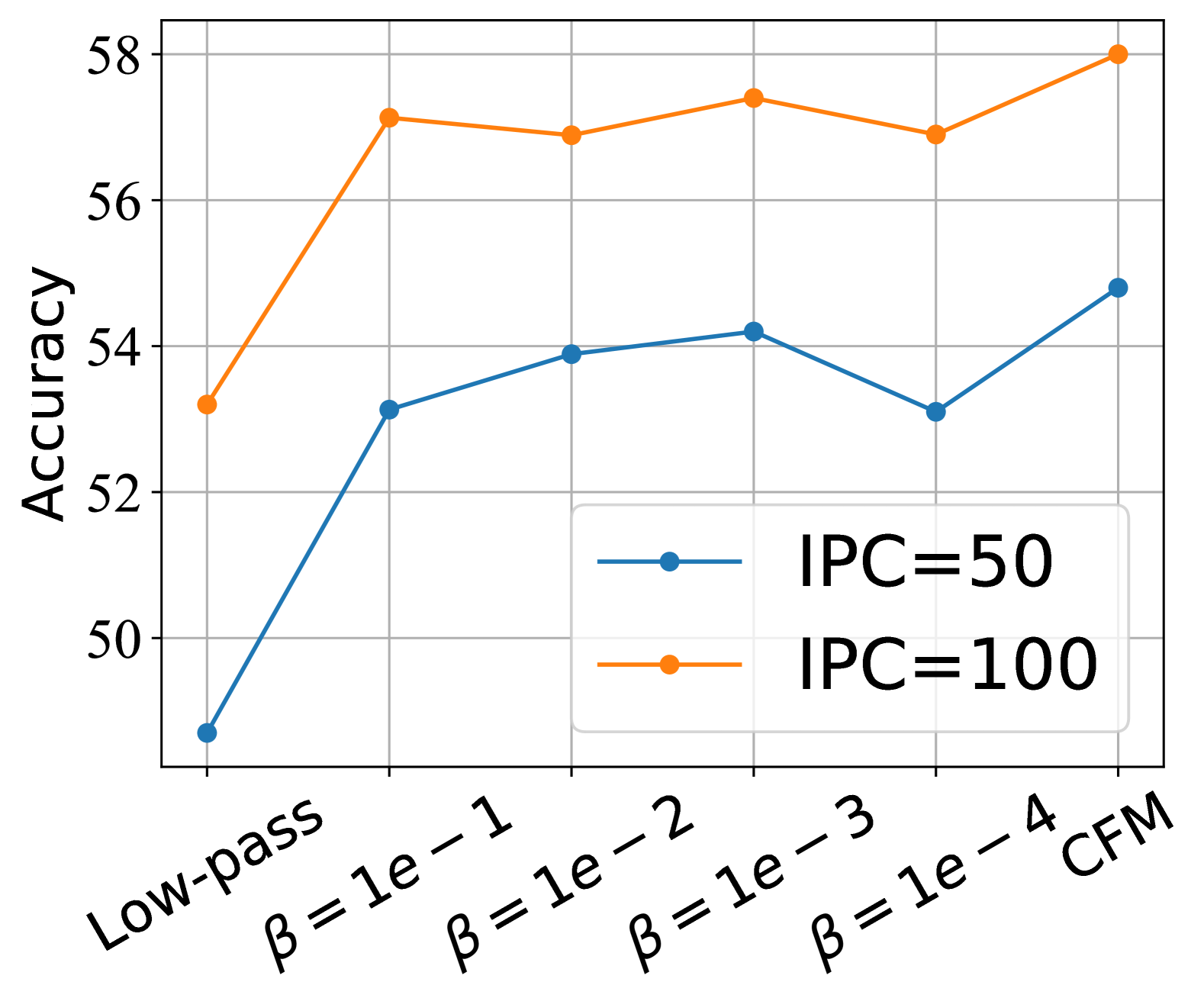
(a) Tiny-ImageNet

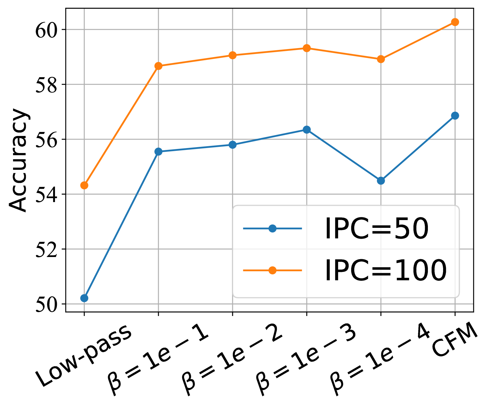
(b) ImageNet-1k

Figure 3: Ablation studies on the choice of filters.

4.4 Ablation Studies

We conducted two experiments to demonstrate the importance of each module in the proposed model. The first experiment, shown in Table 5, is used to identify the effectiveness of different loss functions. Specifically, we sequentially remove the classification loss, i.e., $\mathcal{L}_{\text{cls}}$ and signal-matching loss, i.e., $\mathcal{L}_{\text{signal}}$, and evaluate CFM on three datasets, including CIFAR-100, Tiny-ImageNet, and ImageNet-1k. We can observe that all three loss functions contribute to the performance of CFM, and the filter-matching loss plays a fundamental role. This discovery suggests that the important knowledge of the real datasets may encoded in the FFC matrix of the feature maps.

The second experiment is used to verify the effectiveness of the curriculum strategy. Specifically, we evaluate the performance of different filters, including low-pass filter, high-pass filter with parameter $\beta=1e^{-1},1e^{-2},1e^{-3},1e^{-4}$, and high-pass filter with CFM. The results are shown in Figure 3, from which we can find that the performance of the low-pass filter is far away from the high-pass filters, indicating that the high-frequency information is more important for DD. However, the extremely high frequency will also lead to performance degradation. For example, the performance of $\beta=1e^{-4}$ is not as good as other parameters. On the other hand, CFM balances the proportion between low-frequency and high-frequency information by setting a proper frequency band, consistently outperforming other filters.

	Tiny-ImageNet			ImageNet-1k
SRe2L
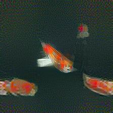
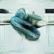
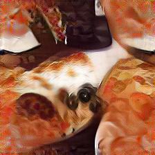
G-VBSM
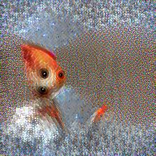
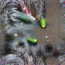
CFM
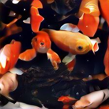
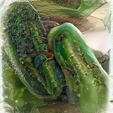
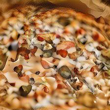
	GoldFish	Jellyfish	Snail	GoldFish	Cucumber	Pizza

Figure 4: Visualization of the images synthesized by different DD methods.

4.5 Visualization

To provide a more intuitive comparison of various DD methods, we visualize the synthetic images generated by SRe²L, G-VBSM, and CFM in Figure 4. It can be observed that SRe²L and G-VBSM struggle to produce meaningful images, particularly with the low-resolution Tiny-ImageNet dataset. In contrast, the images synthesized by CFM exhibit clear semantic information, e.g., recognizable shapes, demonstrating the effectiveness of matching frequency-specific features between the real and synthetic datasets.

5 Related Work

As we have analyzed the objectives of DD in Section 2, we only introduce some orthogonal research lines, including data parameterization, model augmentation, and theory.

Data Parameterization.

Traditionally, the synthetic images are optimized in the pixel space, which is inefficient due to the potential data redundancy. Therefore, some methods explore how to parameterize the synthetic images. IDC [IDC] distillates low-resolution images to save budget and up-samples them in the evaluation stage. Haba [Haba] designs a decoder network to combine different latent codes for diverse synthetic datasets. RDED [RDED] stitches the core patches of real images together as the synthetic data. Some methods use generative models to decode the synthetic datasets from latent codes, including GAN-based methods [IT-GAN, MGDD] and diffusion-based methods [diff1, diff2]. Generally, data parameterization can be incorporated with different DD objectives to reduce their storage budgets and improve efficiency.

Model Augmentation.

The knowledge of the datasets is mostly encoded in the pre-train distillation networks. Therefore, some methods focus on training a suitable network for DD by designing some augmentation strategies. FTD [FTD] constrains model weights to achieve a flat trajectory and reduces the accumulated errors in MTT. model_aug uses early-stage models and parameter perturbation to increase the search space of the parameters. More recently, DWA [DWA] employs directed weight perturbations on the pre-train models, which not only maintains the unique features of each synthetic data but also improves the diversity.

Theory.

Some works tend to explore DD from a theoretical perspective. For example, theorem_size analyzes the size and approximation error of the synthetic datasets. theorem_bias explores the influence of spurious correlations in DD. theorem_learning explains the information captured by the synthetic datasets. theorem_core provides a formal definition of DD and provides a foundation analysis on the optimization of DD. Although these methods have some important insights, they fail to explain the roles of existing methods. In contrast, UniDD establishes the relationship between DD objectives and spectral filtering.

6 Conclusion

In this paper, we introduce UniDD, a framework that unifies various DD objectives through spectral filtering. UniDD demonstrates that each DD objective corresponds to a filter function applied on the FFC and FLC matrices. This finding reveals the nature of various DD methods and inspires the design of new methods. Based on UniDD, we propose CFM to encode both low- and high-frequency information by gradually changing the filter parameter. Experiments conducted on various datasets validate the effectiveness and generalization of the proposed method. A promising future direction is to generalize UniDD to the distillation of unsupervised and multi-modal datasets.

Supplementary Material

1 Derivation of UniDD

The derivation of statistical matching, gradient matching, and trajectory matching is relatively intuitive and has been fully introduced in the main text. Here, we mainly derive the conclusion of KRR, which is closely related to the proposed model. Generally, the objective of KRR is defined as:

$$\mathcal{L}_{KRR}=||\mathcal{K}W-Y||_{F}^{2}+\beta W^{\top}\mathcal{K}W,$$ (1)

where $\mathcal{K}\in\mathbb{R}^{n\times n}$ is the Gram matrix of input data.

By taking the derivative with respect to $W$, we have:

$$\nabla_{W}=\mathcal{K}^{\top}(\mathcal{K}W-Y)+\beta(\mathcal{K}W+\mathcal{K}^{\top}W).$$ (2)

When set the gradient to zero, we have:

$$W^{*}=(\mathcal{K}+\beta I)^{-1}Y.$$ (3)

This equation gives an optimal solution of $W$, which can be used to replace the inner loop of DD. If implemented with the linear kernel, we have:

$$W_{s}=(X_{s}X_{s}^{\top}+\beta I)^{-1}Y_{s}.$$ (4)

The outer loop of DD treats $W_{s}$ a classifier to minimize the classification error in the real datasets:

$$\left\|Y-\mathcal{K}_{ts}W_{s}\right\|^{2}=\left\|Y-XX_{s}^{\top}(X_{s}X_{s}^{\top}+\beta I)^{-1}Y_{s}\right\|_{F}^{2},$$ (5)

which derivatives Equation 12 in the main text.

Another detail is the identity transformation, formulated as

$$\mathbf{P}(\mathbf{Q}\mathbf{P}+\mathbf{I})^{-1}=(\mathbf{PQ}+\mathbf{I})^{-1}\mathbf{P}.$$ (6)

By setting $X_{s}^{\top}=\mathbf{P}$ and $X_{s}=\mathbf{Q}$, we have:

$$X_{s}^{\top}(X_{s}X_{s}^{\top}+\beta I)^{-1}=(X_{s}^{\top}X_{s}+\beta I)^{-1}X_{s}^{\top}.$$ (7)

Based on this equation, we successfully transform the Gram matrix into the FFC matrix and unify KRR-based methods into UniDD.

2 Implementation Details.

2.1 Experimental Setup

We use the squeeze, recover, and relabel pipeline, introduced by SRe²L, for the distillation of CFM. The details of datasets, setup (e.g., optimizer), and hyper-parameters are listed in Tables 1, 2, 3, and 4.

Table 1: Statistics of datasets.

	CIFAR-10	CIFAR-100	Tiny-ImageNet	ImageNet-1k
Classes	10	100	200	1000
Training	50,000	50,000	100,000	1,281,167
Validation	10,000	10,000	10,000	50,000
Resolution	64$\times$64	64$\times$64	64$\times$64	224$\times$224

Table 2: Squeeze Configurations of CFM.

Config	CIFAR-10/100	Tiny-ImageNet	ImageNet-1k
Epoch	200 / 100	50	90
Optimizer	SGD	SGD	SGD
Learning Rate	0.1	0.2	0.1
Momentum	0.9	0.9	0.9
WeightDecay	5e-4	1e-4	1e-4
BatchSize	128	256	256
Scheduler	Cosine	Cosine	Step (0.1 / 30 epochs)
Augmentation	RandomCrop HorizontalFlip	RandomResizedCrop HorizontalFlip	RandomResizedCrop HorizontalFlip

Table 3: Recover Configurations of CFM.

Config	CIFAR-10/100	Tiny-ImageNet	ImageNet-1k
$\beta$	0.1	1.0	0.1
Iteration	1000	1000	1000
Optimizer	Adam	Adam	Adam
Learning Rate	0.25	0.1	0.1
Betas	(0.5, 0.9)	(0.5, 0.9)	(0.5, 0.9)
BatchSize	10/100	200	500
Scheduler	Cosine	Cosine	Cosine
Augmentation	RandomResizedCrop HorizontalFlip	RandomResizedCrop HorizontalFlip	RandomResizedCrop HorizontalFlip

Table 4: Recover & Validation Configurations of CFM.

Config	CIFAR-10/100	Tiny-ImageNet	ImageNet-1k
Epoch	1000	100	300
Optimizer	Adam / SGD	SGD	Adam
Learning Rate	1e-3 / 1e-1	2e-1	1e-3
Parameters	- / Mom=0.9	Mom=0.9	-
WeightDecay	5e-4	1e-4	1e-4
BatchSize	64	64	128
Scheduler	Cosine	Cosine	Cosine
Temperature	30	20	20
Augmentation	RandomCrop HorizontalFlip	RandomResizedCrop HorizontalFlip	RandomResizedCrop HorizontalFlip

3 Visualization

Finally, we visualize the synthetic images of ImageNet-1k to provide a comprehensive exhibition.

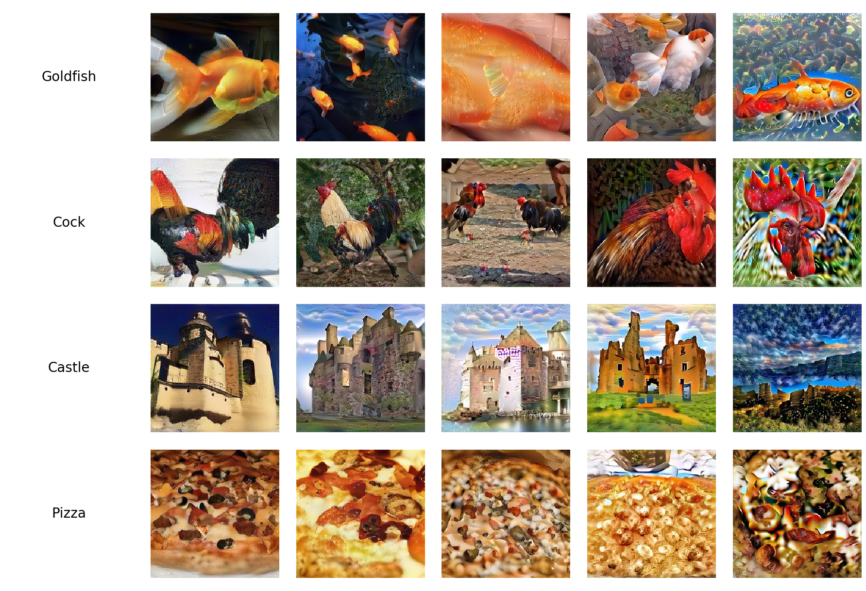
Figure 5: Synthetic images of ImageNet-1k. From left to right, the frequency gradually increases.

References

- Arveson [2002] William Arveson. A short course on spectral theory. Springer, 2002.
- Cazenavette et al. [2022] George Cazenavette, Tongzhou Wang, Antonio Torralba, Alexei A. Efros, and Jun-Yan Zhu. Dataset distillation by matching training trajectories. In CVPR, pages 10708–10717. IEEE, 2022.
- Cui et al. [2023] Justin Cui, Ruochen Wang, Si Si, and Cho-Jui Hsieh. Scaling up dataset distillation to imagenet-1k with constant memory. In ICML, pages 6565–6590. PMLR, 2023.
- Cui et al. [2024] Justin Cui, Ruochen Wang, Yuanhao Xiong, and Cho-Jui Hsieh. Ameliorate spurious correlations in dataset condensation. In ICML. OpenReview.net, 2024.
- Deng et al. [2009] Jia Deng, Wei Dong, Richard Socher, Li-Jia Li, Kai Li, and Li Fei-Fei. Imagenet: A large-scale hierarchical image database. In CVPR, pages 248–255. IEEE Computer Society, 2009.
- Deng et al. [2024] Wenxiao Deng, Wenbin Li, Tianyu Ding, Lei Wang, Hongguang Zhang, Kuihua Huang, Jing Huo, and Yang Gao. Exploiting inter-sample and inter-feature relations in dataset distillation. In CVPR. IEEE, 2024.
- Ding et al. [2024] Jianrong Ding, Zhanyu Liu, Guanjie Zheng, Haiming Jin, and Linghe Kong. Condtsf: One-line plugin of dataset condensation for time series forecasting. In NeurIPS, 2024.
- Dosovitskiy et al. [2021] Alexey Dosovitskiy, Lucas Beyer, Alexander Kolesnikov, Dirk Weissenborn, Xiaohua Zhai, Thomas Unterthiner, Mostafa Dehghani, Matthias Minderer, Georg Heigold, Sylvain Gelly, Jakob Uszkoreit, and Neil Houlsby. An image is worth 16x16 words: Transformers for image recognition at scale. In ICLR. OpenReview.net, 2021.
- Du et al. [2023] Jiawei Du, Yidi Jiang, Vincent Y. F. Tan, Joey Tianyi Zhou, and Haizhou Li. Minimizing the accumulated trajectory error to improve dataset distillation. In CVPR, pages 3749–3758. IEEE, 2023.
- Du et al. [2024] Jiawei Du, Xin Zhang, Juncheng Hu, Wenxing Huang, and Joey Tianyi Zhou. Diversity-driven synthesis: Enhancing dataset distillation through directed weight adjustment. In NeurIPS, 2024.
- Geng et al. [2023] Jiahui Geng, Zongxiong Chen, Yuandou Wang, Herbert Woisetschlaeger, Sonja Schimmler, Ruben Mayer, Zhiming Zhao, and Chunming Rong. A survey on dataset distillation: Approaches, applications and future directions. In IJCAI, pages 6610–6618. ijcai.org, 2023.
- Gu et al. [2024] Jianyang Gu, Saeed Vahidian, Vyacheslav Kungurtsev, Haonan Wang, Wei Jiang, Yang You, and Yiran Chen. Efficient dataset distillation via minimax diffusion. In CVPR, pages 15793–15803. IEEE, 2024.
- Guo et al. [2024] Ziyao Guo, Kai Wang, George Cazenavette, Hui Li, Kaipeng Zhang, and Yang You. Towards lossless dataset distillation via difficulty-aligned trajectory matching. In ICLR. OpenReview.net, 2024.
- He et al. [2016] Kaiming He, Xiangyu Zhang, Shaoqing Ren, and Jian Sun. Deep residual learning for image recognition. In CVPR, pages 770–778. IEEE Computer Society, 2016.
- Huang et al. [2017] Gao Huang, Zhuang Liu, Laurens van der Maaten, and Kilian Q. Weinberger. Densely connected convolutional networks. In CVPR, pages 2261–2269. IEEE Computer Society, 2017.
- Jin et al. [2022] Wei Jin, Lingxiao Zhao, Shichang Zhang, Yozen Liu, Jiliang Tang, and Neil Shah. Graph condensation for graph neural networks. In ICLR. OpenReview.net, 2022.
- Kim et al. [2022] Jang-Hyun Kim, Jinuk Kim, Seong Joon Oh, Sangdoo Yun, Hwanjun Song, Joonhyun Jeong, Jung-Woo Ha, and Hyun Oh Song. Dataset condensation via efficient synthetic-data parameterization. In ICML, pages 11102–11118. PMLR, 2022.
- Kirillov et al. [2023] Alexander Kirillov, Eric Mintun, Nikhila Ravi, Hanzi Mao, Chloé Rolland, Laura Gustafson, Tete Xiao, Spencer Whitehead, Alexander C. Berg, Wan-Yen Lo, Piotr Dollár, and Ross B. Girshick. Segment anything. In ICCV, pages 3992–4003. IEEE, 2023.
- Krizhevsky et al. [2009] Alex Krizhevsky, Geoffrey Hinton, and et al. Learning multiple layers of features from tiny images. 2009.
- Kungurtsev et al. [2024] Vyacheslav Kungurtsev, Yuanfang Peng, Jianyang Gu, Saeed Vahidian, Anthony Quinn, Fadwa Idlahcen, and Yiran Chen. Dataset distillation from first principles: Integrating core information extraction and purposeful learning. CoRR, abs/2409.01410, 2024.
- Le and Yang [2015] Ya Le and Xuan Yang. Tiny imagenet visual recognition challenge. CS 231N, 7(7):3, 2015.
- Lei and Tao [2024] Shiye Lei and Dacheng Tao. A comprehensive survey of dataset distillation. IEEE Trans. Pattern Anal. Mach. Intell., 46(1):17–32, 2024.
- Liu and Wang [2023] Songhua Liu and Xinchao Wang. MGDD: A meta generator for fast dataset distillation. In NeurIPS, 2023.
- Liu et al. [2022a] Songhua Liu, Kai Wang, Xingyi Yang, Jingwen Ye, and Xinchao Wang. Dataset distillation via factorization. In NeurIPS, 2022a.
- Liu et al. [2024a] Yang Liu, Deyu Bo, and Chuan Shi. Graph distillation with eigenbasis matching. In ICML. OpenReview.net, 2024a.
- Liu et al. [2022b] Zhuang Liu, Hanzi Mao, Chao-Yuan Wu, Christoph Feichtenhofer, Trevor Darrell, and Saining Xie. A convnet for the 2020s. In CVPR, pages 11966–11976. IEEE, 2022b.
- Liu et al. [2024b] Zhanyu Liu, Ke Hao, Guanjie Zheng, and Yanwei Yu. Dataset condensation for time series classification via dual domain matching. In KDD, pages 1980–1991. ACM, 2024b.
- Loo et al. [2022] Noel Loo, Ramin M. Hasani, Alexander Amini, and Daniela Rus. Efficient dataset distillation using random feature approximation. In NeurIPS, 2022.
- Loo et al. [2024] Noel Loo, Alaa Maalouf, Ramin M. Hasani, Mathias Lechner, Alexander Amini, and Daniela Rus. Large scale dataset distillation with domain shift. In ICML. OpenReview.net, 2024.
- Maalouf et al. [2023] Alaa Maalouf, Murad Tukan, Noel Loo, Ramin M. Hasani, Mathias Lechner, and Daniela Rus. On the size and approximation error of distilled sets. In NeurIPS. OpenReview.net, 2023.
- Nguyen et al. [2021] Timothy Nguyen, Zhourong Chen, and Jaehoon Lee. Dataset meta-learning from kernel ridge-regression. In ICLR. OpenReview.net, 2021.
- Radford et al. [2021] Alec Radford, Jong Wook Kim, Chris Hallacy, Aditya Ramesh, Gabriel Goh, Sandhini Agarwal, Girish Sastry, Amanda Askell, Pamela Mishkin, Jack Clark, Gretchen Krueger, and Ilya Sutskever. Learning transferable visual models from natural language supervision. In ICML, pages 8748–8763. PMLR, 2021.
- Sachdeva and McAuley [2023] Noveen Sachdeva and Julian J. McAuley. Data distillation: A survey. CoRR, abs/2301.04272, 2023.
- Shao et al. [2024] Shitong Shao, Zeyuan Yin, Muxin Zhou, Xindong Zhang, and Zhiqiang Shen. Generalized large-scale data condensation via various backbone and statistical matching. In CVPR, pages 16709–16718. IEEE, 2024.
- Su et al. [2024] Duo Su, Junjie Hou, Weizhi Gao, Yingjie Tian, and Bowen Tang. Dm: Dataset distillation via disentangled diffusion model. In CVPR, pages 5809–5818. IEEE, 2024.
- Sun et al. [2024] Peng Sun, Bei Shi, Daiwei Yu, and Tao Lin. On the diversity and realism of distilled dataset: An efficient dataset distillation paradigm. In CVPR, pages 9390–9399. IEEE, 2024.
- Wang et al. [2022] Kai Wang, Bo Zhao, Xiangyu Peng, Zheng Zhu, Shuo Yang, Shuo Wang, Guan Huang, Hakan Bilen, Xinchao Wang, and Yang You. CAFE: learning to condense dataset by aligning features. In CVPR, pages 12186–12195. IEEE, 2022.
- Wang et al. [2018] Tongzhou Wang, Jun-Yan Zhu, Antonio Torralba, and Alexei A. Efros. Dataset distillation. CoRR, abs/1811.10959, 2018.
- Welling [2013] Max Welling. Kernel ridge regression. Max Welling’s classnotes in machine learning, pages 1–3, 2013.
- Xu et al. [2023] Jing Xu, Yu Pan, Xinglin Pan, Steven C. H. Hoi, Zhang Yi, and Zenglin Xu. Regnet: Self-regulated network for image classification. IEEE Trans. Neural Networks Learn. Syst., 34(11):9562–9567, 2023.
- Xu et al. [2019] Zhi-Qin John Xu, Yaoyu Zhang, Tao Luo, Yanyang Xiao, and Zheng Ma. Frequency principle: Fourier analysis sheds light on deep neural networks. CoRR, abs/1901.06523, 2019.
- Yang et al. [2023] Beining Yang, Kai Wang, Qingyun Sun, Cheng Ji, Xingcheng Fu, Hao Tang, Yang You, and Jianxin Li. Does graph distillation see like vision dataset counterpart? In NeurIPS, 2023.
- Yang et al. [2024] William Yang, Ye Zhu, Zhiwei Deng, and Olga Russakovsky. What is dataset distillation learning? In ICML. OpenReview.net, 2024.
- Yin and Shen [2023] Zeyuan Yin and Zhiqiang Shen. Dataset distillation in large data era. CoRR, abs/2311.18838, 2023.
- Yin et al. [2023] Zeyuan Yin, Eric P. Xing, and Zhiqiang Shen. Squeeze, recover and relabel: Dataset condensation at imagenet scale from A new perspective. In NeurIPS, 2023.
- Yu et al. [2024] Ruonan Yu, Songhua Liu, and Xinchao Wang. Dataset distillation: A comprehensive review. IEEE Trans. Pattern Anal. Mach. Intell., 46(1):150–170, 2024.
- Zhang et al. [2023] Lei Zhang, Jie Zhang, Bowen Lei, Subhabrata Mukherjee, Xiang Pan, Bo Zhao, Caiwen Ding, Yao Li, and Dongkuan Xu. Accelerating dataset distillation via model augmentation. In CVPR, pages 11950–11959. IEEE, 2023.
- Zhao and Bilen [2021] Bo Zhao and Hakan Bilen. Dataset condensation with differentiable siamese augmentation. In ICML, pages 12674–12685. PMLR, 2021.
- Zhao and Bilen [2022] Bo Zhao and Hakan Bilen. Synthesizing informative training samples with GAN. CoRR, abs/2204.07513, 2022.
- Zhao and Bilen [2023] Bo Zhao and Hakan Bilen. Dataset condensation with distribution matching. In WACV, pages 6503–6512. IEEE, 2023.
- Zhao et al. [2021] Bo Zhao, Konda Reddy Mopuri, and Hakan Bilen. Dataset condensation with gradient matching. In ICLR. OpenReview.net, 2021.
- Zhao et al. [2023] Ganlong Zhao, Guanbin Li, Yipeng Qin, and Yizhou Yu. Improved distribution matching for dataset condensation. In CVPR, pages 7856–7865. IEEE, 2023.
- Zhou et al. [2022] Yongchao Zhou, Ehsan Nezhadarya, and Jimmy Ba. Dataset distillation using neural feature regression. In NeurIPS, 2022.