Experimentally achieving minimal dissipation
via thermodynamically optimal transport
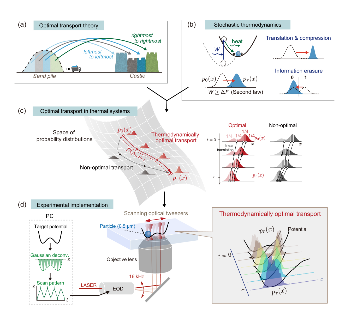
Optimal transport theory, originally developed in the 18th century for civil engineeringMonge1781, Villani2009, has since become a powerful optimization framework across disciplines, from generative AIArjovsky2017, lipman2023flow to cell biologySchiebinger2019. In physics, it has recently been shown to set fundamental bounds on thermodynamic dissipation in finite-time processesAurell2012, Nakazato2021. This extends beyond the conventional second law, which guarantees zero dissipation only in the quasi-static limit and cannot characterize the inevitable dissipation in finite-time processes. Here, we experimentally realize thermodynamically optimal transport using optically trapped microparticles, achieving minimal dissipation within a finite time. As an application to information processing, we implement the optimal finite-time protocol for information erasureAurell2012, Proesmans2020, Proesmans_2020-2, confirming that the excess dissipation beyond the Landauer boundLandauer1961, Parrondo2015 is exactly determined by the Wasserstein distance — a fundamental geometric quantity in optimal transport theory. Furthermore, our experiment achieves the bound governing the trade-off between speed, dissipation, and accuracy in information erasure. To enable precise control of microparticles, we develop scanning optical tweezers capable of generating arbitrary potential profiles. Our work establishes an experimental approach for optimizing stochastic thermodynamic processes. Since minimizing dissipation directly reduces energy consumption, these results provide guiding principles for designing high-speed, low-energy information processing.
Consider the problem of transporting a pile of sand to another location (Fig. 1a). In 1781, Gaspard Monge posed a deceptively simple yet fundamental questionMonge1781: Given the initial and final shapes of the sand piles and the cost of transporting each grain between any two positions, what is the most efficient way to minimize the total cost? This question in engineering laid the foundation for optimal transport theory, which was later formalized in applied mathematics through the incorporation of probability theory. A central concept in this framework is the Wasserstein distance, which quantifies the difference between two probability distributions in terms of the minimal transportation cost required to transform one into the otherBenamou2000, Villani2009. In recent years, optimal transport theory has found applications across various disciplines, including thermodynamics. Notably, it has been shown to establish fundamental bounds on finite-time dissipation (Fig. 1b, c), where the Wasserstein distance exactly characterizes the minimal dissipation in such processesAurell2012, Aurell2011, chen2019stochastic, Nakazato2021, ito2024geometric.
Let us start with a simple scenario in which a microparticle is immersed in a thermal environment (heat bath) at temperature . Due to thermal fluctuations, the particle undergoes stochastic motion, with its state described by a time-dependent probability distribution, denoted as . Here, represents time, and is the particle’s position. Optimal transport theory provides a natural framework for optimizing the evolution of these probability distributions. Such stochastic thermodynamic systems form the foundation of modern thermodynamics — often referred to as stochastic thermodynamics — which applies not only to a microparticle but also to a wide range of experimental systems, including electric circuits and molecular motorsSeifert2012, Ciliberto2017, Pigolotti-Peliti.
The second law of thermodynamics states that the thermodynamic work must always be greater than or equal to the nonequilibrium free-energy change Parrondo2015, which implies that the dissipated work, defined as , satisfies . This thermodynamic dissipation, which is equivalent to the entropy production multiplied by , vanishes only in the quasi-static limit requiring an infinitely long operation time. In finite-time processes, however, remains strictly positive due to unavoidable dissipation Shiraishi2016. Optimal transport theory refines the second law by providing a universal bound on finite-time dissipation:
| (1) |
where the equality is achievable for any given duration Aurell2012, Nakazato2021. Here, represents the Wasserstein distance, which is determined solely by the initial and final probability distributions at times and , denoted as and . is the particle’s friction coefficient. A key feature of is its inverse proportionality to : the greater the speed is (i.e., the shorter the operation time is), the greater the additional dissipation is. In terms of geometry, the thermodynamically optimal transport that minimizes dissipation is realized by transport along a geodesic connecting and with a uniform velocity, as illustrated in Fig. 1c (left) Villani2009, Benamou2000.
A particularly important application of the second law of thermodynamics is in determining the fundamental energy cost of information processing Parrondo2015. For example, the Landauer bound Landauer1961, Sagawa2009, Aurell2012, Lutz2015, Proesmans2020, Proesmans_2020-2 states that erasing one bit of information from a binary symmetric memory requires a minimum work of , where is the Boltzmann constant. Since the Landauer bound is achieved only in the quasi-static limit, it is desirable to establish an achievable bound for finite time processes. This can be addressed using optimal transport theory: applying Eq. (1) to information erasure yields
| (2) |
where the additional term on the right-hand side vanishes in the limit . Finite-time bounds for information erasure and the corresponding optimal protocols have been theoretically obtained Aurell2012, Proesmans2020, Proesmans_2020-2.
Despite extensive theoretical studies on thermodynamic optimal transport, experimental validation has remained unaddressed due to the necessity of precisely controlling probability distributions. Achieving the fundamental bound in finite time requires implementing the optimal time evolution of the potential with high accuracy. For instance, in non-Gaussian transport processes such as information erasure, nonharmonic potentials must be precisely controlled. While the Landauer bound itself, in the limit , was experimentally demonstrated in 2012 using optically trapped microparticles Berut2012, and various other experiments on the thermodynamics of informationJun2014, Gavrilov2016, RibezziCrivellari2019, Dago2021, Dago2023, including implementations of Maxwell’s demons have been conducted Toyabe2010, Koski2014, the thermodynamic optimization of information processing in finite time has been experimentally challenging.
In this study, we experimentally realize optimal transport by implementing the optimal protocols that minimize thermodynamic dissipation, providing the first proof-of-concept for thermodynamically optimal transport. Our experimental platform consists of a Brownian microparticle confined in a dynamically controlled potential, serving as a prototypical thermodynamic system (Fig. 1d; see also Extended Data Fig. 1). To achieve the precise control required for optimizing distribution dynamics, we built a custom optical tweezer system capable of generating arbitrary potential profiles (within the constraints of the device) through precisely engineered laser scanning patterns (see Methods). This method is general and can be applied to a wide range of systems, including feedback control and simultaneous manipulation of multiple Brownian particles.
We first investigate a simple transport problem: the translation and compression of a Gaussian distribution. This scenario, due to its simplicity and experimental feasibility, provides a clear demonstration of optimal transport by allowing direct comparisons between optimal and non-optimal protocols. In particular, our experiment reveals the geometric structure of transport, showing that the optimal transport corresponds to uniform-speed motion along a geodesic in the space of probability distributions. Furthermore, we demonstrate that optimal transport theory provides a method to evaluate dissipated work based solely on the distribution dynamics, without requiring information of individual trajectories and potential profiles. This approach is applicable even to non-optimal protocols, and potentially to complex biological systems like molecular motors Toyabe2010PRL and cells DiTerlizzi2024.
Then, we perform the experiment on information erasure, which is the primary focus of this manuscript. To implement optimal information erasure, we dynamically vary the potential profile from an initial double-well configuration to a final single-well state, achieving the finite-time bound equivalent to Eq. (2). Our experiment directly confirms that the finite-time correction to the conventional Landauer bound is given by the Wasserstein distance.
Another crucial aspect of information processing is accuracy. Typically, increasing speed increases dissipation (and thus energetic cost) and reduces accuracy Hopfield1974, Andrieux2008, Lan2012, Barato2015, dechant2022minimum, yoshimura2023housekeeping, Vu2023, ito2024geometric, Klinger2025. Such trade-offs between energy cost, speed (i.e., ), and accuracy are commonly observed in biological systems, including sensory adaptationLan2012 and information replicationHopfield1974, Andrieux2008. In our study, using the model experimental platform, we achieve the fundamental bound of this trade-off by implementing optimal information-erasure protocols with several different values of accuracy. This demonstration reinforces the universality of such trade-off in thermodynamic information processing.
Results
We begin by implementing a translation and compression protocol — a simple yet highly controllable process — to experimentally demonstrate and characterize optimal transport. Next, we realize the optimal transport for information erasure, marking the first experimental demonstration of finite-time thermodynamically optimal information processing. To accurately measure probability distributions and quantify physical quantities such as work, we perform extensive repetitions of each protocol, typically exceeding 12,000 repetitions, involving at least three different particles per condition (see Methods).
Optimal translation-compression transport in finite time
Let and be Gaussian distributions with different means and standard deviations . The Gaussian dynamics enable a detailed quantitative analysis of the transport process. To characterize optimal transport, we implement three distinct protocols: optimal, naive, and gearshift.
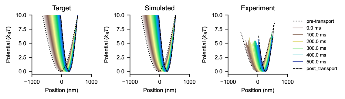
We first constructed the optimal protocol for given and (Fig. 2a-d). If and are both Gaussian, the intermediate distributions under the optimal transport protocol are always Gaussian, with linearly varying and Nakazato2021 for a distance of and a compression ratio of . and are chosen to be the same as the following naive protocol. The dynamics of potential realizing the transport are obtained by numerically solving the Fokker-Planck equation (see SI Section S2.2), which is directly implemented in our experiment. is always harmonic and has a discrete forward jump of the parameters at and a backward jump at (Fig. 2a-c). The first jump compensates for the delay due to viscous relaxation, and the last jump quenches the dynamics to the final target distribution.
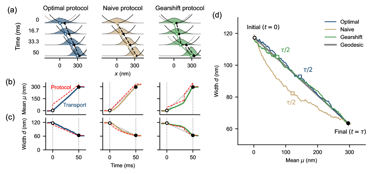
Transport can be geometrically characterized in the distribution space. We observed that the designed optimal protocol realizes the linear translation of the distribution in both and (Fig. 2a – c). Accordingly, we obtained a linear uniform-velocity trajectory in the space (Fig. 2d), where the Euclidean distance is equal to the Wasserstein distance for Gaussian distributions Villani2009. The uniform-velocity transport on a geodesic in the distribution space indicates the optimal transport Benamou2000, Nakazato2021.
The naive protocol was implemented as a reference, where the position and stiffness of a harmonic potential are linearly varied. The particle followed the potential with a time delay owing to viscous relaxation. Therefore, the final position and width of the distribution at do not reach the equilibrium values for the potential at . The trajectory in the space significantly deviated from that of the optimal protocol (Fig. 2d).
As a further reference, we also attempted a gearshift protocol, which connects two optimal protocols with different durations and speeds. This protocol realized a transport on the geodesic similarly to the optimal protocol but with a non-uniform speed (Fig. 2d). In this sense, the protocol is not optimal as a whole.
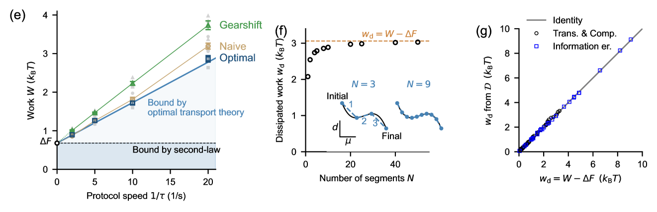
Work
The work and free energy change for transport are evaluated by using the potential , recovered from the experimental trajectories (see Methods), and the distribution (Fig. 2e). The optimal protocol achieves the theoretical minimum for finite time processes given by Eq. (1) within error bars. Accordingly, the energy-speed tradeoff was observed. was 0.680 0.007 (mean s.e.m. of all data, 48 samples). This corresponds to the compression ratio of , which is close to the designed value of 2. On the other hand, the naive protocol has larger and has a slightly nonlinear dependence on ; this implies that the transport is in the nonlinear-response regime. For a systematic comparison, we also constructed intermediate protocols by linearly interpolating optimal and naive protocols (Extended Data Fig. 4).
The dependence is also observed with the gearshift protocol. This is because the trajectories in the space are similar for different . However, did not reach the theoretical minimum, indicating that alone does not necessarily indicate optimal transport.
Evaluation of dissipated work without knowing the potential
The work corresponds to the energy change resulting from the change in the shape of Pigolotti-Peliti. Therefore, it is straightforward to use to calculate dissipated work based on Eq. (M2) in Methods as practiced above. However, recovering requires a large set of trajectories and thus is not always feasible in experiments, especially if treating complex systems such as biological systems. In contrast, the optimal transport theory allows the calculation of only from the distribution dynamics during the process (in the absence of nonconservative force), without using information about the potential profile Nakazato2021. This method does not require individual trajectories, and furthermore, is applicable regardless of whether the process is optimal or not (see Methods).
Consider dividing the time interval into short segments. In the space, the transport in each segment is approximated by linear transport with uniform speed, that is, the optimal transport if the segment is sufficiently short (Fig. 2f). Thus, of the whole process is estimated as the sum of in each segment. This method assumes the absence of the non-conservative force, which is always the case in one dimension Nakazato2021.
We found that computed by this method converges to the value computed using at large , validating the methodology (Fig. 2f, g). The number of segments needed for convergence is determined by the curvature and uniformity of the velocity of the whole transport trajectory in the space.
Optimal information erasure in finite time
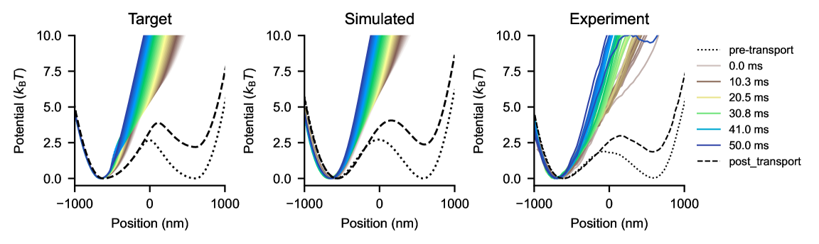
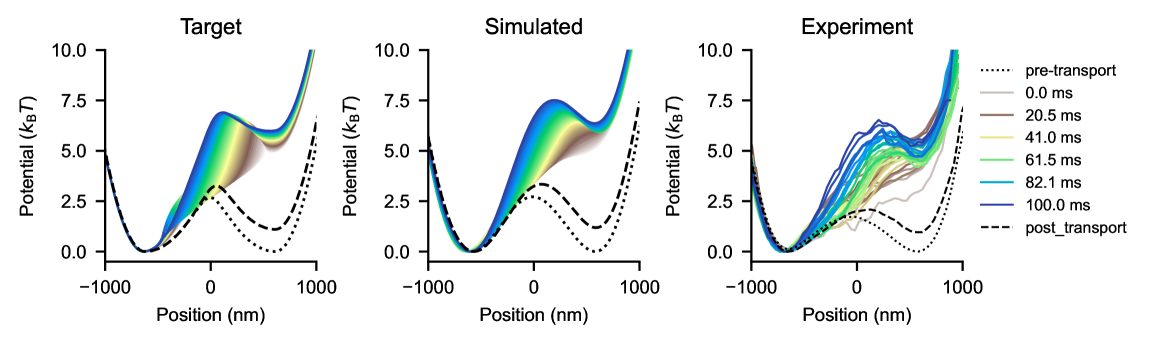
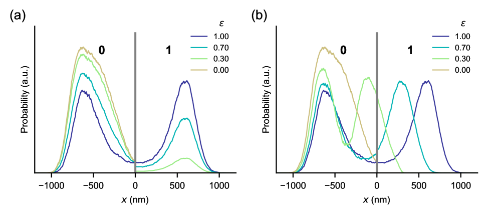
We now turn to the experiment on optimizing information erasure in finite time. Specifically, we consider a situation where one bit of information is encoded in a symmetric double-peak distribution, with logical state 0 assigned to and 1 assigned to (Fig. 3). The information erasure process transforms the double-peak distribution into a single-peak distribution corresponding to a fixed logical state. Without loss of generality, we focus on resetting to logical state 0, as the symmetric double-peak ensures the symmetry between 0 and 1.
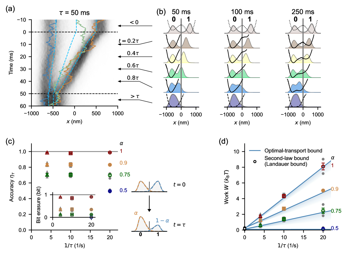
We experimentally implemented the optimal information erasure protocol that was obtained numerically (Fig. 3). The kymograph clarifies the distribution dynamics (Fig. 3a). The protocol translates the fraction of the distribution in the state 1 to the state 0. The fraction in 0 is slightly compressed leftward to save space for the incoming fraction from 1. As a result, we observed a linear variation of the tertiles and mean of the distribution (dashed curves in Fig. 3a). This is the characteristic of the optimal transport as shown in Fig. 1c (right). The optimal transport dynamics are similar for different when time is scaled by (Fig. 3b). This is also the characteristic of optimal transport and is realized by different potential dynamics depending on .
The accuracy of the information erasure is measured by the fraction of the state 0 at , denoted as . An almost perfect erasure with (mean standard deviation (s.d.)) was achieved even within finite time (Fig. 3c, ). Because the target final distribution has a tail extending beyond , perfect transport is not always expected. The corresponding bit erasure was bit (mean s.d., Fig. 3c, inset), which was quantified as . Here, is the Shanon information content defined in the natural logarithm, and . was (mean s.d.).
Work
We measured the work during the information erasure process (Fig. 3d, ). reached the finite-speed theoretical minimum given by within error bars, validating the realization of optimal finite-speed information erasure. is given by Eq. (1). The free energy difference corresponds to the Landauer bound, which can be reached in the quasi-static limit (). consists of the free energy change due to the bit erasure, Landauer1961, Berut2012, and the rearrangement of the particle distribution inside the 0 and 1 states Sagawa2014.
The values of evaluated solely from the distributions coincided with those from the recovered potential (Fig. 2g), again validating the effectiveness of the distribution-based evaluation of with this non-harmonic setup.
Energy-speed-accuracy trade-off
It is generally expected that more accurate control requires more work, and faster control reduces accuracy, implying the trade-off between energy cost , speed , and accuracy . To control the accuracy, we left a fraction of the distribution at so that the final distributions have double peaks; the height ratios of the two peaks are to (, see the right panel of Fig. 3c and SI Section S2.5). The distributions are designed so that they are approximately local equilibrium distributions in each well of a double-well potential. The accuracy increases with . However, does not solely determine , since the peaks have tails extending beyond as mentioned. We observed that the work become smaller with smaller as well as smaller (Fig. 3d), which implies the trade-off between energy cost, speed, and also accuracy. That is, a faster and more accurate process requires more work.
Figure 4 shows our experimental data in a way to clarify that they achieve the bound of the energy-speed-accurary trade-off. The values of for different collapsed into a single curve, which corresponds to the finite-time minimum predicted by the optimal transport theory (solid line, Eq. (1)). The fact that has a finite value independent of indicates that does not reach zero even in the quasi-static limit . The ordinary second law only claims the positivity of (dotted line). Since depends on , the results demonstrate the trade-off between , , and .

Discussion
In this study, we experimentally demonstrated thermodynamically optimal transport by implementing protocols that minimize dissipated work . We built a custom optical tweezer system capable of generating arbitrary potential profiles to optimize the distribution dynamics of Brownian microparticles in a thermal environment. We first demonstrated a simple transport problem of translating and compressing a Gaussian distribution, revealing the geometric structure of transport (Fig. 2). We then experimentally applied the optimal transport protocol to information erasure, achieving the finite-time Landauer bound, equivalent to Eq. (2) (Fig. 3). Our experiment achieved the trade-off bound between energy cost, speed, and accuracy (Fig. 4).
An approach that appears similar but is fundamentally distinct from optimal transport is optimal control Schmiedl2007, Blaber2023, Loos2024. While optimal transport directly optimizes the evolution of probability distributions, optimal control focuses on optimization through a certain set of potential parameters and thus does not necessarily produce the desired final distribution in finite time. This distinction becomes particularly relevant in the context of information erasure in finite time, where the erased information content is solely determined by the final compressed distribution but not by the specific profile of the final potential. In general, optimal control protocols differ from optimal transport protocols, as they are derived based on different optimization strategies (see also Extended Data Fig. 8 and SI Section S4).
We note that there is yet another approach to finite-time thermodynamic trade-offs, called thermodynamic uncertainty relations (TURs) Barato2015, Horowitz2019, which have been tested and used to estimate dissipation from experimental data Song2021, Marsland2019. However, the bounds provided by TURs are often unachievable through experiments. In contrast, the framework based on optimal transport theory provides an achievable bound (Eq. (1)) along with its optimal protocol, as experimentally demonstrated in this study.
Meanwhile, modern computers generate vast amounts of dissipation Ball2012, Markov2014. In the long term, their energetic efficiency will be fundamentally constrained by thermodynamic laws, such as the Landauer bound Landauer1961, Parrondo2015, Pigolotti-Peliti and its finite-time refinement (Eq. (2)). Our experiment highlights the crucial role of optimizing temporal dynamics in approaching such fundamental bounds. Given that CMOS technology underpins modern computing and operates far from the quasi-static limit, a fundamental challenge is whether its architecture can achieve such thermodynamic bounds Freitas2021, Wolpert2024. While our study serves as a proof-of-concept, it is expected to provide guiding principles for the design of more energy-efficient computing devices.
Acknowledgements
We thank Takayuki Ariga and Kenji Nishizawa for their technical assistance. This work was supported by JST ERATO Grant Numbers JPMJER2204 and JPMJER2302, and JSPS KAKENHI Grant Numbers 22H01141, 23H01136, 23H00467, and 24H00834.
Author Contributions
SO, YN, SI, TS, and ST designed the research and wrote the paper. SO performed experiments. SO, YN, and ST developed the experimental systems, contributed analytic tools, and analyzed data.
References
- 1 Monge, G. Mémoire sur la théorie des déblais et des remblais (De l’Imprimerie Royale, 1781).
- 2 Villani, C. Optimal transport: old and new (Springer, 2009).
- 3 Arjovsky, M., Chintala, S. & Bottou, L. Wasserstein generative adversarial networks. In Precup, D. & Teh, Y. W. (eds.) Proceedings of the 34th International Conference on Machine Learning (ICML 2017), vol. 70, 214–223 (PMLR, 2017).
- 4 Lipman, Y., Chen, R. T. Q., Ben-Hamu, H., Nickel, M. & Le, M. Flow matching for generative modeling. In The Eleventh International Conference on Learning Representations (2023).
- 5 Schiebinger, G. et al. Optimal-transport analysis of single-cell gene expression identifies developmental trajectories in reprogramming. \JournalTitleCell 176, 928–943.e22, DOI: 10.1016/j.cell.2019.01.006 (2019).
- 6 Aurell, E., Gawȩdzki, K., Mejía-Monasterio, C., Mohayaee, R. & Muratore-Ginanneschi, P. Refined second law of thermodynamics for fast random processes. \JournalTitleJ. Stat. Phys. 147, 487–505, DOI: 10.1007/s10955-012-0478-x (2012).
- 7 Nakazato, M. & Ito, S. Geometrical aspects of entropy production in stochastic thermodynamics based on Wasserstein distance. \JournalTitlePhys. Rev. Res. 3, 043093, DOI: 10.1103/physrevresearch.3.043093 (2021).
- 8 Proesmans, K., Ehrich, J. & Bechhoefer, J. Finite-time Landauer principle. \JournalTitlePhys. Rev. Lett. 125, 100602, DOI: 10.1103/physrevlett.125.100602 (2020).
- 9 Proesmans, K., Ehrich, J. & Bechhoefer, J. Optimal finite-time bit erasure under full control. \JournalTitlePhys. Rev. E 102, 032105, DOI: 10.1103/physreve.102.032105 (2020).
- 10 Landauer, R. Irreversibility and heat generation in the computing process. \JournalTitleIBM J. Res. Dev. 5, 183–191, DOI: 10.1147/rd.53.0183 (1961).
- 11 Parrondo, J. M. R., Horowitz, J. M. & Sagawa, T. Thermodynamics of information. \JournalTitleNature Phys. 11, 131–139, DOI: 10.1038/nphys3230 (2015).
- 12 Benamou, J.-D. & Brenier, Y. A computational fluid mechanics solution to the Monge–Kantorovich mass transfer problem. \JournalTitleNum. Math. 84, 375–393, DOI: 10.1007/s002110050002 (2000).
- 13 Aurell, E., Mejía-Monasterio, C. & Muratore-Ginanneschi, P. Optimal protocols and optimal transport in stochastic thermodynamics. \JournalTitlePhysical Review Letters 106, 250601, DOI: 10.1103/physrevlett.106.250601 (2011).
- 14 Chen, Y., Georgiou, T. T. & Tannenbaum, A. Stochastic control and nonequilibrium thermodynamics: Fundamental limits. \JournalTitleIEEE Transactions on Automatic Control 65, 2979–2991, DOI: 10.1109/TAC.2019.2939625 (2019).
- 15 Ito, S. Geometric thermodynamics for the Fokker–Planck equation: stochastic thermodynamic links between information geometry and optimal transport. \JournalTitleInformation Geometry 7, 441–483, DOI: 10.1007/s41884-023-00102-3 (2024).
- 16 Seifert, U. Stochastic thermodynamics, fluctuation theorems and molecular machines. \JournalTitleRep. Prog. Phys. 75, 126001, DOI: 10.1088/0034-4885/75/12/126001 (2012).
- 17 Ciliberto, S. Experiments in stochastic thermodynamics: Short history and perspectives. \JournalTitlePhys. Rev. X 7, 021051, DOI: 10.1103/physrevx.7.021051 (2017).
- 18 Peliti, L. & Pigolotti, S. Stochastic Thermodynamics: An Introduction (Princeton University Press, 2021).
- 19 Shiraishi, N., Saito, K. & Tasaki, H. Universal trade-off relation between power and efficiency for heat engines. \JournalTitlePhys. Rev. Lett. 117, 190601, DOI: 10.1103/physrevlett.117.190601 (2016).
- 20 Sagawa, T. & Ueda, M. Minimal energy cost for thermodynamic information processing: Measurement and information erasure. \JournalTitlePhys. Rev. Lett. 102, 250602, DOI: 10.1103/physrevlett.102.250602 (2009).
- 21 Lutz, E. & Ciliberto, S. Information: From Maxwell’s demon to Landauer’s eraser. \JournalTitlePhys. Today 68, 30–35, DOI: 10.1063/pt.3.2912 (2015).
- 22 Bérut, A. et al. Experimental verification of Landauer’s principle linking information and thermodynamics. \JournalTitleNature 483, 187–189, DOI: 10.1038/nature10872 (2012).
- 23 Jun, Y., Gavrilov, M. & Bechhoefer, J. High-precision test of Landauer’s principle in a feedback trap. \JournalTitlePhys. Rev. Lett. 113, 190601, DOI: 10.1103/physrevlett.113.190601 (2014).
- 24 Gavrilov, M. & Bechhoefer, J. Erasure without work in an asymmetric double-well potential. \JournalTitlePhys. Rev. Lett. 117, 200601, DOI: 10.1103/physrevlett.117.200601 (2016).
- 25 Ribezzi-Crivellari, M. & Ritort, F. Large work extraction and the Landauer limit in a continuous Maxwell demon. \JournalTitleNature Phys. 15, 660–664, DOI: 10.1038/s41567-019-0481-0 (2019).
- 26 Dago, S., Pereda, J., Barros, N., Ciliberto, S. & Bellon, L. Information and thermodynamics: Fast and precise approach to Landauer’s bound in an underdamped micromechanical oscillator. \JournalTitlePhys. Rev. Lett. 126, 170601, DOI: 10.1103/physrevlett.126.170601 (2021).
- 27 Dago, S., Ciliberto, S. & Bellon, L. Adiabatic computing for optimal thermodynamic efficiency of information processing. \JournalTitleProc. Nat. Acad. Sci. 120, e2301742120, DOI: 10.1073/pnas.2301742120 (2023).
- 28 Toyabe, S., Sagawa, T., Ueda, M., Muneyuki, E. & Sano, M. Experimental demonstration of information-to-energy conversion and validation of the generalized Jarzynski equality. \JournalTitleNature Phys. 6, 988–992, DOI: 10.1038/nphys1821 (2010).
- 29 Koski, J. V., Maisi, V. F., Pekola, J. P. & Averin, D. V. Experimental realization of a Szilard engine with a single electron. \JournalTitleProc. Nat. Acad. Sci. 111, 13786–13789, DOI: 10.1073/pnas.1406966111 (2014).
- 30 Toyabe, S. et al. Nonequilibrium energetics of a single F1-ATPase molecule. \JournalTitlePhys. Rev. Lett. 104, 198103, DOI: 10.1103/physrevlett.104.198103 (2010).
- 31 Di Terlizzi, I. et al. Variance sum rule for entropy production. \JournalTitleScience 383, 971–976, DOI: 10.1126/science.adh1823 (2024).
- 32 Hopfield, J. J. Kinetic proofreading: A new mechanism for reducing errors in biosynthetic processes requiring high specificity. \JournalTitleProc. Nat. Acad. Sci. 71, 4135–4139, DOI: 10.1073/pnas.71.10.4135 (1974).
- 33 Andrieux, D. & Gaspard, P. Nonequilibrium generation of information in copolymerization processes. \JournalTitleProc. Nat. Acad. Sci. 105, 9516–9521, DOI: 10.1073/pnas.0802049105 (2008).
- 34 Lan, G., Sartori, P., Neumann, S., Sourjik, V. & Tu, Y. The energy–speed–accuracy trade-off in sensory adaptation. \JournalTitleNature Phys. 8, 422–428, DOI: 10.1038/nphys2276 (2012).
- 35 Barato, A. C. & Seifert, U. Thermodynamic uncertainty relation for biomolecular processes. \JournalTitlePhys. Rev. Lett. 114, DOI: 10.1103/physrevlett.114.158101 (2015).
- 36 Dechant, A. Minimum entropy production, detailed balance and Wasserstein distance for continuous-time markov processes. \JournalTitleJournal of Physics A: Mathematical and Theoretical 55, 094001, DOI: 10.1088/1751-8121/ac4ac0 (2022).
- 37 Yoshimura, K., Kolchinsky, A., Dechant, A. & Ito, S. Housekeeping and excess entropy production for general nonlinear dynamics. \JournalTitlePhysical Review Research 5, 013017, DOI: 10.1103/PhysRevResearch.5.013017 (2023).
- 38 Vu, T. V. & Saito, K. Thermodynamic unification of optimal transport: Thermodynamic uncertainty relation, minimum dissipation, and thermodynamic speed limits. \JournalTitlePhys. Rev. X 13, 011013, DOI: 10.1103/physrevx.13.011013 (2023).
- 39 Klinger, J. & Rotskoff, G. M. Universal energy-speed-accuracy trade-offs in driven nonequilibrium systems. \JournalTitlePhys. Rev. E 111, DOI: 10.1103/physreve.111.014114 (2025).
- 40 Sagawa, T. Thermodynamic and logical reversibilities revisited. \JournalTitleJournal of Statistical Mechanics: Theory and Experiment 2014, P03025, DOI: 10.1088/1742-5468/2014/03/p03025 (2014).
- 41 Schmiedl, T. & Seifert, U. Optimal finite-time processes in stochastic thermodynamics. \JournalTitlePhys. Rev. Lett. 98, 108301, DOI: 10.1103/physrevlett.98.108301 (2007).
- 42 Blaber, S. & Sivak, D. A. Optimal control in stochastic thermodynamics. \JournalTitleJ. Phys. Comm. 7, 033001, DOI: 10.1088/2399-6528/acbf04 (2023).
- 43 Loos, S. A., Monter, S., Ginot, F. & Bechinger, C. Universal symmetry of optimal control at the microscale. \JournalTitlePhys. Rev. X 14, 021032, DOI: 10.1103/physrevx.14.021032 (2024).
- 44 Horowitz, J. M. & Gingrich, T. R. Thermodynamic uncertainty relations constrain non-equilibrium fluctuations. \JournalTitleNature Phys. 16, 15–20, DOI: 10.1038/s41567-019-0702-6 (2019).
- 45 Song, Y. & Hyeon, C. Thermodynamic uncertainty relation to assess biological processes. \JournalTitleJ. Chem. Phys. 154, 130901, DOI: 10.1063/5.0043671 (2021).
- 46 Marsland, R., Cui, W. & Horowitz, J. M. The thermodynamic uncertainty relation in biochemical oscillations. \JournalTitleJ. R. Soc. Interface 16, 20190098, DOI: 10.1098/rsif.2019.0098 (2019).
- 47 Ball, P. Computer engineering: Feeling the heat. \JournalTitleNature 492, 174–176, DOI: 10.1038/492174a (2012).
- 48 Markov, I. L. Limits on fundamental limits to computation. \JournalTitleNature 512, 147–154, DOI: 10.1038/nature13570 (2014).
- 49 Freitas, N., Delvenne, J.-C. & Esposito, M. Stochastic thermodynamics of nonlinear electronic circuits: A realistic framework for computing around kT. \JournalTitlePhys. Rev. X 11, DOI: 10.1103/physrevx.11.031064 (2021).
- 50 Wolpert, D. H. et al. Is stochastic thermodynamics the key to understanding the energy costs of computation? \JournalTitleProc. Nat. Acad. Sci. 121, DOI: 10.1073/pnas.2321112121 (2024).
Methods
Experimental setup
An infrared laser with a wavelength of (Spectra-Physics (MKS Instruments), MA) was focused through a 100 objective lens (NA1.40, Evident, Japan), specialized for a near-infrared laser, equipped to an inverted microscope (Evident) to create an optical trap (Extended Data Fig. 1). The laser power was adjusted by an attenuator (ThorLabs, NJ). The typical laser power at the sample was , which was measured by an optical power meter (ThorLabs).
We trapped a silica particle with a diameter of (Micromod, Germany) diluted by distilled water in an observation chamber with a height of . The trap position was approximately from the bottom glass surface. The chamber was made by sticking two pieces of coverslips (Matsunami, Japan) together with double-sided tape (Teraoka, Japan). The inlet and outlet of the channel were sealed with nail polish (DAISO, Japan) to prevent evaporation. The particle images were taken by a high-speed camera (Basler, Germany) at with an exposure time of under LED illumination (ThorLabs). The room temperature was . The experiments were controlled by LabVIEW software (NI, TX).
The laser focal point was scanned by an electro-optical deflector (Conoptics, CT) at to create a trapping potential. The translation speed was controlled so that the mean light intensity at each position is proportional to the designed value of the potential at each position. We deconvolved target potential profiles by Gaussian intensity profile that approximates the laser spot to obtain the scan pattern under constraints that the total power is fixed, the spatial scanning range is limited, and the mean time duration residing at each position is positive (Extended Data Fig. 9, see SI Section S1 for details).
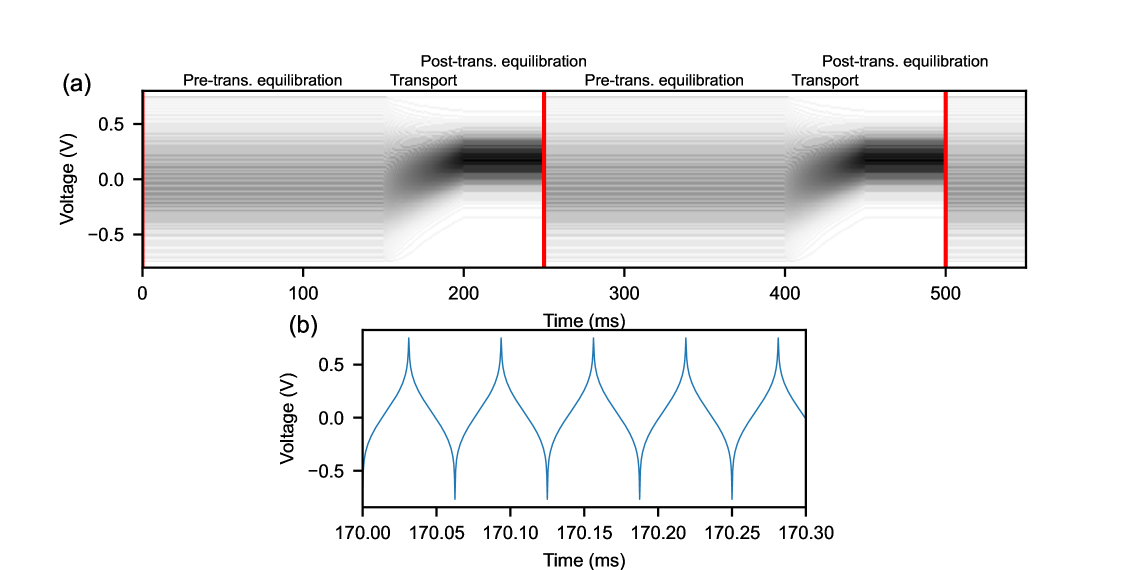
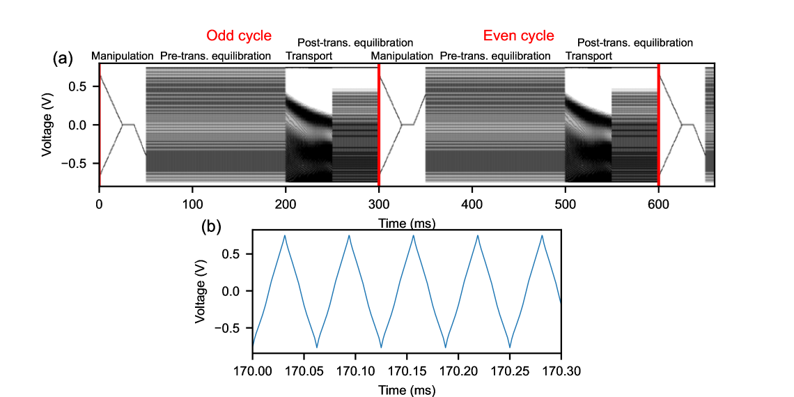
We repeated more than 3,000 repetitions for and 1,500 repetitions for in each run of the translation-compression protocols for a single particle and 5,000 repetitions in each run of the information-erasure protocols for a single particle. We conducted at least three runs with three different particles under each condition (actual numbers are specified in the figure captions). Each cycle of the repetitions consists of the following steps (Extended Data Figs. 2 and 3); initial manipulation, pre-transport equilibration, transport, and post-transport equilibration. The initial manipulation step is only used in the information erasure, which is intended for fast relaxation to the equilibrium of the initial state between 0 and 1.
The particle position was evaluated as the centroid of the particle image, , where is the pixel intensity at position . The threshold intensity is determined as the top 20% of the intensity distribution of the whole image. This fraction-based thresholding is expected to reduce the noise due to the temporal illumination variation. The sum was taken for the pixels in the largest cluster of the pixels with intensities larger than , which was further processed by erosion and dilation, to reduce the effect of noise. The precision evaluated as the s.d. of the centroid of a particle fixed on a glass surface was . This value is a composite value including other effects such as the oscillation of the camera, microscope body, and microscope stage.
Wasserstein distance and transport protocols
Think of transporting a one-dimensional distribution to . The transport map is expressed as such that . For given two one-dimensional distributions and , 2-Wasserstein distance is defined as
| (M1) |
subject to the Jacobian equation Villani2009. Here, denotes an Euclidean distance and is in one-dimensional systems. We used a Python library “POT: Python Optimal Transport” flamary2021pot for calculating the Wasserstein distance.
For an overdamped Langevin dynamics, the minimum transport cost is given by Eq. (1). The optimal transport that achieves this minimum is numerically obtained Benamou2000. In one-dimensional Euclidean space, the optimal transport is a linear transport without changing the positional order, such as leftmost to leftmost and center to center Villani2009 (Fig. 1c, right). The potential dynamics that realize this optimal transport are obtained by numerically solving the Fokker-Planck equation. See SI Section S2 for details, including the naive, gearshift, and intermediate protocols.
Evaluation of potential and work
The potential profile was recovered based on a drift velocity. By discretizing the Langevin equation , we obtain . Here, is the potential force, and is the white Gaussian noise with zero mean and unit variance. is a Wiener process. We obtain by splitting into spatial bins and calculating the average of in each bin, since the mean of is zero. was estimated as described below. Then, is recovered by integrating and then smoothed by a window averaging.
This method is applicable to trajectories that are not settled in equilibrium. We applied the method to the trajectories during transport, where the potential profile varies in time. For each video frame, we use multiple consecutive frames around that frame of all the repetitions in each run for better statistics to obtain the potential profile. We used 21 frames for and and 41 frames for . Slower dynamics with longer allow us to use more frames. Extended Data Figure 10 shows examples of the recovered potentials, which are quantitatively similar to the target potentials. The potential dynamics realized by the optical tweezers are constrained by the diffraction limit. The fact that the minimum dissipated work can still be obtained suggests that the rough transport design determines the dissipated work, and the specific details do not significantly affect it. This tolerance implies the effectiveness of the optimal transport theory in broad practical systems.
The dissipated work is calculated using Seifert2012, Pigolotti-Peliti
| (M2) | ||||
We calculated these values based on experimental trajectories as follows. Let and be the particle position and potential in the -th frame, respectively. The transport step corresponds to . and correspond to the last frame of the pre-transport step and the first frame of the post-transport step, respectively. was calculated as
| (M3) |
and are the potentials before and after the transport process, respectively. denotes the average between different repetitions. We obtained by calculating , , and . Here, specifies the spatial bin, and is the probability of being in the -th bin at -th frame. For the evaluation of , multiple frames (11 frames) around a target frame were used for better statistics.
Evaluation of the dissipated work from distribution dynamics
Consider dividing into short transport segments with time duration ( (Fig. 2f, inset). The dissipated work during -th segment, denoted as , is bound as
| (M4) |
By taking the summation over , we obtain . In the limit of , we expect that converges to since if we consider the one-dimensional Euclidean space where the nonconservative force does not exist Nakazato2021. Hence,
| (M5) |
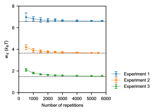
Equation (M5) enables us to evaluate only from the distribution dynamics without knowing the potential profiles or individual trajectories. Figure 2f, g demonstrates the validity of the method. Extended Data Figure 11 shows the dependence of evaluated from the distributions on the number of repetitions. The value of converges from above to a specific value. More than 3,000 repetitions are necessary for sufficient convergence in the present setup in the information erasure. We measured more than 5,000 repetitions, which is sufficient for the convergence.
Evaluation of friction coefficient
The friction coefficient of each particle was measured before the transport experiments. The power spectrum of the particle position obeys a Lorentzian spectrum in a harmonic potential (Extended Data Fig. 5):
| (M6) |
where is a frequency, is a corner frequency, and is the trap stiffness. is obtained by least-square fitting of with the fitting parameters and . The multiplication by biases the fitting weight to the frequency region around , which is intended to improve the fitting accuracy. The value of was (means.d.). This value is similar to that estimated by Stokes law, , where at (average room temperature) is the viscosity of water, and is the particle radius. Since the precise value of is also not known, the estimation by the Stokes law was used only as a reference.
Extended Data Figures


References
- 1 Villani, C. Optimal transport: old and new (Springer, 2009).
- 2 Flamary, R. et al. POT: Python Optimal Transport. \JournalTitleJ. Mach. Learn. Res. 22, 1–8 (2021).
- 3 Benamou, J.-D. & Brenier, Y. A computational fluid mechanics solution to the Monge–Kantorovich mass transfer problem. \JournalTitleNum. Math. 84, 375–393, DOI: 10.1007/s002110050002 (2000).
- 4 Seifert, U. Stochastic thermodynamics, fluctuation theorems and molecular machines. \JournalTitleRep. Prog. Phys. 75, 126001, DOI: 10.1088/0034-4885/75/12/126001 (2012).
- 5 Peliti, L. & Pigolotti, S. Stochastic Thermodynamics: An Introduction (Princeton University Press, 2021).
- 6 Nakazato, M. & Ito, S. Geometrical aspects of entropy production in stochastic thermodynamics based on Wasserstein distance. \JournalTitlePhys. Rev. Res. 3, 043093, DOI: 10.1103/physrevresearch.3.043093 (2021).
- 7 Schmiedl, T. & Seifert, U. Optimal finite-time processes in stochastic thermodynamics. \JournalTitlePhys. Rev. Lett. 98, 108301, DOI: 10.1103/physrevlett.98.108301 (2007).
Supplementary information for “Experimentally achieving minimal dissipation via thermodynamically optimal transport”
Shingo Oikawa, Yohei Nakayama, Sosuke Ito, Takahiro Sagawa, and Shoichi Toyabe
S1 Generation of laser scan pattern
The laser focal point was scanned by an electro-optical deflector at to create a trapping potential. The translation speed was adjusted so that the mean light intensity at each position is proportional to the target potential at each position. We deconvolved target potential profiles by Gaussian intensity profile that approximates the laser spot to obtain the scan pattern under constraints that the total power is fixed, the spatial scanning range is limited, and the mean time duration residing at each position is positive.
Let the intensity profile of a single laser spot be , which could be approximated by a Gaussian profile. The particle feels a potential proportional to at each location . Think that we scan the laser spot at a rate faster than the relaxation time of the particle, which is typically the ratio of the trapping spring constant and the friction coefficient of the particle (estimated to be in the order of in the present setup). Then, the particle feels only the mean light intensity at each position given by
| (S1) |
for a fixed scanning protocol. Here, is the laser position, and is the residential time fraction at . We modulate only the scan speed at each position and do not temporally modulate . Therefore, the total light intensity is constant. The particle feels a potential at each position proportional to , . is a proportional coefficient. Since is a constant independent of the scanning protocol, is also a constant. We obtain a similar expression to Eq. (S1),
| (S2) |
is the potential profile of a single laser spot.
is inferred by experiments as follows. We generate a Gaussian potential with a known value of the width . should has the form of with an unknown parameter , which will be determined by experiments. Since the particle is strongly trapped, we approximate as a harmonic potential with the effective spring constant . We measure from the width of the equilibrium distribution using . Finally, we obtain as .
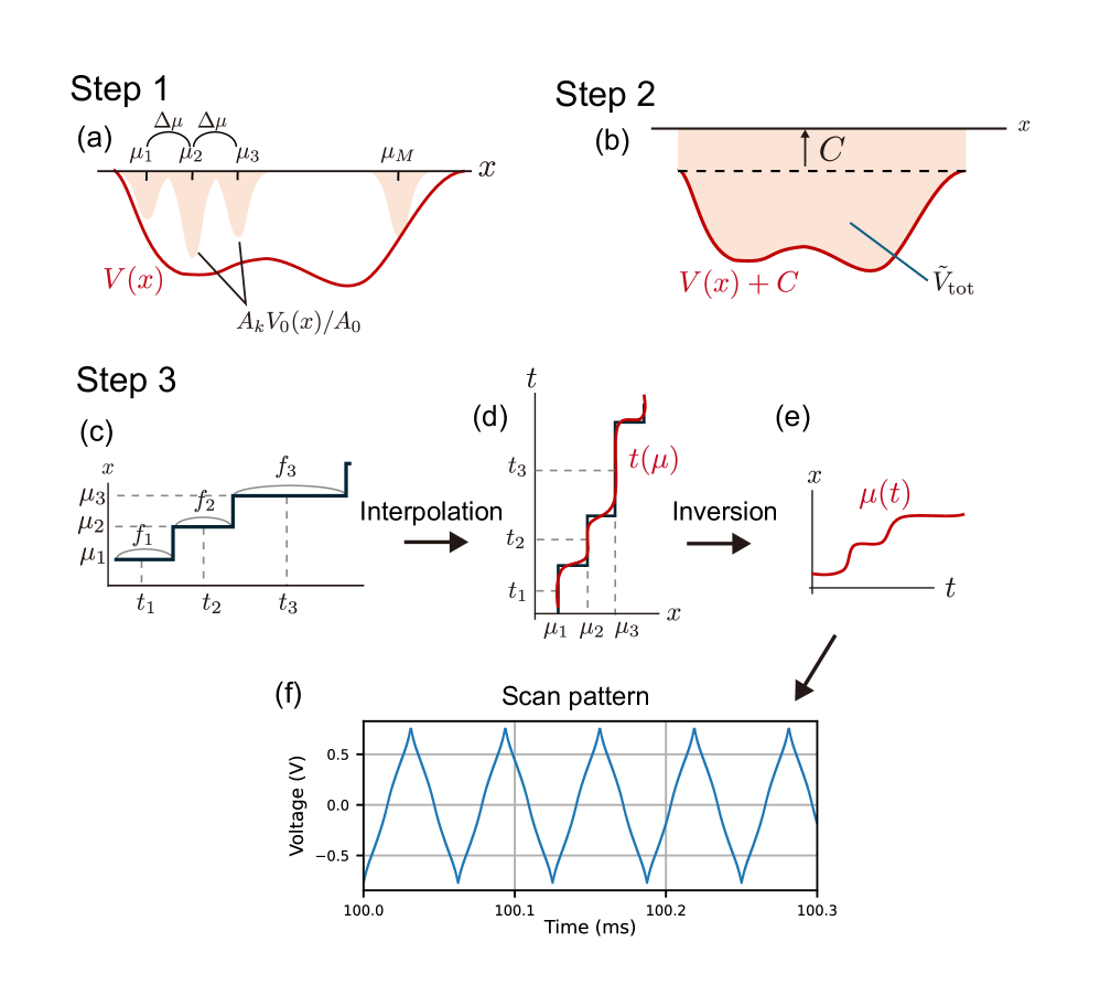
The actual workflow of the deconvolution and the generation of the scan pattern proceeds in the following three steps (Extended Data Fig. 9).
- Step 1.
-
The target potential is approximated by the superposition of elementary potentials located in the scan range between and (Extended Data Fig. 9a).
(S3) We used in the experiments. We assume that the laser spots are located at separated by , and each potential has a Gaussian profile . is the spot size of the laser. To evaluate , we generated a potential by scanning the laser at a high frequency between two locations in a distance of . The particle feels a double-well potential for and a single-well potential for . We measured to be as the threshold distance of by controlling and measuring the position distribution of the trapped particle.
We determine by minimizing a cost function defined as
(S4) The second term on the right-hand side is introduced so that neighboring peaks do not have large amplitude differences, which may cause distortions in the scan patterns in the experiments. and are constants and adjusted depending on the target potential profile. We used and . We find that minimize under the constraint of by trust region reflective algorithm of SciPy library 2020SciPy-NMeth.
- Step 2.
-
The total of the potential
(S5) should be a constant, , which is determined by an experiment, as explained. To satisfy this constraint, we introduce an offset such that
(S6) and modify the cost function as
(S7) Here, is the total of potential within . We iterate the update of and minimum finding of multiple times (21 times) to find the optimal values of under the constraint of (Extended Data Fig. 9b).
- Step 3.
-
We determine the laser scan pattern based on normalized peak intensities , which correspond to the residential time fraction of the laser spot at during the scan cycle (Extended Data Fig. 9c). The center of the duration is for , , and = 1. Accordingly, the spot locations are extended by adding and for the interpolation in the next step. is interpolated to obtain a continuous function (Extended Data Fig. 9d). The inversed function (Extended Data Fig. 9e) and are alternatively repeated to generate the scan pattern (Extended Data Fig. 9f).
The scan pattern was controlled by a computer equipped with LabVIEW and a multifunction card (NI, TX). The voltage update rate for EOD was . A diagonal direction of the two-dimensional EOD control was used to obtain the maximum travel distance.
To calibrate the laser power variation with position, we measured the spring constants of a harmonic potential generated by laser spots at fixed positions by fitting the distributions with Gaussians. The spring constants are measured 10 times each at 21 different locations for at each location. The dependence of the spring constant on the position was fitted by an eighth-order polynomial function.
S2 Optimal transport
S2.1 Computation of optimal transport
We used the optimal transport map to calculate the distribution dynamics under the optimal transport protocol . The optimal transport protocol in the one-dimensional Euclidean space translates each segment in the initial distribution to the final distribution linearly without changing the positional order of the segmentsVillani2009 (Fig. 1c, right). The optimal transport map describes where a segment at in is translated. The optimal transport map is related with as . The preservation of the positional order of the segments means
| (S8) |
where and are the cumulative distribution function at and , respectively. Since the translation is linear, a segment at in is translated to the position in . That is, the optimal cumulative distribution function satisfies
| (S9) |
Therefore, we first obtain by numerically solving Eq. (S8) and then calculate by numerically differentiating obtained from Eq. (S9).
The details of the calculation are as follows. To obtain , we find pairs of positions satisfying
| (S10) |
by the bisection method. Here, are chosen as
| (S11) |
where , , , , and . Since follows from Eq. (S8) and Eq. (S10), equal to . Therefore, is evalutaed as . We obtain at by numerically differentiating as
| (S12) |
and interpolate it as necessary.
S2.2 Computation of potential dynamics
Once distribution dynamics is obtained, we can calculate the potential dynamics that realizes by solving a Fokker-Planck equation,
| (S13) |
with boundary conditions at . Here,
| (S14) |
is the probability flux. We solve Eq. (S13) by splitting it into
| (S15) | ||||
| (S16) |
Eq. (S16) is obtained from Eq. (S14). We first obtain by integrating Eq. (S15), and then calculate by integrating Eq. (S16). For Gaussian dynamics, as in translation and compression protocols, we can derive simplified equations (Eq. (S19)).
To numerically integrate Eqs. (S15) and (S16), we consider a sufficiently wide interval and impose boundary conditions at and . We use at and to calculate and , where and are integers, , , , and . is obtained by summing up the discretized version of the left hand side of Eq. (S15) multiplied by , , where is a half-integer. To reduce the effect of numerical error, we calculate and by summing up from and , respectively. And then, we adopt for , for , and for as , where we choose
| (S17) |
Finally, we discretize the left hand side of Eq. (S16) as
| (S18) |
and obtain by summing up it.
S2.3 Translation and compression protocols
For Gaussian dynamics, the mean and width of the distribution obey
| (S19) |
where and are the position and the stiffness of a harmonic potential, respectively. Equation (S19) are deduced from the Fokker-Planck equation (Eq. (S13)), and leads to
| (S20) |
These relations provide and for given and .
The optimal transport corresponds to a linear translation of and between the initial and final distributions:
| (S21) |
The gearshift transport is a combination of two optimal transports with different translation speeds and time duration:
| (S22) | |||||
| (S23) |
and are the fractions of the distance and duration before the gearshift, respectively. We obtain and for the optimal and gearshift transports by using Eq. (S20).
The naive protocol linearly varies the position and stiffness of the potential as
| (S24) |
In the experiment, we generated Gaussian-profile potentials with a width of approximately . This width is sufficiently large so that the particle effectively feels a harmonic potential (Extended Data Fig. 10).
S2.4 Transports with intermediate optimality
The intermediate transports between the optimal and naive transports are obtained by simple interpolation:
| (S25) |
Here, is the interpolation parameter. and 1 correspond to the optimal and naive protocols, respectively. Given that the naive and optimal transports have the same initial and final distributions, , , , , the intermediate transport also has the same initial and final distributions.
Then, we can show that the dissipated work of this intermediate transport depends quadratically on as
| (S26) |
Equation (S26) is obtained as follows. In Gaussian processes, the dissipated work for () is given by
| (S27) |
where the square of the speed in distribution space is defined as
| (S28) |
To consider the dissipated work for (), we calculate as
| (S29) |
Since is independent of ,
| (S30) |
Therefore,
| (S31) |
From the same calculation for , we calculate as
| (S32) |
and thus we obtain Eq. (S26) by using the above equations and Eq. (S28) for (), () and ().
S2.5 Information erasure
The initial and final distributions, and , are designed by combining Gaussians with different widths:
| (S33) |
where
| (S34) |
We used the peak position , and the widths and . We used for the initial distribution. We varied of the final distribution to control the accuracy (, and 1).
S3 Energy-speed-accuracy trade-off
S3.1 Energy-speed-accuracy trade-off in terms of Wasserstein distance
In this paper, the accuracy of information erasure is quantified by , which is the fraction of 0 at (Figs. 3c and 4). In Ref.Klinger2025, the transport error is defined based on the Wasserstein distance. We apply this framework to the present experimental setup of the information erasure.
We define transport error by
| (S35) |
according to Ref.Klinger2025. Here, is a target distribution. We chose for and for , which corresponds to a perfect information erasure.
We can derive hierarchical trade-off relations between energy cost, speed, and accuracyKlinger2025. Let be the distribution with the same as and on the geodesic between and (Extended Data Fig. 7a). That is, satisfies . On the one hand, a triangle inequality and lead to . On the other hand, . Using these relations, hierarchical trade-off relations are derived:
| (S36) | ||||
| (S37) | ||||
| (S38) |
The first inequality (Eq. (S36)) corresponds to a bound of for given and (solid line in Extended Data Fig. 7b), which is achieved in the experiments (symbols). The equality is satisfied by the optimal transport, which is also indicated as solid lines in Fig. 3d and 4.
On the other hand, we can find other distributions that achieve smaller with the same . Equation (S37) gives the minimum of for given (dashed line in Extended Data Fig. 7b). Since is a constant for given and , the second inequality indicates the trade-off where smaller and require larger even if we change the choice of . While this bound is achieved when lies on the geodesic between and , such a distribution has a rather complicated profile and would not be practical for information processing (gray distribution series in Extended Data Fig. 7a, see also Extended Data Fig. 12b). In fact, if we finalize the transport protocol by a double-well potential, it costs additional dissipation for the relaxation to local equilibrium in each well Proesmans2020, Proesmans_2020-2. As noted, the present transport targets approximately local-equilibrium distributions in each well of a double-well potential (illustrated as green distribution series in Extended Data Fig. 7a).
S3.2 Relation between the transport error and accuracy
The above results demonstrate that, while is also a measure to quantify the accuracy of the transport, the Wasserstein distance provides a unified perspective on the trade-off by quantifying both the error and energy cost. We derive that is related to as under the assumption that is written as with a small parameter , and holds for .
We evaluate the optimal transport map to the leading order in . satisfies
| (S39) |
where and are the cumulative distribution functions given as and , respectively. For , is evaluated as
| (S40) |
Combining Eqs. (S39) and (S40) with , we obtain , or equivalently . Here, since for . Because is nonzero for and independent of , holds for . On the other hand, for , is evaluated as
| (S41) |
where . From Eq. (S39), we obtain for . Thus, and hold for .
From the above results, we obtain
| (S42) |
where we used for . As a result, is written as
| (S43) |
where
| (S44) |
is a coefficient independent of . Here, we used , which is obtained from for and . Therefore, is proportional to up to the order .
S4 Comparision between optimal transport and optimal control
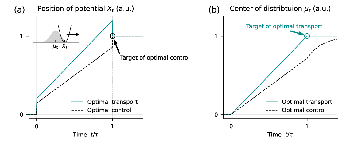
A similar but fundamentally distinct approach to minimization of dissipative work is the concept of optimal control, which seeks the optimal protocol for given initial and final control parameters instead of probability distributions.
A quantitative difference between optimal transport and optimal control is illustrated in Extended Data Fig. 8 for a simple translation protocol without compression, which translates a harmonic potential with a fixed spring constant. In such a situation, the distribution is always Gaussian with a constant width. Let be the position of a harmonic potential, and be the mean particle position.
The task of the optimal transport is to reach a given final distribution of the particle position at , which is a Gaussian with the center at , with the minimum dissipation. The optimal dynamics of has a forward jump at and a backward jump at (Extended Data Fig. 8a, blue curve). This results in a linear translation of , which reaches the given final position at (Extended Data Fig. 8b, blue curve).
On the other hand, the task of optimal control is to change a set of control parameters of the potentials to the final target values at with the minimum dissipation. In this situation, also has initial and final jumps, but both are in the forward direction, different from the optimal transport (Extended Data Fig. 8a, black dashed curve). This protocol translates the distribution linearly but does not reach the equilibrium distribution of the final target potential within finite time (Extended Data Fig. 8b, black dashed curve). The distribution relaxes to the equilibrium one in a sufficiently long time after . Thus, optimal control does not necessarily produce the desired final distribution in finite time.
Therefore, optimal transport and optimal control are based on fundamentally different strategies for different purposes. Optimal transport is more relevant for processes like information erasure, where one wants to produce the given final state 0 in finite time.
References
- 1 Virtanen, P. et al. SciPy 1.0: Fundamental Algorithms for Scientific Computing in Python. \JournalTitleNature Methods 17, 261–272, DOI: 10.1038/s41592-019-0686-2 (2020).
- 2 Villani, C. Optimal transport: old and new (Springer, 2009).
- 3 Klinger, J. & Rotskoff, G. M. Universal energy-speed-accuracy trade-offs in driven nonequilibrium systems. \JournalTitlePhys. Rev. E 111, DOI: 10.1103/physreve.111.014114 (2025).
- 4 Proesmans, K., Ehrich, J. & Bechhoefer, J. Finite-time Landauer principle. \JournalTitlePhys. Rev. Lett. 125, 100602, DOI: 10.1103/physrevlett.125.100602 (2020).
- 5 Proesmans, K., Ehrich, J. & Bechhoefer, J. Optimal finite-time bit erasure under full control. \JournalTitlePhys. Rev. E 102, 032105, DOI: 10.1103/physreve.102.032105 (2020).