∎
11email: yassine.nabou@helsinki.fi
This work has been supported by the Academy of Finland grant 345486.
Nonmonotone higher-order Taylor approximation methods for composite problems
Abstract
We study composite optimization problems in which the smooth part of the objective function is -times continuously differentiable, where is an integer. Higher-order methods are known to be effective for solving such problems, as they speed up convergence rates. These methods often require, or implicitly ensure, a monotonic decrease in the objective function across iterations. Maintaining this monotonicity typically requires that the -th derivative of the smooth part of the objective function is globally Lipschitz or that the generated iterates remain bounded. In this paper, we propose nonmonotone higher-order Taylor approximation (NHOTA) method for composite problems. Our method achieves the same nice global and rate of convergence properties as traditional higher-order methods while eliminating the need for global Lipschitz continuity assumptions, strict descent condition, or explicit boundedness of the iterates. Specifically, for nonconvex composite problems, we derive global convergence rate to a stationary point of order , where is the iteration counter. Moreover, when the objective function satisfies the Kurdyka–Łojasiewicz (KL) property, we obtain improved rates that depend on the KL parameter. Furthermore, for convex composite problems, our method achieves sublinear convergence rate of order in function values. Finally, preliminary numerical experiments on nonconvex phase retrieval problems highlight the promising performance of the proposed approach.
Keywords:
Composite problems, (Non)convex minimization, Higher-order methods, convergence rates.1 Introduction and motivation
In this paper, we consider the following composite optimization problem:
| (1) |
where is a -times continuously differentiable function, and is a proper, lower semicontinuous, and convex function. Here, is a finite-dimensional real vector space. Despite its simple form, this problem occur frequently in many applications including machine learning meier2008group , compressed sensing tibshirani1996regression , matrix factorization lee1999learning ; lin2007projected , (sparse) inverse covariance selection hsieh2011sparse ; oztoprak2012newton , blind deconvolution ayers1988iterative ; bertero1998novel . Further applications can be found in deep learning deleu2021structured , data clustering ravikumar2011high and dictionary learning mairal2009online .
First-Order Methods among the most popular methods for solving problems of the form (1). For example, proximal point (Prox) methods has been extensively studied and are widely recognized as one of the most effective approaches for solving optimization problems of the form (1), where the objective function consists of both a smooth and a non-smooth component. Prox method operates by iteratively refining the solution through a sequence of subproblems, each of which involves the proximal operator associated with the non-smooth part of the objective function. For a given current point , and in the context of solving problems (1), Prox method finds the next iterate by solving
where is the step size that controls the update magnitude. This implies that the new iterate is obtained by applying a quadratic approximation to the smooth function , while the nonsmooth function remains unmodified and is incorporated directly into the subproblem. It is well known and straightforward to verify that this procedure can be equivalently rewritten as
with
For a comprehensive analysis of this method, readers can refer to the seminal works by Nesterov nesterov2013gradient and Parikh & Boyd parikh2014proximal . Despite its widespread applicability and strong theoretical foundations, the proximal gradient method, like other first-order methods, their convergence speed is known to be slow. This limitation arises because first-order methods rely solely on gradient information, which may not fully capture the curvature of the objective function.
Second-order methods such as Newton-type methods are particularly appealing because they achieve superlinear or even polynomial convergence rates while efficiently escaping saddle points agarwal2017finding . The proximal Newton method extends classical Newton’s method to the composite setting lee2014proximal . In this approach, the smooth function is approximated by its second-order Taylor expansion, while the nonsmooth function remains unchanged and is incorporated directly into the subproblem. This allows the method to effectively leverage curvature information from while maintaining the structure of , leading to improved convergence behavior. However, classical Newton’s method lacks global convergence guarantees, as its performance heavily depends on the initialization and the local behavior of the Hessian. In particular, when the Hessian is ill-conditioned or singular, Newton’s updates can be unstable, leading to divergence or poor progress toward a solution. One approach to mitigate these issues is the regularized Newton method, which improves stability by adding a regularization term to the Hessian to ensure well-posed updates and better global behavior mishchenko2023regularized ; doikov2024gradient . Another approach, cubic regularization, addresses these instability issues by introducing a cubic term to control the step size adaptively nesterov2006cubic . Adaptive second-order methods with cubic regularization and inexact steps were proposed in cartis2011adaptive ; cartis2011adaptiveII . Moreover, these approaches achieves global convergence rates that are faster than those of first-order methods.
Higher-order methods extend the principles of first- and second-order methods by utilizing derivatives of the objective function beyond just the first (gradient) and second (Hessian) orders. These methods incorporate higher-order derivatives, such as third-order tensors or even higher, to build sophisticated higher-order Taylor models. The unpublished preprint baes2009estimate stands as the first paper deriving theoretical results of the higher-order schemes for convex problems. However the extensive complexity associated with minimizing nonconvex multivariate polynomials has posed significant challenges, rendering this initial effort unsuccessful. Despite these obstacles, a ray of hope emerged through the groundbreaking research of Nesterov in nesterov2021implementable . Specifically, Nesterov demonstrated that by appropriately regularizing the Taylor approximation, the auxiliary subproblem remains convex and can be solved efficiently, thereby offering a promising avenue for tackling convex unconstrained smooth problems. As researchers delve deeper into the intricacies of optimization methods, particularly within the nonconvex setting birgin2017worst ; cartis2019universal , a notable focus has been placed on analyzing the complexity of high-order approaches. These approaches aim to generate solutions with small gradient norms, a crucial aspect for navigating nonconvex optimization landscapes effectively. In addressing this challenge, it is essential for such methods to maintain a satisfactory adherence to first-order optimality conditions and ensure local reductions in the objective function. Convergence guarantees, particularly in terms of the norm of the gradient, have been established to be of order birgin2017worst ; cartis2019universal . High-order inexact tensor methods were considered in jiang2020unified ; agafonov2024inexact ; martinez2017high . Increasing the order of the oracle, denoted as , provides certain advantages. Despite the complexity involved, ongoing research efforts continues to explore the performance of high-order optimization methods in nonconvex settings, aiming for more robust and efficient techniques.
The aforementioned methods are generally monotone, meaning that they either require or implicitly ensure a monotonic decrease in the objective function. To maintain this monotonicity, it is typically necessary to assume that the smooth part of the objective function is globally Lipschitz continuous over the entire space or the prior assumption that the iterates generated by these methods remain bounded. Nonmonotone first-order methods have been developed, which relax these assumptions and allow for more flexible descent mechanisms. Unlike traditional monotone schemes which require or enforce a strict decrease in the objective function along the iterates, nonmonotone methods allow occasional increases in function value while still guaranteeing overall convergence (see, e.g., zhang2004nonmonotone ; kanzow2022convergence ; de2023proximal ; kanzow2024convergence ; qian2024convergence ). This flexibility can be particularly beneficial for composite optimization problems, where strict descent conditions might delay progress or slow convergence. For example, kanzow2024convergence considered a nonmonotone proximal gradient method for minimizing problem (1), assuming that is locally Lipschitz, and is bounded below by an affine function. Under these mild assumptions, kanzow2024convergence derives global convergence rates that essentially have the same rate of convergence properties as its monotone counterparts. While existing works on higher-order methods typically assume global Lipschitz continuity of the higher-order derivatives, and their convergence analysis relies on establishing a strict descent in the objective function, in this paper, we propose a nonmonotone higher-order method that does not depend on these conditions. Instead, our approach relaxes the standard smoothness assumptions and allows for a more flexible descent mechanism, enabling improved performance in settings where global Lipschitz properties do not hold or are difficult to verify.
Contributions. We propose NHOTA, a Nonmonotone Higher-Order Taylor Approximation methods for solving composite optimization problems (1). Our approach leverages higher-order Taylor approximations combined with nonmonotone techniques, allowing us to establish global convergence rates without requiring global Lipschitz continuity and/or boundedness of the iterates. Our contributions can be summarized as follows:
-
1.
We introduce NHOTA, a higher-order tensor method that incorporates nonmonotonicity technique to solve composite problems (1).
-
2.
We derive global convergence guarantees for NHOTA under mild assumptions for nonconvex composite problems. Specifically, we show that the iterates generated by NHOTA converge to a stationary points and the convergence rate is of order , where is the iteration counter. Additionally, when the objective function satisfies a Kurdyka-Łojasiewicz (KL) property, we derive linear/sublinear convergence rates in function values, depending on the parameter of the KL condition.
-
3.
For convex composite problems, we derive a global sublinear convergence rate in function values, and the convergence rate is of order .
-
4.
Our results are obtained without requiring global Lipschitz continuity assumptions, boundedness of the iterates, or the traditional monotonicity condition in the objective along the iterates, thereby broadening the applicability of NHOTA.
Contents. The remaining parts of this paper are organized as follows. In Section 2, we discuss the basic properties required for our analysis. In Section 3, we introduce our method, NHOTA. Section 4 presents global/local convergence guarantees for NHOTA for nonconvex composite problems, followed by the analysis of the convergence rate for convex composite problems in Section 5. In Section 6, we present numerical illustrations of NHOTA on nonconvex phase retrieval problems. Finally, Section 7 concludes the paper and suggests directions for future work.
2 Notations and preliminaries
We denote a finite-dimensional real vector space with and its dual space composed of linear functions on . For any linear function , the value of at point is denoted by . Using a self-adjoint positive-definite operator , we endow these spaces with conjugate Euclidean norms:
For a twice differentiable function on a convex and open domain , we denote by and its gradient and hessian evaluated at , respectively. Then, and for all , . Throughout the paper, we consider positive integers. In what follows, we often work with directional derivatives of function at along directions of order , , with . If all the directions are the same, we use the notation , for If is times differentiable, then is a symmetric -linear form, and its norm is defined as:
Further, the Taylor approximation of order of the function at is denoted with:
Let be a differentiable function on the open domain . Then, the derivative is locally Lipschitz continuous if for any compact set , there exist a constant such that the following relation holds:
| (2) |
It is known that if (2) holds, then the residual between the function and its Taylor approximation can be bounded nesterov2021implementable :
| (3) |
If , we also have the following inequalities valid for all :
| (4) | ||||
| (5) |
For the Hessian, the norm defined in (5) corresponds to the spectral norm of self-adjoint linear operator (maximal module of all eigenvalues computed w.r.t. ). For a convex function , we denote by its subdifferential at that is defined by . Denote . Let us also recall the definition of a function satisfying the Kurdyka-Lojasiewicz (KL) property (see bolte2007clarke for more details).
Definition 1
A proper lower semicontinuous function satisfies Kurdyka-Lojasiewicz (KL) property on the compact set on which takes a constant value if there exist such that one has:
| (6) |
where is concave differentiable function satisfying and .
This definition is satisfied by a large class of functions, for example, functions that are semialgebric (e.g., real polynomial functions), vector or matrix (semi)norms (e.g., with rational number), see bolte2007clarke for a comprehensive list. For example, if is semi-algebraic function, then we have , with and bolte2007lojasiewicz . Then, the KL property establishes the following local geometry of the nonconvex function around a compact set :
| (7) |
3 Nonmonotone higher-order Tensor method
In this section, we introduce our method along with the necessary assumptions for its analysis. To ensure clarity and simplicity in the presentation, we define the following notation, where represents a constant that will be used throughout the discussion
| (8) |
For problem (1), we consider the following assumptions
Assumption 1
We have the following assumptions on the problem (1)
-
1.
The function is bounded from below over its domain.
-
2.
The function is a proper, lower semicontinuous, and convex function that is bounded from below by an affine function.
-
3.
The function is -times differentiable, and is locally Lipschitz continuous.
Note that Assumption 1 is fundamental in analyzing nonmonotone schemes de2023proximal ; kanzow2022convergence ; kanzow2024convergence . Indeed, the first condition is introduced to ensure the well-posedness of the problem (1), while the local Lipschitz condition is equivalent to being Lipschitz continuous on any compact set. Moreover, this local Lipschitz property is a significantly weaker condition than the usual global Lipschitz assumption. For instance, the exponential function, the natural logarithm, and all polynomials of degree higher than are locally Lipschitz but not globally Lipschitz on their respective domains. In higher-order methods, it is usually shown that the objective function is strictly decreasing along the iterates, or a backtracking technique is employed to ensure this decrease. A key observation is that the next iterate, , is required to satisfy the following strict descent inequality:
for a given . This is generally guaranteed under some global Lipschitz continuity of the -th derivative of the smooth part of the objective, or by ensuring that the iterates remain bounded (e.g., birgin2017worst ; nabou2024efficiency ). Building on the works of kanzow2024convergence ; qian2024convergence ; zhang2004nonmonotone , our method is designed to enforce the following condition, which plays a crucial role in ensuring convergence
where the reference function depends on past iterates. This formulation leverages historical information to provide a more flexible and potentially more effective descent mechanism compared to traditional approaches. Following kanzow2024convergence ; zhang2004nonmonotone , is computed as a convex combination of the previous reference value and the new function value . Our method is defined in Algorithm 3.1.
| (9) |
It is well known that if is convex and , where is the Lipschitz constant of the -th derivative of , then the model defined in (8) is convex (see nesterov2021implementable ). However, in the absence of , there is no guarantee that the subproblem (8) remains convex for a given , and thus the model (8) is generally nonconvex. Therefore, each iteration of NHOTA involves the approximate minimization of the model , as defined in (8), satisfying conditions (9). It is important to note that this condition is relatively mild, as it only requires a decrease in the regularized -th order model and the identification of an approximate first-order stationary point birgin2017worst ; grapiglia2020tensor ; martinez2017high . No global optimization of this potentially nonconvex model is required.
4 Nonconvex convergence analysis
In this section, we derive the global convergence results for the proposed method, establishing the conditions under which the method converges to a stationary point. The analysis will be based on the assumptions introduced earlier and will highlight the key factors contributing to the global convergence of the algorithm.
Lemma 1
Proof
Let’s prove (1). Suppose that the inner loop in step 4 does not terminate after a finite number of steps in iteration . Recall that satisfies
Since as and given that is bounded below by an affine function, we obtain that as . Consequently, for any constant , there exists such that for all , we have . Using the local Lipschitz property, we then deduce the existence of satisfying for all
Thus, summing up the last two inequality we obtain
Further, there exist such that we have . This implies
| (11) |
Next, it remains to prove for all . Indeed, by recurrence, for , it follows immediately since . Assume that we have . Then, combining (11) with the update in Algorithm 3.1 (line 5) we get
| (12) |
Therefore, combining this inequality with the updates of , we get:
This proves our first claim. Further, combining (12) with the update of yields
Hence
This proves our second assertion. ∎
Remark 1
Lemma 1 demonstrates that the sequence is monotonically decreasing. Next, we will derive global convergence rate based on this descent, without requiring strict descent in the objective. Define the following level sets . Consequently, we have for all . Indeed, since is decreasing, we obtain
The following theorem derives global convergence of NHOTA under Assumption 1 and that the level sets is bounded, i.e., there exists such that .
Theorem 4.1
Proof
Since is bounded, then the sequence generated by NHOTA is bounded. Using Assumption 1 and (4), there exists such that
Then, we get for all
Further, combining this inequality with the descent (10), we obtain
| (14) |
Summing up this inequality, we get
where the last inequality follows from for all . Hence
This proves our assertion. ∎
Remark 2
Theorem 4.1 proves that the iterates generated by NHOTA converge to a stationary point and the convergence rate is of order , which is the standard convergence rate for higher-order algorithms for (unconstrained) nonconvex problems using higher-order derivatives birgin2017worst ; cartis2019universal ; nabou2024efficiency . In our convergence analysis, we emphasize that we do not rely on any global Lipschitz continuity assumptions or a strict descent condition in the objective function. As a result, our approach is more general and applicable to a broader class of problems, making it more flexible compared to traditional methods that require such conditions.
4.1 Improved convergence rates under KL
In this section, we derive convergence rates for the proposed method under the Kurdyka-Łojasiewicz (KL) property (1). To achieve this, we assume that the objective is a continuous function, meaning that is continuous. We establish improved convergence rates, proving linear or sublinear convergence in function values for the sequence generated by NHOTA. We denote the set of limit points of by .
The next lemma derives some properties for .
Lemma 2
Let the assumptions of Theorem 4.1 hold. Additionally, assume that is continuous. Then, we have , is compact and connected set, and is constant on , i.e., .
Proof
Let us prove that is constant. From the descent (10) we have that is monotonically decreasing, and since is assumed to be bounded from below and that , it converges. Let us say to , i.e., as . Further, we have , then
Since we have , then as . On the other hand, let be a limit point of the sequence . This means that there exists a subsequence such that . Since is continuous, we get and hence, we have . The closeness property of implies that , and thus . This proves that is a stationary point of and thus is nonempty. By observing that can be viewed as an intersection of compact sets, so it is also compact. The connectedness follows from bolte2014proximal . This completes the proof.
Next, we derive improved convergence rates in function values for the sequence generated by NHOTA.
Theorem 4.2
Proof
From the definition of , we have
where the first equality follows from the definition of , the first inequality follows from (7), the second inequality follows from (14), the third inequality follows from the. descent (10) Then, we get
where . Let us denote . Thus we obtain
rearranging the above inequality, it follows that
Subsequently, we derive the following recurrence
Using Lemma 6 in nabou2024efficiency with and that , our assertions follow. ∎
Remark 3
In this section, we have derived improved convergence rates in terms of function values for sequence generated by NHOTA, by leveraging higher-order information to solve problem (1). As mentioned in our previous remark, our convergence analysis does not rely on global Lipschitz continuity assumptions or a strict descent condition in the objective function, making our approach more general and applicable to a broader class of nonconvex optimization problems.
5 Convex convergence analysis
In this section, we assume that is a convex function, and we define as the global minimum of . Convexity ensures that any local minimum is also a global minimum, making the problem well-posed. We aim to establish global convergence rate for the iterates generated by NHOTA 3.1 in the context of convex composite optimization problems. Specifically, we demonstrate that the iterates converge to the global minimum and establish a sublinear convergence rate function values. Recall that and define the constants , . We now present the global convergence rate for convex composite problems.
Theorem 5.1
Let Assumption 1 be satisfied and additionally assume that is bounded. Let be convex function and be generated by NHOTA. Then, the sequence converges to . Moreover, if then have the following convergence rate
| (15) |
Otherwise, if we have
| (16) |
Proof
Note that since is decreasing and , then converges and thus . Further, from the update of (line 7 in NHOTA 3.1) and the convexity of , we get
| (17) |
for , the last inequality follows from the boundedness of diameter of . Then combining the last inequality with (4), we get
Denote . As a result, we obtain
implies
| (18) |
Furthermore, since and , then and thus we obtain the following recurrence
| (19) |
Given that is decreasing and bounded from below by , then . Let as consider the following two cases. If , then we get
Consequently, it follows
On the other hand, if then
Thus, for , the recursive inequality is as follows
Using lemma A.1 in nesterov2022inexact with , we get
This proves our claim. ∎
Remark 4
In Theorem 5.1, we establish convergence rate guarantees based on the quantity . Specifically, if , we obtain a linear convergence rate in function value. Conversely, if , we prove a sublinear convergence rate of order for convex composite optimization problems, which aligns with the typical convergence rates of higher-order methods for convex (unconstrained) problems nesterov2021implementable ; nabou2024efficiency . As mentioned in our previous remark, our convergence analysis does not rely on global Lipschitz continuity assumptions or a strict descent condition in the objective function, making our approach more general and applicable to a broader class of convex optimization problems of the form (1).
6 Numerical illustrations
In this section, we evaluate the performance of the proposed method for nonconvex phase retrieval problems candes2015phase with norm regularization. Our implementation was carried out on a MacBook M2 with 16GB of RAM, using the Julia programming language.
6.1 Nonconvex phase retrieval
In our experiments we apply NHOTA for to solve the following nonconvex phase retrieval problem with regularization:
| (20) |
where represents the observed measurements, and are the sensing vectors. This problem follows the structure of the composite problems (1) with and . Since the function is a polynomial of degree four, its Hessian is not globally Lipschitz continuous, which fits our setting as we do not require this property. The data is generated as follows: we set , , and , where the samples are generated element-wise, with denoting the true underlying object. The measurements are generated as
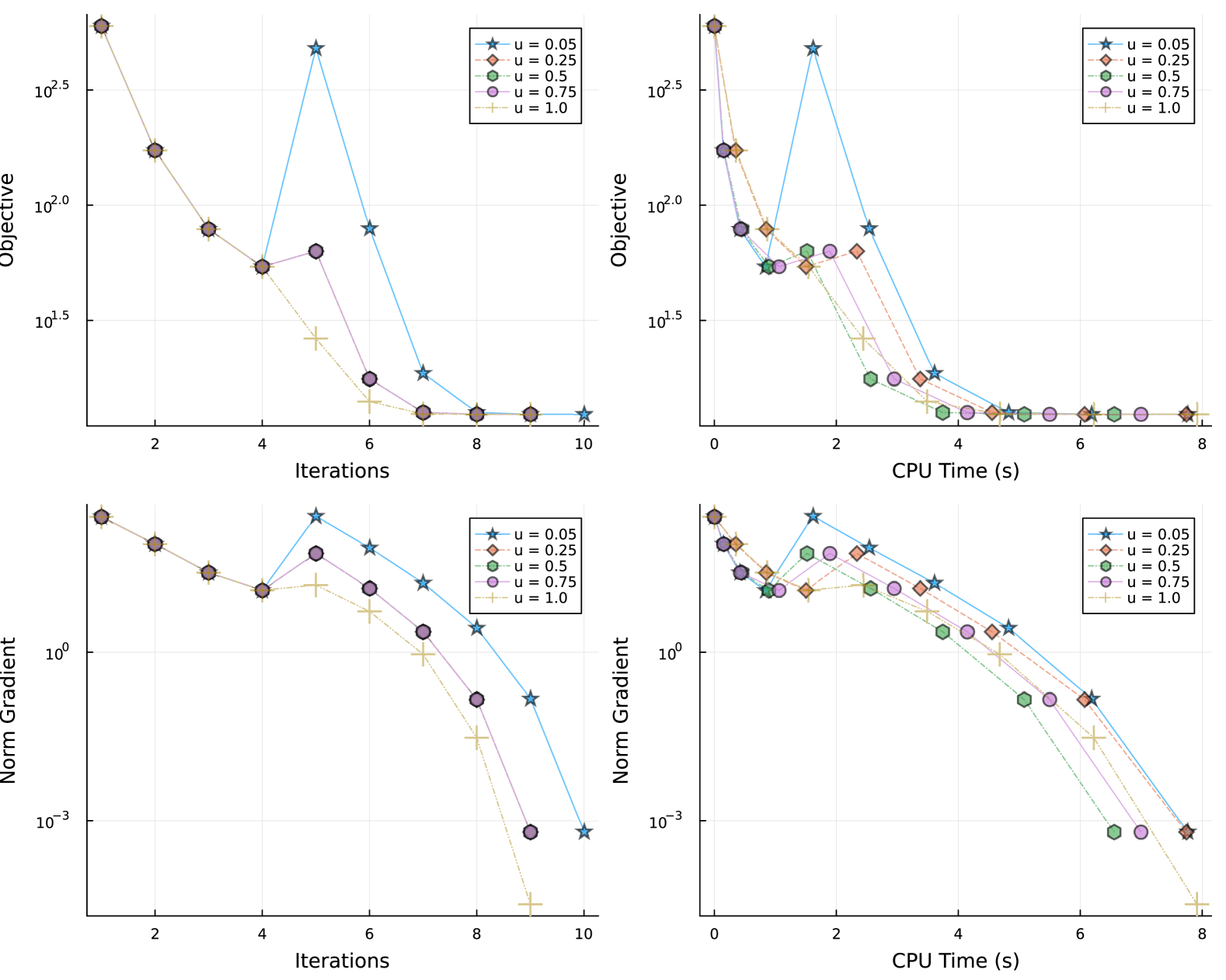
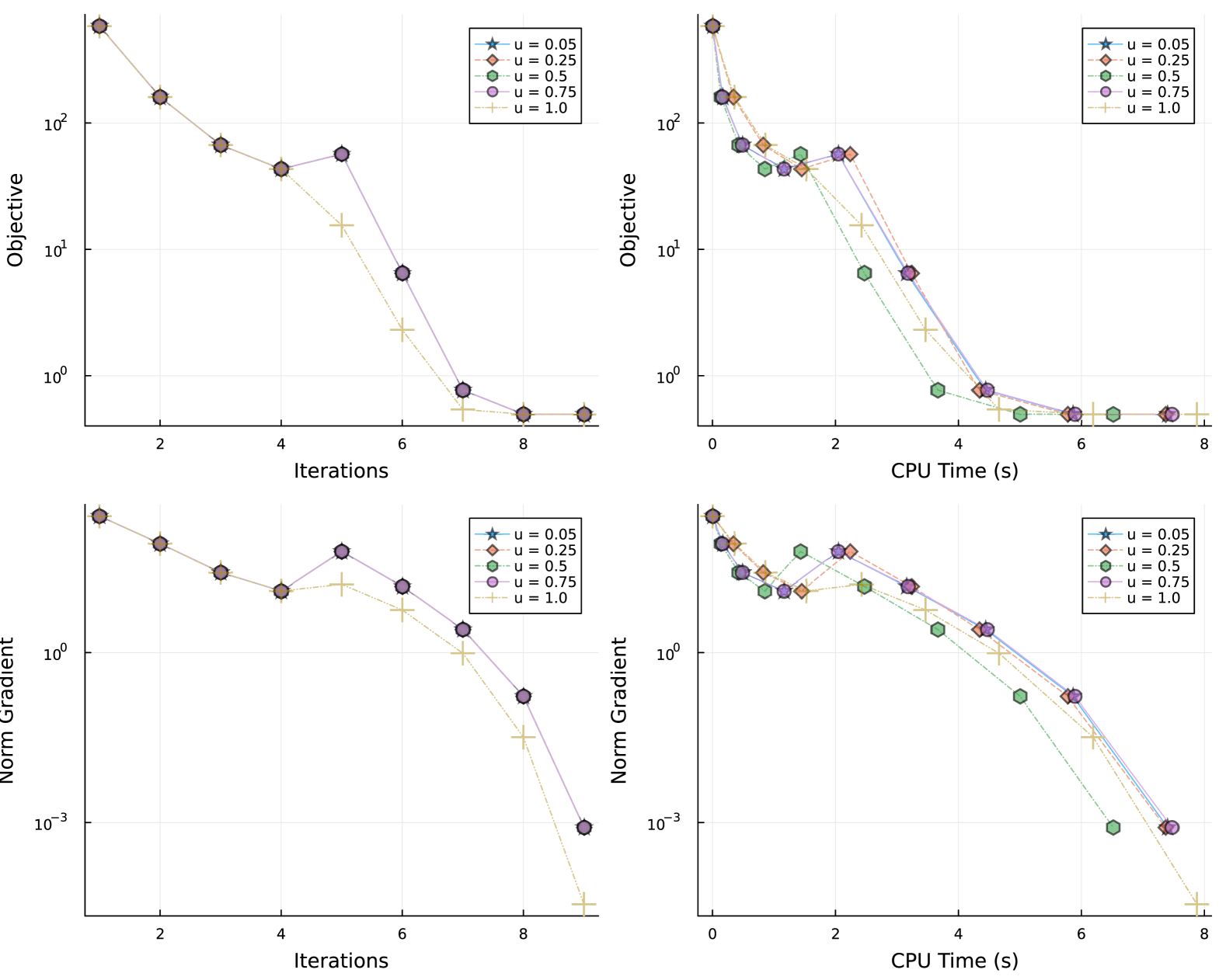
where represents random noise, and we set the regularization parameter to . The proposed method is evaluated for different fixed values of across iterations, for all , as specified in line 7 of Algorithm 3.1. All subproblems are solved using IPOPT wachter2006implementation . The results, shown in Figure 1, indicate that all choices of lead to convergence to a stationary point and a significant reduction in the objective function, depending on the noise level. Notably, when , the objective function decreases monotonically, whereas for , it does not necessarily follow a strictly decreasing trend. However, despite this lack of strict monotonicity, the final accuracy remains comparable to that of the monotone case, suggesting that allowing some flexibility in descent does not compromise solution quality. Regarding computational efficiency, it is difficult to determine an optimal choice for , but cases where tend to perform better in terms of CPU time. This is likely because the algorithm does not enforce strict monotonicity in these cases, potentially allowing for larger step sizes and reducing the number of backtracking steps, leading to lower overall computational cost. We run the proposed method for different fixed values of for all , as specified in line 7 of Algorithm 3.1. The stopping criterion used is either or (we omit the term for all due to and , as its contribution is negligible). All subproblems are solved using IPOPT wachter2006implementation , and the results are presented in Figure 1. Our first remark is that regardless of the chosen , all cases successfully converge to a stationary point and achieve a significant reduction in the objective function/norm of the gradient depending of the noise level. A key observation is that when , the objective function does not strictly decrease along the iterates, in contrast to the case when , where it exhibits monotonic descent. However, despite this lack of strict monotonicity, the non-monotone cases () produce a first-order solution similar to that of the monotone setting (). This suggests that allowing some flexibility in the descent process does not necessarily compromise solution quality. Finally, when analyzing performance with respect to computational time, it is difficult to determine a clear optimal choice for . Interestingly, some cases where tend to perform better than in terms of CPU efficiency. This can be attributed to the fact that when , the algorithm does not strictly enforce a monotonic decrease in the objective function. At the same time, it does not necessarily require more iterations than the monotone case, which may allow for larger step sizes in certain iterations. As a result, the backtracking procedure may take fewer steps in these cases, leading to a reduction in overall computation time. In conclusion, we believe that for certain applications, using smaller values of (i.e., ) could potentially achieve better accuracy than the fully monotone case (). However, we cannot provide a definitive answer at this stage. In future work, we plan to investigate this approach across different applications to gain a deeper understanding of its impact.
7 Conclusion
In this paper, we propose NHOTA, a Nonmonotone Higher-Order Taylor Approximation method for solving composite optimization problems. Our approach leverages higher-order tensor methods while avoiding traditional assumptions such as global Lipschitz continuity or strict descent conditions on the objective function. We derive global convergence guarantees for convex and nonxonvex composite problems, demonstrating that NHOTA achieves a convergence rate of order in the nonconvex setting, with improved rates under the Kurdyka-Łojasiewicz (KL) property, and achieves sublinear convergence rate of order in the convex case. These results highlight that NHOTA maintains the efficiency of classical higher-order methods while offering flexibility and broader applicability. Several directions remain open for future research. First, extending NHOTA to composition, smooth constrained, and nonlinear least squares optimization problems nabou2024efficiency ; nabou2024moving ; Yass2024 and analyzing its behavior would provide valuable insights. Furthermore, developing an accelerated variant of the proposed method for convex problems presents an interesting direction for future research nesterov2021implementable ; nesterov2022inexact ; grapiglia2020tensor . Another promising direction is the efficient implementation of NHOTA on modern hardware to accelerate large-scale optimization tasks, since the computational of solving the model remains a concern, particularly when using -th derivatives for , which may be impractical in many applications. Finally, extending our results for to the regularized Newton method mishchenko2023regularized ; doikov2024gradient is another interesting direction.
References
- (1) A. Agafonov, D. Kamzolov, P. Dvurechensky, A. Gasnikov, and M. Takáč, Inexact tensor methods and their application to stochastic convex optimization, Optimization Methods and Software 39 (2024), 42–83.
- (2) N. Agarwal, Z. Allen-Zhu, B. Bullins, E. Hazan, and T. Ma, Finding approximate local minima faster than gradient descent, in Proceedings of the 49th Annual ACM SIGACT Symposium on Theory of Computing, 2017, 1195–1199.
- (3) G. Ayers and J. C. Dainty, Iterative blind deconvolution method and its applications, Optics letters 13 (1988), 547–549.
- (4) M. Baes, Estimate sequence methods: extensions and approximations, Institute for Operations Research, ETH, Zürich, Switzerland 2 (2009).
- (5) M. Bertero, D. Bindi, P. Boccacci, M. Cattaneo, C. Eva, and V. Lanza, A novel blind-deconvolution method with an application to seismology, Inverse Problems 14 (1998), 815.
- (6) E. G. Birgin, J. Gardenghi, J. M. Martínez, S. A. Santos, and P. L. Toint, Worst-case evaluation complexity for unconstrained nonlinear optimization using high-order regularized models, Mathematical Programming 163 (2017), 359–368.
- (7) J. Bolte, A. Daniilidis, and A. Lewis, The Łojasiewicz inequality for nonsmooth subanalytic functions with applications to subgradient dynamical systems, SIAM Journal on Optimization 17 (2007), 1205–1223.
- (8) J. Bolte, A. Daniilidis, A. Lewis, and M. Shiota, Clarke subgradients of stratifiable functions, SIAM Journal on Optimization 18 (2007), 556–572.
- (9) J. Bolte, S. Sabach, and M. Teboulle, Proximal alternating linearized minimization for nonconvex and nonsmooth problems, Mathematical Programming 146 (2014), 459–494.
- (10) E. J. Candes, X. Li, and M. Soltanolkotabi, Phase retrieval via Wirtinger flow: Theory and algorithms, IEEE Transactions on Information Theory 61 (2015), 1985–2007.
- (11) C. Cartis, N. I. Gould, and P. L. Toint, Adaptive cubic regularisation methods for unconstrained optimization. Part I: motivation, convergence and numerical results, Mathematical Programming 127 (2011), 245–295.
- (12) C. Cartis, N. I. Gould, and P. L. Toint, Adaptive cubic regularisation methods for unconstrained optimization. Part II: worst-case function-and derivative-evaluation complexity, Mathematical programming 130 (2011), 295–319.
- (13) C. Cartis, N. I. Gould, and P. L. Toint, Universal regularization methods: varying the power, the smoothness and the accuracy, SIAM Journal on Optimization 29 (2019), 595–615.
- (14) A. De Marchi, Proximal gradient methods beyond monotony, Journal of Nonsmooth Analysis and Optimization 4 (2023).
- (15) T. Deleu and Y. Bengio, Structured sparsity inducing adaptive optimizers for deep learning, arXiv preprint arXiv:2102.03869 (2021).
- (16) N. Doikov and Y. Nesterov, Gradient regularization of Newton method with Bregman distances, Mathematical programming 204 (2024), 1–25.
- (17) G. N. Grapiglia and Y. Nesterov, Tensor methods for minimizing convex functions with Hölder continuous higher-order derivatives, SIAM Journal on Optimization 30 (2020), 2750–2779.
- (18) C. J. Hsieh, I. Dhillon, P. Ravikumar, and M. Sustik, Sparse inverse covariance matrix estimation using quadratic approximation, Advances in neural information processing systems 24 (2011).
- (19) B. Jiang, T. Lin, and S. Zhang, A unified adaptive tensor approximation scheme to accelerate composite convex optimization, SIAM Journal on Optimization 30 (2020), 2897–2926.
- (20) C. Kanzow and L. Lehmann, Convergence of Nonmonotone Proximal Gradient Methods under the Kurdyka-Lojasiewicz Property without a Global Lipschitz Assumption, arXiv preprint arXiv:2411.12376 (2024).
- (21) C. Kanzow and P. Mehlitz, Convergence properties of monotone and nonmonotone proximal gradient methods revisited, Journal of Optimization Theory and Applications 195 (2022), 624–646.
- (22) D. D. Lee and H. S. Seung, Learning the parts of objects by non-negative matrix factorization, nature 401 (1999), 788–791.
- (23) J. D. Lee, Y. Sun, and M. A. Saunders, Proximal Newton-type methods for minimizing composite functions, SIAM Journal on Optimization 24 (2014), 1420–1443.
- (24) C. J. Lin, Projected gradient methods for nonnegative matrix factorization, Neural computation 19 (2007), 2756–2779.
- (25) J. Mairal, F. Bach, J. Ponce, and G. Sapiro, Online dictionary learning for sparse coding, in Proceedings of the 26th annual international conference on machine learning, 2009, 689–696.
- (26) J. M. Martínez, On high-order model regularization for constrained optimization, SIAM Journal on Optimization 27 (2017), 2447–2458.
- (27) L. Meier, S. Van De Geer, and P. Bühlmann, The group lasso for logistic regression, Journal of the Royal Statistical Society Series B: Statistical Methodology 70 (2008), 53–71.
- (28) K. Mishchenko, Regularized Newton method with global convergence, SIAM Journal on Optimization 33 (2023), 1440–1462.
- (29) Y. Nabou and I. Necoara, Efficiency of higher-order algorithms for minimizing composite functions, Computational Optimization and Applications 87 (2024), 441–473.
- (30) Y. Nabou and I. Necoara, Moving higher-order Taylor approximations method for smooth constrained minimization problems, arXiv preprint arXiv:2402.15022 (2024).
- (31) Y. Nabou and I. Necoara, Regularized higher-order Taylor approximation methods for nonlinear least-squares (2024). Submitted for publication.
- (32) Y. Nesterov, Gradient methods for minimizing composite functions, Mathematical programming 140 (2013), 125–161.
- (33) Y. Nesterov, Implementable tensor methods in unconstrained convex optimization, Mathematical Programming 186 (2021), 157–183.
- (34) Y. Nesterov, Inexact basic tensor methods for some classes of convex optimization problems, Optimization Methods and Software 37 (2022), 878–906.
- (35) Y. Nesterov and B. T. Polyak, Cubic regularization of Newton method and its global performance, Mathematical programming 108 (2006), 177–205.
- (36) F. Oztoprak, J. Nocedal, S. Rennie, and P. A. Olsen, Newton-like methods for sparse inverse covariance estimation, Advances in neural information processing systems 25 (2012).
- (37) N. Parikh, S. Boyd, et al., Proximal algorithms, Foundations and trends® in Optimization 1 (2014), 127–239.
- (38) Y. Qian, T. Tao, S. Pan, and H. Qi, Convergence of ZH-type nonmonotone descent method for Kurdyka–Łojasiewicz optimization problems, arXiv preprint arXiv:2406.05740 (2024).
- (39) P. Ravikumar, M. J. Wainwright, G. Raskutti, and B. Yu, High-dimensional covariance estimation by minimizing l 1-penalized log-determinant divergence, Electronic Journal of Statistics 5 (2011).
- (40) R. Tibshirani, Regression shrinkage and selection via the lasso, Journal of the Royal Statistical Society Series B: Statistical Methodology 58 (1996), 267–288.
- (41) A. Wächter and L. T. Biegler, On the implementation of an interior-point filter line-search algorithm for large-scale nonlinear programming, Mathematical programming 106 (2006), 25–57.
- (42) H. Zhang and W. W. Hager, A nonmonotone line search technique and its application to unconstrained optimization, SIAM journal on Optimization 14 (2004), 1043–1056.