Algebraic approaches for the decomposition of reaction networks and the determination of existence and number of steady states

Abstract

Chemical reaction network theory provides powerful tools for rigorously understanding chemical reactions and the dynamical systems and differential equations that represent them. A frequent issue with mathematical analyses of these networks is the reliance on explicit parameter values which in many cases cannot be determined experimentally. This can make analyzing a dynamical system infeasible, particularly when the size of the system is large. One approach is to analyze subnetworks of the full network and use the results for a full analysis.

Our focus is on the equilibria of reaction networks. Gröbner basis computation is a useful approach for solving the polynomial equations which correspond to equilibria of a dynamical system. We identify a class of networks for which Gröbner basis computations of subnetworks can be used to reconstruct the more expensive Gröbner basis computation of the whole network. We compliment this result with tools to determine if a steady state can exist, and if so, how many.

Keywords: chemical reaction networks, steady states, Gröbner bases

1 Introduction

Chemical reaction network theory primarily consists of models of chemical or biochemical phenomena based on ordinary differential equations (ODEs). The kinetics associated with a network determine the rate at which the reactions occur, and once specified they determine the ODE system. Horn and Jackson [18] showed that a network endowed with mass-action kinetics always induces a polynomial ODE system. The coefficients for these polynomials are rate constants associated with the reactions. A goal of reaction network theory is to provide qualitative results applicable to reaction networks without fixing parameters, so that these results are applicable to networks with a range of parameters.

Chemical concentrations cannot always be measured or determined experimentally during the course of a reaction. Taking a measurement may alter the reaction. As a result, longitudinal data is not always available. In the absence of longitudinal data, parameter estimation must be based on data available at steady state.

When comparing reaction network models we will examine how well they each fit experimental data at steady states, by looking at the steady-state ideal induced by the reaction network.

Even at steady state, it may not be possible to measure the concentrations of certain chemical species. In this case, one approach is to remove those chemicals from the network model. The remaining system can then be parameterized from experimental data.

To compensate for the removal of these chemical species, their rate constants are incorporated into the reaction network model by replacing mass-action terms with rational expressions, such as Monod or Michaelis-Menten terms. The coefficients in the reaction-rate functions would then need to be estimated using measurements of chemical concentrations at different time points, assuming this data is available.

We will use an approach that first decomposes the network into subnetworks before completely removing a problematic species from a subnetwork [16]. This decomposition has a biological interpretation and context for the corresponding reaction network and subnetworks.

Beyond advantages with respect to data availability, the steady states of reaction networks are often the subject of an inquiry. In particular the existence of positive steady states, the number of steady states, and the stability of steady states are often of interest. Even for relatively simple or small polynomial ODE systems these questions can be difficult.

We also survey and apply some general algebraic methods for answering questions regarding the existence and number of positive steady states. The strength of these tools should be evident from the size and complexity of the particular reaction networks to which we apply them.

1.1 Preliminaries

In this section we will formally define a reaction network and its attendant parts. We denote the set of $n$-tuples of positive real numbers by $\mathbb{R}_{+}^{n}$, and for $x,y\in\mathbb{R}_{+}^{n}$ we write $x^{y}=(x_{1}^{y_{1}},x_{2}^{y_{2}},...,x_{n}^{y_{n}})$. We write $\mathcal{S}=\{X_{1},X_{2},\dotsc,X_{n}\}$, and identify $\mathbb{R}^{\mathcal{S}}:=\mathbb{R}^{n}$. Following the conventions used by Feinberg in [13], we denote a reaction network by $\mathcal{N}=\{\mathcal{S},\mathcal{C},\mathcal{R}\}$ where $\mathcal{S}$ is the set of species in the network; $\mathcal{C}$ is a set of vectors in $\overline{\mathbb{R}_{+}^{\mathcal{S}}}$, called the complexes in the network; $\mathcal{R}\subset\mathcal{C}\times\mathcal{C}$ is a subset called the reactions of the network, where $(y,y)\not\in\mathcal{R}$ for all $y\in\mathcal{C}$, and we write $y\to y^{\prime}$ when $(y,y^{\prime})\in\mathcal{R}$.

For $y\to y^{\prime}\in\mathcal{R}$, the corresponding reaction vector is $y^{\prime}-y\in\overline{\mathbb{R}}^{\mathcal{S}}$. The stoichiometric subspace is $S\coloneqq\text{span}\{{y^{\prime}-y\in\mathbb{R}^{\mathcal{S}}:y\to y^{\prime}\in\mathcal{R}}\}$. A kinetics for a reaction network is an assignment of a continuously differentiable rate function $\mathcal{K}_{y\to y^{\prime}}:\overline{\mathbb{R}}_{+}^{\mathcal{S}}\to\overline{\mathbb{R}}_{+}$ such that $\mathcal{K}_{y\to y^{\prime}}(c)>0$ if and only if $\operatorname{supp}(y)\subset\operatorname{supp}(c)$. A reaction network $\mathcal{N}$ together with a kinetics $\mathcal{K}$ is called a kinetic system (KS). A kinetics $\mathcal{K}$ for a reaction network is mass-action if, for each $y\to y^{\prime}\in\mathcal{R}$, there exists $k_{y\to y^{\prime}}\in\mathbb{R}_{+}$ such that

$$\mathcal{K}_{y\to y^{\prime}}(c)=k_{y\to y^{\prime}}{\displaystyle\prod_{s\in\mathcal{S}}c_{s}^{y_{s}}},$$ (1)

where $y_{s}$ is the stoichiometric coefficient for species $s$ in $y$, $k_{y\to y^{\prime}}$ is the rate constant of reaction $y\to y^{\prime}$, and $c_{s}$ is the molar concentration of species $s$. All the reaction networks will be assumed to have mass-action kinetics unless explicitly stated otherwise. The species formation rate function is

$$f(c)\coloneqq\sum_{\mathcal{R}}k_{y\to y^{\prime}}c^{y}(y^{\prime}-y).$$ (2)

for $c\in\overline{\mathbb{R}}_{+}^{\mathcal{S}}$ and its entries are called the system polynomials of $\mathcal{N}$. The steady state ideal is $I_{N}\coloneqq\langle f_{1}(x),\dotsc,f_{n}(x)\rangle\subseteq\mathbb{Q}[\kappa;x]$. The stoichiometric matrix associated with $\mathcal{N}$ and denoted by $N$ is the $|\mathcal{S}|\times|\mathcal{R}|$ matrix with entries in $\mathbb{Z}$ where each column corresponds to the reaction vector $y\to y^{\prime}$. We call $\operatorname{rank}(N)$ the rank of the network.

A conservation matrix $W\in\mathbb{R}^{(n-s)\times n}$ is any rank $n-s$ matrix that satisfies $WN=0$, that is $W$ is a left kernel of $N$. The corank of $N$ is the rank of $W$. For each $c\in\mathbb{R}^{n-s}$ we have an associated stoichiometric compatibility class given by $\mathcal{P}_{c}\coloneqq\{x\in\mathbb{R}^{n}_{\geq 0}:Wx=c\}.$ We note that $\mathcal{P}_{c}=\emptyset$ if $c\notin W(\mathbb{R}^{n}_{\geq 0})$. The positive stoichiometric compatibility class is simply $\mathcal{P}_{c}^{+}\coloneqq\mathcal{P}_{c}\cap\mathbb{R}^{n}_{>0}.$

When considering trajectories, we will want to think of the paths taken by single points in the space $\mathbb{R}_{+}^{\mathcal{S}}$. We refer to such a points as a composition, denoted by $c$ or $c^{\prime}$. A composition $c\in\mathbb{R}^{n}$ can reach a composition $c^{\prime}\in\mathbb{R}^{n}$ only if $c-c^{\prime}$ lies in the same stoichiometric compatibility class. For a mass-action kinetic system, a steady state, fixed point or equilibrium of the system is a point $c\in\mathbb{R}^{\mathcal{S}}$ such that $f(c)=0.$ The set of equilibria is $V=\{x\in\mathbb{R}^{n}_{\geq 0}|f(x)=0\}.$ A positive equilibrium $c^{*}$ is an equilibrium with the added restriction that $c^{*}\in\mathbb{R}_{+}^{\mathcal{S}}$ The set of positive equilibria is $V_{+}=\{x\in\mathbb{R}^{n}_{+}|f(x)=0\}.$ Retaining the notations above, for $\xi\in\mathbb{R}$, $x\in\mathbb{R}^{n}_{\geq 0}$, and $\omega$ a row of $W$, any equation of the form $\omega\cdot x=\xi$ is a conservation relation. Then $\mathcal{N}$ is conservative if $S\cap\mathbb{R}^{\mathcal{S}}_{+}\neq\emptyset.$

We now shift our focus to the algebraic definitions and constructions; see Section $9.6$ of [8]. The variable ordering we choose when our species are labeled $X_{1},...X_{n}$ will be the natural ordering of the subscript, that is $X_{1}>X_{2}>...>X_{n}$. Let $k$ be a field and $k[X]=k[x_{1},...,x_{n}]$ be the polynomial ring with base field $k$. For a monomial $m=X_{1}^{\alpha_{1}}...X_{n}^{\alpha_{n}}$ with $\alpha_{i}\in\mathbb{Z}_{\geq 0}$, the multidegree of $m$ is $\partial(m)\coloneqq(\alpha_{1},\alpha_{2},...,\alpha_{n})$. A monomial ordering is a well ordering $\geq$ on the set of monomials that satisfies $mm_{1}\geq mm_{2}$, whenever $m_{1}\geq m_{2}$ for monomials $m,m_{1},m_{2}$.

There are many different kinds of monomial orderings; we recall two of the most important. Let $m_{1}=X_{1}^{\alpha_{1}}...X_{n}^{\alpha_{n}}$, $m_{2}=X_{1}^{\beta_{1}}...X_{n}^{\beta_{n}}$ for $\alpha_{i},\beta_{i}\in\mathbb{Z}_{\geq 0}$. The lexicographic monomial ordering is the monomial ordering determined by ordering $m_{1},m_{2}$ by the left-most nonzero component of their difference, e.g., $m_{1}\geq_{lex}m_{2}$ if the left-most nonzero entry of $\partial(m_{1})-\partial(m_{2})$ is greater than zero. The graded reverse lexicographic monomial ordering is the monomial ordering determined by ordering $m_{1},m_{2}$ where $m_{1}\geq_{lex}m_{2}$ if

$$\sum_{i=1}^{n}\alpha_{i}>\sum_{i=1}^{n}\beta_{i}.$$

In the case of equality, the right-most nonzero entry of $\partial(m_{2})-\partial(m_{1})$ determines the order. We set $m_{1}\geq_{lex}m_{2}$ if the right-most nonzero entry of $\partial(m_{2})-\partial(m_{1})$ is greater than zero.

Given a monomial ordering $\geq$, the leading term of $f(X)$ is its monomial term of maximal order with respect to $\geq$ and is denoted $LT(f)$. If $I$ is an ideal in $k[x_{1},...,x_{n}]$, the leading term ideal denoted by $LT(I)$ is the ideal generated by the leading terms of all the elements in the ideal, $LT(I)=(LT(f)|f\in I).$ A Gröbner basis $G$ of an ideal $I$ is a set of generators for the ideal, i.e., $\langle LT(G)\rangle=\langle LT(I)\rangle.$

A vital question is if a reaction network has the capacity to admit exactly one steady state (monotstationary) or more than one steady state (multistationary), based solely on its structure. Numerical approaches, including parameter estimation, are computationally costly in most cases of moderately sized or complicated reaction networks. A theoretical approach that answers this more qualitative question would be very useful. Methods exist that can answer this question, without the need for numerical simulation or experimental data, but are inconclusive if certain conditions on the reaction network are not met. This is more frequent when the pathway for a phenomenon is not well understood, so that researchers are unsure about the fidelity of a proposed reaction network model for the phenomenon. Another issue with some of the methods is the reliance on the network to admit only specific kinetics for the model. Since we are focused on mass-action kinetics, we will mention when any of the conclusions are applicable to kinetics other than mass-action.

Discussed in length in [13], the deficiency-based theory is very strong. It has criteria that is easily checked, after which we can draw a conclusion depending on if the reaction network is weakly reversible or not. To discuss the theorem, we first need to introduce a few more definitions.

Following [13], we denote connectivity of $y$ and $y^{\prime}$ by $y\xleftrightarrow{}y^{\prime}$, if either $y\to y^{\prime}\in\mathcal{R}$ or $y^{\prime}\to y\in\mathcal{R}$. A linkage class $\mathcal{L}_{1}$ for reaction network $\mathcal{N}$ is a subset of $\mathcal{C}$ such that for any $y,y^{\prime}\in\mathcal{L}_{1}$ then $y\xleftrightarrow{}y^{\prime}$. We denote the number of linkage classes by $\ell$ and the linkage classes themselves by $\mathcal{L}_{i}$.

When looking at the dynamics of a reaction network we care about the directions the reactions take place. Let $\mathcal{N}=\{\mathcal{S},\mathcal{C},\mathcal{R}\}$ be a reaction network. We say that a complex $y\in\mathcal{C}$ ultimately reacts to a complex $y^{\prime}\in\mathcal{C}$ (written as $y\Rightarrow y^{\prime}$) if any of the following are true:

1. $y=y^{\prime}$,

2. $y\xrightarrow{}y^{\prime}$,

3. there exists a sequence of complexes $y_{1},...,y_{k}$ such that

   $$y\xrightarrow{}y_{1}\xrightarrow{}...\xrightarrow{}y_{k}\xrightarrow{}y^{\prime}.$$

If we also require that whenever $y\Rightarrow y^{\prime}$ we also have $y^{\prime}\Rightarrow y$, then this induces an equivalence relation on the set of complexes $\mathcal{C}$ and thus a partition of $\mathcal{C}$ into strong linkage classes. A strong linkage class for reaction network $\mathcal{N}$ is simply a subset of complexes all belonging to the same strong linkage class. A reaction network $\mathcal{N}$ is weakly reversible if every linkage class of a reaction network is a strong linkage class, i.e., for any $y\xleftrightarrow{}y^{\prime}$, we have $y\Rightarrow y^{\prime}$ and $y^{\prime}\Rightarrow y$. We call a strong linkage class $\tau\subseteq\mathcal{C}$ a terminal strong linkage class if for every complex $y\in\tau$ and any reaction $y\to y^{\prime}$, we have $y^{\prime}\in\tau$. We denote the number of terminal strong linkage classes by $t$.

The deficiency of a reaction network $\mathcal{N}=\{\mathcal{S},\mathcal{C},\mathcal{R}\}$, with $|\mathcal{C}|=m$, $s=\operatorname{rank}(\mathcal{N})$ and $\ell$ linkage classes, is denoted by $\delta$ and is defined as $\delta\coloneqq m-s-\ell$. The deficiency of a reaction network does not give us an idea of how big it is. It does, however, give us an idea of how connected the network is. That is, the lower the deficiency of a network, the fewer linear dependencies the network has. Deficiency-zero reaction networks are as linearly independent as the partition of linkage classes allows. Furthermore, any subnetwork of a deficiency-zero network will also have deficiency zero.

One of the oldest and most important results in Deficiency theory, which first appeared in the manuscripts by Feinberg [11], Horn [17], and Horn & Jackson [18], is the Deficiency Zero theorem,

Theorem 1 (Feinberg, Horn, Jackson).

Let $\mathcal{N}=\{\mathcal{S},\mathcal{C},\mathcal{R}\}$ be a reaction network such that $\delta=0$.

1. If $\mathcal{N}$ is not weakly reversible then for any kinetics $\mathcal{K}$ the set of positive equilibria is empty, that is $V\cap\mathcal{P}_{c}^{+}=\emptyset$.

2. If $\mathcal{N}$ is weakly reversible and has mass-action kinetics then each positive stoichiometric class admits exactly one positive equilibrium,

   $$|V\cap\mathcal{P}_{c}^{+}|=1.$$

   Furthermore this equilibrium is asymptotically stable.

If $s_{i}$ is the rank of linkage class $i$, then it can be shown that $s\leq\sum_{i=1}^{\ell}s_{i}$. The deficiency of linkage class $i$ can then be written as $\delta_{i}=m_{i}-1-s_{i}$, where $m_{i}$ is the size of linkage class $i$ (the number of complexes belonging to it). It can then be shown that

$$\sum_{i=1}^{\ell}\delta_{i}=\sum_{i=1}^{\ell}(n_{i}-1-s_{i})=n-\ell-\sum_{i=1}^{\ell}s_{i}\leq\delta.$$ (3)

We get $\delta=\sum_{i=1}^{\ell}\delta_{i}$ when $s=\sum_{i=1}^{\ell}s_{i}$, which occurs when the linkage classes are as independent from one another as possible, for example when combining two disjoint reaction networks (two networks are disjoint if $\mathcal{S}_{1}\cap\mathcal{S}_{2}=\emptyset$).

Further reading on advances on higher deficiency theorems can be found in Ellison [10] and [19].

2 Theoretical results on joining and decomposing chemical reaction networks

In systems biology it is very often that one finds distinct models trying to describe the same phenomenon. This is particularly true when the process is difficult to study. This could arise when incomplete data on the phenomenon is collected. One way to distinguish between models in this scenario is by comparing the Gröbner bases of the ideals that are generated by the system polynomials associated with each system. The biggest issue with this approach is that computational complexity grows very quickly as the number of species increases, even for moderately sized networks (between 10 and 20 species). Increased connectivity also increases the computational cost.

The concept of decomposing a reaction network into relevant or useful subnetworks has been done in a few different ways. A good portion of these authors have focused on questions involving multistationarity, and have results in this area. We will focus on the graphical nature of gluing and cutting reaction networks as discussed in [16].

There are many kinetics that a reaction network can have. Since our focus is on polynomial ODEs, we will exclusively look at mass-action kinetics which guarantee that the system of ODEs is polynomial.

We also look at the construction used in [16] for identifying steady-state invariants. These steady-state invariants arise from the system polynomials in the species formation rate function.

Our goal here is to reduce the complexity of our reaction networks by getting rid of certain species. To achieve this we look at elimination ideals. Assume that we are given a subset of species for the reaction network of interest, then we can eliminate the complement of that subset by

$$x^{\text{elim}} :=\{x_{j_{1}},x_{j_{2}},...,x_{j_{l}}\}\subset\mathcal{S},$$ (4)

$$I_{\mathcal{N}}^{\text{elim}} :=I_{\mathcal{N}}\cap\mathbb{Q}[\kappa;x^{\text{elim}}].$$ (5)

We investigate how we can break down, or join reaction networks to form new ones. We will adopt the language of [16] when talking about the ways in which we can decompose a reaction network into subnetworks and conversely, join two reaction networks into a single bigger network. Motivation for this sort of approach comes from biology. Sometimes a pathway may have several reaction network models that are being used to represent the same phenomenon. There is also biological interest in cross-talk, which is when two (or more) distinct pathways interact with one another via the presence of a shared molecule. Thus it is important to develop a framework in reaction network theory that allows for the joining and decomposing of reaction networks.

Consider two reaction networks $\mathcal{N}_{1}=\{\mathcal{S}_{1},\mathcal{C}_{1},\mathcal{R}_{1}\}$ and $\mathcal{N}_{2}=\{\mathcal{S}_{2},\mathcal{C}_{2},\mathcal{R}_{2}\}$. Their union is

$$\mathcal{N}\equiv\mathcal{N}_{1}\cup\mathcal{N}_{2}=\{\mathcal{S}_{1}\cup\mathcal{S}_{2},\mathcal{C}_{1}\cup\mathcal{C}_{2},\mathcal{R}_{1}\cup\mathcal{R}_{2}\}.$$ (6)

We have the constraint

$$\mathcal{S}_{1}\cap\mathcal{S}_{2}=\emptyset\Rightarrow\mathcal{C}_{1}\cap\mathcal{C}_{2}=\emptyset\hskip 5.0pt\text{or}\hskip 5.0pt\mathcal{C}_{1}\cap\mathcal{C}_{2}=\{0\}\Rightarrow\mathcal{R}_{1}\cap\mathcal{R}_{2}=\emptyset.$$ (7)

If $\mathcal{S}_{1}\cap\mathcal{S}_{2}=\emptyset$ for $\mathcal{N}_{1},\mathcal{N}_{2}$, then the networks are completely disjoint and we can completely analyze the union of the two networks by analyzing each subnetwork separately. This leaves us with three remaining cases on how we can define the union of two networks:

Gluing complex-disjoint networks.

Here the two networks have species in common ($\mathcal{S}_{1}\cap\mathcal{S}_{2}\neq\emptyset$) and have no complex in common except possibly the zero complex ($\mathcal{C}_{1}\cap\mathcal{C}_{2}\subseteq\{0\}$).

Gluing over complexes.

Here the two networks have at least one non-zero complex in common ($\mathcal{C}_{1}\cap\mathcal{C}_{2}\nsubseteq\{0\}$), but no reactions in common ($\mathcal{R}_{1}\cap\mathcal{R}_{2}=\emptyset$).

Gluing over reactions

Here the two networks have at least one reaction in common ($\mathcal{R}_{1}\cap\mathcal{R}_{2}\neq\emptyset)$.

We can join two networks, even if the two are species disjoint ($\mathcal{S}_{1}\cap\mathcal{S}_{2}=\emptyset$ ), by introducing additional reactions. The union $\mathcal{N}_{1}\cup\mathcal{N}_{2}$ can be formed by the following two gluings:

Gluing by adding a new reaction.

If $\{y\to y^{\prime}\}\notin(\mathcal{R}_{1}\cup\mathcal{R}_{2})$ with $y\in\mathcal{C}_{1}$ and $y^{\prime}\in\mathcal{C}_{2}$, then we can join two networks via the added reaction by taking $\mathcal{N}=\mathcal{N}_{1}\cup\mathcal{N}_{2}\cup\{y\to y^{\prime}\}$.

Gluing by replacing reactions.

Let $\mathcal{R}^{\prime},\mathcal{R}^{\prime\prime}$ be sets of reactions such that $\mathcal{R}^{\prime}\subseteq(\mathcal{R}_{1}\cup\mathcal{R}_{2})$ and $\mathcal{R}^{\prime\prime}\cap(\mathcal{R}_{1}\cup\mathcal{R}_{2})=\emptyset$ and let all reactions $y\to y^{\prime}\in\mathcal{R}^{\prime\prime}$ satisfy $y\in\mathcal{C}_{1}$ and $y^{\prime}\in\mathcal{C}_{2}$. Let $\mathcal{N}_{3}$ denote the reaction network that is determined by the reactions in $\mathcal{R}^{\prime\prime}$. We can join $\mathcal{N}_{1}$ and $\mathcal{N}_{2}$ by replacing reactions $\mathcal{R}^{\prime}$ with reactions $\mathcal{R}^{\prime\prime}$ by taking $\mathcal{N}=(\mathcal{N}_{1}-\mathcal{R}^{\prime})\cup(\mathcal{N}_{2}-\mathcal{R}^{\prime})\cup N_{3}$. Note that $\mathcal{N}_{i}-\mathcal{R}^{\prime}=\{\mathcal{S}_{i},\mathcal{C}_{i},\mathcal{R}_{i}-\mathcal{R}^{\prime}\}$.

This summarizes the different ways that one can join or decompose reaction networks as described in [16]. Although the examples show gluing across a single complex or reaction, one could glue networks across multiple complexes or reactions. Answering questions about specific operations then becomes more complicated since we have to consider the number of things in common between the subnetworks when gluing them together. Results vary between cutting across single versus two complexes, and as of yet have not, if even possible, been generalized.

It should be noted that these operations cannot be iterated easily. That is, you cannot glue over a single complex twice and obtain the same network as obtained by gluing over two complexes. The number of complexes to glue over corresponds exactly to how many the two networks have in common, since each complex can only be identified by a single vertex in the graph of the reaction network.

Our main goal is to construct the Gröbner basis of the steady-state ideal from a network $\mathcal{N}$ obtained by gluing together networks $\mathcal{N}_{1}$ and $\mathcal{N}_{2}$ over complexes or reactions. Let $\kappa(i)$ be the vector of rate constants for the network $\mathcal{N}_{i}$. Similarly, let $x(i)\equiv\mathcal{S}_{i}\in\mathcal{N}_{i}$.

Recall that we are only interested in a subset of the species in our reaction network, and thus look to elimination ideals. Let elim denote that subset of species we are interested in as defined in equation (4). Then $I_{\mathcal{N}_{i}}^{\text{elim}}=I_{\mathcal{N}_{i}}\cap\mathbb{Q}[\kappa(i);x^{\text{elim}}],$ where $i=1,2$. To go from $I_{\mathcal{N}}$ to $I_{\mathcal{N}_{i}}$ we need the following ring homomorphism:

$$\phi_{i}:\mathbb{Q}[\kappa;x] \to\mathbb{Q}[\kappa(i);x(i)];$$ (8)

$$\kappa_{a} \mapsto\begin{cases}\kappa_{a},&\text{if }\kappa_{a}\in\kappa(i),\\ 0,&\text{if }\kappa_{a}\notin\kappa(i);\end{cases}$$ (9)

$$x_{a} \mapsto\begin{cases}x_{a},&\text{if }x_{a}\in x(i);\\ 0,&\text{if}x_{a}\notin x(i).\end{cases}$$ (10)

This ring homomorphism is surjective by construction. For a polynomial $f$, if $f\in\mathbb{Q}[\kappa(i);x(i)]$, then $f\in\mathbb{Q}[\kappa;x]$ and $\phi_{i}(f)=f$.

We wish to know when the projection of a network onto a subnetwork commutes with the elimination of a subset of its species. That is, when is

$$\phi_{i}(I_{\mathcal{N}}^{\text{elim}})=I_{\mathcal{N}_{i}}^{\text{elim}},$$ (11)

for $i=1,2$?

Knowing conditions on when this occurs would allow us to reconstruct the Gröbner basis for $\mathcal{N}$ from the much easier to compute Gröbner bases for both $\mathcal{N}_{1}$ and $\mathcal{N}_{2}$, thus reducing computational complexity.

There are already some results towards answering this question. Let’s start by noting that the ideals $\phi_{i}(I_{\mathcal{N}})$ and $I_{\mathcal{N}_{i}}$ are equal,

$$\phi_{i}(I_{\mathcal{N}})=I_{\mathcal{N}_{i}}.$$ (12)

Gross, Harrington, Meshkat, and Shiu [16] showed that if we glue $\mathcal{N}_{1},\mathcal{N}_{2}$ over a set of complexes or a set of reactions, then

$$I_{\mathcal{N}_{i}}=\phi_{i}(I_{\mathcal{N}})\subseteq\mathbf{Q}[\kappa(i);x(i)],\qquad i=1,2.$$ (13)

They then use this lemma to prove that

$$\phi_{i}(I_{\mathcal{N}}\cap\mathbb{Q}[\kappa;x_{j_{1}},...,x_{j_{l}}]\subseteq I_{\mathcal{N}_{i}}\cap\mathbb{Q}[\kappa(i);x_{j_{1}},...,x_{j_{l}}],\qquad i=1,2,$$ (14)

where $\{x_{j_{1}},...,x_{j_{l}}\}$ is the set of variables of interest that are not eliminated. In other words, $\phi_{i}(I_{\mathcal{N}}^{elim})\subseteq I_{\mathcal{N}_{i}}^{elim}$.

We thus have, for the operations of gluing over sets of complexes or reactions, that one containment is true. The other direction is still an open problem.

We will obtain progress on this open problem by limiting ourselves to a specific family of reaction networks. We also bring up some counterexamples to show that the assumptions in our results (Theorem 4) are necessary, but not sufficient.

Example 15.

Here we present a situation in which equality of ideals does not hold.

Let $\mathcal{N}_{1}$ be given by $X_{1}\to X_{2}$, $\mathcal{N}_{2}$ be given by $X_{2}\to X_{1}$, and $\mathcal{N}=\mathcal{N}_{1}\cup\mathcal{N}_{2}$ be obtained by gluing over complexes $X_{1}$ and $X_{2}$. We have the following system of ODEs for $\mathcal{N}$,

$$\dot{X}_{1} =-\kappa_{1}X_{1}+\kappa_{2}X_{2},$$

$$\dot{X}_{2} =\kappa_{1}X_{1}-\kappa_{2}X_{2}=-\dot{X_{1}}.$$ (16)

For the subnetwork $\mathcal{N}_{1}$, we have

$$\dot{X}_{1} =-\kappa_{1}X_{1},$$

$$\dot{X}_{2} =\kappa_{1}X_{1}=-\dot{X_{1}}.$$ (17)

For the subnetwork $\mathcal{N}_{2}$, we have

$$\dot{X}_{1} =\kappa_{2}X_{2},$$

$$\dot{X}_{2} =-\kappa_{2}X_{2}=-\dot{X_{1}}.$$ (18)

Thus we have the following steady state ideals:

$$I_{\mathcal{N}} =\langle-\kappa_{1}X_{1}+\kappa_{2}X_{2}\rangle,$$

$$I_{\mathcal{N}_{1}} =\langle\kappa_{1}X_{1}\rangle,$$ (19)

$$I_{\mathcal{N}_{2}} =\langle\kappa_{2}X_{2}\rangle.$$

If we eliminate species $X_{1}$, we get the following elimination ideals:

$$I_{\mathcal{N}}^{X_{1}} =\langle 0\rangle,$$

$$I_{\mathcal{N}_{1}}^{X_{1}} =\langle 0\rangle,$$ (20)

$$I_{\mathcal{N}_{2}}^{X_{1}} =\langle\kappa_{2}X_{2}\rangle.$$

Thus we have inequality of the ideals,

$$\phi_{2}(I_{\mathcal{N}}^{X_{1}})=\langle 0\rangle\neq\langle\kappa_{2}X_{2}\rangle=I_{\mathcal{N}_{2}}^{X_{1}},$$ (21)

showing that elimination of species does not always commute with the ring homomorphism $\phi_{i}$. Note that if we eliminated $X_{2}$, the exact same issue arises through symmetry of the network. In some cases the issue may only arise when eliminating specific species.

We now define a new concept, which will allow us to see clearly how cyclic, monomolecular reaction networks break down into two essential cases.

Definition 2.

A simple monomolecular reaction network, $\mathcal{N}=\{\mathcal{S},\mathcal{C},\mathcal{R},\mathcal{K}\}$, is one where for all $y\to y^{\prime}\in\mathcal{R}$ we have $y^{\prime}\to y\notin\mathcal{R}$, i.e., none of the reactions in the network are reversible.

We begin with our result relating weak reversibility to the (reduced) Gröbner basis being binomial or monomial,

Lemma 3.

Given a simple, cyclic, monomolecular reaction network $\mathcal{N}=\{\mathcal{S},\mathcal{C},\mathcal{R},\mathcal{K}\}$, if $\mathcal{N}$ is weakly reversible then $G_{I_{\mathcal{N}}}$ is binomial, while if $\mathcal{N}$ is not weakly reversible then $G_{I_{\mathcal{N}}}$ is monomial.

Proof.

Let’s start by assuming that $\mathcal{N}$ is weakly reversible. Since it is weakly reversible, simple, and cyclic, it must be of a specific form:

(22)

We note that the direction of the cycle could be that opposite, but that simply corresponds to multiplying the entire ODE system by $-1$. Without loss of generality we can assume a clockwise cycle.

Thus the ODEs are all of the form

$$\dot{X}_{i}=-\kappa_{i}X_{i}+\kappa_{i-1}X_{i-1},$$ (23)

for $i=2,...,n$, with

$$\dot{X}_{1}=-\kappa_{1}X_{1}+\kappa_{n}X_{n}.$$

The steady-state ideal is

$$I_{\mathcal{N}}=\langle\kappa_{n}X_{n}-\kappa_{1}X_{1},\ldots,\kappa_{n-1}X_{n-1}-\kappa_{n}X_{n}\rangle.$$ (24)

Thus $I_{\mathcal{N}}$ is binomial and Corollary 1.2 in [9] implies that $G_{I_{\mathcal{N}}}$ is also binomial, completing our first part.

Now assume that $\mathcal{N}$ is not weakly reversible. Then there exists complexes $y,y^{\prime}\in\mathcal{C}$ such that $y$ ultimately reacts to $y^{\prime}$ (meaning that we can find a chain of reactions in the same direction), but $y^{\prime}$ does not ultimately react to $y$. Because of this, the cycle must have at least one complex that only appears as a product in reactions and another appearing only as a reactant in reactions.

We next consider when $X_{i}$ appears as the reactant in both reactions involving it. Let $X_{i+1}$ and $X_{i-1}$ be the species that appear as a product in the reactions involving $X_{i}$,

(25)

$$\dot{X}_{i}=-(\kappa_{i}+\kappa_{i+1})X_{i}.$$ (26)

We notice that $\dot{X_{i}}$ only contains the monomial term involving $X_{i}$. Thus when considering the ideal generated by the system of ODEs, we will have a monomial term as a generator.

Since our ideal is generated over $\mathbb{R}$, we then note that the ODE for $X_{i+1}$ is at most binomial, where one of the terms is $\kappa_{i}X_{i}$. We can scale $\dot{X_{i}}$ by some $c\in\mathbb{R}_{+}$ such that $c\dot{X_{i}}=\kappa_{i}X_{i}$. Thus if we take the difference $\dot{X_{i+1}}-c\dot{X_{i}}$, we will get back another monomial term. Since our reaction network is cyclic we can continue this process until arriving at species $X_{i-1}$, which is symmetric to $X_{i+1}$ and thus also has an ODE generator that can be expressed as a monomial term inside the steady-state ideal $I_{\mathcal{N}}$. Thus $I_{\mathcal{N}}$ is a monomial ideal, since it is generated by monomials.

Since $I_{\mathcal{N}}$ is generated by monomials then $G_{I_{\mathcal{N}}}$ is monomial, which completes the proof. ∎

Lemma 3 allows us to prove the main result of this paper.

Theorem 4.

Let $\mathcal{N}=(\mathcal{S},\mathcal{C},\mathcal{R},\kappa)$ be a monomolecular, cyclic, simple mass-action kinetic system with $|\mathcal{S}|\geq 4$. If we cut $\mathcal{N}$ along any two complexes and form $\mathcal{N}_{1}=(\mathcal{S}_{1},\mathcal{C}_{1},\mathcal{R}_{1},\kappa_{1})$ and $\mathcal{N}_{2}=(\mathcal{S}_{2},\mathcal{C}_{2},\mathcal{R}_{2},\kappa_{2})$ such that $\mathcal{N}=\mathcal{N}_{1}\cup\mathcal{N}_{2}$, where $|\mathcal{S}_{1}|\geq 3$ and $|\mathcal{S}_{2}|\geq 3$, then the steady-state ideals associated with each network satisfy

$$\phi_{i}(I_{N}^{x_{j}})=I_{N_{i}}^{x_{j}},$$ (27)

for all $i\in\{1,2\}$ and for any $j$ such that $x_{j}\in\mathcal{S}$.

Proof.

We need to consider two cases of reaction networks of this type: either the network is weakly reversible or it is not, i.e., the steady-state ideal $I_{N}$ is binomial, or monomial. First assume that $I_{N}$ is binomial. Then we will have a network of the following form:

(28)

Here we have cut along the complexes $X_{a+1}$ and $X_{a+b+1}$. This decomposes the network into subnetworks $\mathcal{N}_{1}$,

and $\mathcal{N}_{2}$,

Since $\mathcal{N}_{1}$ and $\mathcal{N}_{2}$ are both just paths, the ODEs at the starting points are monomial:

$$\dot{X}_{a+b+2}=-\kappa_{a+b+2}X_{a+b+2}$$ (29)

and

$$\dot{X}_{a+1}=-\kappa_{a+1}X_{a+1}.$$ (30)

By Lemma 3, both $I_{\mathcal{N}_{1}}$ and $I_{\mathcal{N}_{2}}$ are monomial, and furthermore $I_{\mathcal{N}_{1}}\cup I_{\mathcal{N}_{2}}=\langle X_{1},X_{2},...,X_{n}\rangle$, that is the union of the two steady-state ideals is a monomial ideal generated by all of the species inside $\mathcal{S}$. Eliminating any species $X_{i}$ for $i\in\{1,...,n\}$ will remove two ODEs in $\mathcal{N}$,

$$\dot{X}_{a+1} =-\kappa_{a+1}X_{a+1}+\kappa_{a+2}X_{a+2},$$ (31)

$$\dot{X}_{a+2} =-\kappa_{a+2}X_{a+2}+\kappa_{a+3}X_{a+3},$$ (32)

while at most getting rid of a single monomial term from $\mathcal{N}_{1}$ or $\mathcal{N}_{2}$ (potentially a single term from both if $i=a+1$ or $i=a+b+1$), since the ideal is monomial. Thus the elimination ideal $I_{\mathcal{N}}^{X_{i}}$ is binomial, while both $I_{\mathcal{N}_{1}}^{X_{i}}$ and $I_{\mathcal{N}_{2}}^{X_{i}}$ are monomial.

Finally, by projecting $I_{\mathcal{N}}^{X_{i}}$ down onto $\mathcal{N}_{1}$, at least one of the remaining ODE binomial generators projects down to a monomial, depending on one of the following choices for the cut:

$$\begin{split}i&=a+1,\\ i&=a+b+1,\\ i&\notin\{a+1,a+b+1\}.\end{split}$$ (33)

Since the projection contains a monomial generator, then the Gröbner basis for the ideal will be monomial, thus completing the proof. ∎

This result begins to answer the question of when the projection of a network onto a subnetwork commutes with the elimination of a subset of its species: we have found conditions on when the restriction homomorphism $\phi$ commutes with elimination in a new class of networks.

Gross, Harrington, Meshkat, and Shiu [16] give conditions for both gluing subnetworks over a single complex and gluing networks by introducing a new reaction to join them. These conditions tell us when there is commutativity between elimination and the restriction homomorphism $\phi$ of steady-state ideals. Further work needs to be done for both the case when the reaction networks considered are not monomolecular, as well as when one glues over a shared reaction. These authors also answer questions regarding multistationarity and ask when this property can be lifted from subnetworks to the bigger network, but give numerous counter-examples as to why we cannot conclusively decide one way or the other for any of the operations so far discussed.

Future work based on the theory in this section includes generalizing the result on cutting reaction networks across two complexes. At the moment it is unclear how adding additional reversible reactions affect the system polynomials of the steady-state ideals.

3 Computations on multistationarity for biochemical reaction networks

In this section we examine a reaction network’s capacity to admit multiple steady states. For what assignment of rate parameters (if ever) does a particular reaction network exhibit multiple equilibria? This is addressed in many different ways. Classical results frod Deficiency theory include the deficiency-zero and deficiency-one theorems in [11, 12, 17, 18].

There are also results based on sign criterion for the determinant of the Jacobian of the species-formation rate function [6, 20]. This is a bit more sophisticated, but is only tells us when a network is not multistationary.

We will employ a method that involves analyzing the sign of each term of a polynomial that is the determinant of a special matrix, introduced in [5]. The main idea revolves around a theorem whose proof relies on Brower degree theory.

We will be consider two reaction networks: a gut bacteria network adapted from [1], and an altered model of post-translational modification (PTM) of proteins. We will use the algorithm from [5], as well as deficiency theory, to find out when (or if) these modified models exhibit multistationarity for some assignment of parameter values.

We first introduce the necessary theory and algorithm used for our main results on the PTM-of-proteins model.

3.1 Algorithm from Conradi, Feliu, Mincheva and Wiuf 2017

Conradi, Feliu, Mincheva, Wiuf [5] showed that, for a dissipative reaction network $\mathcal{N}$ with stoichiometric matrix $N$, $s=\operatorname{rank}(N)$, $d=\operatorname{rank}(\mathcal{N})$, stoichiometric compatibility class $\mathcal{P}_{c}$ with no boundary equilibria and such that $\mathcal{P}_{c}^{+}\neq\emptyset$ with $c\in\mathbb{R}^{d}$, and appropriate kinetics, the following holds:

1. If

   $$\text{sign}(\det(M(x)))=(-1)^{s}$$ (34)

   for all positive equilibria $x\in V\cap\mathcal{P}_{c}^{+}$ then there is exactly one positive equilibrium in $\mathcal{P}_{c}$ and this equilibrium is nondegenerate.

2. If

   $$\text{sign}(\det(M(x)))=(-1)^{s+1}$$ (35)

   for some positive equilibrium $x\in V\cap\mathcal{P}_{c}^{+}$ then there are at least two distinct positive equilibria in $\mathcal{P}_{c}^{+}$ where at least one is nondegenerate. If all positive equilibria of $\mathcal{P}_{c}$ are nondegenerate then there are at least three distinct positive equilibria and the total number of positive equilibria will be odd.

Note that equation (34) is a condition for all positive equilibria, while equation (35) is just for some positive equilibrium.

To help understand the algorithm we apply it to a modified Michaelis-Menten mechanism for the 1-site phosphorylation and dephosphorylation cycle, the so-called PTM-for-proteins model. Previous work was done on the n-site phosphorylation and dephosphorylation cycle reaction network but the location of a reversible reaction is switched in the network analysis we present here. The widely studied $1$-site phophorylation dephosphorylation cycle reaction network has the graph:

(36)

The network analysis presented here has the graph:

(37)

The goal is to determine if the reaction network has the capacity for multistationarity. If the network does have the capacity to admit multiple steady states, we would like to know where in the parameter space this occurs. Computations were run for $n=1,2$. Although the framework is much the same for $n>2$, the symbolic computations involved do not scale well.

3.2 Steps of the algorithm

The algorithm can be divided into seven steps:

1. Find the system polynomials $f(x)$, the associated stoichiometric matrix $N$, and the row reduced echelon form of the conservation matrix $W$ for the network.

2. Check if the network is dissipative.

3. Make sure there are no relevant boundary steady states (i.e., $X_{i}=0$ for some $i$ at steady state) for the system.

4. Construct $\phi_{c}(x)$ from $W$ and $f(x)$, then compute its Jacobian $M(x)$.

5. Compute the polynomial $\det(M(x))$ and analyze the signs of each term. At this step, we can make a conclusion only if each term of $\det(M(x))$ has the same sign. Otherwise continue to step $6$.

6. Find a positive parametrization $\psi$ of the set of positive steady states. Plug this into $M(x)$ and compute $\det(M(\psi(\tilde{x})))$.

7. Analyze the signs of the terms of $\det(M(\psi(\tilde{x})))$, which will be a rational function. If the polynomial in the numerator has the same sign for all the terms, then conclude. If it has terms of different signs then compute its Newton polytope and check that the monomial with a sign satisfying Equation (35) is a vertex for the Newton polytope.

We now discuss the first five steps in the context of the $1$-site phophorylation dephosphorylation cycle reaction network.

Step 1:

Put $W$ in reduced row-echelon form.

For Network 37 we write out the system polynomials:

$$\dot{s_{0}} =-k_{1}s_{0}e+k_{5}y_{2}-k_{6}s_{0}f,$$ (38a)

$$\dot{s_{1}} =k_{2}y_{1}-k_{3}s_{1}e-k_{4}s_{1}f,$$ (38b)

$$\dot{y_{1}} =k_{1}s_{0}e-k_{2}y_{1}+k_{3}s_{1}e,$$ (38c)

$$\dot{y_{2}} =k_{4}s_{1}f-k_{5}y_{2}+k_{6}s_{0}f,$$ (38d)

$$\dot{e} =-k_{1}s_{0}e+k_{2}y_{1}-k_{3}s_{1}e,$$ (38e)

$$\dot{f} =-k_{4}s_{1}f+k_{5}y_{2}-k_{6}s_{0}f.$$ (38f)

Next we construct the stoichiometric matrix $N$, keeping the convention of the species ordering to be consistent with the order in which the ODEs in $\eqref{eg: 1 site phosphorylation dephosphorylation modified ODE}$ were given,

$$N=\begin{pmatrix}-1&0&0&0&1&-1\\ 0&1&-1&-1&0&0\\ 1&-1&1&0&0&0\\ 0&0&0&1&-1&1\\ -1&1&-1&0&0&0\\ 0&0&0&-1&1&-1\end{pmatrix}.$$ (39)

We have $\operatorname{rank}(N)=3$, and thus $W\in\mathbb{R}^{3\times 6}$ which leads us to conclude that there are three conservation laws. We note either from observation or with the aid of a software package that they correspond to

$$W=\begin{pmatrix}1&1&1&1&0&0\\ 0&0&1&0&1&0\\ 0&0&0&1&0&1\end{pmatrix}.$$ (40)

Step 2:

Check the dissipativity of the network. A network $\mathcal{N}$ is dissipative if for all $\mathcal{P}_{c}$ there exists a convex set such that the trajectories of $\mathcal{P}_{c}$ eventually enter the convex set. This is a weaker condition than if a network is conservative. Horn and Jackson [18] showed that a positive stoichiometric class is bounded if and only if the reaction network it belongs to is conservative.

We see that if a reaction network is conservative the convex set for the trajectories of $\mathcal{P}_{c}$ is the stoichiometric compatibility class itself, since all trajectories starting within it stay inside it. We can check if a network is conservative very quickly using the software package CRNT [14].

Since Network 37 has conservation matrix 40, then by adding all three conservation laws (i.e., rows of $W$), we get a positive vector that is orthogonal to $N$ (since $WN=0$ by definition). Thus we conclude that our network is conservative and thus dissipative.

Step 3:

A boundary equilibrium point is simply an equilibrium point in which at least one of the species is absent, i.e., there exists $i\in\mathbb{Z}_{+}$ with $X_{i}\in\mathcal{S}$ such that $X_{i}=0$. This condition is generally not easy to check even for relatively small networks. One could try to analyze the system polynomials and check for a contradiction on the nonnegativity of the parameters and the rest of the species. This is time consuming and the approach is not always fruitful. Instead we can use the idea of siphons introduced in [24]. A nonempty set $Z\subseteq\mathcal{S}$ is a siphon if, for every $X_{i}\in Z$ such that $X_{i}\in\operatorname{supp}{(y^{\prime})}$ for $y\to y^{\prime}\in\mathcal{R}$, then, for some $k$, there is an $X_{k}\in Z$ such that $X_{k}\in\operatorname{supp}{(y)}$. This is saying that if the species $X_{i}$ is an element of our siphon $Z$ and is part of the product complex of a reaction, then there exists some species $X_{k}$ also belonging to our siphon such that $X_{k}$ is part of our reactant complex for the same reaction.

Siphons were first introduced as semilocking sets in [2, 3]. We call a siphon minimal when it does not properly contain any other siphon. The following result will help us check for the existence of boundary equilibria in reaction networks. Shiu and Sturmfels [24] showed that if $\mathcal{Z}=\{Z_{1},...,Z_{a}\}$ a set of minimal siphons for $\mathcal{N}$ and for every minimal siphon $Z_{i}\in\mathcal{Z}$ there exists a subset of species $\{X_{i_{1}},...,X_{i_{k}}\}\subseteq Z_{i}$ and a conservation relation $\lambda_{1}X_{i_{1}}+...+\lambda_{k}X_{i_{k}}=c$ for some positive $\lambda_{1},...,\lambda_{k}$, then $\mathcal{N}$ has no boundary equilibria in any of the stoichiometric compatibility classes $\mathcal{P}_{c}$ with $\mathcal{P}_{c}^{+}\neq\emptyset$.

This proposition is for stoichiometric compatibility classes $\mathcal{P}_{c}$ with $\mathcal{P}_{c}^{+}\neq\emptyset$. The result of the proposition is exactly what we want (since each stoichiometric compatibility class is a compact set) at not much added computational cost. It can be summarized to say that the only condition to check is that each minimal siphon of the network contains the support of a positive conservation relation.

Finding siphons can be done algorithmically and is presented in [24]. For small networks one can find the set of all siphons $\mathcal{Z}$ fairly quickly.

For the network defined in equation (37) we have the following siphons:

$$\{S_{0},S_{1}Y_{1},Y_{2}\} =Z_{1},$$ (41a)

$$\{E,Y_{1}\} =Z_{2},$$ (41b)

$$\{F,Y_{2}\} =Z_{3},$$ (41c)

$$\{S_{1},Y_{1},E\} =Z_{4},$$ (41d)

$$\{S_{0},Y_{2},F\} =Z_{5}.$$ (41e)

Note that Equations (41b) and (41c) are minimal (each contains two species), and correspond to rows 2 and 3 of the conservation matrix 40 which are conservation laws for the network. Thus $\mathcal{N}$ has no boundary equilibria in stoichiometric compatibility classes $\mathcal{P}_{c}$ that satisfy $\mathcal{P}_{c}^{+}\neq\emptyset$.

Step 4:

The system polynomials of a mass-action kinetic system can sometimes be redundant in the sense that the steady-state ideal can be generated by a proper subset of the system polynomials. This is particularly the case whenever you have nonzero corank or $\operatorname{rank}(N)<|\mathcal{S}|$. By way of construction of the conservation relations we can see that some system polynomials are linear combinations of others. However, we would like to encode information about the linear dependence of the system polynomials. As such, we will introduce a new construction that takes both the linearly independent system polynomials and all conservation relations and denote it by $\phi_{c}(X):\mathbb{R}^{n}_{\geq 0}:\mathbb{R}^{n}$. Recall that the $W$ matrix is not unique. In order to get a unique construction of $\phi_{c}(x)$ we first need need to put $W$ in reduced row echelon form. So for this construction let us assume that $W\in\mathbb{R}^{d\times n}$ is the conservation matrix in row echelon form and let $\{k_{1},...,k_{d}\}$ be the indices of the first nonzero entry of each row of $W$. Then

$$\phi_{c}(x)_{i}\coloneqq\begin{cases}f_{i}(x),&i\notin\{k_{1},...,k_{d}\},\\ (WX-c)_{i},&i\in\{k_{1},...,k_{d}\}.\end{cases}$$ (42)

We can see, since the equations in $\phi_{c}(x)$ contains all the conservation relations that define $\mathcal{P}_{c}$, that

$$V\cap\mathcal{P}_{c}=\{x\in\mathbb{R}^{n}_{\geq 0}|\phi_{c}(x)=0\}.$$ (43)

If there are multiple solutions to equation (43) then we say that the network admits multiple steady states for the particular stoichiometric compatibility class given by $c$.

To construct $M(x)$ we simply take the Jacobian of $\phi_{c}(x)$,

$$M(x)\coloneqq J_{\phi}(x).$$ (44)

Even though $\mathcal{P}_{c}$ is defined by some constant $c\in\mathbb{R}$, the matrix $M(x)$ does not depend on $c$. Indeed the $i$-th row of $M(x)$ where $i\in\{k_{1},...,k_{d}\}$ corresponds exactly to the conservation relation, that is the $i$-th row of our conservation matrix $W$.

Let $W$ and $\phi_{c}(x)$ be defined by equation 42, let $M(x)$ be defined by 44, and let $x^{*}\in V\cap\mathcal{P}_{c}$. We say that $x^{*}$ is a nondegenerate equilibrium point if $M(x^{*})$ is a nonsingular matrix, that is $\det(M(x^{*}))\neq 0$.

The function $\phi_{c}(x)$ and the matrix $M(x)$ are easily constructed given a conservation matrix $W$ for some reaction network. Step 1 and Step 4 are quick to implement.

For the $1$-site phosphorylation dephosphorylation cycle we note that our conservation matrix $W$ is already in reduced row-echelon form. We need to express the conservation laws in terms of the species of the network, as is written in equation (42). Let $c\in\mathbb{R}^{3}_{+}$ with $c=(c_{1},c_{2},c_{3})$ be the constants for our conservation laws. Since $W$ has leading $1$s at $s_{0}$, $y_{1}$, and $y_{2}$, we replace those ODEs with the conservation laws to obtain

$$\phi_{c}(x)=\begin{pmatrix}s_{0}+s_{1}+y_{1}+y_{2}-c_{1}\\ \dot{s}_{1}\\ y_{1}+e-c_{2}\\ y_{2}+f-c_{3}\\ \dot{e}\\ \dot{f}\end{pmatrix}=\begin{pmatrix}s_{0}+s_{1}+y_{1}+y_{2}-c_{1}\\ k_{2}y_{1}-k_{3}s_{1}e-k_{4}s_{1}f\\ y_{1}+e-c_{2}\\ y_{2}+f-c_{3}\\ -k_{1}s_{0}e+k_{2}y_{2}-k_{3}s_{1}e\\ -k_{4}s_{1}f+k_{5}y_{2}-k_{6}s_{0}f\end{pmatrix}.$$ (45)

Taking the Jacobian of $\phi_{c}(x)$ gives us the matrix $M(x)$:

$$M(x)=\begin{pmatrix}1&1&1&1&0&0\\ 0&-k_{3}e-k_{4}f&k_{2}&0&-k_{3}s_{1}&-k_{4}s_{1}\\ 0&0&1&0&1&0\\ 0&0&0&1&0&1\\ -k_{1}e&-k_{3}e&k_{2}&0&-k_{1}s_{0}-k_{3}s_{1}&0\\ -k_{6}f&-k_{4}f&0&k_{5}&0&-k_{4}s_{1}-k_{6}s_{0}\end{pmatrix}.$$ (46)

Step 5:

Calculating $\det(M(x))$ is not an easy task. Since $M(x)$ will be of size $|\mathcal{S}|\times|\mathcal{S}|$, the symbolic computation of the determinant could be quite costly. Another issue in this step is when the terms of the resulting polynomial of $\det(M(x))$ do not all have the same sign. Without knowing information about the equilibria in $V\cap\mathcal{P_{c}}^{+}$, we cannot conclude anything about the values that the parameters using our existing tools, and must assume when the polynomial $\det(M(x))$ has monomials of distinct signs.

We use the Julia packages Symbolics.jl [15], LinearAlgebra.jl [4], and ModelingToolkit.jl [21] to compute $\det(M(x))$ symbolically. We get the following polynomial from the 1-site phosphorylation dephosphorylation cycle:

$$\det(M(x))=-k_{1}k_{2}k_{5}e-k_{2}k_{4}k_{5}f-k_{1}k_{3}k_{5}e^{2}-k_{2}k_{4}k_{6}f^{2}\\ -k_{1}k_{2}k_{4}ef-k_{1}k_{4}k_{5}ef-k_{1}k_{3}k_{5}es_{0}-k_{1}k_{2}k_{4}es_{1}-k_{1}k_{3}k_{5}es_{1}\\ -k_{1}k_{3}k_{4}s_{1}^{2}e-k_{1}k_{2}k_{6}es_{0}-k_{1}k_{4}k_{5}fs_{0}-k_{1}k_{4}k_{6}s_{0}^{2}f-k_{3}k_{4}k_{5}fs_{1}\\ -k_{2}k_{4}k_{6}fs_{0}-k_{2}k_{4}k_{6}fs_{1}-k_{1}k_{3}k_{6}e^{2}s_{0}-k_{1}k_{3}k_{4}e^{2}s_{1}-k_{1}k_{4}k_{6}f^{2}s_{0}\\ -k_{3}k_{4}k_{6}f^{2}s_{1}-k_{1}k_{3}k_{6}s_{0}^{2}e-k_{3}k_{4}k_{6}s_{1}^{2}f-k_{1}k_{3}k_{6}efs_{0}-k_{1}k_{4}k_{6}efs_{0}\\ -k_{1}k_{3}k_{4}efs_{1}-k_{3}k_{4}k_{6}efs_{1}-k_{1}k_{3}k_{4}es_{0}s_{1}-k_{1}k_{3}k_{6}es_{0}s_{1}-k_{1}k_{4}k_{6}fs_{0}s_{1}\\ -k_{3}k_{4}k_{6}fs_{0}s_{1}$$ (47)

Note that all the signs are negative. Since $s=\operatorname{rank}(N)=3$ and $(-1)^{s}=(-1)^{3}=-1$ which coincides with the sign of our determinant, we can use Clause $1$ of Theorem 34 to conclude that the $1$-site phosphorylation dephosphorylation cycle from is monostationary for all stoichiometric compatibility classes with non-empty interior.

Steps 6 and 7 are not specific to our example.

Step 6:

A positive parametrization of the set of positive equilibria is needed to apply Corollary 2 from [5]. Using equations (35) and (34) requires knowledge about the steady states inside $V\cap\mathcal{P}_{c}^{+}$. If we are lucky enough that all signs of the polynomial given by $\det(M(x))$ are the same, then regardless of the values of the parameters, or the specific equilibrium (since both $k=(k_{1},..,k_{r})$ and $x\in V\cap\mathcal{P}_{c}^{+}$ are vectors with all positive coordinates) we can satisfy either equation (34) or equation (35).

Should any term of $\det(M(x))$ have an opposite sign, then we cannot exclude the possibility of the determinant changing signs for some $x^{*}\in V\cap\mathcal{P}_{c}^{+}$. So far $\det(M(x))$ is a polynomial over all species concentrations of the system. We can restrict it to be a polynomial over the steady states of the system, and thus have a much smaller parameter space to analyze.

The set of positive equilibria $V\cap\mathbb{R}^{n}_{+}$ be the set of positive equilibria has a positive parametrization if there exists a surjective function,

$$\psi:\mathbb{R}^{m}_{+} \to V\cap\mathbb{R}^{n}_{+},$$ (48)

$$\tilde{x}=(\tilde{x}_{1},...,\tilde{x}_{m}) \mapsto(\psi_{1}(\tilde{x}),...,\psi_{n}(\tilde{x})),$$ (49)

for some $m<n$ such that $\tilde{x}$ is the vector of free variables $(\tilde{x}_{1},...,\tilde{x}_{m})$, that is we can express every variable $x_{i}$ in terms of just $\tilde{x}$ for $1\leq i\leq n$. We call a positive parametrization algebraic if the components $\psi_{i}(\tilde{x})$ are rational functions.

Usually the number of free variables $m$ corresponds to the corank of the network. We also note that we will get rational expressions when solving for an $x_{i}$ in an ODE at steady state since our kinetics are mass action.

Since $x_{i}=\phi_{i}(\tilde{x})$ for all $i$, then we can rewrite

$$V\cap\mathcal{P}_{c}^{+}=\{\psi(\tilde{x})|\tilde{x}\in\mathbb{R}^{m}_{+}\}.$$ (50)

Thus we can see that the stoichiometric classes of the positive
parametrization are given by

$$V\cap\mathcal{P}_{c}^{+}=\{\psi(\tilde{x})|\tilde{x}\in\mathbb{R}^{m}_{+}\And c=W\psi(\tilde{x})\}.$$ (51)

What this reformulation allows us to do is consider (35) and (34) applied to $M(x)$ when evaluated at $\psi(\tilde{x})$:

$$a(\tilde{x})=\det(M(\psi(\tilde{x}))),\tilde{x}\in\mathbb{R}^{m}_{+}.$$ (52)

Step 7:

We now find sign conditions on monomial terms of $\det(M(\psi(\tilde{x})))$. In the unfortunate case when there remain sign differences in the terms of $\det(M(\psi(\tilde{x})))$, we can still find conditions on $\psi(\tilde{x})$ such that, at steady state, a particular sign will dominate the entire polynomial, $\det(M(\psi(\tilde{x})))$. This is achieved by computing the Newton polytope for $\det(M(\psi(\tilde{x})))$ and checking that the term with a sign difference is a vertex of the Newton polytope.

For a multivariate polynomial $f(x)\in\mathbb{R}[x_{1},...,x_{n}]$ such that

$$f(x)=\sum_{\alpha\in\mathbb{N}^{n}}c_{\alpha}x^{\alpha},$$

where only finitely many $c_{\alpha}\in\mathbb{R}$ are nonzero, the Newton polytope of $f$ is

$$\mathscr{N}(f)\coloneqq\left\{\sum_{k}\beta_{k}\alpha_{k}:\sum_{k}\beta_{k}=1,\ \beta_{j}\geq 0\text{ for all }j\right\}.$$ (53)

The Newton polytope is the convex hull of the exponents $\alpha$ of the monomials of $f(x)$.

From [5] we use the result that for

$$f(x)=\sum_{\alpha\in\mathbb{N}^{n}}c_{\alpha}x^{\alpha},$$

and $\alpha^{\prime}$ a vertex of $\mathcal{N}(f)$, there exists $x^{\prime}\in\mathbb{R}_{+}^{n}$ such that

$$sign(f(x^{\prime}))=sign(c_{\alpha^{\prime}}).$$

Thus if one of the monomial terms, say $\psi(\hat{x})$ in $\det(M(\psi(\tilde{x})))$, has different signs and it is a vertex of $\mathscr{N}(\det(M(\psi(\tilde{x}))))$, then we know that for some $\psi(\tilde{x})$, $\text{sign}(\det(M(\psi(\tilde{x}))))=\text{sign}(\psi(\hat{x}))$, which will indicate either monostationarity or multistationarity depending on $\dim(N)=s$.

We summarize the seven steps:

1. Find $f(x)$ and the row-reduced conservation matrix $W$. Also find $v(x)$ and check that it vanishes whenever one of the reactant species is absent.

2. Check that $\mathcal{N}$ is a dissipative reaction network.

3. Make sure there are no boundary equilibria in any of the stoichiometric compatibility classes with nonempty interiors.

4. Construct $\phi_{c}(x)$ and $M(x)$.

5. Compute $\det(M(x))$. At this step, make sure that there are conditions on the parameters such that $\det(M(x))$ satisfies a lemma in [5]. Otherwise continue to steps 6 and 7.

6. Find a positive parametrization of the set of positive steady states $\psi$. Compute $\det(M(\psi(\tilde{x})))$.

7. Find sign conditions on $\det(M(\psi(\tilde{x})))$, which ensure either monostationarity or multistationarity. Otherwise check that at least one of the sign changes occurs on the vertex of $\mathscr{N}(\det(M(\psi(\tilde{x}))))$.

3.2.1 The 2-site phosphorylation dephosphorylation cycle reaction network

We now focus our attention to the case when $n=2$ in the 2-site phosphorylation dephosphorylation cycle reaction network. The graph of the network is

(54)

Step 1:

The first step is to write out the ODE system:

$$\dot{s_{0}} =-k_{1}s_{0}e+k_{11}y_{4}-k_{12}s_{0}f,$$ (55a)

$$\dot{s_{1}} =k_{2}y_{1}-(k_{3}+k_{4})s_{1}e+k_{8}y_{3}-(k_{9}+k_{10})s_{1}f,$$ (55b)

$$\dot{s_{2}} =k_{5}y_{2}-k_{6}s_{2}e-k_{7}s_{2}f,$$ (55c)

$$\dot{y_{1}} =k_{1}s_{0}e-k_{2}y_{1}+k_{3}s_{1}e,$$ (55d)

$$\dot{y_{2}} =k_{4}s_{1}e-k_{5}y_{2}+k_{6}s_{2}e,$$ (55e)

$$\dot{y_{3}} =k_{7}s_{2}f-k_{8}y_{3}+k_{9}s_{1}f,$$ (55f)

$$\dot{y_{4}} =k_{10}s_{1}f-k_{11}y_{4}+k_{12}s_{0}f,$$ (55g)

$$\dot{e} =-k_{1}s_{0}e+k_{2}y_{1}-(k_{3}+k_{4})s_{1}e+k_{5}y_{2}-k_{6}s_{2}e,$$ (55h)

$$\dot{f} =-k_{7}s_{2}f+k_{8}y_{3}-(k_{9}+k_{10})s_{1}f+k_{11}y_{4}-k_{12}s_{0}f.$$ (55i)

Our stoiciometric matrix is given by

$$N=\left[\begin{array}[]{*{12}c}-1&0&0&0&0&0&0&0&0&0&1&-1\\ 0&1&-1&-1&0&0&0&1&-1&-1&0&0\\ 0&0&0&0&1&-1&-1&0&0&0&0&0\\ 1&-1&1&0&0&0&0&0&0&0&0&0\\ 0&0&0&1&-1&1&0&0&0&0&0&0\\ 0&0&0&0&0&0&1&-1&1&0&0&0\\ 0&0&0&0&0&0&0&0&0&1&-1&1\\ -1&1&-1&-1&1&-1&0&0&0&0&0&0\\ 0&0&0&0&0&0&-1&1&-1&-1&1&-1\end{array}\right],$$ (56)

which has $\operatorname{rank}(N)=6$. So we conclude that $\operatorname{rank}(W)=3$ and can see that a row-reduced $W$ is given by

$$W=\left[\begin{array}[]{*{9}c}1&1&1&1&1&1&1&0&0\\ 0&0&0&1&1&0&0&1&0\\ 0&0&0&0&0&1&1&0&1\end{array}\right].$$ (57)

Step 2:

We can easily and quickly see that by adding each row of $W$, we get a strictly positive vector $v=(1,1,1,2,2,2,2,1,1)$ such that $v\cdot N=0$, since $WN=0$ by construction. Thus our network is conservative which implies it is dissipative.

Step 3:

Next we look at the set of siphons for our network:

$$Z_{1} =\{S_{0},S_{1},S_{2},Y_{1},Y_{2},Y_{3},Y_{4}\},$$ (58a)

$$Z_{2} =\{Y_{1},Y_{2},E\},$$ (58b)

$$Z_{3} =\{Y_{3},Y_{4},F\},$$ (58c)

$$Z_{4} =\{S_{0},S_{1},S_{2},Y_{1},Y_{2},Y_{3},Y_{4},E,F\},$$ (58d)

$$Z_{5} =\{S_{0},Y_{3},Y_{4},F\},$$ (58e)

$$Z_{6} =\{S_{0},S_{1},S_{2},Y_{1},Y_{2},Y_{3},Y_{4},F\},$$ (58f)

$$Z_{7} =\{S_{0},S_{1},S_{2},Y_{1},Y_{2},Y_{3},Y_{4},E\},$$ (58g)

$$Z_{8} =\{S_{0},S_{1},Y_{4},Y_{1},Y_{2},E\}.$$ (58h)

Note that equation (58b) and equation (58c) are the minimal siphons for this network and both correspond to conservation laws. We conclude that there are no relevant boundary equilibria.

Step 4:

We start by setting $c=(c_{1},c_{2},c_{3})\in\mathbb{R}^{3}_{\geq 0}$ to get

$$\phi_{c}(x)=\begin{pmatrix}s_{0}+s_{1}+s_{2}+y_{1}+y_{2}+y_{3}+y_{4}-c_{1}\\ k_{2}y_{1}-(k_{3}+k_{4})s_{1}e+k_{8}y_{3}-(k_{9}+k_{10})s_{1}f-\\ k_{5}y_{2}-k_{6}s_{2}e-k_{7}s_{2}f\\ y_{1}+y_{2}+e-c_{2}\\ k_{4}s_{1}e-k_{5}y_{2}+k_{6}s_{2}e\\ y_{3}+y_{4}+f\\ -k_{1}s_{0}e+k_{2}y_{1}-(k_{3}+k_{4})s_{1}e+k_{5}y_{2}-k_{6}s_{2}e\\ -k_{7}s_{2}f+k_{8}y_{3}-(k_{9}+k_{10})s_{1}f+k_{11}y_{4}-k_{12}s_{0}f\end{pmatrix}.$$ (59)

Taking the Jacobian gives us

$$M(x)=\\ \left[\begin{array}[]{*{6}c}1&1&1&1&1&1\\ 0&-(k_{3}+k_{4})e-(k_{9}+k_{10})f&0&k_{2}&0&k_{8}\\ 0&0&-k_{6}e-k_{7}f&0&k_{5}&0\\ 0&0&0&1&1&0\\ 0&k_{4}e&k_{6}e&0&-k_{5}&0\\ 0&0&0&0&0&1\\ k_{12}f&k_{10}f&0&0&0&0\\ -k_{1}e&-(k_{3}+k_{4})e&-k_{6}e&k_{2}&k_{5}&0\\ -k_{12}f&-(k_{9}+k_{10})f&-k_{7}f&0&0&k_{8}\\ \end{array}\right.\\ \left.\begin{array}[]{*{9}c}1&0&0\\ 0&-(k_{3}+k_{4})s_{1}&-(k_{9}+k_{10})s_{1}\\ 0&-k_{6}s_{2}&-k_{7}s_{2}\\ 0&1&0\\ 0&k_{4}s_{1}+k_{6}s_{2}&0\\ 1&0&1\\ -k_{11}&0&k_{10}s_{1}+k_{12}s_{0}\\ 0&-k_{1}s_{0}-(k_{3}+k_{4})s_{1}-k_{6}s_{2}&0\\ k_{11}&0&-k_{12}s_{0}-(k_{9}+k_{10})s_{1}-k_{7}s_{2}\end{array}\right].$$ (60)

Step 5:

Next we look at $\det(M(x))$:

$$\det(M(x))=e^{2}k_{1}k_{11}k_{2}k_{4}k_{5}k_{8}+e^{3}k_{1}k_{11}k_{2}k_{4}k_{6}k_{8}+f^{2}k_{10}k_{11}k_{2}k_{5}k_{7}k_{8}\\ +f^{3}k_{10}k_{12}k_{2}k_{5}k_{7}k_{8}+efk_{1}k_{11}k_{2}k_{5}k_{7}k_{8}\\ +f^{2}ek_{1}k_{11}k_{2}k_{5}k_{7}k_{9}+e^{2}fk_{1}k_{11}k_{2}k_{4}k_{5}k_{7}\\ +e^{2}fk_{1}k_{11}k_{2}k_{4}k_{7}k_{8}+e^{2}fk_{1}k_{11}k_{3}k_{5}k_{7}k_{8}\\ +e^{2}k_{1}k_{12}k_{2}k_{4}k_{5}k_{8}s_{0}+f^{2}k_{1}k_{10}k_{11}k_{5}k_{7}k_{8}s_{0}\\ +e^{3}k_{1}k_{11}k_{2}k_{4}k_{6}k_{7}s_{2}+s_{1}^{2}e^{2}k_{1}k_{10}k_{2}k_{4}k_{6}k_{8}\\ +f^{3}k_{1}k_{10}k_{12}k_{5}k_{7}k_{8}s_{0}+e^{2}k_{1}k_{11}k_{2}k_{4}k_{6}k_{8}s_{0}\\ +f^{2}ek_{1}k_{10}k_{11}k_{5}k_{7}k_{8}+e^{2}k_{1}k_{11}k_{2}k_{4}k_{5}k_{7}s_{2}\\ +e^{2}k_{1}k_{10}k_{2}k_{4}k_{5}k_{8}s_{1}+e^{2}k_{1}k_{11}k_{2}k_{4}k_{6}k_{8}s_{1}\\ +e^{2}k_{1}k_{11}k_{2}k_{4}k_{6}k_{8}s_{2}+e^{2}k_{1}k_{11}k_{2}k_{4}k_{5}k_{9}s_{1}\\ +f^{2}ek_{1}k_{10}k_{2}k_{5}k_{7}k_{8}+s_{2}^{2}e^{2}k_{1}k_{11}k_{2}k_{4}k_{6}k_{7}\\ +s_{0}^{2}f^{2}k_{1}k_{10}k_{12}k_{5}k_{7}k_{8}+e^{3}k_{1}k_{12}k_{2}k_{4}k_{6}k_{8}s_{0}\\ +f^{2}k_{10}k_{12}k_{2}k_{5}k_{7}k_{8}s_{0}+e^{3}k_{1}k_{10}k_{2}k_{4}k_{6}k_{8}s_{1}\\ +e^{3}k_{1}k_{11}k_{2}k_{4}k_{6}k_{9}s_{1}+f^{2}k_{10}k_{11}k_{2}k_{4}k_{7}k_{8}s_{1}\\ +f^{2}k_{10}k_{11}k_{2}k_{6}k_{7}k_{8}s_{2}+f^{2}k_{10}k_{12}k_{2}k_{5}k_{7}k_{8}s_{1}$$

$$+f^{2}k_{10}k_{12}k_{2}k_{5}k_{7}k_{8}s_{2}+s_{0}^{2}e^{2}k_{1}k_{12}k_{2}k_{4}k_{6}k_{8}+s_{1}^{2}e^{2}k_{1}k_{11}k_{2}k_{4}k_{6}k_{9}\\ +f^{2}k_{10}k_{11}k_{3}k_{5}k_{7}k_{8}s_{1}+f^{3}k_{10}k_{12}k_{2}k_{4}k_{7}k_{8}s_{1}+s_{1}^{2}f^{2}k_{10}k_{12}k_{2}k_{4}k_{7}k_{8}\\ +f^{3}k_{10}k_{12}k_{2}k_{6}k_{7}k_{8}s_{2}+s_{2}^{2}f^{2}k_{10}k_{12}k_{2}k_{6}k_{7}k_{8}+f^{3}k_{10}k_{12}k_{3}k_{5}k_{7}k_{8}s_{1}\\ +s_{1}^{2}f^{2}k_{10}k_{12}k_{3}k_{5}k_{7}k_{8}+efk_{1}k_{11}k_{2}k_{4}k_{7}k_{8}s_{0}+efk_{1}k_{11}k_{2}k_{4}k_{7}k_{8}s_{1}\\ +efk_{1}k_{11}k_{3}k_{5}k_{7}k_{8}s_{0}+efk_{1}k_{10}k_{2}k_{5}k_{7}k_{8}s_{1}+efk_{1}k_{11}k_{3}k_{5}k_{7}k_{8}s_{1}\\ +efk_{1}k_{11}k_{2}k_{5}k_{7}k_{9}s_{1}+efk_{10}k_{11}k_{2}k_{4}k_{6}k_{8}s_{1}+efk_{1}k_{12}k_{2}k_{5}k_{7}k_{8}s_{0}\\ +s_{1}^{2}efk_{1}k_{10}k_{2}k_{4}k_{7}k_{8}+efk_{10}k_{12}k_{2}k_{4}k_{5}k_{8}s_{1}+s_{1}^{2}efk_{10}k_{12}k_{2}k_{4}k_{6}k_{8}\\ +efk_{1}k_{10}k_{2}k_{5}k_{7}k_{8}s_{2}+efk_{1}k_{11}k_{2}k_{5}k_{7}k_{9}s_{2}+efk_{1}k_{11}k_{2}k_{6}k_{7}k_{8}s_{2}\\ +f^{2}ek_{1}k_{10}k_{12}k_{5}k_{7}k_{8}s_{0}+f^{2}ek_{1}k_{10}k_{2}k_{4}k_{7}k_{8}s_{1}+f^{2}ek_{1}k_{10}k_{3}k_{5}k_{7}k_{8}s_{1}\\ +f^{2}ek_{1}k_{11}k_{2}k_{6}k_{7}k_{9}s_{2}+e^{2}fk_{1}k_{12}k_{2}k_{4}k_{6}k_{8}s_{0}+f^{2}ek_{10}k_{12}k_{2}k_{4}k_{7}k_{8}s_{1}\\ +f^{2}ek_{1}k_{12}k_{3}k_{5}k_{7}k_{8}s_{0}+e^{2}fk_{1}k_{10}k_{2}k_{4}k_{6}k_{8}s_{1}+e^{2}fk_{1}k_{10}k_{2}k_{6}k_{7}k_{8}s_{2}\\ +e^{2}fk_{1}k_{11}k_{2}k_{4}k_{6}k_{9}s_{1}+e^{2}fk_{1}k_{11}k_{2}k_{4}k_{7}k_{9}s_{1}+e^{2}fk_{1}k_{10}k_{3}k_{5}k_{7}k_{8}s_{1}\\ +e^{2}fk_{10}k_{12}k_{2}k_{4}k_{6}k_{8}s_{1}+e^{2}fk_{1}k_{11}k_{2}k_{6}k_{7}k_{9}s_{2}+f^{2}ek_{1}k_{10}k_{2}k_{6}k_{7}k_{8}s_{2}\\ +e^{2}fk_{1}k_{11}k_{3}k_{5}k_{7}k_{9}s_{1}+f^{2}ek_{10}k_{12}k_{2}k_{6}k_{7}k_{8}s_{2}+e^{2}fk_{1}k_{12}k_{2}k_{4}k_{7}k_{8}s_{0}\\ +e^{2}fk_{1}k_{12}k_{3}k_{5}k_{7}k_{8}s_{0}+e^{2}k_{1}k_{11}k_{2}k_{4}k_{6}k_{7}s_{1}s_{2}+e^{2}k_{1}k_{10}k_{2}k_{4}k_{6}k_{8}s_{0}s_{1}\\ +e^{2}k_{1}k_{10}k_{2}k_{4}k_{6}k_{8}s_{1}s_{2}+e^{2}k_{1}k_{11}k_{2}k_{4}k_{6}k_{9}s_{1}s_{2}+e^{2}k_{1}k_{12}k_{2}k_{4}k_{6}k_{8}s_{0}s_{1}\\ +e^{2}k_{1}k_{12}k_{2}k_{4}k_{6}k_{8}s_{0}s_{2}+s_{0}^{2}efk_{1}k_{12}k_{2}k_{4}k_{7}k_{8}+s_{1}^{2}efk_{1}k_{10}k_{3}k_{5}k_{7}k_{8}\\ +s_{1}^{2}efk_{1}k_{11}k_{3}k_{5}k_{7}k_{9}+f^{2}ek_{10}k_{12}k_{2}k_{4}k_{6}k_{8}s_{1}+e^{2}k_{1}k_{11}k_{2}k_{4}k_{6}k_{7}s_{0}s_{2}\\ +f^{2}ek_{1}k_{12}k_{2}k_{4}k_{7}k_{8}s_{0}+f^{2}ek_{1}k_{11}k_{2}k_{4}k_{7}k_{9}s_{1}+e^{2}k_{1}k_{11}k_{2}k_{4}k_{6}k_{9}s_{0}s_{1}\\ +s_{1}^{2}efk_{1}k_{11}k_{2}k_{4}k_{7}k_{9}+f^{2}ek_{1}k_{11}k_{3}k_{5}k_{7}k_{9}s_{1}+f^{2}k_{1}k_{10}k_{12}k_{5}k_{7}k_{8}s_{0}s_{1}\\ +f^{2}k_{1}k_{10}k_{12}k_{5}k_{7}k_{8}s_{0}s_{2}+f^{2}k_{10}k_{12}k_{2}k_{4}k_{7}k_{8}s_{0}s_{1}+f^{2}k_{10}k_{12}k_{3}k_{5}k_{7}k_{8}s_{0}s_{1}\\ +f^{2}k_{10}k_{12}k_{2}k_{4}k_{7}k_{8}s_{1}s_{2}+f^{2}k_{10}k_{12}k_{2}k_{6}k_{7}k_{8}s_{0}s_{2}+f^{2}k_{10}k_{12}k_{2}k_{6}k_{7}k_{8}s_{1}s_{2}\\ +f^{2}k_{10}k_{12}k_{3}k_{5}k_{7}k_{8}s_{1}s_{2}+s_{0}^{2}efk_{1}k_{12}k_{3}k_{5}k_{7}k_{8}+s_{2}^{2}efk_{1}k_{10}k_{2}k_{6}k_{7}k_{8}\\ +f^{2}ek_{10}k_{12}k_{3}k_{5}k_{7}k_{8}s_{1}+s_{2}^{2}efk_{1}k_{11}k_{2}k_{6}k_{7}k_{9}+e^{2}fk_{1}k_{11}k_{2}k_{4}k_{6}k_{7}s_{2}\\ +e^{2}fk_{1}k_{10}k_{2}k_{4}k_{7}k_{8}s_{1}-efk_{1}k_{10}k_{11}k_{4}k_{5}k_{8}s_{1}-efk_{10}k_{11}k_{2}k_{4}k_{5}k_{7}s_{1}\\ +efk_{1}k_{10}k_{2}k_{4}k_{7}k_{8}s_{0}s_{1}+efk_{1}k_{12}k_{2}k_{4}k_{7}k_{8}s_{0}s_{2}+efk_{1}k_{10}k_{3}k_{5}k_{7}k_{8}s_{0}s_{1}\\ +efk_{1}k_{10}k_{2}k_{4}k_{7}k_{8}s_{1}s_{2}+efk_{1}k_{12}k_{2}k_{4}k_{7}k_{8}s_{0}s_{1}-s_{1}^{2}efk_{1}k_{10}k_{11}k_{4}k_{5}k_{7}\\$$

$$+efk_{1}k_{12}k_{3}k_{5}k_{7}k_{8}s_{0}s_{1}-e^{2}fk_{1}k_{10}k_{11}k_{4}k_{5}k_{7}s_{1}+efk_{1}k_{12}k_{3}k_{5}k_{7}k_{8}s_{0}s_{2}\\ +efk_{10}k_{12}k_{2}k_{4}k_{6}k_{8}s_{0}s_{1}+efk_{10}k_{12}k_{2}k_{4}k_{6}k_{8}s_{1}s_{2}-f^{2}ek_{1}k_{10}k_{11}k_{4}k_{5}k_{7}s_{1}\\ +efk_{1}k_{10}k_{2}k_{6}k_{7}k_{8}s_{0}s_{2}+efk_{1}k_{10}k_{2}k_{6}k_{7}k_{8}s_{1}s_{2}+efk_{1}k_{11}k_{2}k_{4}k_{7}k_{9}s_{0}s_{1}\\ +efk_{1}k_{11}k_{3}k_{5}k_{7}k_{9}s_{0}s_{1}+efk_{1}k_{11}k_{2}k_{4}k_{7}k_{9}s_{1}s_{2}+efk_{1}k_{11}k_{2}k_{6}k_{7}k_{9}s_{0}s_{2}\\ +efk_{1}k_{11}k_{2}k_{6}k_{7}k_{9}s_{1}s_{2}+efk_{1}k_{10}k_{3}k_{5}k_{7}k_{8}s_{1}s_{2}+efk_{1}k_{11}k_{3}k_{5}k_{7}k_{9}s_{1}s_{2}\\ -efk_{1}k_{10}k_{11}k_{4}k_{5}k_{7}s_{0}s_{1}-efk_{1}k_{10}k_{11}k_{4}k_{5}k_{7}s_{1}s_{2}.$$ (61)

From here we notice that we have mostly positive terms but some are negative. Indeed $(-1)^{s}=(-1)^{6}=1$, so if all terms were positive we would conclude that this reaction network is monostationary for any assignment of rate parameters and in all relevant stoichiometric compatability classes. This is not the case however, so we move on to Step 6.

Step 6:

We note that the ODEs for $s_{1},e,f$ contain the most terms. Solving those ODEs at steady state for their respective species at steady state will involve the most terms. So we will start by letting $s_{1},e,f$ be free variables. We need to solve for $s_{0},s_{2},y_{1},y_{2},y_{3},y_{4}$ in terms of just $s_{1},e,f$ and our parameters. Setting the derivatives to $0$ in the system of equations (55) gives

$$0 =-k_{1}s_{0}e+k_{11}y_{4}-k_{12}s_{0}f,$$ (62a)

$$0 =k_{2}y_{1}-(k_{3}+k_{4})s_{1}e+k_{8}y_{3}-(k_{9}+k_{10})s_{1}f,$$ (62b)

$$0 =k_{5}y_{2}-k_{6}s_{2}e-k_{7}s_{2}f,$$ (62c)

$$0 =k_{1}s_{0}e-k_{2}y_{1}+k_{3}s_{1}e,$$ (62d)

$$0 =k_{4}s_{1}e-k_{5}y_{2}+k_{6}s_{2}e,$$ (62e)

$$0 =k_{7}s_{2}f-k_{8}y_{3}+k_{9}s_{1}f,$$ (62f)

$$0 =k_{10}s_{1}f-k_{11}y_{4}+k_{12}s_{0}f,$$ (62g)

$$0 =-k_{1}s_{0}e+k_{2}y_{1}-(k_{3}+k_{4})s_{1}e+k_{5}y_{2}-k_{6}s_{2}e,$$ (62h)

$$0 =-k_{7}s_{2}f+k_{8}y_{3}-(k_{9}+k_{10})s_{1}f+k_{11}y_{4}-k_{12}s_{0}f.$$ (62i)

Adding equation (62a) and equation (62g) we can solve for $s_{0}$,: $0=-k_{1}s_{0}e+k_{10}s_{1}f$ implies

$$s_{0}=\frac{k_{10}s_{1}f}{k_{1}e}.$$ (63)

Similarly we can add equation $\eqref{eg:2 site ODEs at steady state s2}$ and equation $\eqref{eg:2 site ODEs at steady state y2}$ and solve for $s_{2}$: $0=k_{4}s_{1}e-k_{7}s_{2}f$ implies

$$s_{2}=\frac{k_{4}s_{1}e}{k_{7}f}.$$ (64)

Then we can solve for $y_{1}$ through $y_{4}$ in their respective equations and plug in the equations (63) and (64) as needed to obtain the remaining expressions in terms of $s_{1},e,f$:

$$y_{1} =\frac{k_{1}s_{0}e+k_{3}s_{1}e}{k_{2}}=\frac{k_{1}e(\frac{k_{10}s_{1}f}{k_{1}e})+k_{3}s_{1}}{k_{2}}$$

$$=\frac{k_{10}s_{1}f+k_{3}s_{1}e}{k_{2}}$$ (65)

$$y_{2} =\frac{k_{4}s_{1}e+k_{6}s_{2}e}{k_{5}}=\frac{k_{4}s_{1}e+k_{6}e(\frac{k_{4}s_{1}e}{k_{7}f})}{k_{5}}$$

$$=\frac{k_{4}k_{7}s_{1}ef+k_{4}k_{6}s_{1}e^{2}}{k_{5}k_{7}f}$$ (66)

$$y_{3} =\frac{k_{7}s_{2}f+k_{9}s_{1}f}{k_{8}}=\frac{k_{7}f(\frac{k_{4}s_{1}e}{k_{7}f})+k_{9}s_{1}f}{k_{8}}$$

$$=\frac{k_{4}s_{1}e+k_{9}s_{1}f}{k_{8}}$$ (67)

$$y_{4} =\frac{k_{10}s_{1}f+k_{12}s_{0}f}{k_{11}}=\frac{k_{10}s_{1}f+k_{12}f(\frac{k_{10}s_{1}f}{k_{1}e})}{k_{11}}$$

$$=\frac{k_{1}k_{10}s_{1}ef+k_{10}k_{12}s_{1}f^{2}}{k_{1}k_{11}e}$$ (68)

Thus $\tilde{x}=(s_{1},e,f)$ and we have found a positive parametrization $\psi(\tilde{x})$:

$$\psi(s_{1},e,f)=\left(\frac{k_{10}s_{1}f}{k_{1}e},s_{1},\frac{k_{4}s_{1}e}{k_{7}f},\frac{k_{10}s_{1}f+k_{3}s_{1}e}{k_{2}},\frac{k_{4}k_{7}s_{1}ef+k_{4}k_{6}s_{1}e^{2}}{k_{5}k_{7}f},\right.\\ \left.\frac{k_{4}s_{1}e+k_{9}s_{1}f}{k_{8}},\frac{k_{1}k_{10}s_{1}ef+k_{10}k_{12}s_{1}f^{2}}{k_{1}k_{11}e},e,f\right).$$ (69)

Now we just need to plug $\psi$ into our matrix $M(x)$, defined in equation (60), to get

$$M(\psi(\tilde{x}))=\\ \left[\begin{array}[]{*{6}c}1&1&1&1&1&1\\ 0&-(k_{3}+k_{4})e-(k_{9}+k_{10})f&0&k_{2}&0&k_{8}\\ 0&0&-k_{6}e-k_{7}f&0&k_{5}&0\\ 0&0&0&1&1&0\\ 0&k_{4}e&k_{6}e&0&-k_{5}&0\\ 0&0&0&0&0&1\\ k_{12}f&k_{10}f&0&0&0&0\\ -k_{1}e&-(k_{3}+k_{4})e&-k_{6}e&k_{2}&k_{5}&0\\ -k_{12}f&-(k_{9}+k_{10})f&-k_{7}f&0&0&k_{8}\\ \end{array}\right.\\ \left.\footnotesize\begin{array}[]{*{9}c}1&0&0\\ 0&-(k_{3}+k_{4})s_{1}&-(k_{9}+k_{10})s_{1}\\ 0&-\frac{k_{4}k_{6}s_{1}e}{k_{7}f}&-\frac{k_{4}s_{1}e}{f}\\ 0&1&0\\ 0&k_{4}s_{1}+\frac{k_{4}k_{6}s_{1}e}{k_{7}f}&0\\ 1&0&1\\ -k_{11}&0&k_{10}s_{1}+\frac{k_{10}k_{12}s_{1}f}{k_{1}e}\\ 0&-\frac{k_{10}s_{1}f}{e}-(k_{3}+k_{4})s_{1}-\frac{k_{4}k_{6}s_{1}e}{k_{7}f}&0\\ k_{11}&0&-\frac{k_{10}k_{12}s_{1}f}{k_{1}e}-(k_{9}+k_{10})s_{1}-\frac{k_{4}s_{1}e}{f}\end{array}\right].$$ (70)

We can now take the determinant of this matrix. It is a large rational expression in terms of the parameters $\{k_{i}\}$ and species $s_{1},e,f$. We break this expression up into a numerator $\text{num}(\det(M(\psi(X))))$ and denominator $\text{den}(\det(M(\psi(X))))$ to get

$$\text{den}(\det(M(\psi(X))))=k_{1}k_{7}e^{2}f^{2}.$$ (71)

We note that $\text{den}(\det(M(\psi(X))))$ is positive for any assignment of $\{k_{i}\}$ and any values of $s_{1},e,f$. Thus the sign of $\det(M(\psi(X)))$ depends only on the monomials in the numerator,

$$\text{num}(\det(M(\psi(X))))=\\ s_{1}^{2}k_{4}^{3}k_{1}^{2}e^{6}k_{11}k_{2}k_{6}+s_{1}^{2}k_{7}^{2}k_{10}^{3}f^{6}k_{12}k_{5}k_{8}+k_{7}^{2}k_{1}^{2}f^{3}e^{3}k_{11}k_{2}k_{5}k_{8}\\ +k_{7}^{2}k_{1}^{2}f^{3}e^{4}k_{11}k_{3}k_{5}k_{8}+k_{7}^{2}k_{1}^{2}f^{4}e^{3}k_{10}k_{11}k_{5}k_{8}+k_{7}^{2}k_{1}^{2}f^{4}e^{3}k_{10}k_{2}k_{5}k_{8}\\ +k_{7}^{2}k_{1}^{2}f^{4}e^{3}k_{11}k_{2}k_{5}k_{9}+k_{7}^{2}k_{1}^{2}f^{3}e^{4}k_{11}k_{2}k_{4}k_{5}+k_{7}^{2}k_{1}^{2}f^{3}e^{4}k_{11}k_{2}k_{4}k_{8}\\ +k_{1}^{2}f^{2}e^{4}k_{11}k_{2}k_{4}k_{5}k_{7}k_{8}+k_{4}^{2}k_{1}^{2}e^{5}fk_{11}k_{2}k_{5}k_{7}s_{1}+k_{4}^{2}k_{1}^{2}e^{5}fk_{11}k_{2}k_{6}k_{8}s_{1}\\ +k_{4}^{2}k_{1}^{2}e^{6}fk_{11}k_{2}k_{6}k_{7}s_{1}+k_{1}^{2}f^{2}e^{5}k_{11}k_{2}k_{4}k_{6}k_{7}k_{8}+k_{7}^{2}f^{4}e^{2}k_{1}k_{10}k_{11}k_{2}k_{5}k_{8}\\ +k_{7}^{2}f^{5}e^{2}k_{1}k_{10}k_{12}k_{2}k_{5}k_{8}+k_{7}^{2}k_{1}^{2}f^{3}e^{3}k_{11}k_{2}k_{4}k_{8}s_{1}+k_{7}^{2}k_{1}^{2}f^{3}e^{3}k_{10}k_{2}k_{5}k_{8}s_{1}\\ +k_{7}^{2}k_{1}^{2}f^{3}e^{3}k_{11}k_{2}k_{5}k_{9}s_{1}+k_{7}^{2}k_{10}^{2}f^{5}e^{2}k_{1}k_{12}k_{5}k_{8}s_{1}+s_{1}^{2}k_{7}^{2}k_{10}^{2}f^{4}e^{2}k_{1}k_{2}k_{4}k_{8}\\ +k_{7}^{2}k_{1}^{2}f^{4}e^{3}k_{10}k_{2}k_{4}k_{8}s_{1}+k_{7}^{2}k_{1}^{2}f^{3}e^{4}k_{10}k_{2}k_{4}k_{8}s_{1}+s_{1}^{2}k_{7}^{2}k_{1}^{2}f^{3}e^{3}k_{10}k_{3}k_{5}k_{8}\\ +k_{7}^{2}k_{1}^{2}f^{3}e^{4}k_{11}k_{2}k_{4}k_{9}s_{1}+k_{7}^{2}k_{10}^{2}f^{5}ek_{1}k_{11}k_{5}k_{8}s_{1}+k_{7}^{2}k_{1}^{2}f^{3}e^{4}k_{10}k_{3}k_{5}k_{8}s_{1}\\ +k_{7}^{2}k_{1}^{2}f^{4}e^{3}k_{10}k_{3}k_{5}k_{8}s_{1}+k_{7}^{2}k_{10}^{2}f^{5}ek_{12}k_{2}k_{5}k_{8}s_{1}+k_{4}^{2}k_{1}^{2}f^{2}e^{5}k_{11}k_{2}k_{6}k_{7}s_{1}\\ +k_{7}^{2}k_{1}^{2}f^{4}e^{3}k_{11}k_{2}k_{4}k_{9}s_{1}+k_{7}^{2}k_{10}^{2}f^{6}ek_{1}k_{12}k_{5}k_{8}s_{1}+k_{7}^{2}k_{1}^{2}f^{3}e^{3}k_{11}k_{3}k_{5}k_{8}s_{1}\\ +k_{7}^{2}k_{1}^{2}f^{4}e^{3}k_{11}k_{3}k_{5}k_{9}s_{1}+k_{7}^{2}k_{1}^{2}f^{3}e^{4}k_{11}k_{3}k_{5}k_{9}s_{1}+s_{1}^{2}k_{4}^{2}k_{1}^{2}e^{5}fk_{11}k_{2}k_{6}k_{7}\\ +s_{1}^{2}k_{7}^{2}k_{10}^{2}f^{4}e^{2}k_{1}k_{3}k_{5}k_{8}+s_{1}^{2}k_{7}^{2}k_{1}^{2}f^{3}e^{3}k_{10}k_{2}k_{4}k_{8}+s_{1}^{2}k_{7}^{2}k_{1}^{2}f^{3}e^{3}k_{11}k_{2}k_{4}k_{9}\\ +s_{1}^{2}k_{7}^{2}k_{1}^{2}f^{3}e^{3}k_{11}k_{3}k_{5}k_{9}+s_{1}^{2}k_{4}^{2}k_{1}^{2}f^{2}e^{4}k_{10}k_{2}k_{7}k_{8}+s_{1}^{2}k_{7}^{2}k_{10}^{2}f^{5}ek_{1}k_{12}k_{5}k_{8}\\ +s_{1}^{2}k_{4}^{2}k_{1}^{2}f^{2}e^{4}k_{11}k_{2}k_{7}k_{9}+s_{1}^{2}k_{10}^{2}f^{4}e^{2}k_{1}k_{12}k_{4}k_{5}k_{7}k_{8}\\ +2s_{1}^{2}k_{4}^{2}k_{1}^{2}e^{5}fk_{10}k_{2}k_{6}k_{8}+s_{1}^{2}k_{7}^{2}f^{4}e^{2}k_{1}k_{10}k_{11}k_{2}k_{4}k_{9}\\ +s_{1}^{2}k_{7}^{2}f^{4}e^{2}k_{1}k_{10}k_{11}k_{3}k_{5}k_{9}+s_{1}^{2}k_{1}^{2}f^{2}e^{4}k_{10}k_{3}k_{4}k_{5}k_{7}k_{8}\\ -k_{7}^{2}k_{1}^{2}f^{3}e^{4}k_{10}k_{11}k_{4}k_{5}s_{1}-k_{7}^{2}k_{1}^{2}f^{4}e^{3}k_{10}k_{11}k_{4}k_{5}s_{1}\\ -s_{1}^{2}k_{7}^{2}k_{1}^{2}f^{3}e^{3}k_{10}k_{11}k_{4}k_{5}+2s_{1}^{2}k_{7}^{2}k_{10}^{2}f^{5}ek_{12}k_{3}k_{5}k_{8}\\ +2s_{1}^{2}k_{4}^{2}k_{1}^{2}e^{5}fk_{11}k_{2}k_{6}k_{9}+s_{1}^{2}k_{1}^{2}f^{2}e^{4}k_{11}k_{3}k_{4}k_{5}k_{7}k_{9}\\ -s_{1}^{2}k_{4}^{2}k_{1}^{2}f^{2}e^{4}k_{10}k_{11}k_{5}k_{7}+s_{1}^{2}k_{4}^{2}f^{2}e^{4}k_{1}k_{10}k_{11}k_{2}k_{6}k_{7}\\ +2s_{1}^{2}k_{7}^{2}k_{10}^{2}f^{5}ek_{12}k_{2}k_{4}k_{8}-s_{1}^{2}k_{7}^{2}k_{10}^{2}f^{4}e^{2}k_{1}k_{11}k_{4}k_{5}\\ +2k_{7}^{2}f^{5}e^{2}k_{1}k_{10}k_{12}k_{2}k_{4}k_{8}s_{1}-k_{7}^{2}f^{3}e^{3}k_{1}k_{10}k_{11}k_{2}k_{4}k_{5}s_{1}\\$$

$$+2k_{7}^{2}f^{4}e^{3}k_{1}k_{10}k_{12}k_{2}k_{4}k_{8}s_{1}+3s_{1}^{2}k_{4}^{2}f^{2}e^{4}k_{1}k_{10}k_{12}k_{2}k_{6}k_{8}\\ +2s_{1}^{2}k_{7}^{2}f^{4}e^{2}k_{1}k_{10}k_{12}k_{2}k_{4}k_{8}+2s_{1}^{2}k_{4}^{2}f^{3}e^{3}k_{1}k_{10}k_{12}k_{2}k_{7}k_{8}\\ +2s_{1}^{2}k_{10}^{2}f^{3}e^{3}k_{1}k_{2}k_{4}k_{6}k_{7}k_{8}-k_{1}^{2}f^{3}e^{3}k_{10}k_{11}k_{4}k_{5}k_{7}k_{8}s_{1}\\ +2k_{1}^{2}f^{2}e^{4}k_{10}k_{2}k_{4}k_{5}k_{7}k_{8}s_{1}+2k_{1}^{2}f^{2}e^{4}k_{11}k_{2}k_{4}k_{5}k_{7}k_{9}s_{1}\\ +2k_{1}^{2}f^{2}e^{5}k_{10}k_{2}k_{4}k_{6}k_{7}k_{8}s_{1}+2k_{1}^{2}f^{2}e^{4}k_{11}k_{2}k_{4}k_{6}k_{7}k_{8}s_{1}\\ +2k_{1}^{2}f^{3}e^{4}k_{10}k_{2}k_{4}k_{6}k_{7}k_{8}s_{1}+2k_{1}^{2}f^{3}e^{4}k_{11}k_{2}k_{4}k_{6}k_{7}k_{9}s_{1}\\ +2k_{7}^{2}f^{4}e^{2}k_{1}k_{10}k_{11}k_{2}k_{4}k_{8}s_{1}+2k_{7}^{2}f^{4}e^{2}k_{1}k_{10}k_{12}k_{2}k_{5}k_{8}s_{1}\\ +2k_{7}^{2}f^{4}e^{2}k_{1}k_{10}k_{11}k_{3}k_{5}k_{8}s_{1}+2k_{7}^{2}f^{4}e^{3}k_{1}k_{10}k_{12}k_{3}k_{5}k_{8}s_{1}\\ +2k_{1}^{2}f^{2}e^{5}k_{11}k_{2}k_{4}k_{6}k_{7}k_{9}s_{1}+2k_{7}^{2}f^{5}e^{2}k_{1}k_{10}k_{12}k_{3}k_{5}k_{8}s_{1}\\ +2s_{1}^{2}k_{1}^{2}f^{2}e^{4}k_{10}k_{2}k_{4}k_{6}k_{7}k_{8}+2s_{1}^{2}k_{1}^{2}f^{2}e^{4}k_{11}k_{2}k_{4}k_{6}k_{7}k_{9}\\ +2s_{1}^{2}k_{7}^{2}f^{4}e^{2}k_{1}k_{10}k_{12}k_{3}k_{5}k_{8}+3s_{1}^{2}k_{10}^{2}f^{4}e^{2}k_{12}k_{2}k_{4}k_{6}k_{7}k_{8}\\ +3f^{3}e^{3}k_{1}k_{10}k_{11}k_{2}k_{4}k_{6}k_{7}k_{8}s_{1}+2s_{1}^{2}f^{3}e^{3}k_{1}k_{10}k_{11}k_{2}k_{4}k_{6}k_{7}k_{9}\\ +2s_{1}^{2}f^{3}e^{3}k_{1}k_{10}k_{12}k_{3}k_{4}k_{5}k_{7}k_{8}+3f^{3}e^{3}k_{1}k_{10}k_{12}k_{2}k_{4}k_{5}k_{7}k_{8}s_{1}\\ +3f^{3}e^{4}k_{1}k_{10}k_{12}k_{2}k_{4}k_{6}k_{7}k_{8}s_{1}+3f^{4}e^{3}k_{1}k_{10}k_{12}k_{2}k_{4}k_{6}k_{7}k_{8}s_{1}\\ +3s_{1}^{2}f^{3}e^{3}k_{1}k_{10}k_{12}k_{2}k_{4}k_{6}k_{7}k_{8}$$ (72)

It is important to note that the construction of the Newton polytope depends entirely on the degree of the monomial terms and not the coefficients $\{k_{i}\}$, i.e., to construct the Newton polytope there is no distinction between $a=s_{1}^{2}e^{6}$ and $b=k_{1}^{2}k_{2}k_{4}^{2}k_{6}k_{11}s_{1}^{2}e^{6}$ (they both belong to the same vertex in the Newton polytope). Using this, we can extract the 3-tuples in $\mathbb{N}^{3}$ corresponding to the multidegree of the monomials. The multidegree of $a$ and $b$ for example is $(2,6,0)$.

We note that $\text{num}(\det(M(\psi(X))))$ is a polynomial with 25 distinct monomials, of which 6 have both $+$ and $-$ signs.

(0,2,4) (+)	(1,1,5) (+)	(1,4,3) (+/-)	(2,3,3) (+/-)
(0,2,5) (+)	(1,1,6) (+)	(1,5,1) (+)	(2,4,2) (+/-)
(0,3,3) (+)	(1,2,4) (+)	(1,5,2) (+)	(2,5,1) (+)
(0,3,4) (+)	(1,2,5) (+)	(1,6,1) (+)	(2,6,0) (+)
(0,4,2) (+)	(1,3,3) (+/-)	(2,0,6) (+)
(0,4,3) (+)	(1,3,4) (+/-)	(2,1,5) (+)
(0,5,2) (+)	(1,4,2) (+)	(2,2,4) (+/-)

Table 1: Multidegrees of the monomial terms in $\text{num}(\det(M(\psi(X))))$.

Now we look at the Newton polytope of $\text{num}(\det(M(\psi(X))))$.

Step 7:

We make use of the Oscar.jl [7, 22] package in Julia to construct the Newton polytope. We can define the monomials generated from the tuples in Table 1. We define this polynomial as an element in the ring $\mathbb{Q}[s_{1},e,f]$. Using Oscar.jl, we generate the associated Newton polytope and find the following vertices for the Newton polytope: (1,6,1), (1,1,6), (0,2,5), (2,4,2), (1,5,1), (0,4,2), (2,1,5), 0,5,2) and (0,2,4).

We notice that of the 6 monomials exhibiting sign changes, only (2,4,2) is a vertex of the Newton polytope. Upon further inspection we note that this monomial has 9 distinct coefficients, of which 8 are positive. The coefficient terms for the (2,4,2) monomial are

$$-k_{1}^{2}k_{4}^{2}k_{5}k_{7}k_{10}k_{11}s_{1}^{2}e^{4}f^{2}+k_{1}^{2}k_{2}k_{4}^{2}k_{7}k_{8}k_{10}s_{1}^{2}e^{4}f^{2}\\ +2k_{1}^{2}k_{2}k_{4}k_{6}k_{7}k_{8}k_{10}s_{1}^{2}e^{4}f^{2}+k_{1}^{2}k_{3}k_{4}k_{5}k_{7}k_{8}k_{10}s_{1}^{2}e^{4}f^{2}\\ +k_{1}^{2}k_{2}k_{4}^{2}k_{7}k_{9}k_{11}s_{1}^{2}e^{4}f^{2}+2k_{1}^{2}k_{2}k_{4}k_{6}k_{7}k_{9}k_{11}s_{1}^{2}e^{4}f^{2}\\ +k_{1}^{2}k_{3}k_{4}k_{5}k_{7}k_{9}k_{11}s_{1}^{2}e^{4}f^{2}+k_{1}k_{2}k_{4}^{2}k_{6}k_{7}k_{10}k_{11}s_{1}^{2}e^{4}f^{2}\\ +3k_{1}k_{2}k_{4}^{2}k_{6}k_{8}k_{10}k_{12}s_{1}^{2}e^{4}f^{2}.$$ (73)

We can factor out $k_{1}k_{4}s_{1}^{2}e^{4}f^{2}$ from each of the terms. Thus the monomial $s_{1}^{2}e^{4}f^{2}$ is negative if and only if

$$k_{1}k_{4}k_{5}k_{7}k_{10}k_{11}>\\ k_{1}k_{2}k_{4}k_{7}k_{8}k_{10}+2k_{1}k_{2}k_{6}k_{7}k_{8}k_{10}+k_{1}k_{3}k_{6}k_{7}k_{8}k_{10}\\ +k_{1}k_{2}k_{4}k_{7}k_{9}k_{11}+2k_{1}k_{2}k_{6}k_{7}k_{9}k_{11}+k_{1}k_{3}k_{5}k_{7}k_{9}k_{11}\\ +k_{2}k_{4}k_{6}k_{7}k_{10}k_{11}+3k_{2}k_{4}k_{6}k_{8}k_{10}k_{12}.$$ (74)

Thus there exists $(s_{1},e,f)\in\mathbb{R}_{+}^{3}$ such that inequality (74) holds. Then $\text{sign}(\text{num}(\det(M(\psi(X)))))=-1$ and there exists some $c$ such that the $\mathcal{P}^{+}_{c}\neq\emptyset$ admits multiple steady states. We thus determine that the 2-site phosphorylation dephosphorylation cycle network is multistationary and that we can find multiple steady states in the parameter region defined by inequality $\eqref{ineq:vertex (2,4,2) coefficients 2site phospho}$.

We also note that we checked multistationarity of a specification of rate constants $k_{1},...,k_{12}$ that satisfy equation (74). For this network we do indeed obtain values for 2 stable steady states of the system.

It should be noted that for the other 5 monomials with negative terms, it is not clear whether or not these terms can dominate the polynomial in equation (72). Because of this we do not know if we can fully characterize the regions of multistationarity for this reaction network.

One could continue this procedure for values of $n>2$ in the n-site phosphorylation dephosphorylation cycle reaction network, but the computational costs grow very quickly. The network is characterized the same way as the network in equation (36), where reversibility is posited on the left of the intermediate species (ours is on the right). They have a number of similar characteristics as $n$ increases.

First, the number of species grows by $3n+3$, adding in one extra substrate $S_{n}$ and two intermediates $Y_{2n+1}$ and $Y_{2n+2}$. Additionally, the number of reactions in the network is $6n$. It should also be noted that the rank of the network is always $3n$, and thus its corank (rank of the conservation matrix) is 3. Recall that the stoichiometric matrix $N$ has size $|\mathcal{S}|\times|\mathcal{R}|$, and thus its rank would be at most $|\mathcal{S}|=3n+3$. One can do a proof by induction on the rank of $N$ to show this.

3.3 Mass-action Chemostat Model

In this section we will define a mass-action reaction network based on a model of a subsystem of the human gut microbiota represented as a chemostat. The question is if conclusions about the mass-action network can give us insights into the chemostat-model network. This would allow modelers to work with the potentially simpler mass-action model and perhaps guide the analysis of the chemostat model.

Our original network is based on a continuously-operated bioreactor called a chemostat [23]. They are frequently used to gather data for idealized microbial ecologies [25].

The resulting ODE system often involves many Monod forms to model the dynamics. A Monod form is a term of the form

$$\Psi(S;\gamma,\Psi_{\max})=\Psi_{\max}\frac{S}{\gamma+S},$$

where $S$ is the concentration of the limiting substrate, $\Psi_{\max}$ is the asymptotic value of $Psi(S)$ as $S$ increases (the rate constant at saturation), and $\gamma$ is the shape constant or the half-velocity constant, i.e., the value of $S$ when

$$\frac{\Psi(S;\gamma,\Psi_{\max})}{\Psi_{\max}}=\frac{1}{2}.$$

There is a Monod form for each of the microorganisms of interest, each with a possibly distinct limiting substrate $S$.

The methods in [5] are defined for reaction networks with mass-action kinetics, and not for Monod kinetics. By making some simplifying assumptions, we can write a surrogate model based on mass-action kinetics that result in polynomial equations.

The network contains nodes for the microbial species Bacteroides thetaiotaomicron, Methanobrevibacter smithii, and Eubacterium rectale. The reaction network also includes a node for polysacharides, a node for carbon dioxide and hydrogen, and a node for acetate. We will use the same variables introduced in [1]:

• $p$ for polysacharides,

• $B$ for Bacteroides thetaiotaomicron,

• $a$ for acetate,

• $h$ for carbon dioxide and hydrogen,

• $M$ for Methanobrevibacter smithii,

• $E$ for Eubacterium rectale.

In [1] the dynamics are represented by a system of ODEs:

$$\frac{dB}{dt} =\beta_{B}\Psi_{\gamma_{p}}(p)B-qB,$$ (75a)

$$\frac{dE}{dt} =\{\beta_{E_{1}}\Psi_{\gamma_{a}}(a)+\beta_{E_{2}}(1-\Psi_{\gamma_{B}}(B))\Psi_{\gamma_{p}}(p)\}E-qE,$$ (75b)

$$\frac{dM}{dt} =\{\beta_{M_{1}}\Psi_{\gamma_{a}}(a)+\beta_{M_{2}}\Psi_{\gamma_{h}}(h)\}M-qM,$$ (75c)

$$\frac{dp}{dt} =\beta_{p}q(cos(t)+1)^{3}-qp-\mu_{p,B}\Psi_{\gamma_{p}}(p)B$$

$$\qquad-\mu_{p,E}(1-\Psi_{\gamma_{B}}(B))\Psi_{\gamma_{p}}(p)E,$$ (75d)

$$\frac{da}{dt} =\beta_{a}\Psi_{\gamma_{p}}(p)B-qa-\mu_{a,E}\Psi_{\gamma_{a}}(a)E-\mu_{a,M}\Psi_{\gamma_{a}}(a)M,$$ (75e)

$$\frac{dh}{dt} =\beta_{h_{1}}\Psi_{\gamma_{a}}(a)E+\beta_{h_{2}}\Psi_{\gamma_{p}}(p)B+\beta_{h_{3}}(1-\Psi_{\gamma_{B}}(B))\Psi_{\gamma_{p}}(p)E$$

$$\qquad-qh-\mu_{h,M}\Psi_{\gamma_{h}}(h)M.$$ (75f)

For further details and an explanation on the rest of the terms, we refer the reader to [1]. We will apply deficiency theory to understand when this system exhibits multistationarity. First we need to translate the network’s Monod kinetics into mass-action kinetics. As such we will need to make two simplifying assumptions:

1. when $\Psi_{\gamma_{x}}$ is the only instance of a Monod function in a term in an equation, we assume saturation and set $\Psi_{\gamma_{x}}(x)=x$;

2. when a term in an equation includes the product $(1-\Psi_{\gamma_{x}}(x))(\Psi_{\gamma_{y}}(y))$, we set $\Psi_{\gamma_{x}}(x)=1$ to eliminate that term in the equation.

For further simplification, we set the rate constants to unity, e.g., $q=\mu_{x,y}=\beta_{x_{i}}=1$.

These simplifying assumptions give us the system

$$\frac{dB}{dt} =pB-B,$$ (76a)

$$\frac{dE}{dt} =aE-E,$$ (76b)

$$\frac{dM}{dt} =(a+h)M-M,$$ (76c)

$$\frac{dp}{dt} =1-p-pB,$$ (76d)

$$\frac{da}{dt} =pB-a-aE-aM,$$ (76e)

$$\frac{dh}{dt} =aE+pB-h-hM.$$ (76f)

This treatment allows us to reduce the original ODE system $\eqref{eq:ODE Bruce}$ to a system of polynomial equations. We can now piece together how the species and complexes of the graph of the new reaction network should be combined and where they should appear as reactants or products in the reactions. We note that the monomial $aE$ appears in equations (76b), (76e), and (76f). We conclude that $a+E$ is a complex for the mass-action network and is the reactant complex to produce $h$ in a reaction. We also note that it is the reactant complex for a reaction that produces $2E$ as a product complex since it is positive in both equations (76b) and (76f). Since it is negative in equation (76e) it never produces the species $a$ in any reaction. By systematically doing this type of analysis, we can produce the mass-action reaction network, where the last task is to assign rate parameters for each reaction. The graph of the reaction network is

(77)

Thus we can update the ODE system (76a) - (76f) to include the rate constants and obtain the following mass-action ODE system.

$$\frac{dp}{dt} =k_{2}-k_{1}p-k_{3}pB,$$ (78a)

$$\frac{da}{dt} =-k_{4}a+k_{3}pB-k_{5}aE+k_{6}aE-k_{7}aM,$$ (78b)

$$\frac{dh}{dt} =-k_{8}h+k_{5}aE+k_{3}pB-k_{9}hM,$$ (78c)

$$\frac{dB}{dt} =-k_{10}B+k_{3}pB,$$ (78d)

$$\frac{dE}{dt} =-k_{11}E-k_{5}aE+k_{6}aE,$$ (78e)

$$\frac{dM}{dt} =-k_{12}M+k_{7}aM+k_{9}hM.$$ (78f)

Since we have 6 species and 12 reactions, our stoichiometric matrix $N\in\mathbb{R}^{6\times 12}$ is

$$N=\left[\begin{array}[]{*{12}c}-1&1&-1&0&0&0&0&0&0&0&0&0\\ 0&0&1&-1&-1&-1&-1&0&0&0&0&0\\ 0&0&1&0&1&0&0&-1&-1&0&0&0\\ 0&0&1&0&0&0&0&0&0&-1&0&0\\ 0&0&0&0&-1&1&0&0&0&0&-1&0\\ 0&0&0&0&0&0&1&0&1&0&0&-1\end{array}\right].$$ (79)

We immediately notice that because there is an outflow reaction ($X_{i}\to 0$) for each species in the network, we have a corresponding column vector in $N$ with $-1$ in the position of species $X_{i}$, and $0$ everywhere else. This forms a basis for $\mathbb{R}^{6}$, and thus $N$ has full rank. This further implies that the corank of our network is zero, i.e., $\operatorname{rank}(W)=0$ and thus there are no conservation relations in our network. A consequence of this is that our network is not conservative and thus we cannot use Algorithm 3.2 as was done in Section 3.1.

We can still glean some information on the mass-action reaction network 77 with deficiency theory. Using the chemical reaction network toolbox [14], we can determine if the network has the capacity to allow multiple steady states, i.e., there exists some assignment of rate parameters for the network in which there exists at least two distinct positive steady states. We can also study how the systematic removal of different flow reactions affects the capacity for multistationarity. We can thus determine which flow reactions are necessary for monostationarity for the system and furthermore when multistationarity is possible.

To interpret Figure 1, we will adopt the following schema convention. We first notice that the only species for which we have an inflow reaction, i.e., $0\to X_{i}$, is the species $p$. For every other species we only have outflow reactions, i.e., $X_{i}\to 0$. We will use variable names in the first column as shorthand for the subnetwork obtained by ignoring the flow reactions involving those species, e.g., entry $a,B$ corresponds to the network defined by the system of equations (77) where we removed outflow reactions $a\to 0$ and $B\to 0$. This subnetwork has the graph

(80)

Since we have both inflow and outflow reactions for $p$, we denote $p+$ as the outflow reaction $p\to 0$ and $p-$ as the inflow reaction $0\to p$. Since we are considering 7 flow reactions, this corresponds to considering $2^{7}=128$ reaction networks, including the full network (the graph in equation (77)).

In the second column of Figure 1 we explore the conservativity of the subnetworks because we need the network to be conservative to apply Algorithm 3.2. We took note above that since since the network in the system of equations (77) had a flow reaction for each species, the network is not conservative. We checked if any subnetwork generated by excluding any combination of flow reactions would result in a conservative network. None did, so this column, for emphasis, contains only the designations ”Not Conservative.”

In the third column of Figure 1 we can have one of three distinct designations for the number of steady states:

No positive steady states.

Regardless of rate constant values, none of the stoichiometric compatability classes admit a positive steady state.

Monostationary.

For some assignment of rate constants the system admits at most one positive steady state. This does not mean that any assignment of rate constants yields a monostationary reaction network and furthermore not every stoichiometric compatability class will contain a positive steady state; this just precludes the scenario where an assignment of rate constants gives rise to multiple steady states in a single stoichiometric compatability class.

Possibly Multistationary

It is possible that the network has a rate constant assignment that gives rise to multiple positive steady states in a stoichiometric compatability class. Currently the CRNT Toolbox [14] cannot preclude multistationarity for these reaction networks. A different analyis is needed to establish multistationarity.

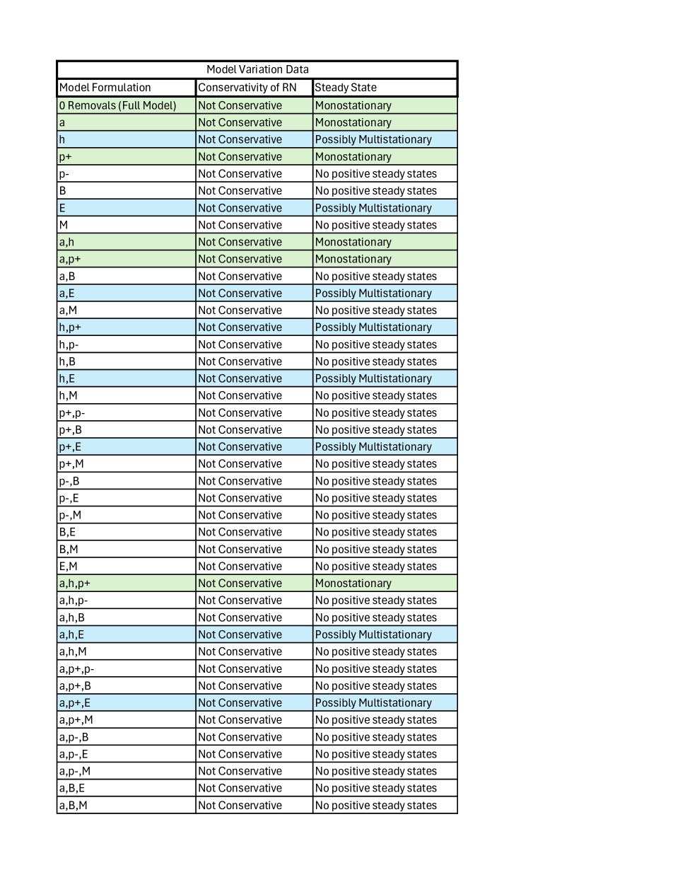
Figure 1: Steady state information for distinct subnetworks of the mass action gut microbiota model, Part 1 of 3.

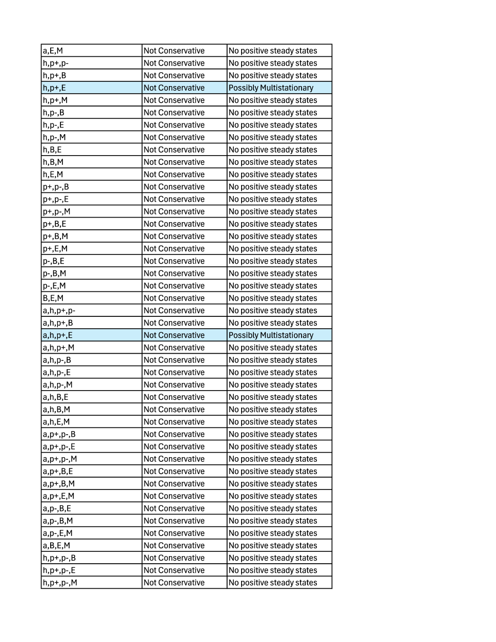
Figure 2: Steady state information for distinct subnetworks of the mass action gut microbiota model, Part 2 of 3.

Figure 3: Steady state information for distinct subnetworks of the mass action gut microbiota model, Part 3 of 3.

From this figure we can make a few observations regarding the removal of outflow reactions involving certain species. Removal of outflow reactions involving species $p-,B,M$ totally destroy the systems ability to obtain a single positive steady state. We can also note that removal of the outflow reaction involving species $E$ always gives rise to a subnetwork with the capacity for multistationarity. This highlights the influence that the rate constants for the outflow reactions involving $p-,B,M,E$ have on the number of steady states of this model.

Acknowledgements

The authors thank Prof. Colleen Mitchell and Prof. Zahra Aminzare for their insights, suggestions, and conversations. JMS thanks Prof. Elisenda Feliu and Prof. Alicia Dickenstein for their wonderful summer school through MSRI in Leipzig, and Skye Dore-Hall and José Lozano for their contributions to the examples in 38, 54.

References

- Adrian et al. [2023] Melissa A. Adrian, Bruce P. Ayati, and Ashutosh K. Mangalam. A mathematical model of bacteroides thetaiotaomicron, methanobrevibacter smithii, and eubacterium rectale interactions in the human gut. Scientific Reports, 13(1), Dec 2023. doi:10.1038/s41598-023-48524-4.
- Anderson [2008] David F. Anderson. Global asymptotic stability for a class of nonlinear chemical equations. SIAM Journal on Applied Mathematics, 68(5):1464–1476, Jan 2008. %****␣main.bbl␣Line␣25␣****doi:10.1137/070698282.
- Anderson and Shiu [2010] David F. Anderson and Anne Shiu. The dynamics of weakly reversible population processes near facets. SIAM Journal on Applied Mathematics, 70(6):1840–1858, Jan 2010. doi:10.1137/090764098.
- Bezanson et al. [2017] Jeff Bezanson, Alan Edelman, Stefan Karpinski, and Viral B Shah. Julia: A fresh approach to numerical computing. SIAM Review, 59(1):65–98, 2017. doi:10.1137/141000671. URL https://epubs.siam.org/doi/10.1137/141000671.
- Conradi et al. [2017] Carsten Conradi, Elisenda Feliu, Maya Mincheva, and Carsten Wiuf. Identifying parameter regions for multistationarity. PLOS Computational Biology, 13(10), 2017. %****␣main.bbl␣Line␣50␣****doi:10.1371/journal.pcbi.1005751.
- Craciun et al. [2008] Gheorghe Craciun, J. William Helton, and Ruth J. Williams. Homotopy methods for counting reaction network equilibria. Mathematical Biosciences, 216(2):140–149, 2008. doi:10.1016/j.mbs.2008.09.001.
- Decker et al. [2024] Wolfram Decker, Christian Eder, Claus Fieker, Max Horn, and Michael Joswig, editors. The Computer Algebra System OSCAR: Algorithms and Examples, volume 32 of Algorithms and Computation in Mathematics. Springer, 1 edition, 8 2024. URL https://link.springer.com/book/9783031621260.
- Dummit and Foote [2004] David Steven Dummit and Richard M. Foote. Abstract algebra. John Wiley & Sons, 2004.
- Eisenbud and Sturmfels [1996] David Eisenbud and Bernd Sturmfels. Binomial ideals. Duke Math. J., 84(1):1–45, July 1996.
- [10] Phillipp R. Ellison. PhD thesis.
- Feinberg [1972] Martin Feinberg. Complex balancing in general kinetic systems. Archive for Rational Mechanics and Analysis, 49(3):187–194, 1972. doi:10.1007/bf00255665.
- Feinberg [1995] Martin Feinberg. The existence and uniqueness of steady states for a class of chemical reaction networks. Archive for Rational Mechanics and Analysis, 132(4):311–370, 1995. doi:10.1007/bf00375614.
- Feinberg [2019] Martin Feinberg. Foundations of chemical reaction network theory. Springer, 2019.
- Feinberg et al. [2018] Martin Feinberg, Phillipp Ellison, Haixia Ji, and Daniel Knight. Chemical reaction network toolbox, Nov 2018. URL https://zenodo.org/records/5149266#.YSE_3d8pCUk.
- Gowda et al. [2021] Shashi Gowda, Yingbo Ma, Alessandro Cheli, Maja Gwozdz, Viral B Shah, Alan Edelman, and Christopher Rackauckas. High-performance symbolic-numerics via multiple dispatch. arXiv preprint arXiv:2105.03949, 2021.
- Gross et al. [2020] Elizabeth Gross, Heather Harrington, Nicolette Meshkat, and Anne Shiu. Joining and decomposing reaction networks. Journal of Mathematical Biology, 80(6):1683–1731, Mar 2020. %****␣main.bbl␣Line␣125␣****doi:10.1007/s00285-020-01477-y.
- Horn [1972] F. Horn. Necessary and sufficient conditions for complex balancing in chemical kinetics. Archive for Rational Mechanics and Analysis, 49(3):172–186, 1972. doi:10.1007/bf00255664.
- Horn and Jackson [1972] F. Horn and R. Jackson. General mass action kinetics. Archive for Rational Mechanics and Analysis, 47(2):81–116, Jan 1972. doi:10.1007/bf00251225.
- Ji [2011] Haixia Ji. PhD thesis, Ohio State University, 2011.
- Joshi and Shiu [2012] Badal Joshi and Anne Shiu. Simplifying the jacobian criterion for precluding multistationarity in chemical reaction networks. SIAM Journal on Applied Mathematics, 72(3):857–876, 2012. doi:10.1137/110837206.
- Ma et al. [2021] Yingbo Ma, Shashi Gowda, Ranjan Anantharaman, Chris Laughman, Viral Shah, and Chris Rackauckas. Modelingtoolkit: A composable graph transformation system for equation-based modeling, 2021.
- [22] OSCAR. Oscar – open source computer algebra research system, version 1.2.0-dev, 2024. URL https://www.oscar-system.org.
- [23] Igor Plazl and Polona Znidarsic-Plazl. Microbioreactors, page 289–301. Elsevier, third edition. URL https://www.sciencedirect.com/science/article/abs/pii/B9780128096338090713.
- Shiu and Sturmfels [2010] Anne Shiu and Bernd Sturmfels. Siphons in chemical reaction networks. Bulletin of Mathematical Biology, 72(6):1448–1463, Jan 2010. doi:10.1007/s11538-010-9502-y.
- Winder and Lanthaler [2011] Catherine L. Winder and Karin Lanthaler. Chapter fourteen - the use of continuous culture in systems biology investigations. In Daniel Jameson, Malkhey Verma, and Hans V. Westerhoff, editors, Methods in Systems Biology, volume 500 of Methods in Enzymology, pages 261–275. Academic Press, 2011. doi:https://doi.org/10.1016/B978-0-12-385118-5.00014-1. URL https://www.sciencedirect.com/science/article/pii/B9780123851185000141.