Split Gibbs Discrete Diffusion Posterior Sampling

Abstract

We study the problem of posterior sampling in discrete-state spaces using discrete diffusion models. While posterior sampling methods for continuous diffusion models have achieved remarkable progress, analogous methods for discrete diffusion models remain challenging. In this work, we introduce a principled plug-and-play discrete diffusion posterior sampling algorithm based on split Gibbs sampling, which we call SG-DPS. Our algorithm enables reward-guided generation and solving inverse problems in discrete-state spaces. We demonstrate that SG-DPS converges to the true posterior distribution on synthetic benchmarks, and enjoys state-of-the-art posterior sampling performance on a range of benchmarks for discrete data, achieving up to 2x improved performance compared to existing baselines.

1 Introduction

We study the problem of posterior sampling with discrete diffusion models. Given a pretrained discrete diffusion model (Sohl-Dickstein et al., 2015; Austin et al., 2021; Campbell et al., 2022; Lou et al., 2024) that models the prior distribution $p({\mathbf{x}})$, our goal is to sample from the posterior $p({\mathbf{x}}|{\mathbf{y}})$ in a plug-and-play fashion, where ${\mathbf{y}}$ represents a guiding signal of interest. This setting encompasses both solving inverse problems (e.g., if ${\mathbf{y}}$ is an incomplete measurement of ${\mathbf{x}}$), and conditional or guided generation (e.g., sampling from $p({\mathbf{x}})\exp(r({\mathbf{x}})/\alpha))/Z$ according to a reward function $r(\cdot)$).

Existing works on diffusion posterior sampling (Chung et al., 2023; Song et al., 2023a; Mardani et al., 2023; Wu et al., 2024) primarily focus on continuous diffusion models operating in the Euclidean space for ${\mathbf{x}}$. These methods have achieved remarkable success in applications including natural image restorations (Kawar et al., 2022; Chung et al., 2023; Zhu et al., 2023), medical imaging (Jalal et al., 2021; Song et al., 2022; Chung & Ye, 2022) and various scientific inverse problems (Feng et al., 2023; Wu et al., 2024; Zheng et al., 2024a). However, posterior sampling with discrete diffusion models in discrete-state spaces remains a challenging problem, mainly due to not having well-defined gradients of the likelihood function $p({\mathbf{y}}|{\mathbf{x}})$. Initial work to address this gap for discrete diffusion models relies on approximating value functions (similar to reinforcement learning) for derivative-free sampling (Li et al., 2024), which can be difficult to tune for good performance, particularly when the guidance ${\mathbf{y}}$ is complicated.

In this paper, we develop a rigorous plug-and-play method based on the principle of split Gibbs sampling (Vono et al., 2019), which we refer to as SG-DPS. Our method addresses the posterior sampling problem ${\mathbf{x}}\sim p({\mathbf{x}}|{\mathbf{y}})$ by introducing an auxiliary variable ${\mathbf{z}}$ along with a regularization potential function $D({\mathbf{x}},{\mathbf{z}};\rho)$ to relax the original problem. The relaxed formulation enables efficient sampling via Gibbs sampling, which alternates between a likelihood sampling step and a prior sampling step using a pretrained discrete diffusion model. As regularization increases, both variables ${\mathbf{x}}$ and ${\mathbf{z}}$ converge to the target posterior distribution.

We validate SG-DPS on diverse inverse problems and reward guided generation problems that involve discrete data. We demonstrate that SG-DPS converges to the true posterior distribution on synthetic data, that SG-DPS solves discrete inverse problems accurately and efficiently on discretized image data and monophonic music data, and that SG-DPS excels at reward-guided sampling on guided DNA generation. Our method demonstrates strong sampling quality in all experiments. For instance, we achieve an $8.36\ \mathrm{dB}$ improvement of PSNR values on an MNIST XOR task, over $2\times$ smaller Hellinger distance in music infilling, and $36\%$ higher average reward in guided DNA generation compared to existing methods.

2 Preliminaries

2.1 Discrete Diffusion Models

Diffusion models (Song & Ermon, 2019, 2020; Ho et al., 2020; Song et al., 2021; Karras et al., 2022, 2024) generate data ${\mathbf{x}}\in\mathcal{X}$ by reversing a predefined forward process. When $\mathcal{X}\in\mathbb{R}^{n}$ is a Euclidean space, the forward process is typically defined to be a stochastic differential equation (Karras et al., 2022):

$$\mathrm{d}{\mathbf{x}}_{t}=\sqrt{2\dot{\sigma}_{t}\sigma_{t}}\mathrm{d}{\mathbf{w}}_{t},$$ (1)

where ${\mathbf{w}}_{t}$ is a standard Wiener process and $\{\sigma_{t}\}_{t=0}^{T}$ is a predefined noise schedule. This diffusion process is reversible once the score function $s({\mathbf{x}}_{t},t):=\nabla_{{\mathbf{x}}_{t}}\log p({\mathbf{x}}_{t};\sigma_{t})$ is learned. Starting from ${\mathbf{x}}_{T}\sim\mathcal{N}(0,\sigma_{T}^{2}{\bm{I}})$, we generate data following the reverse SDE:

$$\mathrm{d}{\mathbf{x}}_{t}=-2\dot{\sigma}_{t}\sigma_{t}\nabla_{{\mathbf{x}}_{t}}\log p({\mathbf{x}}_{t};\sigma_{t})\mathrm{d}t+\sqrt{2\dot{\sigma}_{t}\sigma_{t}}\mathrm{d}{\mathbf{w}}_{t}.$$ (2)

Recent works on discrete diffusion models (Sohl-Dickstein et al., 2015; Austin et al., 2021; Campbell et al., 2022; Lou et al., 2024) extend score-based generative methods from modeling continuous distributions in Euclidean spaces to categorical distributions in discrete-state spaces. Specifically, when the data distribution lies in a finite support $\mathcal{X}=\{1,\dots,N\}$, one can evolve a family of categorical distributions $p_{t}$ over $\mathcal{X}$ following a continuous-time Markov chain over the discrete elements,

$$\frac{\mathrm{d}p_{t}}{\mathrm{d}t}={\bm{Q}}_{t}p_{t},$$ (3)

where $p_{0}=p_{\text{data}}$ and ${\bm{Q}}_{t}\in\mathbb{R}^{N\times N}$ are diffusion matrices with a simple stationary distribution. To reverse this continuous-time Markov chain, it suffices to learn the concrete score $s({\mathbf{x}};t):=[\frac{p_{t}(\tilde{\mathbf{x}})}{p_{t}({\mathbf{x}})}]_{\tilde{\mathbf{x}}\neq{\mathbf{x}}}$, as the reverse process is given by

$$\frac{\mathrm{d}p_{T-t}}{\mathrm{d}t}=\bar{\bm{Q}}_{T-t}p_{T-t},$$ (4)

with $\bar{\bm{Q}}_{t,\tilde{\mathbf{x}}{\mathbf{x}}}=\frac{p_{t}(\tilde{\mathbf{x}})}{p_{t}({\mathbf{x}})}{\bm{Q}}_{t,{\mathbf{x}}\tilde{\mathbf{x}}}$ and $\bar{\bm{Q}}_{t,{\mathbf{x}}{\mathbf{x}}}=-\sum_{\tilde{\mathbf{x}}\neq{\mathbf{x}}}\bar{\bm{Q}}_{t,\tilde{\mathbf{x}}{\mathbf{x}}}$.

For sequential data ${\mathbf{x}}\in\mathcal{X}^{D}$, there is $N^{D}$ number of states in total. Instead of constructing an exponentially large diffusion matrix, we choose a sparse matrix that only perturbs tokens independently, i.e.,

$${\bm{Q}}_{t}({\mathbf{x}},\tilde{\mathbf{x}})=\sum_{d=1}^{D}{\bm{Q}}_{t}^{d}({\mathbf{x}}_{d},\tilde{\mathbf{x}}_{d})\delta_{{\mathbf{x}}_{1:D\backslash d},\tilde{\mathbf{x}}_{1:D\backslash d}},$$ (5)

so that ${\bm{Q}}_{t}$ is nonzero only when the hamming distance between ${\mathbf{x}}$ and $\tilde{\mathbf{x}}$ is no more than 1.

Example: uniform kernel. An example of such diffusion matrices is

$${\bm{Q}}_{t}=\dot{\sigma}_{t}{\bm{Q}}^{\mathrm{uniform}}=\dot{\sigma}_{t}\left(\frac{1}{N}\mathbf{1}\mathbf{1}^{T}-{\bm{I}}\right),$$ (6)

where $\sigma_{t}$ is a predefined noise schedule with $\sigma_{0}=0$ and $\sigma_{T}=\sigma_{\max}$. This uniform kernel transfers any distribution to a uniform distribution as $\sigma\to\infty$. Moreover,

$$p_{t} =\exp(\int_{0}^{t}{\bm{Q}}_{\tau}\mathrm{d}\tau)p_{0}=\exp(\sigma_{t}{\bm{Q}}^{\mathrm{uniform}})p_{0}$$

$$=\Big{(}e^{-\sigma_{t}}{\bm{I}}+(1-e^{-\sigma_{t}})\frac{\mathbf{1}\mathbf{1}^{T}}{N}\Big{)}p_{0}.$$ (7)

When ${\mathbf{x}}\in\mathcal{X}^{D}$ is a sequence of length $D$,

$$p_{t}({\mathbf{x}}_{t}|{\mathbf{x}}_{0})\ \propto\ \beta_{t}^{d({\mathbf{x}}_{t},{\mathbf{x}}_{0})}(1-\beta_{t})^{D-d({\mathbf{x}}_{t},{\mathbf{x}}_{0})}.$$ (8)

$d(\cdot,\cdot)$ is the Hamming distance between two sequences, and $\beta_{t}=\frac{N-1}{N}(1-e^{-\sigma_{t}})$.

2.2 Diffusion Posterior Sampling Methods

Diffusion posterior sampling is a class of methods that draw samples from $p({\mathbf{x}}|{\mathbf{y}})\ \propto\ p({\mathbf{x}})p({\mathbf{y}}|{\mathbf{x}})$ using a diffusion model trained on the prior $p({\mathbf{x}})$. This technique has been applied in two settings with slightly different formulations: solving inverse problems and loss/reward guided generation.

The goal of inverse problems is to reconstruct the underlying data ${\mathbf{x}}_{0}$ from its measurements, which are modeled as ${\mathbf{y}}={\bm{G}}({\mathbf{x}}_{0})+{\mathbf{n}}$, where ${\bm{G}}$ is the forward model, and ${\mathbf{n}}$ denotes the measurement noise. In this case, the likelihood function is given by $p({\mathbf{y}}|{\mathbf{x}})=p_{{\mathbf{n}}}({\mathbf{y}}-{\bm{G}}({\mathbf{x}}))$, where $p_{\mathbf{n}}$ denotes the noise distribution.

On the other hand, reward-guided generation (Song et al., 2023b; Huang et al., 2024; Nisonoff et al., 2024) focuses on generating samples that achieve higher rewards according to a given reward function $r(\cdot)$. Here, the likelihood is modeled as $p({\mathbf{y}}|{\mathbf{x}})\ \propto\ \exp(r({\mathbf{x}})/\alpha)$, where $\alpha>0$ is a temperature parameter that controls the strength of reward weighting.

Existing diffusion posterior sampling methods leverage (continuous) diffusion models as plug-and-play priors and modifies Equation 2 to generate samples from the posterior distribution $p({\mathbf{x}}|{\mathbf{y}})\ \propto\ p({\mathbf{x}})p({\mathbf{y}}|{\mathbf{x}})$. These methods can be broadly classified into four categories (Daras et al., 2024; Zheng et al., 2024b).

Guidance-based methods (Chung et al., 2023; Song et al., 2023b, a; Kawar et al., 2022; Wang et al., 2023; Zheng et al., 2024a) perform posterior sampling by adding an additional likelihood score term $\nabla_{{\mathbf{x}}_{t}}\log p({\mathbf{y}}|{\mathbf{x}}_{t})$ to the score function in Equation 2, and modifies the reverse SDE as follows:

$$\mathrm{d}{\mathbf{x}}_{t} =-2\dot{\sigma}_{t}\sigma_{t}(\nabla_{{\mathbf{x}}_{t}}\log p({\mathbf{x}}_{t};\sigma_{t})+\nabla_{{\mathbf{x}}_{t}}\log p({\mathbf{y}}|{\mathbf{x}}_{t}))\mathrm{d}t$$

$$\hskip 130.0002pt+\sqrt{2\dot{\sigma}_{t}\sigma_{t}}\mathrm{d}{\mathbf{w}}_{t}.$$ (9)

The intractable likelihood score term is approximated with various assumptions. However, these methods cannot be directly applied to discrete posterior sampling problems, where $\log p({\mathbf{y}}|{\mathbf{x}})$ is defined only on a finite support.

Sequential Monte Carlo (SMC) methods sample batches of particles iteratively from a series of distributions, which converge to the posterior distribution in limit. This class of methods (Cardoso et al., 2024; Dou & Song, 2024) exploits the sequential diffusion sampling process to sample from the posterior distribution. Similar ideas have been applied in Li et al. (2024) for reward-guided generation using discrete diffusion models, which rely on approximating a soft value function at each iteration. We compare our method to this approach in our experiments.

Variational methods (Mardani et al., 2023; Feng et al., 2023) solve inverse problems by approximating the posterior distribution with a parameterized distribution $q_{\bm{\theta}}$ and optimizing its Kullback-Leibler (KL) divergence with respect to the posterior. However, how to extend these methods to discrete diffusion models remains largely unexplored.

Variable splitting methods (Wu et al., 2024; Zhang et al., 2024; Zhu et al., 2023; Song et al., 2024; Xu & Chi, 2024) decompose posterior sampling into two simpler alternating steps. A representative of this category is the split Gibbs sampler (see Section 3), where the variable ${\mathbf{x}}_{t}$ is split into two random variables that both eventually converge to the posterior distribution. These methods are primarily designed for continuous diffusion models with Gaussian kernels, leveraging Langevin dynamics or optimization in Euclidean space as subroutines. Murata et al. (2024) extends this category to VQ-diffusion models in the discrete latent space using the Gumbel-softmax reparameterization trick. However, this approach is limited to discrete latent spaces with an underlying continuous embedding due to its reliance on softmax dequantization. In this work, we generalize the split Gibbs sampler to posterior sampling in categorical data by further exploiting the unique properties of discrete diffusion models.

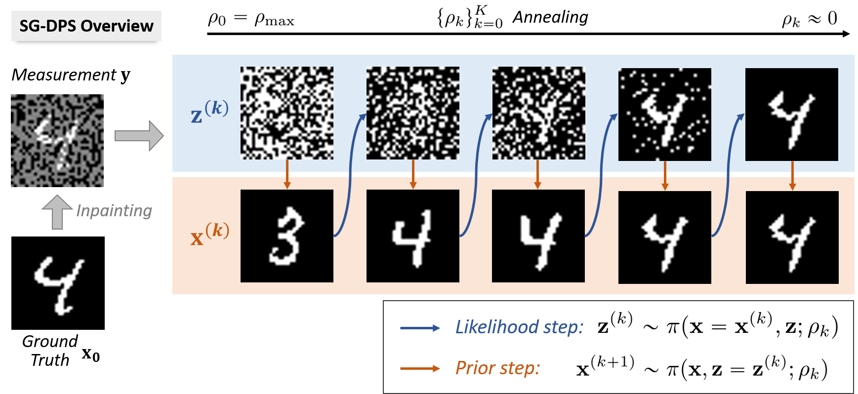
Figure 1: An illustration of our method on inpainting discretized MNIST. Our method implements the Split Gibbs sampler, which alternates between likelihood sampling steps and prior sampling steps. Likelihood sampling steps enforce data consistency with regard to measurement ${\mathbf{y}}$, while prior sampling steps involve denoising uniform noise from $z^{(k)}$ by a pretrained discrete diffusion model starting from noise level $\rho_{k}$. Two variables converge to a sample from the posterior distribution as the noise level $\rho_{k}$ reduces to zero.

3 Method

3.1 Split Gibbs for plug-and-play posterior sampling

Suppose we observe ${\mathbf{y}}$ from a likelihood function $p({\mathbf{y}}|{\mathbf{x}})$ and assume that ${\mathbf{x}}$ satisfies a prior distribution $p({\mathbf{x}})$. Our goal is to sample from the posterior distribution:

$$p({\mathbf{x}}|{\mathbf{y}})\ \propto\ p({\mathbf{y}}|{\mathbf{x}})p({\mathbf{x}})=\exp(-f({\mathbf{x}};{\mathbf{y}})-g({\mathbf{x}})),$$ (10)

where $f({\mathbf{x}};{\mathbf{y}})=-\log p({\mathbf{y}}|{\mathbf{x}})$ and $g({\mathbf{x}})=-\log p({\mathbf{x}})$. The challenge in sampling from this distribution arises from the interplay between the prior distribution, modeled by a diffusion model, and the likelihood function.

The Split Gibbs sampler (SGS) relaxes this sampling problem by introducing an auxiliary variable ${\mathbf{z}}$, allowing sampling from an augmented distribution:

$$\pi({\mathbf{x}},{\mathbf{z}};\rho)\ \propto\ \exp(-f({\mathbf{z}};{\mathbf{y}})-g({\mathbf{x}})-D({\mathbf{x}},{\mathbf{z}};\rho)),$$ (11)

where $D({\mathbf{x}},{\mathbf{z}};\rho)$ measures the distance between ${\mathbf{x}}$ and ${\mathbf{z}}$, and $\rho>0$ is a parameter that controls the strength of regularization. As $\rho\to 0$, $D({\mathbf{x}},{\mathbf{z}};\rho)\to\infty$ for any ${\mathbf{x}}\neq{\mathbf{z}}$, ensuring that both marginal distributions,

$$\pi^{X}({\mathbf{x}};\rho):=\int\pi({\mathbf{x}},{\mathbf{z}};\rho)\mathrm{d}{\mathbf{z}},\ \pi^{Z}({\mathbf{z}};\rho):=\int\pi({\mathbf{x}};{\mathbf{z}};\rho)\mathrm{d}{\mathbf{x}},$$ (12)

converges to the posterior distribution $p({\mathbf{x}}|{\mathbf{y}})$. The decoupling of the prior and likelihood in Equation 11 enables split Gibbs sampling, which alternates between two steps:

1. Likelihood sampling step:

$${\mathbf{z}}^{(k)}\sim\pi({\mathbf{x}}={\mathbf{x}}^{(k)},{\mathbf{z}};\rho)\ \propto\ \exp(-f({\mathbf{z}};{\mathbf{y}})-D({\mathbf{x}}^{(k)},{\mathbf{z}};\rho)),$$ (13)

2. Prior sampling step:

$${\mathbf{x}}^{(k+1)}\sim\pi({\mathbf{x}},{\mathbf{z}}={\mathbf{z}}^{(k)};\rho)\ \propto\ \exp(-g({\mathbf{x}})-D({\mathbf{x}},{\mathbf{z}}^{(k)};\rho)).$$ (14)

A key feature of split Gibbs sampling is that it does not rely on knowing gradients of the guidance term $f({\mathbf{z}};{\mathbf{y}})$, which is highly desirable in our setting with discrete data. In this way, split Gibbs is arguably the most natural and simplest framework for developing principled posterior sampling algorithms for discrete diffusion models.

Prior work has studied split Gibbs posterior sampling for continuous diffusion models (Coeurdoux et al., 2023; Wu et al., 2024; Xu & Chi, 2024). These methods specify the regularization potential as $D({\mathbf{x}},{\mathbf{z}};\rho)=-\frac{\|{\mathbf{x}}-{\mathbf{z}}\|_{2}^{2}}{2\rho^{2}}$, which transforms Equation 14 into a Gaussian denoising problem solvable by a diffusion model.

In the following sections, we explore how a specific choice of the potential $D({\mathbf{x}},{\mathbf{z}};\rho)$ links split Gibbs sampling to discrete diffusion models and discuss how the prior and likelihood sampling steps work in discrete-state spaces.

3.2 Prior Step with Discrete Diffusion Models

Suppose $p({\mathbf{x}})$ is a discrete-state distribution over $\mathcal{X}^{D}$ modeled by a diffusion process. We consider a discrete diffusion model with uniform transition kernel ${\bm{Q}}_{t}=\frac{1}{N}\mathbf{1}\mathbf{1}^{T}-{\bm{I}}$. We specify the potential function $D({\mathbf{x}};{\mathbf{z}};\rho)$ as:

$$D({\mathbf{x}},{\mathbf{z}};\rho):=d({\mathbf{x}},{\mathbf{z}})\log\frac{1+(N-1)e^{-\rho}}{(N-1)(1-e^{-\rho})},$$ (15)

where $d({\mathbf{x}},{\mathbf{z}})$ denotes the Hamming distance between ${\mathbf{x}}$ and ${\mathbf{z}}$. When $\rho\to 0^{+}$, the regularization potential $D({\mathbf{x}},{\mathbf{z}};\rho)$ goes to infinity unless $d({\mathbf{x}},{\mathbf{z}})=0$, ensuring the convergence of marginal distributions to $p({\mathbf{x}}|{\mathbf{y}})$. Given Equation 15, the prior step from Equation 14 is:

$${\mathbf{x}}^{(k+1)} \sim\pi({\mathbf{x}},{\mathbf{z}}={\mathbf{z}}^{(k)};\rho)$$

$$\ \propto\ p_{0}({\mathbf{x}})\left(\frac{\tilde{\beta}}{1-\tilde{\beta}}\right)^{d({\mathbf{z}}^{(k)},{\mathbf{x}})},$$ (16)

where $\tilde{\beta}=\frac{N-1}{N}(1-e^{-\rho})$. On the other hand, the distribution of clean data ${\mathbf{x}}_{0}$ conditioned on ${\mathbf{x}}_{t}$ is given by:

$$p({\mathbf{x}}_{0}|{\mathbf{x}}_{t}) \ \propto\ p_{0}({\mathbf{x}}_{0})p({\mathbf{x}}_{t}|{\mathbf{x}}_{0})$$

$$\ \propto\ p_{0}({\mathbf{x}}_{0})\beta_{t}^{d({\mathbf{x}}_{t},{\mathbf{x}}_{0})}(1-\beta_{t})^{D-d({\mathbf{x}}_{t},{\mathbf{x}}_{0})},$$ (17)

where $\beta_{t}=\frac{N-1}{N}(1-e^{-\sigma_{t}})$. Thus, sampling from Equation 16 is equivalent to unconditional generation from $p({\mathbf{x}}_{0}|{\mathbf{x}}_{t})$ when $\tilde{\beta}=\beta_{t}$, i.e., $\rho=\sigma_{t}$. Therefore, we can solve the prior sampling problem by simulating a partial discrete diffusion sampler starting from $\sigma_{t}=\rho$ and ${\mathbf{x}}_{t}={\mathbf{z}}^{(k)}$.

3.3 Likelihood Sampling Step

With the potential function $D({\mathbf{x}},{\mathbf{z}};\rho)$ specified in Section 3.2, at iteration $k$, the likelihood sampling step from Equation 13 can be written as:

$${\mathbf{z}}^{(k)} \sim\pi({\mathbf{x}}={\mathbf{x}}^{(k)},{\mathbf{z}};\rho)$$

$$\ \propto\ \exp\left(-f({\mathbf{z}};{\mathbf{y}})-d({\mathbf{x}},{\mathbf{z}})\log\frac{1+(N-1)e^{-\rho}}{(N-1)(1-e^{-\rho})}\right).$$ (18)

Since the unnormalized probability density function of $\pi({\mathbf{x}}={\mathbf{x}}^{(k)},{\mathbf{z}};\rho)$ is accessible, we can efficiently sample from Equation 18 using Markov Chain Monte Carlo methods. Specifically, we initialize ${\mathbf{z}}^{(k)}_{0}={\mathbf{x}}^{(k)}$ and run the Metropolis-Hasting algorithm to sample from Equation 18. The updating rule is given by:

$${\mathbf{z}}^{(k)}_{j+1}=\begin{cases}\tilde{\mathbf{z}}_{j},\quad\ \ \,\mathrm{w.p.}\ \alpha({\mathbf{z}}^{(k)}_{j}\to\tilde{\mathbf{z}}_{j}),\\ {\mathbf{z}}^{(k)}_{j},\quad\mathrm{otherwise},\end{cases}$$ (19)

where $\tilde{\mathbf{z}}_{j}$ is a proposal obtained by randomly flipping $s$ tokens in ${\mathbf{z}}^{(k)}_{j}$, and $\alpha({\mathbf{z}}^{(k)}_{j}\to\tilde{\mathbf{z}}_{j})$ denotes the acceptance probability of the proposal, given by:

$$\alpha({\mathbf{z}}^{(k)}_{j}\to\tilde{\mathbf{z}}_{j})=\min\left(1,\frac{\pi({\mathbf{x}}={\mathbf{x}}^{(k)},\tilde{\mathbf{z}}_{j};\rho)}{\pi({\mathbf{x}}={\mathbf{x}}^{(k)},{\mathbf{z}}^{(k)}_{j};\rho)}\right).$$ (20)

We repeat the Metropolis-Hastings update in Equation 19 for $T$ steps and set ${\mathbf{z}}^{(k)}={\mathbf{z}}^{(k)}_{T}$.

Algorithm 1 Split Gibbs Diffusion Posterior Sampling

 Require: Concrete score model ${\mathbf{s}}_{\theta}$, measurement ${\mathbf{y}}$, noise schedule $\{\rho_{k}\}_{k=0}^{K-1}$.

 Initialize ${\mathbf{x}}_{0}\in\mathcal{X}^{d}$

 for $k=0,\dots,K-1$ do

  Likelihood step following Equation 18

$${\mathbf{z}}^{(k)}\sim\pi({\mathbf{x}}={\mathbf{x}}^{(k)},{\mathbf{z}};\rho_{k}).$$

  Prior step following Equation 16.

$${\mathbf{x}}^{(k+1)}\sim\pi({\mathbf{x}},{\mathbf{z}}={\mathbf{z}}^{(k)};\rho_{k})$$

 end for

 Return ${\mathbf{x}}^{(K)}$

	$D=2$			$D=5$			$D=10$
	Hellinger $\downarrow$	TV $\downarrow$		Hellinger $\downarrow$	TV $\downarrow$		Hellinger $\downarrow$	TV $\downarrow$
SVDD-PM ($M=20$)	$0.297$	$0.320$		$0.413$	$0.458$		$0.455$	$0.503$
SVDD-PM ($M=100$)	$0.275$	$0.292$		$0.401$	$0.445$		$0.448$	$0.494$
DPS	$0.182$	$0.176$		$0.345$	$0.383$		$0.410$	$0.453$
SG-DPS	0.149	0.125		0.214	0.222		0.334	0.365

Table 1: Quantitative evaluation of posterior sampling on synthetic dataset for sequence lengths of $D=2,5$ and $10$. The Hellinger distance and total variance are computed between the empirical distribution of 10k samples and the true posterior distribution on the first two dimensions.

3.4 Overall Algorithm

We now summarize the complete SG-DPS algorithm. Like in Wu et al. (2024), our algorithm alternates between likelihood steps and prior steps while employing an annealing schedule $\{\rho_{k}\}$, which starts at a large $\rho_{0}$ and gradually decays to $\rho_{K}\to 0$. This annealing scheme accelerates the mixing time of the Markov chain and ensures the convergence of $\pi^{X}({\mathbf{x}};\rho)$ and $\pi^{Z}({\mathbf{z}};\rho)$ to $p({\mathbf{x}}|{\mathbf{y}})$ as $\rho\to 0$. Unlike prior work that uses uncontrolled approximations such as surrogate value functions,  SG-DPS does not rely on any approximation and eventually converges to the true posterior distribution. Consequently, SG-DPS can be viewed as a principled approach for posterior sampling using discrete diffusion models, leading to empirical benefits as shown in Section 4. We present the complete pseudocode of our method in Algorithm 1 and further explain the choice of the noise schedule in Section 4.6.

4 Experiments

We conduct experiments to demonstrate the effectiveness of our algorithm on various posterior sampling tasks in discrete-state spaces, including discrete inverse problems and reward/loss-guided generation.

4.1 Experimental Setup

We evaluate our method across multiple domains, including synthetic data, discrete image prior, monophonic music, and DNA sequences.

Pretrained models. For synthetic data, we use a closed-form concrete score function. For real datasets, we train a SEDD (Lou et al., 2024) model with the uniform transition kernel. These SEDD models are trained using AdamW (Loshchilov & Hutter, 2019) optimizer with a batch size of $32$ and a learning rate of $3\times 10^{-4}$.

Baselines. We compare our methods to existing approaches for discrete diffusion posterior sampling: DPS (Chung et al., 2023), SVDD (Li et al., 2024). SVDD is originally designed to sample from a reward-guided distribution $p^{\alpha}({\mathbf{x}})\ \propto\ p({\mathbf{x}})\exp(r({\mathbf{x}})/\alpha)$. To adapt it for posterior sampling, we let $r({\mathbf{x}})=\log p({\mathbf{y}}|{\mathbf{x}})$ and use a temperature of $\alpha=1$, so that $p^{\alpha}({\mathbf{x}})=p({\mathbf{x}}|{\mathbf{y}})$. DPS relies on gradient back-propagation through both the likelihood function and the pretrained diffusion model, making it unsuitable for discrete-domain posterior sampling. To adapt DPS for discrete diffusion models, we replace the gradient term $\nabla_{{\mathbf{x}}_{t}}\log p({\mathbf{y}}|{\mathbf{x}}_{t})$ with a guidance rate matrix ${\bm{R}}_{t}^{\mathbf{y}}=[\frac{p_{t}({\mathbf{y}}|\tilde{\mathbf{x}})}{p_{t}({\mathbf{y}}|{\mathbf{x}})}]_{{\mathbf{x}}\tilde{\mathbf{x}}}$, which is effectively a finite-difference approximation of a “discrete derivative”. Implementation details are provided in Section A.2.

SG-DPS implementation details. We implement our method with a total of $K=100$ iterations. In each prior sampling step, we simulate the reverse continuous-time Markov chain with $L=20$ steps. The likelihood function for inverse problems is defined as

$$p({\mathbf{y}}|{\mathbf{x}})\ \propto\ \exp(-\|{\bm{G}}({\mathbf{x}})-{\mathbf{y}}\|_{0}/\sigma_{{\mathbf{y}}}).$$ (21)

We set $\sigma_{{\mathbf{y}}}=0.1$ for most experiments. Additional details on hyperparameter choices are provided in Section A.3.

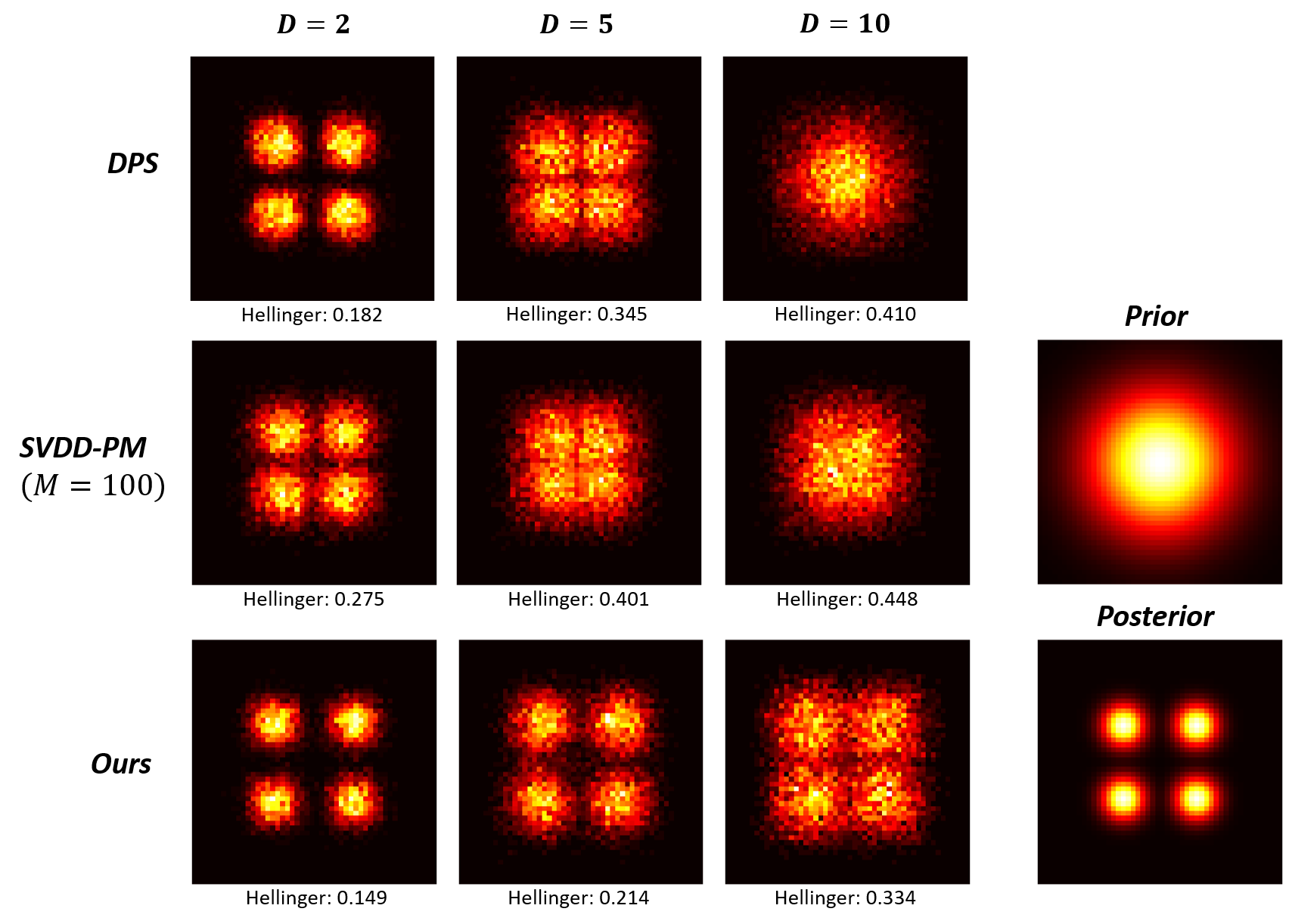
Figure 2: Empirical distributions of various sampling algorithms on the synthetic dataset. Heatmaps are drawn with 10k samples for sequence lengths of $D=2,5$ and $10$. We project the sequences to the first two dimensions for ease of visualization.

	XOR			AND
	PSNR $\uparrow$	Accuracy ($\%$) $\uparrow$		PSNR $\uparrow$	Accuracy ($\%$) $\uparrow$
SVDD-PM ($M=20$)	$11.81_{\pm 2.54}$	$51.4$		$10.04_{\pm 1.49}$	$33.7$
DPS	$9.04_{\pm 1.21}$	$30.0$		$8.67_{\pm 0.91}$	$24.5$
SG-DPS	$\textbf{20.17}_{\pm 3.47}$	91.2		$\textbf{17.25}_{\pm 3.82}$	79.4

Table 2: Quantitative results for XOR and AND problems on discretized MNIST. We report the mean and standard deviation of PSNR and class accuracy across 1k generated samples. The class accuracy is computed with a surrogate classifier trained on the training set. SG-DPS demonstrates superior performance on both tasks.

4.2 Controlled Study using Synthetic Data

We first evaluate the accuracy of SG-DPS in posterior sampling on a synthetic task where the true posterior distribution is accessible. Let ${\mathbf{x}}\in\mathcal{X}^{D}$ follow a prior distribution $p({\mathbf{x}})$, obtained by discretizing a Gaussian distribution $\mathcal{N}(0,\sigma^{2}{\bm{I}}_{D})$ over an $D$-dimensional grid. We define a forward model by ${\bm{G}}({\mathbf{x}})=\|f({\mathbf{x}})\|_{1}$ where $f({\mathbf{x}})$ maps ${\mathbf{x}}$ to $\mathbb{R}^{D}$, and likelihood function is defined as $p({\mathbf{y}}|{\mathbf{x}})\ \propto\ \exp(-|{\bm{G}}({\mathbf{x}})-{\mathbf{y}}|/\sigma_{\mathbf{y}}).$

Figure 3: Sampling results of the XOR task on the discretized MNIST dataset.  SG-DPS faithfully recovers the structural information of the ground truth signal.

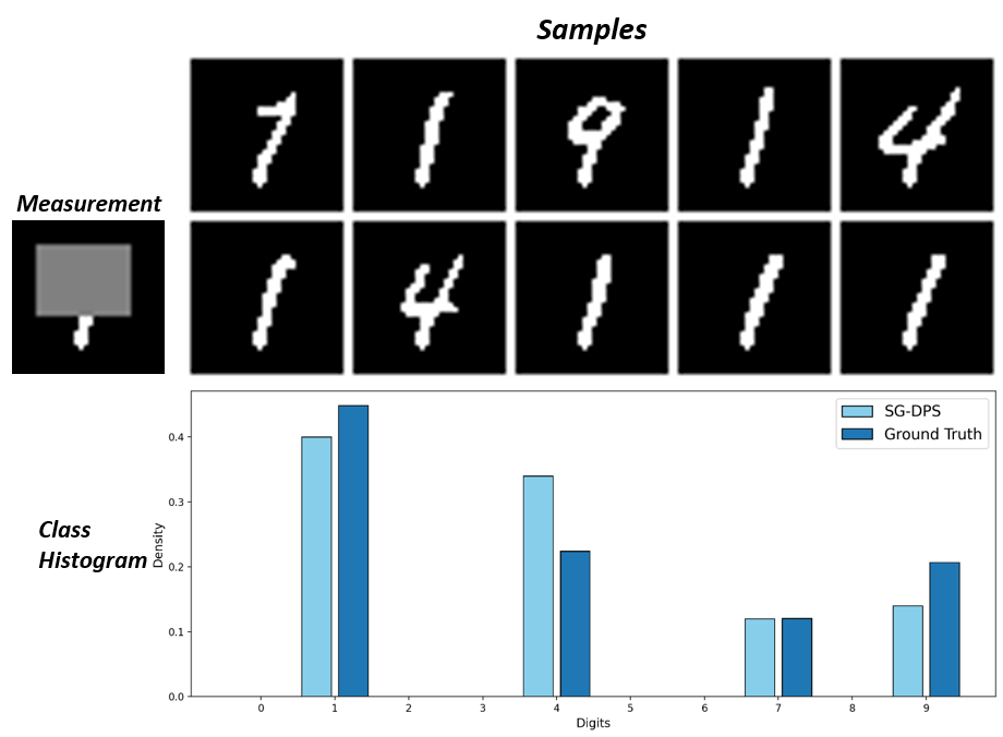
Figure 4: Diversified samples when the measurement ${\mathbf{y}}$ is sparse. We present 10 samples generated by SG-DPS when solving an MNIST inpainting task with sparse information. The class histogram is counted on 100 samples, showing SG-DPS generating digits of $1,4,7$ and $9$ that are consistent with the measurement. The ground truth distribution is calculated by counting all test samples with measurement error less than a threshold.

We choose $\sigma_{\mathbf{y}}=1$ specifically for synthetic data experiments. We draw 10k independent samples with each algorithm and compute the frequency map for the first two dimensions of ${\mathbf{x}}$. We measure the Hellinger distance and total variance distance between the empirical distribution and ground truth posterior distribution. As shown in Table 1, our method achieves substantially more accurate posterior sampling compared to baseline methods (by nearly a factor of 2x over SVDD-PM).

We visualize the generated samples in Figure 2 by projecting them onto the first two dimensions and computing their heatmaps. When the number of dimensions is small, e.g., $D=2$, all methods approximate the true posterior distribution well. However, as the dimensionality increases, DPS and SVDD-PM struggle to capture the posterior and tend to degenerate to the prior distribution. While SG-DPS consistently outperforms baseline methods in terms of Hellinger distance, it also shows a slight deviation from the posterior distribution as the dimensionality increases.

4.3 Discrete Image Inverse Problems

We evaluate on a discretized image domain. Specifically, we convert the MNIST dataset (LeCun et al., 1998) to binary strings by discretizing and flattening the images. We then train a discrete diffusion prior on 60k training data.

As examples of linear and nonlinear forward models on binary strings, we consider AND and XOR operators. We randomly pick $\gamma D$ pairs of positions $(i_{p},j_{p})$ over $\{1,\dots,D\}$, and compute:

$${\bm{G}}_{\mathrm{AND}}({\mathbf{x}})=[{\mathbf{x}}_{i_{p}}\wedge{\mathbf{x}}_{j_{p}}]_{p=1,\dots,\gamma D},$$

$${\bm{G}}_{\mathrm{XOR}}({\mathbf{x}})=[{\mathbf{x}}_{i_{p}}\oplus{\mathbf{x}}_{j_{p}}]_{p=1,\dots,\gamma D}.$$ (22)

These logical operators can be challenging to approximate using surrogate functions to guide diffusion sampling.

We assume $p({\mathbf{y}}|{\mathbf{x}})\ \propto\ \exp(-\|{\bm{G}}({\mathbf{x}})-{\mathbf{y}}\|_{0}/\sigma_{\mathbf{y}})$ for all experiments. We use 1000 binary images from the test set of MNIST and calculate the peak signal-to-noise ratio (PSNR) of the reconstructed image as a metric. Furthermore, we train a simple convolution neural network on MNIST as a surrogate and report the classifier accuracy of the generated samples. As shown in Table 2, SG-DPS outperforms baseline methods by a large margin in both XOR and AND tasks. We present the samples generated by SG-DPS for the XOR task in Figure 3. The reconstructed samples are visually consistent with the underlying ground truth signal, which explains the high class accuracy of our method shown in Table 2.

Sample diversity. Furthermore, we demonstrate that SG-DPS generates diversified samples when the measurement ${\mathbf{y}}$ is sparse. For example, when a digit is masked with a large box, as shown in Figure 4, the measurement lacks sufficient information to fully recover the original digit. In this scenario, SG-DPS generate samples from multiple plausible modes, including digits 1,4,7 and 9. This highlights the ability of our method to produce diverse samples from the posterior distribution while preserving consistency with the measurement.

4.4 Monophonic Music

We conduct experiments on monophonic songs from the Lakh pianoroll dataset (Dong et al., 2018). Following the preprocessing steps in (Campbell et al., 2022), we obtain monophonic musical sequences of length $D=256$ and vocabulary size $N=129$. The ordering of musical notes is scrambled to destroy any ordinal structure.

We evaluate our method on an inpainting task, where the forward model randomly masks $\gamma=60\%$ of the notes. As in (Campbell et al., 2022), we use the Hellinger distance of histograms and the proportion of outlier notes as metrics to evaluate our method. We run experiments on 100 samples in the test set and report the quantitative results in Table 3.  SG-DPS successfully completes monophonic music sequences in a style more consistent with the given conditions, achieving a 2x reduction in Hellinger distance compared to SVDD-PM.

	Hellinger $\downarrow$	Outliers $\downarrow$
SVDD-PM	$0.503_{\pm 0.134}$	$0.242_{\pm 0.184}$
SG-DPS	$\textbf{0.244}_{\pm 0.164}$	$\textbf{0.060}_{\pm 0.138}$

Table 3: Quantitative evaluation of infilling monophonic music sequences. We report the Hellinger distance between the histograms of generated samples and the ground truth.

4.5 Guided DNAs Generation

Following the setting in (Li et al., 2024), we evaluate on the guided generation of DNA sequences. This setting offers a natural real-world task for discrete diffusion models, and has been the focus of prior work on guided discrete diffusion.

We train a discrete diffusion model (Lou et al., 2024) on a dataset from Gosai et al. (2023). Here, we focus on sampling from a reward-guided distribution:

$$p^{\alpha}({\mathbf{x}})\ \propto\ p({\mathbf{x}})\exp(-r({\mathbf{x}})/\alpha).$$ (23)

meaning that the likelihood function is now defined as $p({\mathbf{y}}|{\mathbf{x}})=\exp(-r({\mathbf{x}})/\alpha)$. As in (Li et al., 2024), we use the Enformer model (Avsec et al., 2021) as the surrogate reward function $r(\cdot)$ to predict activity in the HepG2 cell line. We set $\alpha=0.1$ in our experiments.

We generate 100 DNA samples using different algorithms and compute the mean and median rewards of the generated sequences. As shown in Table 4, our method achieves the highest reward values compared to existing baselines, including 36% higher average reward compared to the previous state-of-the-art SVDD-PM method.

	Reward mean $\uparrow$	Reward median $\uparrow$
SVDD-PM	$5.24_{\pm 1.59}$	$5.21$
DPS	$1.85_{\pm 1.60}$	$1.42$
SG-DPS	$\textbf{7.13}_{\pm 1.83}$	6.93

Table 4: Quantitative results for guided DNA (enhancers) sampling. We generate 100 independent samples with different algorithms according to the reward-shaped posterior distribution. We report the mean and median of the enhancer’s activity computed by the surrogate reward.

4.6 Ablation Studies

Effectiveness of the annealing noise schedule. We now investigate how the choice of noise schedule $\{\rho_{k}\}_{k=0}^{K}$ affects the performance of SG-DPS. In our main experiments, we use a geometric noise schedule from (Lou et al., 2024), defined as $\rho_{k}=\rho_{\min}^{k/K}\rho_{\max}^{1-k/K}$. We argue that an annealing noise schedule $\{\rho_{k}\}_{k=0}^{K}$ that gradually decays to $\rho_{\min}\approx 0$ allows SG-DPS to converge faster and more accurately to the posterior distribution.

To validate this hypothesis, we conduct an ablation study on the MNIST AND task. We run our method for $K=50$ iterations and compare the annealing noise schedule with fixed noise schedules at different noise levels, ranging from $10^{-3}$ to $0.5$. We then compute the PSNR between ${\mathbf{x}}^{(k)}$ and the true underlying signal.

As shown in Figure 5, running SG-DPS with the annealing noise schedule achieves the highest PSNR and also the fastest convergence speed. Moreover, when $\rho$ is large, SG-DPS converges quickly to a poor solution, whereas when $\rho$ is small, it converges slowly to an accurate solution. This finding aligns with our intuition that SG-DPS is most accurate with $\rho\to 0$, while sampling with $\rho>0$ regularizes and simplifies the sampling problem.

This trade-off between convergence speed and accuracy results in a non-monotonic relationship between PSNR and fixed noise levels: PSNR first increases and then decreases with $\rho$. Therefore, using an annealing noise schedule helps provide both fast initial convergence and accurate posterior sampling as $\rho_{k}$ approaches 0.

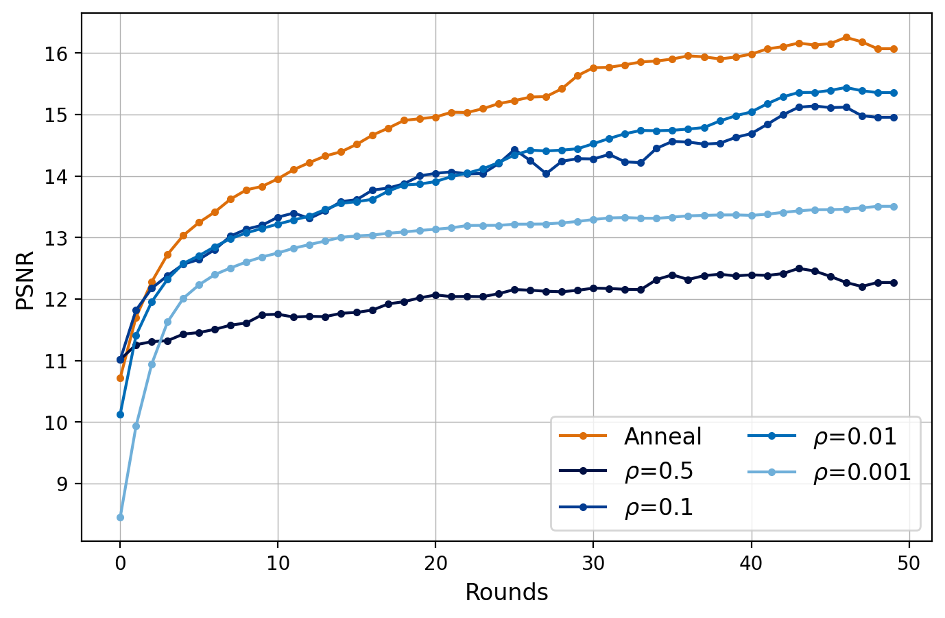
Figure 5: Convergence speed of different noise schedules. We compare our noise annealing scheduler $\{\rho_{k}\}_{k=1}^{K}$ (orange) to fixed noise schedules of various noise levels on the MNIST AND task. $y$-axis is the PSNR of variables ${\mathbf{x}}^{(k)}$ with respect to the ground truth. Our noise schedule converges faster than schedulers with fixed noises.

Time efficiency. We run SG-DPS with different configurations to evaluate its performance under different computing budgets. We control the number of iterations, $K$, and the number of unconditional sampling steps $T$ in each prior sampling step, so the number of function evaluations (NFE) of the discrete diffusion model is $KT$. We evaluate SG-DPS with NFE ranging from $100$ to $2$k. The detailed configuration is specified in Section B.1.

We present a plot in Figure 6 showing the tradeoff between sample quality and computing budgets in terms of NFEs.  SG-DPS is able to generate high-quality samples with a reasonable budget comparable to an unconditional generation.

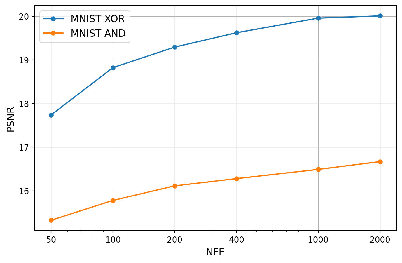
Figure 6: Sampling quality vs. computing budget. The $x$-axis indicates the number of function evaluations of the discrete diffusion, while the $y$-axis shows the PSNR metric. Experiments are done with 10 discretized MNIST samples on XOR and AND tasks.

Comparison to sampling without prior. We evaluate the value of discrete diffusion priors in solving discrete inverse problems by comparing our method to the Metropolis-Hasting algorithm without diffusion prior. We pick the AND problem on discretized MNIST as an example, in which we choose $\gamma D$ random pairs of pixels and compute their AND values as measurement ${\mathbf{y}}$. Figure 7 shows the reconstructed samples of SG-DPS and direct MCMC sampling under different levels of measurement sparsity. As demonstrated in the figure, the discrete diffusion model complements the missing information when the measurement is sparse (e.g., $\gamma=2,4,8$), underscoring the importance of discrete diffusion priors in SG-DPS for solving discrete inverse problems.

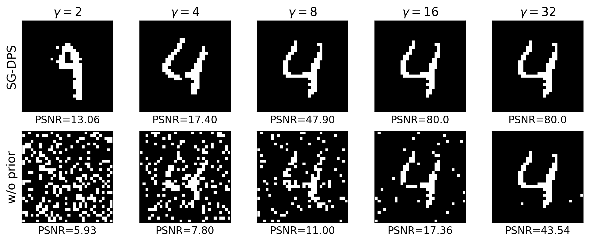
Figure 7: Comparison of SG-DPS and direct sampling without data prior. The PSNR values are computed with 10 test samples. SG-DPS replenishes the missing information when the measurement is sparse.

5 Conclusion

We introduce SG-DPS, a principled discrete diffusion posterior sampling algorithm based on the split Gibbs sampler, extending plug-and-play diffusion methods from Euclidean spaces to discrete-state spaces. Our algorithm iteratively alternates between prior and likelihood sampling steps with increasing regularization. By carefully designing the regularization potential function, we establish a connection between prior sampling steps and discrete diffusion samplers, integrating discrete diffusion models into the split Gibbs sampling framework. We evaluate our method on diverse tasks from various domains, including solving inverse problems and sequence generation guided by reward functions, where it significantly outperforms existing baselines.

Appendix A Experimental details

A.1 Pretrained Models

We learn prior distributions for each dataset using SEDD (Lou et al., 2024) discrete diffusion models. We use the SEDD small architecture with around 90M parameters for all experiments, and the models are trained with AdamW (Loshchilov & Hutter, 2019) with batch size $32$ and a learning rate of $3\times 10^{-4}$.

A.2 Baseline Methods

A.2.1 DPS

DPS (Chung et al., 2023) is designed to solve general inverse problems with a pretrained (continuous) diffusion model. It performs posterior sampling from $p({\mathbf{x}}|{\mathbf{y}})$ by modifying the reverse SDE

$$\mathrm{d}x_{t} =-2\dot{\sigma}_{t}\sigma_{t}\nabla_{{\mathbf{x}}_{t}}\log p({\mathbf{x}}_{t}|{\mathbf{y}})\mathrm{d}t+\sqrt{2\dot{\sigma}_{t}\sigma_{t}}\mathrm{d}t$$ (24)

$$=-2\dot{\sigma}_{t}\sigma_{t}(\nabla_{{\mathbf{x}}_{t}}\log p({\mathbf{x}}_{t};\sigma_{t}))+\nabla_{{\mathbf{x}}_{t}}\log p({\mathbf{y}}|{\mathbf{x}}_{t}))\mathrm{d}t+\sqrt{2\dot{\sigma}_{t}\sigma_{t}}\mathrm{d}t.$$ (25)

To estimate the intractable guidance term $\nabla_{{\mathbf{x}}_{t}}\log p({\mathbf{y}}|{\mathbf{x}}_{t})\mathrm{d}t$, DPS proposes to approximate it with $p({\mathbf{y}}|{\mathbf{x}}_{t})\approx p({\mathbf{y}}|\mathbb{E}[{\mathbf{x}}_{0}|{\mathbf{x}}_{t}])$. The guidance term is thus approximated by

$$\nabla_{{\mathbf{x}}_{t}}\log p({\mathbf{y}}|{\mathbf{x}}_{t})\approx-\nabla_{{\mathbf{x}}_{t}}\frac{\|{\bm{G}}({\bm{D}}_{\theta}({\mathbf{x}}_{t},\sigma_{t}))-{\mathbf{y}}\|_{2}^{2}}{2\sigma_{\mathbf{y}}^{2}},$$ (26)

where ${\bm{D}}_{\theta}$ is a one-step denoiser using the pretrained diffusion model, and the measurement is assumed to be ${\mathbf{y}}={\bm{G}}({\mathbf{x}})+{\mathbf{n}}$ with ${\mathbf{n}}\sim\mathcal{N}(0,\sigma_{{\mathbf{y}}}^{2}{\bm{I}})$.

However, DPS is not directly applicable to inverse problems in discrete-state spaces since propagating gradients through ${\bm{G}}$ and ${\bm{D}}_{\theta}$ in Equation 26 is impossible. Therefore, we consider the counterpart of DPS in discrete spaces. We modify the continuous-time Markov chain of the discrete diffusion model by

$$\frac{\mathrm{d}p_{T-t}}{\mathrm{d}t}=\tilde{\bm{Q}}_{T-t}p_{T-t},$$ (27)

in which

$$\tilde{\bm{Q}}_{t},\tilde{\mathbf{x}}{\mathbf{x}}=\frac{p_{t}(\tilde{\mathbf{x}}|{\mathbf{y}})}{p_{t}({\mathbf{x}}|{\mathbf{y}})}=\frac{p_{t}(\tilde{\mathbf{x}})}{p_{t}({\mathbf{x}})}\frac{p_{t}({\mathbf{y}}|\tilde{\mathbf{x}})}{p_{t}({\mathbf{y}}|{\mathbf{x}})}={\bm{Q}}_{t},\tilde{\mathbf{x}}{\mathbf{x}}\cdot\frac{p_{t}({\mathbf{y}}|\tilde{\mathbf{x}})}{p_{t}({\mathbf{y}}|{\mathbf{x}})}$$ (28)

Similar ideas are applied to classifier guidance for discrete diffusion models (Nisonoff et al., 2024), where the matrix ${\bm{R}}_{t}^{\mathbf{y}}=[\frac{p_{t}({\mathbf{y}}|\tilde{\mathbf{x}})}{p_{t}({\mathbf{y}}|{\mathbf{x}})}]_{{\mathbf{x}}\tilde{\mathbf{x}}}$ is called a guidance rate matrix. We compute ${\bm{R}}_{t}^{\mathbf{y}}$ at ${\mathbf{x}}$-column by enumerating every neighboring $\tilde{\mathbf{x}}$ and calculating $\frac{p_{t}({\mathbf{y}}|\tilde{\mathbf{x}})}{p_{t}({\mathbf{y}}|{\mathbf{x}})}$ for each $\tilde{\mathbf{x}}$. The discrete version of DPS can be summarized by

$$\frac{\mathrm{d}p_{T-t}}{\mathrm{d}t}=\bar{\bm{Q}}_{T-t}{\bm{R}}_{t}^{\mathbf{y}}p_{T-t}.$$ (29)

However, the discrete version of DPS is very time-consuming, especially when the vocabulary size is large, for it enumerates $(N-1)\times D$ number of neighboring $\tilde{x}$ when computing ${\bm{R}}_{t}^{\mathbf{y}}$. We find it slow for binary MNIST ($N=2$) and DNA generation tasks $(N=5)$ but unaffordable for monophonic music generation $(N=129)$.

A.2.2 SVDD

SVDD (Li et al., 2024) aims to sample from the distribution $p^{(\alpha)}({\mathbf{x}}_{0})\ \ \propto\ \ p({\mathbf{x}}_{0})\exp(r({\mathbf{x}}_{0})/\alpha)$, which is equivalent to the regularized MDP problem:

$$p^{(\alpha)}({\mathbf{x}}_{0})=\operatorname*{arg\,max}_{\pi}\mathbb{E}_{{\mathbf{x}}_{0}\sim\pi}r({\mathbf{x}}_{0})-\alpha\mathrm{KL}(p_{0}\|\pi)$$ (30)

They calculate the soft value function as

$$v_{t}({\mathbf{x}}_{t})=\alpha\log\mathbb{E}_{{\mathbf{x}}_{0}\sim p({\mathbf{x}}_{0}|{\mathbf{x}}_{t})}[\exp(r({\mathbf{x}}_{0})/\alpha)]$$ (31)

and propose to sample from the optimal policy

$$p_{t}^{\star}({\mathbf{x}}_{t}|{\mathbf{x}}_{t+1})\ \ \propto\ \ p_{t}({\mathbf{x}}_{t}|{\mathbf{x}}_{t+1})\exp(v_{t}({\mathbf{x}}_{t})/\alpha).$$ (32)

In time step $t$, SVDD samples a batch of $M$ particles from the unconditional distribution $p_{t}({\mathbf{x}}_{t}|{\mathbf{x}}_{t+1})$, and conduct importance sampling according to $\exp(v_{t}({\mathbf{x}}_{t})/\alpha)$.

Although (Li et al., 2024) is initially designed for guided diffusion generation; it also applies to solving inverse problems by carefully choosing reward functions. We consider $r({\mathbf{x}})=-\|{\bm{G}}({\mathbf{x}})-{\mathbf{y}}\|_{0}/\sigma_{\mathbf{y}}$ and $\alpha=1$, so that it samples from the posterior distribution $p({\mathbf{x}}|{\mathbf{y}})$. As recommended in (Li et al., 2024), we choose $\alpha=0$ in practice, so the importance sampling reduces to finding the particle with the maximal value in each iteration. We use SVDD-PM, a training-free method provided by (Li et al., 2024) in our experiments. It approximates the value function by $v_{t}({\mathbf{x}}_{t})=r(\hat{\mathbf{x}}_{0}({\mathbf{x}}_{t}))$, where $\hat{\mathbf{x}}_{0}({\mathbf{x}}_{t})$ is an approximation of $\mathbb{E}[{\mathbf{x}}_{0}|{\mathbf{x}}_{t}]$. In practice, we find that approximating $\hat{\mathbf{x}}_{0}({\mathbf{x}}_{t})$ by a few-step discrete sampler achieves slightly better results.

A.3 Hyperparameters

We use an annealing noise schedule of $\rho_{k}=\rho_{\min}^{k/K}\rho_{\max}^{1-k/K}$ with $\rho_{\min}=10^{-4}$ and $\rho_{\max}=20$. We run SG-DPS for $K$ iterations. In each likelihood sampling step, we run Metropolis-Hasting for $T$ steps, while in each prior sampling step, we run a few-step Euler discrete diffusion sampler with $L$ steps. The hyperparameters used for each experiment are listed in Table 5. We also include the dimension of data spaces $\mathcal{X}^{D}$ for each experiment in Table 5, where $|\mathcal{X}|=N$.

	Synthetic	MNIST XOR	MNIST AND	Music infilling	Guided DNA generation
$T$	10	2000	5000	5000	200
$K$	10	50	100	100	50
$L$	20	20	20	20	20
$D$	2/5/10	1024	1024	256	200
$N$	50	2	2	129	5

Table 5: Hyperparameters used in each experiment.

Appendix B Discussions

B.1 Sample Efficiency

We discuss the sampling efficiency of our method. The time cost of diffusion posterior sampling methods is closely related to the number of neural function evaluations (NFE) of the diffusion model. We present the detailed configurations of SG-DPS with different NFE budgets in Table 6. We report both the total NFE for the overall computation cost and the sequential NFE for the computation cost when each method is fully parallelized.

Configuration	$\#$ Iterations	Prior sampling steps	NFE	Runtime (sec/sample)
DPS	$100$	-	$102400/100$	820
SVDD-PM ($M=20$)	$128$	-	$2560/128$	16
SG-DPS-$50$	$25$	$2$	$50$	4
SG-DPS-$100$	$25$	$4$	$100$	6
SG-DPS-$200$	$40$	$5$	$200$	8
SG-DPS-$400$	$40$	$10$	$400$	10
SG-DPS-$1$k	$50$	$20$	$1000$	13
SG-DPS-$2$k	$100$	$20$	$2000$	20

Table 6: Configurations of SG-DPS and baseline methods. For DPS and SVDD-PM, we calculate both the total NFE and the sequential NFE. The numbers are collected from the MNIST XOR task as an example. The runtime is amortized on a batch size of 10 samples.

References

- Austin et al. (2021) Austin, J., Johnson, D. D., Ho, J., Tarlow, D., and Van Den Berg, R. Structured denoising diffusion models in discrete state-spaces. Advances in Neural Information Processing Systems, 34:17981–17993, 2021.
- Avsec et al. (2021) Avsec, Ž., Agarwal, V., Visentin, D., Ledsam, J. R., Grabska-Barwinska, A., Taylor, K. R., Assael, Y., Jumper, J., Kohli, P., and Kelley, D. R. Effective gene expression prediction from sequence by integrating long-range interactions. Nature methods, 18(10):1196–1203, 2021.
- Campbell et al. (2022) Campbell, A., Benton, J., De Bortoli, V., Rainforth, T., Deligiannidis, G., and Doucet, A. A continuous time framework for discrete denoising models. Advances in Neural Information Processing Systems, 35:28266–28279, 2022.
- Cardoso et al. (2024) Cardoso, G., el idrissi, Y. J., Corff, S. L., and Moulines, E. Monte carlo guided denoising diffusion models for bayesian linear inverse problems. In The Twelfth International Conference on Learning Representations, 2024. URL https://openreview.net/forum?id=nHESwXvxWK.
- Chung & Ye (2022) Chung, H. and Ye, J. C. Score-based diffusion models for accelerated mri. Medical Image Analysis, pp. 102479, 2022.
- Chung et al. (2023) Chung, H., Kim, J., Mccann, M. T., Klasky, M. L., and Ye, J. C. Diffusion posterior sampling for general noisy inverse problems. In The Eleventh International Conference on Learning Representations, 2023. URL https://openreview.net/forum?id=OnD9zGAGT0k.
- Coeurdoux et al. (2023) Coeurdoux, F., Dobigeon, N., and Chainais, P. Plug-and-play split gibbs sampler: embedding deep generative priors in bayesian inference. arXiv preprint arXiv:2304.11134, 2023.
- Daras et al. (2024) Daras, G., Chung, H., Lai, C.-H., Mitsufuji, Y., Ye, J. C., Milanfar, P., Dimakis, A. G., and Delbracio, M. A survey on diffusion models for inverse problems, 2024. URL https://arxiv.org/abs/2410.00083.
- Dong et al. (2018) Dong, H.-W., Hsiao, W.-Y., Yang, L.-C., and Yang, Y.-H. Musegan: Multi-track sequential generative adversarial networks for symbolic music generation and accompaniment. In Proceedings of the AAAI Conference on Artificial Intelligence, volume 32, 2018.
- Dou & Song (2024) Dou, Z. and Song, Y. Diffusion posterior sampling for linear inverse problem solving: A filtering perspective. In The Twelfth International Conference on Learning Representations, 2024. URL https://openreview.net/forum?id=tplXNcHZs1.
- Feng et al. (2023) Feng, B. T., Smith, J., Rubinstein, M., Chang, H., Bouman, K. L., and Freeman, W. T. Score-based diffusion models as principled priors for inverse imaging. In Proceedings of the IEEE/CVF International Conference on Computer Vision (ICCV), pp. 10520–10531, October 2023.
- Gosai et al. (2023) Gosai, S. J., Castro, R. I., Fuentes, N., Butts, J. C., Kales, S., Noche, R. R., Mouri, K., Sabeti, P. C., Reilly, S. K., and Tewhey, R. Machine-guided design of synthetic cell type-specific cis-regulatory elements. bioRxiv, 2023.
- Ho et al. (2020) Ho, J., Jain, A., and Abbeel, P. Denoising diffusion probabilistic models. In Larochelle, H., Ranzato, M., Hadsell, R., Balcan, M., and Lin, H. (eds.), Advances in Neural Information Processing Systems, volume 33, pp. 6840–6851. Curran Associates, Inc., 2020. URL https://proceedings.neurips.cc/paper_files/paper/2020/file/4c5bcfec8584af0d967f1ab10179ca4b-Paper.pdf.
- Huang et al. (2024) Huang, Y., Ghatare, A., Liu, Y., Hu, Z., Zhang, Q., Sastry, C. S., Gururani, S., Oore, S., and Yue, Y. Symbolic music generation with non-differentiable rule guided diffusion. arXiv preprint arXiv:2402.14285, 2024.
- Jalal et al. (2021) Jalal, A., Arvinte, M., Daras, G., Price, E., Dimakis, A. G., and Tamir, J. Robust compressed sensing mri with deep generative priors. In Ranzato, M., Beygelzimer, A., Dauphin, Y., Liang, P., and Vaughan, J. W. (eds.), Advances in Neural Information Processing Systems, volume 34, pp. 14938–14954. Curran Associates, Inc., 2021. URL https://proceedings.neurips.cc/paper_files/paper/2021/file/7d6044e95a16761171b130dcb476a43e-Paper.pdf.
- Karras et al. (2022) Karras, T., Aittala, M., Aila, T., and Laine, S. Elucidating the design space of diffusion-based generative models. In Oh, A. H., Agarwal, A., Belgrave, D., and Cho, K. (eds.), Advances in Neural Information Processing Systems, 2022. URL https://openreview.net/forum?id=k7FuTOWMOc7.
- Karras et al. (2024) Karras, T., Aittala, M., Lehtinen, J., Hellsten, J., Aila, T., and Laine, S. Analyzing and improving the training dynamics of diffusion models, 2024.
- Kawar et al. (2022) Kawar, B., Elad, M., Ermon, S., and Song, J. Denoising diffusion restoration models. In Advances in Neural Information Processing Systems, 2022.
- LeCun et al. (1998) LeCun, Y., Bottou, L., Bengio, Y., and Haffner, P. Gradient-based learning applied to document recognition. Proceedings of the IEEE, 86(11):2278–2324, 1998.
- Li et al. (2024) Li, X., Zhao, Y., Wang, C., Scalia, G., Eraslan, G., Nair, S., Biancalani, T., Ji, S., Regev, A., Levine, S., and Uehara, M. Derivative-free guidance in continuous and discrete diffusion models with soft value-based decoding, 2024. URL https://arxiv.org/abs/2408.08252.
- Loshchilov & Hutter (2019) Loshchilov, I. and Hutter, F. Decoupled weight decay regularization. In International Conference on Learning Representations, 2019. URL https://openreview.net/forum?id=Bkg6RiCqY7.
- Lou et al. (2024) Lou, A., Meng, C., and Ermon, S. Discrete diffusion modeling by estimating the ratios of the data distribution. In Forty-first International Conference on Machine Learning, 2024. URL https://openreview.net/forum?id=CNicRIVIPA.
- Mardani et al. (2023) Mardani, M., Song, J., Kautz, J., and Vahdat, A. A variational perspective on solving inverse problems with diffusion models. arXiv preprint arXiv:2305.04391, 2023.
- Murata et al. (2024) Murata, N., Lai, C.-H., Takida, Y., Uesaka, T., Nguyen, B., Ermon, S., and Mitsufuji, Y. G2d2: Gradient-guided discrete diffusion for image inverse problem solving, 2024. URL https://arxiv.org/abs/2410.14710.
- Nisonoff et al. (2024) Nisonoff, H., Xiong, J., Allenspach, S., and Listgarten, J. Unlocking guidance for discrete state-space diffusion and flow models, 2024. URL https://arxiv.org/abs/2406.01572.
- Sohl-Dickstein et al. (2015) Sohl-Dickstein, J., Weiss, E., Maheswaranathan, N., and Ganguli, S. Deep unsupervised learning using nonequilibrium thermodynamics. In International conference on machine learning, pp. 2256–2265. PMLR, 2015.
- Song et al. (2024) Song, B., Kwon, S. M., Zhang, Z., Hu, X., Qu, Q., and Shen, L. Solving inverse problems with latent diffusion models via hard data consistency. In The Twelfth International Conference on Learning Representations, 2024. URL https://openreview.net/forum?id=j8hdRqOUhN.
- Song et al. (2023a) Song, J., Vahdat, A., Mardani, M., and Kautz, J. Pseudoinverse-guided diffusion models for inverse problems. In International Conference on Learning Representations, 2023a. URL https://openreview.net/forum?id=9_gsMA8MRKQ.
- Song et al. (2023b) Song, J., Zhang, Q., Yin, H., Mardani, M., Liu, M.-Y., Kautz, J., Chen, Y., and Vahdat, A. Loss-guided diffusion models for plug-and-play controllable generation. In Krause, A., Brunskill, E., Cho, K., Engelhardt, B., Sabato, S., and Scarlett, J. (eds.), Proceedings of the 40th International Conference on Machine Learning, volume 202 of Proceedings of Machine Learning Research, pp. 32483–32498. PMLR, 23–29 Jul 2023b. URL https://proceedings.mlr.press/v202/song23k.html.
- Song & Ermon (2019) Song, Y. and Ermon, S. Generative modeling by estimating gradients of the data distribution. In Neural Information Processing Systems, 2019. URL https://api.semanticscholar.org/CorpusID:196470871.
- Song & Ermon (2020) Song, Y. and Ermon, S. Improved techniques for training score-based generative models. Advances in neural information processing systems, 33:12438–12448, 2020.
- Song et al. (2021) Song, Y., Sohl-Dickstein, J., Kingma, D. P., Kumar, A., Ermon, S., and Poole, B. Score-based generative modeling through stochastic differential equations. In International Conference on Learning Representations, 2021. URL https://openreview.net/forum?id=PxTIG12RRHS.
- Song et al. (2022) Song, Y., Shen, L., Xing, L., and Ermon, S. Solving inverse problems in medical imaging with score-based generative models. In International Conference on Learning Representations, 2022. URL https://openreview.net/forum?id=vaRCHVj0uGI.
- Vono et al. (2019) Vono, M., Dobigeon, N., and Chainais, P. Split-and-augmented gibbs sampler—application to large-scale inference problems. IEEE Transactions on Signal Processing, 67(6):1648–1661, 2019.
- Wang et al. (2023) Wang, Y., Yu, J., and Zhang, J. Zero-shot image restoration using denoising diffusion null-space model. In The Eleventh International Conference on Learning Representations, 2023. URL https://openreview.net/forum?id=mRieQgMtNTQ.
- Wu et al. (2024) Wu, Z., Sun, Y., Chen, Y., Zhang, B., Yue, Y., and Bouman, K. L. Principled probabilistic imaging using diffusion models as plug-and-play priors. arXiv preprint arXiv:2405.18782, 2024.
- Xu & Chi (2024) Xu, X. and Chi, Y. Provably robust score-based diffusion posterior sampling for plug-and-play image reconstruction. In The Thirty-eighth Annual Conference on Neural Information Processing Systems, 2024. URL https://openreview.net/forum?id=SLnsoaY4u1.
- Zhang et al. (2024) Zhang, B., Chu, W., Berner, J., Meng, C., Anandkumar, A., and Song, Y. Improving diffusion inverse problem solving with decoupled noise annealing, 2024. URL https://arxiv.org/abs/2407.01521.
- Zheng et al. (2024a) Zheng, H., Chu, W., Wang, A., Kovachki, N., Baptista, R., and Yue, Y. Ensemble kalman diffusion guidance: A derivative-free method for inverse problems, 2024a. URL https://arxiv.org/abs/2409.20175.
- Zheng et al. (2024b) Zheng, H., Chu, W., Zhang, B., Wu, Z., Wang, A., Feng, B., Zou, C., Sun, Y., Kovachki, N. B., Ross, Z. E., Bouman, K., and Yue, Y. Inversebench: Benchmarking plug-and-play diffusion models for scientific inverse problems. In Submitted to The Thirteenth International Conference on Learning Representations, 2024b. URL https://openreview.net/forum?id=U3PBITXNG6. under review.
- Zhu et al. (2023) Zhu, Y., Zhang, K., Liang, J., Cao, J., Wen, B., Timofte, R., and Gool, L. V. Denoising diffusion models for plug-and-play image restoration. In IEEE Conference on Computer Vision and Pattern Recognition Workshops (NTIRE), 2023.