Spectral theory of soliton gases for the defocusing NLS equation

Abstract

In this paper we derive Nonlinear Dispersion Relations (NDR) for the defocusing NLS (dark) soliton gas using the idea of thermodynamic limit of quasimomentum and quasienergy differentials on the underlying family of Riemann surfaces. It turns out that the obtained NDR are closely connected with the recently studied NDR for circular soliton gas for the focusing NLS. We find solutions for the kinetic equation for the defocusing NLS soliton condensate, which is defined by the endpoints of the spectral support $\Gamma$ for the NDR.It turns out that, similarly to KdV soliton condensates ([6]), the evolution of these endpoints is governed by the defocusing NLS-Whitham equations ([17]). We also study the Riemann problem for step initial data and the kurtosis of genus zero and one defNLS condensates, where we proved that the kurtosis of genus one condensate can not exceed 3/2, whereas for genus zero condensate the kurtosis is always 1.

1 Introduction

Spectral theory of soliton gases can be traced back to the paper of V. Zakharov [26], where the effective average velocity of a Korteweg-de Vries (KdV) soliton on the background of many other solitons was first derived. As it is well known, two such solitons moving with different velocities retain their shapes and velocities after the interaction but experience a phase shift. That is, the result of this interaction can be viewed as an “abrupt” shift of location of the center of each soliton involved. Naturally, the summary effect of consistent interactions changes the average velocity of a soliton, and that average velocity was derived in [26]. This property of soliton interactions is, to some extend, common for many integrable equations. It allows one to interpret ensembles of, say, KdV solitons as particles of some gas with a prescribed law of pairwise interactions. We will call it a KdV soliton gas.

In terms of the current KdV soliton gas theory, V. Zakharov’s formula described the average velocity of a soliton in the diluted KdV soliton gas. Here the word “diluted” means that solitons are so sparse that it is possible to distinguish individual soliton-soliton interactions or, in other words, that the spatial density of solitons is small. A successful attempt to derive the average velocity in the dense KdV soliton gas, pioneered by G. El in [10], was based on the idea of thermodynamic limit of finite-gap or nonlinear multiphase solutions to KdV. Multiphase KdV solutions are spectrally characterized by a finite numbers of segments (bands) on the spectral line ${\mathbb{R}}$, where each band corresponds to a particular mode. If one fixes the center of each band and starts to shrink these bands to their centers, one obtains in the limit a finite set of points (centers) on ${\mathbb{R}}$ that spectrally characterize a multi-soliton solution (each spectral point corresponds to a soliton). The wavenumbers and frequencies of nonlinear $N$-phase solutions can be described through the periods of the quasimomentum and quasienergy meromorphic differentials on the hyperelliptic Riemann surface(RS) $\mathcal{R}_{N}$, defined by the endpoints of the bands. In particular, the branchcuts of $\mathcal{R}_{N}$ consist of all the bands together with an additional branchcut going to $\infty$. The idea of thermodynamic limit is to increase the number $N$ of modes (bands) while simultaneously shrinking the size of each spectral band at a certain special rate. In the limit, the centers of spectral bands will be distributed at a some compact $\Gamma\subset{\mathbb{R}}$ with some positive probability density function $\phi(z)$. $\Gamma$ is usually assumed to be a finite set of segments sometimes referred to as superbands.

A soliton is uniquely defined by its spectral data, that is, by some $z\in{\mathbb{R}}$ and a real norming constant $c$. The value of $z$ does not change in the process of time $t$ evolution of the soliton whereas $c$ is multiplied by a factor $e^{8tz^{\frac{3}{2}}}$. At the same time, a nonlinear multiphase solution is defined by its collection of bands together with a real phase associated with each band. Like in the soliton case, the bands do not evolve with $t$ whereas phases undergo $t$ evolution similar to that of the norming constants. Existence of the thermodynamic limit of nonlinear multiphase solutions is generically not clear. However, under the right scaling of the bands (with $N$) one can expect the existence of continualized limits of wavenumbers and frequencies of these solutions, called density of states (DOS) $u(z)$ and density of fluxes (DOF) $v(z)$ respectively. In fact, the DOS and DOF were introduced in [10] as solutions of some Fredholm type integral equations. These equations form nonlinear dispersion relations (NDR) for the corresponding soliton gas, as they connect the $u$ and $v$ through the underlying thermodynamic limit of meromorphic differentials on RS $\mathcal{R}_{N}$. It is interesting to mention that the kernel of the integral operator in the NDR coincides with the phase shift expression for two interacting solitons.

The ratio $s(z)=\frac{v(z)}{u(z)}$ represents the average velocity of the element of the soliton gas parameterized by $z$. By replacing $v$ by $s$ and combining the two NDR, one can obtain a single integral equation connecting $u$ and $s$, called the equation of states. This equation ([10]) is a direct generalization of Zakharov’s average velocity expression from [26] to a dense soliton gas.

So far we described the homogeneous KdV soliton gas, that is, the case when $u,v$, as well as the spectral support $\Gamma$ does not depend on $x,t$. Assuming such dependence on very large scales, one comes to the idea of nonhomogeneous soliton gas, in which case the equation of states is complemented by conservation equation $u_{t}+v_{x}=0$. These two equations together are called kinetic equation, see [10].

The NLS equation has the form

$$i\psi_{t}+\psi_{xx}+2s|\psi|^{2}\psi=0,$$ (1.1)

where $x,t\in{\mathbb{R}}$ are the space-time variables, $s=\pm 1$ and $\psi:{\mathbb{R}}^{2}\rightarrow{\mathbb{C}}$ is the unknown complex-valued function. This equation describes the evolution of a slowly varying envelope of a quasi-monochromatic wave packet propagating through a focusing ($s=1$) or defocusing ($s=-1$) dispersive nonlinear medium.

The NDR and the kinetic equation for the focusing NLS (fNLS) soliton gases were derived in [11]. The main distinctions from the KdV case is that the fNLS solutions, including soliton solutions, are complex valued and are spectrally characterized by Schwarz symmetric sets in the ${\mathbb{C}}$. For example, a solitary wave (soliton) is spectrally represented by a pair of complex conjugated points $z,\bar{z}$, where $2|\operatorname{Im}z|$ represent the amplitude of the soliton and $-4\operatorname{Re}z$ represents its velocity. Therefore, the spectral support set $\Gamma$ is s Schwarz symmetrical set in ${\mathbb{C}}$, and the integral equations forming the NDR are complex valued. Below, we very briefly describe the construction of the NDR for fNLS, starting with a genus $N$ Schwarz symmetrical hyperelliptic Riemann surface $\mathcal{R}_{N}$.

The wavenumbers $k_{j}$ and frequencies $\omega_{j}$ of any finite gap solution to the fNLS, associated with $\mathcal{R}_{N}$, are defined in terms of $\mathcal{R}_{N}$. In particular, let $dp_{N}$, $dq_{N}$ be the second kind real normalized meromorphic differentials on $\mathcal{R}_{N}$ with poles only at infinity (both sheets) and with the principle parts $\pm 1$ for $dp_{N}$ and $\pm 2z$ for $dq_{N}$ there respectively. Here $z\in\mathcal{R}_{N}$ denotes the spectral parameter. and real normalized mean that all all the periods of $dp_{N}$, $dq_{N}$ on $\mathcal{R}_{N}$ are real. Then the vectors $\vec{k}$, $\vec{\omega}$ of the (real) periods of $dp_{N}$, $dq_{N}$ with respect to a fixed homology basis ($\bf A$ and $\bf B$ cycles) of $\mathcal{R}_{N}$ are vectors of the wavenumbers and frequencies of finite gap solutions on $\mathcal{R}_{N}$ respectively, i.e.,

$$k_{j}=\oint_{\bf A_{j}}dp_{N},~~~\tilde{k}_{j}=\oint_{\bf B_{j}}dp_{N},\quad\omega_{j}=\oint_{\bf A_{j}}dq_{N},~~~\tilde{\omega}_{j}=\oint_{\bf B_{j}}dq_{N},$$ (1.2)

where $\vec{k}=(k_{1},\dots,k_{N},\tilde{k}_{1},\dots,\tilde{k}_{N}),$ $\vec{\omega}=(\omega_{1},\dots,\omega_{N},\tilde{\omega}_{1},\dots,\tilde{\omega}_{N})$. The differentials $dp_{N}$, $dq_{N}$ are known as quasimomentum and quasienergy differentials respectively ( [13]).

Denote by $w_{j,N}=w_{j}$ the j-th normalized holomorphic differential on $\mathcal{R}_{N}$, $j=1,\dots,N$, that are defined by the condition $\int_{A_{k}}w_{j}=\delta_{k,j}$, $k=1,\dots,N$, where $\delta_{k,j}$ is the Kronecker delta. The well known Riemann Bilinear Relations (RBR)

$$\sum_{j}\left[\oint_{\bf A_{j}}w_{m}\oint_{\bf B_{j}}dp_{N}-\oint_{\bf A_{j}}dp_{N}\oint_{\bf B_{j}}w_{m}\right]=2\pi i{\sum}{\rm Res}(\int w_{m}dp_{N}),$$ (1.3)

$$\sum_{j}\left[\oint_{\bf A_{j}}w_{m}\oint_{\bf B_{j}}dq_{N}-\oint_{\bf A_{j}}dq_{N}\oint_{\bf B_{j}}w_{m}\right]=2\pi i{\sum}{\rm Res}(\int w_{m}dq_{N}),$$ (1.4)

$m=1,\dots,N$, form systems of linear equations for $\vec{k}$, $\vec{\omega}$ respectively, where the summation in the right hand side is taking over the only poles $z=\infty_{\pm}$ (infinities on both sheets of $\mathcal{R}_{N}$) of $dp_{N},dq_{N}$. Taking imaginary and real parts of (1.3), one gets

$$\sum_{j}k_{j}\operatorname{Im}\oint_{\bf B_{j}}w_{m}=-2\pi\operatorname{Re}\left(\sum{\rm Res}(\int w_{m}dp_{N})\right),$$ (1.5)

$$\tilde{k}_{m}=\sum_{j}k_{j}\operatorname{Re}\oint_{\bf B_{j}}w_{m}-2\pi\operatorname{Im}\left(\sum{\rm Res}(\int w_{m}dp_{N})\right),$$ (1.6)

$m=1,\dots,N$, respectively for (1.3). Similarly, we can calculate the imaginary and real parts of (1.4). We observe that the matrix of the $N\times N$ system of linear equations (1.5) is positive definite, since it is the imaginary part $\operatorname{Im}\tau$ of the Riemann period matrix $\tau=\oint_{\bf B_{j}}w_{m}$. Once $k_{j}$ are known, the values of $\tilde{k}_{j}$ can be calculated from (1.6). Thus, the systems (1.5)- (1.6) always have a unique solution. Similar results are true for (1.4). As the wavenumber and frequency vectors $\vec{k}$, $\vec{\omega}$ are connected via the underlying Riemann surface $\mathcal{R}_{N}$, we can interpret the RBR (1.3)- (1.4) as a (discrete) NDR for the finite gap solutions to the fNLS that are defined by $\mathcal{R}_{N}$.

One of the main subjects of the spectral theory of soliton gases is the thermodynamic limit of scaled vectors $\vec{k}$, $\vec{\omega}$, i.e., the thermodynamic limit of the RBR (1.3)-(1.4), which leads to a continualized version of the NDR established in [11], see equations (1.7)-(1.8) and (1.9)-(1.10) below.

The connection between a finite gap and a soliton solution can be illustrated on the example of an elliptic solution $\psi_{m}(x,t)=e^{it(2-m)}{\rm dn}(x,m)$ to the fNLS (1.1), where $\rm dn$ denotes the corresponding Jacobi elliptic function and $m\in[0,1]$ is the elliptic parameter. Spectrally, this solution is represented by two symmetric bands $\Gamma^{\pm}\subset[-i,i]$, whose endpoints depend on $m$. In fact $\Gamma^{+}=\frac{i}{2}[1-\sqrt{1-m},1+\sqrt{1-m}]$, where $\sqrt{1-m},1$ are the minimum and the maximum values of $\rm dn(x,m)$ on $x\in{\mathbb{R}}$ respectively. In the limit $m=0$ we obtain the plane wave $\psi_{0}(x,t)=e^{2it}$ with the spectral support $\Gamma^{+}=[0,i]$ In the opposite limit we obtain the soliton solution $\psi_{1}(x,t)=e^{it}\hbox{sech}(x)$ with the spectral support $\Gamma^{+}=\{\frac{1}{2}i\}$. That is, the period of an elliptic solution tends to infinity if one shrinks the spectral bands $\Gamma^{\pm}$ of this solution. Clearly, the corresponding wavenumber tends to zero.

For simplicity of describing the thermodynamic limit, let us assume that $N$ is even and only one (Schwarz symmetrical) band $\gamma_{0}$ intersects ${\mathbb{R}}$. We choose the $\bf A$ cycles as closed loops around every band except $\gamma_{0}$. Then the $\bf B$ cycle $\bf B_{j}$ is represented by a properly oriented loop going through the branch cut encircled by $\bf A_{j}$ and through the exceptional branch cut $\gamma_{0}$, $j=1,\dots,N$.

In the thermodynamic limit, we assume (see [11]) that the number $N+1$ of bands (the branch cuts of $\mathcal{R}_{N}$) is growing so that in the limit the centers of bands are distributed on some (Schwarz symmetrical) compact $\Gamma$ in ${\mathbb{C}}$ with a normalized continuous (Schwarz symmetrical) density $\phi(z)>0$, that is, $\int_{\Gamma^{+}}\phi(w)|dw|=1$, where on $\Gamma^{+}=\Gamma\cap{\mathbb{C}}^{+}$.

Simultaneously, the bandwidth of each band (except, possibly, $\gamma_{0}$) centered at $z\in\Gamma^{+}$ is shrinking at the order $e^{-\nu(z)N}$, where $\nu(z)$ is a continuous non-negative function on $\Gamma^{+}$, in such a way that the distance between any two bands should be of the order at least $O(1/N)$. The wavenumbers $k_{j}$ and frequencies $\omega_{j}$ are called solitonic wavenumbers and frequencies respectively, because in the thermodynamic limit they go to zero. The remaining quantities $\tilde{k}_{j},\tilde{\omega}_{j}$ from (1.2) are called carrier wavenumbers and frequencies respectively. The function ${\sigma}(z)=\frac{2\nu(z)}{\phi(z)}$ is called spectral scaling function. In the thermodynamic limit, the system of linear equations (1.5) for the solitonic wavenumbers $k_{j}$, subject to additional assumption that the size of the exceptional band $\gamma_{0}$ is also shrinking, turns into the integral equation (1.7) for the scaled continualized limit $u(z)$ of $k_{j}$:

$$\int_{\Gamma^{+}}\log\left|\frac{z-\bar{w}}{z-w}\right|u(w)|dw|+\sigma(z)u(z) =\operatorname{Im}{z},\quad z\in\Gamma^{+},$$ (1.7)

$$\int_{\Gamma^{+}}\log\left|\frac{z-\bar{w}}{z-w}\right|v(w)||dw|+\sigma(z)v(z) =-4\operatorname{Re}{z}\operatorname{Im}{z},\quad z\in\Gamma^{+}.$$ (1.8)

Similarly, the imaginary part of (1.4) for the solitonic frequencies $\omega_{j}$ turns into the integral equation (1.8) for the scaled continualized limit $v(z)$ of $\omega_{j}$. Thus, equations (1.7)-(1.8) represent the thermodynamic limit of the systems of linear equations for $k_{j},\omega_{j}$, i.e., the thermodynamic limit of imaginary parts of the RBR (1.3)-(1.4). They form the NDR for fNLS soliton gas. If we require that the exceptional band $\gamma_{0}$ stays unchanged, say, $\gamma_{0}=[-\delta_{0},\delta_{0}]$, $\delta_{0}\in i{\mathbb{R}}^{+}$, the thermodynamic limit will correspond to the fNLS breather gas. The NDR for the solitonic component of the fNLS breather gas have the form ([11])

$$\int_{\Gamma^{+}}\left[\log\left|\frac{w-\bar{z}}{w-z}\right|+\log\left|\frac{R_{0}(z)R_{0}(w)+zw-\delta_{0}^{2}}{R_{0}(\bar{z})R_{0}(w)+\bar{z}w-\delta_{0}^{2}}\right|\right]u(w)|dw|+\sigma(z)u(z)\\ =\operatorname{Im}R_{0}(z),$$ (1.9)

$$\int_{\Gamma^{+}}\left[\log\left|\frac{w-\bar{z}}{w-z}\right|+\log\left|\frac{R_{0}(z)R_{0}(w)+zw-\delta_{0}^{2}}{R_{0}(\bar{z})R_{0}(w)+\bar{z}w-\delta_{0}^{2}}\right|\right]v(w)|dw|+\sigma(z)v(z)\\ =-2\operatorname{Im}[zR_{0}(z)],$$ (1.10)

where $z\in\Gamma^{+}$ and $R_{0}(z)=\sqrt{z^{2}-\delta_{0}^{2}}$ with the branchcut $\gamma_{0}=[-\delta_{0},\delta_{0}]\subset i{\mathbb{R}}$.

Remark 1.1.

An interesting observation for both KdV ([10]) and fNLS ([11]) soliton gases is that the kernel of the integral operator of the 1st NDR divided by its the right hand side, i.e., $\frac{1}{\operatorname{Im}z}\log\left|\frac{z-\bar{w}}{z-w}\right|$ for equation (1.7), represents the well known phase shift formula of two interacting solitons with the corresponding spectral parameters $z,w$, see [27]. In fact, this observation can be extended to phase shifts of interacting breathers and the 1st NDR (1.9) for fNLS breather gases([11], [20]). In Remark 2.2, Section 2 we expand this observation to the defocusing NLS (defNLS) soliton gases and phase shifts of interacting dark solitons.

In the present paper we derive the NDR (Section 2) and the kinetic equation (Section 5) for the defNLS soliton gases, where the solitons are dark (depression) solitons on the plane wave background. The kernel of the integral operator in the obtained NDR, see (2.12)-(2.13), resemble that of the NDR (1.9)- (1.10) for the fNLS breather gas, if we anti Schwarz symmetrically extend $u(z),v(z)$ there to the lower half plane and integrate over $\Gamma=\Gamma^{+}\cup\overline{\Gamma^{+}}$. In Section 3 we show that the NDR (2.12)-(2.13) for the defNLS soliton gas can be transformed into the NDR for the circular fNLS soliton gas, which was studied in recent paper [24] of the authors. We remind that an fNLS soliton gas is called circular if $\Gamma^{+}$ is restricted to the upper semicircle $|z|=\rho$ for some $\rho>0$. Existence and uniqueness of solutions $u(z),v(z)$ to the NDR (2.12)-(2.13) follow then from the corresponding results for fNLS soliton gases.

In the case the spectral scaling function ${\sigma}(z)\equiv 0$ on $\Gamma^{+}$, i.e., in the case of sub-exponential decay of the bandwidths in the thermodynamic limit, a soliton gas is called soliton condensate ([11]). fNLS soliton condensates have a natural extremal property: if $\Gamma^{+}$ in (1.7) is fixed but ${\sigma}(z)\geq 0,~{\sigma}\in C(\Gamma^{+})$, is allowed to vary, the maximal average intensity of the fNLS soliton gas is attained at ${\sigma}(z)\equiv 0$. That is, fNLS soliton condensates maximize the average intensity of fNLS soliton gases with a given $\Gamma^{+}$, see [18], i.e., they represent “most dense” soliton gases. Since defNLS dark solitons represent localized depressions, one could expect that defNLS soliton condensates represent soliton gases of “least” average density. Indeed, in Section 6 (see (6.15)) we show that the defNLS soliton condensate whose spectral support $\Gamma$ coincides with that of the background plane wave is vacuous.

Existence and uniqueness of solutions $u(z),v(z)$ for fNLS soliton gases (under some mild assumptions) was established in [18], where it was shown that $u(z)dz$, $v(z)dz$ are supported on $\Gamma^{+}$ minimizing measures for the Green energy (in ${\mathbb{C}}^{+}$) with external fields $-2\operatorname{Im}z$ and $4\operatorname{Im}z^{2}$ respectively. In some special cases these measures, i.e. the DOS $u(z)$ and DOF $v(z)$ (the latter corresponds to a signed measure), can be calculated explicitly. That is the case, for example, for circular fNLS condensates ([24]). In Section 4 we use the results of ([24]) to construct solutions $u(z),v(z)$ for defNLS soliton condensates and, in particular, to describe in details solutions of genus zero and genus 1 condensates. We also showed that $udz,vdz$ are proportional to the quasimomentum and quasienergy differentials on the “superband” hyperelliptic Riemann surface $\mathcal{R}$ defined by the spectral support $\Gamma$, see Remark 4.2. In Section 5 we show that, similarly to the KdV soliton condensates, the modulation equations for the endpoints of the spectral support $\Gamma$ of the NDR coincide with the defNLS-Whitham equations for defNLS slowly modulated finite gap solutions. We also describe the dynamics of nonhomogeneous genus zero and one soliton condensates with discontinuous initial conditions.

In Sections 6 we calculate the thermodynamic limit of quasimomentum and quasienergy differentials and average densities and fluxes of soliton condensates, which are expressed through the coefficients of Laurent expansions at $z=\infty$ of these differentials. We show that these limits coincide with quasimomentum and quasienergy differentials on the superband RS $\mathcal{R}$, see Theorem 6.4. Thus, the average densities and fluxes of defNLS soliton condensates coincide with the corresponding densities and fluxes of the finite gap defNLS solutions defined by $\mathcal{R}$. The results of Sections 6 are used in Section 7 to calculate the average kurtosis $\kappa$ of the realizations of defNLS soliton condensates. We proved that the average kurtosis for genus one defNLS soliton condensates varies between $1$ and $3/2$. As expected, this is in contrast with fNLS condensates, where $\kappa\geq 2$, which corresponds to normal ($\kappa=2$) or fat-tail ($\kappa>2$) distribution of intensity. We also found that, similarly to KdV ([6]), realizations of genus zero soliton condensate almost surely coincide with a corresponding genus zero defNLS solution. In Section 8 we consider a diluted defNLS condensate and show that its kurtosis varies between $1$ and $2$.

Acknowledgement.

The authors would like to thank the Isaac Newton Institute for Mathematical Sciences (INI), Cambridge, and the University of Northumbria, Newcastle, for support and hospitality during the programme ”Emergent phenomena in nonlinear dispersive waves” in Summer 2024, where part of the work on this paper was undertaken. AT was partially supported by the Simons Foundation Fellowship during this INI programme. The work of AT was supported in part by NSF grants DMS-2009647 and DMS-2407080. F.Wang is supported by Guangdong Basic and Applied Basic Research Foundation B24030004J.

2 NDR for the defocusing NLS soliton gas

As it is well known, the spectrum of defocusing NLS (defNLS) belongs to ${\mathbb{R}}$ (the corresponding ZS problem is self-adjoint). Assume that background wave is spectrally represented by the segment $I=[-\delta_{0},\delta_{0}]$, see, for example, [2], where, for simplicity, we will assume $\delta_{0}=1$. It is well known that nontrivial defNLS solitons are only solitons on nonzero background, known as gray (dark) solitons. As it is discussed below, they correspond to spectral parameter $z\in I$. So, considering soliton gas for defNLS, we consider the following two spectral settings:

• A) all $z_{j}\in I$;

• B) all $z_{j}\not\in I$.

As we will discuss below, only zero solitonic wavenumbers $k_{m}$ correspond for the option B), whereas the RBR provide nontrivial $k_{m}$ for the option A).

We start with considering the RBR for the case B), which is very similar to the case of a bound state breather gas for fNLS with the following caveats: i) there is no Schwarz symmetry, i.e., like in the KdV case, a dark soliton is represented by a single point $z_{j}\in{\mathbb{R}}$, not a pair of symmetrical points; ii) $\Gamma\subset{\mathbb{R}}\setminus I$. Following [11], [23], we introduce a hyperelliptic RS $\mathcal{R}_{N}$ of genus $N$, where all $N$ bands (branchcuts) $\gamma_{j}\subset{\mathbb{R}}\setminus I$, $j=1,\dots,N$, are shrinking much faster than $\frac{1}{N}$, for example, exponentially fast in $N$. (We assume the remaining band $\gamma_{0}:=I$ of $\mathcal{R}_{N}$ to be stationary.) Then, the band normalized holomorphic differentials $w_{j}$, $j=1,\dots,N$, on $\mathcal{R}_{N}$ can be approximated by

$$w_{j}\approx-\frac{R_{0}(z_{j})dz}{2\pi iR_{0}(z)(z-z_{j})}$$ (2.1)

for sufficiently large $N$, where $R_{0}=\sqrt{z^{2}-1}$. Assuming the ${\bf A}$ cycles are small negatively oriented bands around each $\gamma_{j}$, $j=1,\dots,N$, one can check that $\oint_{{\bf A}_{k}}w_{j}=\delta_{k,j}$, where $\delta_{k,j}$ denotes Kronecker delta. The RBR can be written as

$$\sum_{m}\left[\oint_{{\bf A}_{m}}w_{j}\oint_{{\bf B}_{m}}dp_{N}-\oint_{{\bf B}_{m}}w_{j}\oint_{{\bf A}_{m}}dp_{N}\right]=-4\pi i\text{Res}\,(p_{N}w_{j})|_{z=\infty_{+}},\quad j=1,\dots,N,$$ (2.2)

where each ${\bf B}_{m}$ is a properly oriented loop on both sheets of $\mathcal{R}_{N}$ passing through $I$ and $\gamma_{m}$ and

$$dp_{N}=\frac{P_{N}(z)dz}{R_{0}(z)R(z)}$$ (2.3)

is the real normalized quasimomentum differential. Here $P_{N}(z)$ is a monic polynomial of degree $N+1$ with zero residue and

$$R(z)=\sqrt{\prod_{j=1}^{N}(z-\alpha_{2j-1})(z-\alpha_{2j})},$$ (2.4)

where $\gamma_{j}=[\alpha_{2j-1},\alpha_{2j}]$. The real normalization of $dp_{N}=f(z)dz$ requires that $f(z)$ is Schwarz symmetric, i.e., that all the coefficients of the polynomial $P_{N}$ are real. Indeed, otherwise, $dp_{N}$ would be not unique, as $\overline{f(\bar{z})}dz$ would be another real normalized meromorphic differential with the same principle parts at $z=\infty$ on both sheets. Since $f(z)$ is purely imaginary on the bands, the real normalization implies that all the solitonic wavenumbers $k_{m}=\oint_{{\bf A}_{m}}dp_{N}$, see (1.2), must be zero. Then (2.2) imply that the carrier wavenumbers $\tilde{k}_{m}=\oint_{{\bf B}_{m}}dp_{N}=-2R_{0}(z_{m})$.

Figure 1: The hyperelliptic Riemann surface $\mathcal{R}_{N}$, indicating the orientation of the homology basis. Here $[\alpha_{2j-1},\alpha_{2j}]$ are the gaps $c_{j}$. The last band is $[\alpha_{2N},\alpha_{2N+1}]$.

Let us turn now to the case A), where $z_{j}\in I$. Interpreting now each $z_{j}$ as a center of a small gap $c_{j}$, consider an $N$-gap defNLS solution defined by the RS $\mathcal{R}_{N}$ with the gaps $c_{j}=[\alpha_{2j-1},\alpha_{2j}]$, $j=1,\dots,N$. It is easy to check that gap normalized holomorphic differentials are approximated by

$$w_{j}\approx-\frac{R_{0}(z_{j})dz}{2\pi iR_{0}(z)\sqrt{(z-z_{j})^{2}-\delta_{j}^{2}}},$$ (2.5)

where $\delta_{j}$ denotes the half-length of the $j$th gap and all the gaps $c_{j}$ are shrinking much faster than $\frac{1}{N}$. Indeed, choosing ${\bf A}_{k}$ to be a negatively oriented cycle around the $k$th gap (twice the integral over the gap), we obtain $\oint_{{\bf A}_{k}}w_{j}=\delta_{k,j}$. The corresponding ${\bf B_{j}}$ cycle is a negatively oriented loop on the main sheet that contains all but the first $j$ bands (bands and gaps are counted left to right), see Figure 1. Now the real normalization of $dp$ on RS $\mathcal{R}_{N}$ means that all the carrier wavenumbers $\tilde{k}_{j}=0$, whereas the solitonic wavenumbers satisfy

$$\operatorname{Im}\tau\vec{k}=4\pi(...,\text{Res}\,(p_{N}w_{j})|_{z=\infty_{+}},...)^{T},$$ (2.6)

where $\vec{k}=(k_{1},...,k_{N})^{T}$ with $k_{j}=\oint_{{\bf A}_{j}}dp_{N}$ is the vector of solitonic wavenumbers, $\tau=(\oint_{{\bf B}_{m}}w_{j})_{m,j}$ is the Riemann period matrix of $\mathcal{R}_{N}$ and $T$ denotes the transposition.

Equation (2.6) is the 1st discrete NDR for defNLS soliton gas.

We now use the identity

$$\int\frac{d\zeta}{R_{0}(\zeta)(\zeta-\eta)}=-\frac{1}{R_{0}(\eta)}\ln\frac{R_{0}(\eta)R_{0}(\zeta)+\zeta\eta-1}{\eta-\zeta}~~~$$ (2.7)

to calculate the thermodynamic limit of the off-diagonal entries of $\tau$. The asymptotics of diagonal entries is as in [23], [11]. Indeed, the cycle ${\bf B}_{j}$ is the negatively oriented loop around the bands $j+1,...,N+1$ on the main sheet, i.e.,

$$\oint_{{\bf B}_{m}}w_{j}=2\fint_{z_{m}}^{1}w_{j}\approx-2\frac{R_{0}(z_{j})}{2\pi i}\fint_{z_{m}}^{1}\frac{dz}{R_{0}(z)(z-z_{j})}=$$ (2.8)

$$\left.\frac{1}{\pi i}\ln\frac{R_{0}(z_{j})R_{0}(z)+zz_{j}-1}{-|z_{j}-z|}\right|_{z_{m}}^{1}=\frac{1}{\pi i}\ln\frac{-|z_{j}-z_{m}|}{R_{0}(z_{j})R_{0}(z_{m})+z_{m}z_{j}-1},$$ (2.9)

where we used the fact that the latter expression is purely imaginary (since so is $w_{j}$ on the bands) and the denominator there is negative. We also approximated $\sqrt{(z-z_{j})^{2}-\delta_{j}^{2}}$ by $z-z_{j}$ when integrated over ${\bf B}_{m}$. Then the RBR (2.2) can be written as

$$-\frac{i}{2\pi}\sum_{m=1}^{N}\left[\ln\frac{R_{0}(z_{j})R_{0}(z_{m})+z_{m}z_{j}-1}{-|z_{j}-z_{m}|}\right]k_{m}\approx-R_{0}(z_{j}).$$ (2.10)

Following the same steps as in [11] in calculating the thermodynamic limit of (2.10), we obtain

$$-i\int_{\Gamma}\left[\ln\frac{R_{0}(z)R_{0}(w)+wz-1}{-|z-w|}\right]u(w)dw-i{\sigma}(z)u(z)=-R_{0}(z),\quad z\in\Gamma,$$ (2.11)

where $\Gamma\subseteq I$ is the accumulation set of the centers of gaps $z_{j}$, $j=1,\dots,N$, (often called spectral support set) and functions $u,{\sigma}$ are defined exactly as in [11], see also Section 1. Namely, the DOS $u(z)=\frac{\kappa(z)\phi(z)}{2\pi}$ and the spectral scaling function ${\sigma}(z)=\frac{2\nu(z)}{\phi(z)}$, where $\phi(z)$ is the probability density for the distribution of the centers of gaps $z_{j}$, $\nu(z)\geq 0$ defines the length $2\delta_{j}$ of the gap centered at $z_{j}$ by $\delta_{j}=e^{-N\nu(z_{j})}$ and $\kappa(z)$ is some smooth interpolation of $Nk_{j}$ in the thermodynamic limit. As it was mentioned in Section 1, the error estimate for the derivation (2.11) in the case ${\sigma}(z)>0$ was discussed in [23].

The second RBR with $dp$ replaced by $dq$ in (2.2) has the same form, with $u$ replaced by $v$ and the RHS $2zR_{0}(z)$ instead of $R_{0}(z)$. Thus, we obtain the NDR for the defNLS (dark) soliton gas:

$$\int_{\Gamma}\ln\left|\frac{R_{0}(z)R_{0}(w)+wz-1}{z-w}\right|u(w)dw+{\sigma}(z)u(z)=|R_{0}(z)|,$$ (2.12)

$$\int_{\Gamma}\ln\left|\frac{R_{0}(z)R_{0}(w)+wz-1}{z-w}\right|v(w)dw+{\sigma}(z)v(z)=2z|R_{0}(z)|.$$ (2.13)

Note that the kernel in the NDR for the defNLS (dark) soliton gas represent “half” of that for the fNLS breather gas, see (1.9)-(1.10).

Remark 2.1.

The error estimate in the transition from (2.10) to its thermodynamic limit (2.11) in the context of fNLS breather gas was obtained in [23], subject to additional requirement that ${\sigma}(z)>0$ on $\Gamma$. This result can be extended to defNLS soliton gases. It is generally assumed that this transition is justified for sufficiently smooth ${\sigma}(z)\geq 0$ on $\Gamma\subset[-1,1]$, in particular, for ${\sigma}\equiv 0$ that corresponds to soliton condensates. We will often use this assumptions in the rest of the paper without further comments.

Remark 2.2.

We now want to check that the observation from Remark 1.1 about the phase shifts of interacting dark solitons holds true for the 1st NDR (2.12) for defNLS soliton gases. Indeed, the above mentioned phase shift is given (up to the sign) by equation (11) from [5] (see also [27]), as

$$\frac{1}{2\sqrt{1-z^{2}}}\ln\left|\frac{(z-w)^{2}+(\sqrt{1-z^{2}}+\sqrt{1-w^{2}})^{2}}{(z-w)^{2}+(\sqrt{1-z^{2}}-\sqrt{1-w^{2}})^{2}}\right|=$$ (2.14)

$$\frac{1}{\sqrt{1-z^{2}}}\tanh^{-1}\frac{\sqrt{1-z^{2}}\sqrt{1-w^{2}}}{1-zw}$$ (2.15)

It must coincide with the expression

$$\frac{1}{\sqrt{1-z^{2}}}\ln\left|\frac{-\sqrt{1-z^{2}}\sqrt{1-w^{2}}+wz-1}{z-w}\right|$$ (2.16)

coming from the first NDR (2.12). Substitution $z={\cos}\zeta$, $w={\cos}\xi$ into both (2.16), (2.14) easily shows that they indeed do coincide.

3 Solutions of the NDR

In this section we discuss existence of solutions to the NDR (2.12)-(2.13) for defNLS soliton gas. It turns out that these NDR can be reduced to that of the circular soliton gas for fNLS that was studied in the previous work of the authors [24]. A circular fNLS soliton gas has NDR (1.7)-(1.8), where $\Gamma^{+}$ belong to some semicircle in ${\mathbb{C}}^{+}$ centered at $z=0$. Let us write these NDR as

$$\int_{\tilde{\Gamma}}\ln\left|\frac{Z-\bar{W}}{Z-W}\right|U(W)|dW|+\tilde{\sigma}(Z)U(Z) =\operatorname{Im}Z,\quad Z\in\tilde{\Gamma},$$ (3.1)

$$\int_{\tilde{\Gamma}}\ln\left|\frac{Z-\bar{W}}{Z-W}\right|V(W)|dW|+\tilde{\sigma}(Z)V(Z) =-2\operatorname{Im}Z^{2},\quad Z\in\tilde{\Gamma},$$ (3.2)

where $\tilde{\Gamma}\subset\{e^{i\alpha},\alpha\in(0,\pi)\}$. Connection between the solutions of the NDRs (2.12)-(2.13) for defNLS soliton gas and (3.1)-(3.2) for the circular fNLS gas is given through the Joukovski transformation

$$z=\frac{1}{2}\left(Z+\frac{1}{Z}\right)$$ (3.3)

as described in the following theorem.

Theorem 3.1.

Functions $U(Z),V(Z)$ are solutions of the NDR (3.1)-(3.2) for the fNLS circular gas if and only if

$$u(z)=\frac{U(Z(z))}{\operatorname{Im}Z(z)},\quad v(z)=-\frac{V(Z(z))}{2\operatorname{Im}Z(z)}$$ (3.4)

are solutions of the NDR (2.12)-(2.13) for the defNLS (dark) soliton gas respectively, where

$$\sigma(z)=\tilde{\sigma}\left(Z\right)\operatorname{Im}Z,\quad z\in(-1,1)$$ (3.5)

and $\Gamma$ is the projection of $\tilde{\Gamma}$ on ${\mathbb{R}}$.

Proof.

In equation (2.12), replace $z=\operatorname{Re}Z$ and $w=\operatorname{Re}W$ with $Z,W\in\tilde{\Gamma}\subset\{e^{i\alpha},\alpha\in(0,\pi)\}$. Let $\alpha,\theta$ be the corresponding arguments for $W,Z$. Then for the left hand side of (2.12) we have

$$\int_{\Gamma}\ln\left|\frac{R_{0}(z)R_{0}(w)+wz-1}{z-w}\right|u(w)dw+{\sigma}(z)u(z)$$

$$=\int_{\tilde{\Gamma}}\left|\frac{\cos\alpha\cos\theta-\sin\alpha\sin\theta-1}{\cos\theta-\cos\alpha}\right|\left(u(\operatorname{Re}W)\operatorname{Im}W\right)|dW|+\frac{\sigma(\operatorname{Re}Z)}{\operatorname{Im}Z}\left(u(\operatorname{Re}Z)\operatorname{Im}Z\right)$$

$$=\int_{\tilde{\Gamma}}\ln\left|\frac{-2\sin^{2}\frac{\theta+\alpha}{2}}{-2\sin\frac{\theta+\alpha}{2}\sin\frac{\theta-\alpha}{2}}\right|U(W)|dW|+\tilde{\sigma}(Z)U(Z)$$

$$=\int_{\tilde{\Gamma}}\ln\left|\frac{Z-\bar{W}}{Z-W}\right|U(W)|dW|+\tilde{\sigma}(Z)U(Z),$$

where we utilized equation (3.5). For the right hand side of (2.12) we have

$$|R_{0}(z)|=\sin\theta=\operatorname{Im}Z.$$

Thus we have shown that under the map $z=ReZ$, the first NDR for defNLS gas is transformed into the first NDR for the circular fNLS gas. For $z\in(-1,1)$ and $Z$ in the upper unit semicircle, the map (3.3) is bijective, whose inverse is given by

$$Z=z+i\sqrt{1-z^{2}},\quad z\in(-1,1),$$ (3.6)

thus providing the one to one correspondence between the solutions $u(z)$ and $U(Z)$ given by the first expression in (3.4).

A direct computation shows

$$-4z|R_{0}(z)|=-4\operatorname{Re}Z\operatorname{Im}Z=-2\operatorname{Im}Z^{2}.$$

We can now repeat the same arguments for solutions $v(z)$ and $V(Z)$ for the second NDRs equations to complete the proof.

∎

According to Theorem 3.1, the existence, uniqueness and properties of the solutions to the NDR (2.12)- (2.13) follow from the corresponding properties of the NDR (3.1)-(3.2) for the fNLS circular gas. For fNLS soliton gases, questions of existence and uniqueness were studied in [18]. Based on these results one has:

Corollary 3.2.

Let $\sigma$ be continuous on $\Gamma$ and the null-set $S_{0}=\{z\in\Gamma|\sigma(z)=0\}$ be either empty or thick at each $z_{0}\in S_{0}$. Then the solution $u(z)$ to (2.12) exists and is unique; moreover, $u(z)\geq 0$ for $z\in\Gamma$. The same statements are also valid for $v(z)$ except that $v(z)\in{\mathbb{R}}$ (it can be negative).

Proof.

Let $\tilde{\Gamma}=Z(\Gamma)$, where $\Gamma\subset[-1,1]$ and the map $Z$ is given by (3.6). Then a point $Z\in\tilde{\Gamma}$ is a thick point for the null set of $\tilde{\sigma}$ if and only if the corresponding $z\in\Gamma$ is a thick point for the null set of ${\sigma}(z)$. According to Theorem 1.6 in [18], the DOS $U(Z)$ for the circular fNLS exists, is unique and non-negative provided that the null set of $\tilde{\sigma}(Z)$ is thick at every point of $\tilde{\Gamma}$. In view of (3.5), the latter is true if and only if the null set of $\tilde{\sigma}$ is thick at every point of $\Gamma$. Similar arguments work for the DOF $v(z)$. ∎

In the calculations below we reduce the NDR to its differentiated form, that can be expressed in terms of the the Finite Hilbert Transform (FHT) $H$. In certain cases, the latter expressions can be useful for explicit solutions $u,v$ of the NDR (2.12)- (2.13).

Direct calculations (see also (2.7)) prove the identity

$$\frac{d}{dz}\ln\frac{R_{0}(z)R_{0}(w)+wz-\delta^{2}}{{|z-w|}}=\frac{R_{0}(w)}{R_{0}(z)(w-z)},$$ (3.7)

for any $\delta\in{\mathbb{C}}$, where $R_{0}(z)=\sqrt{z^{2}-\delta^{2}}$. Then, the differentiated 1st NDR (2.11) and its temporal counterpart become

$$-\frac{i}{R_{0}(z)}\int_{\Gamma}\frac{R_{0}(w)u(w)dw}{w-z}-i[{\sigma}(z)u(z)]^{\prime}=\frac{-z}{R_{0}(z)},$$ (3.8)

$$-\frac{i}{R_{0}(z)}\int_{\Gamma}\frac{R_{0}(w)v(w)dw}{w-z}-i[{\sigma}(z)v(z)]^{\prime}=\frac{4z^{2}-2}{R_{0}(z)},$$ (3.9)

or

$$\pi H[u(w)\sqrt{1-w^{2}}]+\sqrt{1-z^{2}}\frac{d}{dz}[{\sigma}(z)u(z)]=-z,$$ (3.10)

$$\pi H[v(w)\sqrt{1-w^{2}}]+\sqrt{1-z^{2}}\frac{d}{dz}[{\sigma}(z)v(z)]=4z^{2}-2.$$ (3.11)

where $H$ denotes the FHT on $\Gamma$.

4 Solutions for the defNLS condensates

Next, we study the defNLS soliton condensate, i.e., the case of $\sigma\equiv 0$, supported on the compact set $\Gamma\subset[-1,1]$. Then (3.10)- (3.11) become

$$\pi H[u(w)|R_{0}(w)|](z) =-z,$$ (4.1)

$$\pi H[v(w)|R_{0}(w)|](z) =4z^{2}-2,$$ (4.2)

where $H$ denotes the finite Hilbert transform on $\Gamma=\cup_{j=1}^{n}c_{j}$. Here the gaps $c_{j}=[a_{2j-1},a_{2j}],j=1,\cdots,n,$ where $-1=a_{0}\leq a_{1}\leq\dots\leq a_{2n}\leq a_{2n+1}=1$, are formed by the accumulating (sub-exponentially) shrinking gaps in the thermodynamic limit. The remaining intervals on $[-1,1]$, i.e., the intervals of $[-1,1]\setminus\cup_{j=1}^{n}c_{j}$, will be called bands $\gamma_{j}$, $j=1,\dots,n+1$. The band gap structure on $[-1,1]$ defines the hyperelliptic Riemann surface $\mathcal{R}$, which we will refer to as “superband” RS $\mathcal{R}$.

Comparing with the circular fNLS soliton condensate, we can easily obtain the DOS $u(z)$ and DOF $v(z)$ for the defNLS soliton condensate, which we state as the following theorem.

Theorem 4.1.

The DOS $u(z)$ and DOF $v(z)$ for the defNLS soliton condensates are given by

$$u(z)=\frac{P(z)}{R(z)R_{0}(z)},\qquad v(z)=\frac{Q(z)}{R(z)R_{0}(z)},$$ (4.3)

where $u,v$ satisfy (4.1), (4.2) respectively, $R(z)=\left(\prod_{j=0}^{2n-1}(z-a_{j})\right)^{1/2}$ such that $R(z)\sim z^{n}$ as $z\rightarrow\infty$ and $P,Q$ are polynomials of degree $n+1$ and $n+2$ respectively such that $u,v$ satisfy the band vanishing conditions:

$$\int_{\gamma_{j}}u(z)dz=0,\quad\int_{\gamma_{j}}v(z)dz=0,\quad j=1,\cdots,n,$$ (4.4)

and $u(z)dz$, $v(z)dz$ are second kind meromorphic differentials on the Riemann surface $\mathcal{R}_{n}$. Moreover, $u,v\in{\mathbb{R}}$ on $\Gamma$ and $u(z)>0$ for $z\in\Gamma$.

Proof.

The proof is the same as the one for the circular fNLS condensate, see [24], which are based on solving the integral equations (4.1), (4.2), i.e., in inverting the FHT $H$. Alternatively, Theorem 4.1 can be derived directly from Theorem 1.3 in [24] using Theorem 3.1. ∎

Remark 4.2.

It is not difficult to establish that the leading coefficient of $P$ is $\frac{1}{\pi}$. Thus, Theorem 4.1 states that

$$dp_{\infty}=\pi u(z)dz$$ (4.5)

is a real normalized quasimomentum differential on the Riemann surface $\mathcal{R}$ defined by the $R(z)R_{0}(z)$. Similar statement is true for $v(z)$ and the quasienergy differential on $\mathcal{R}$.

In the rest of the section, we consider the defNLS condensates in the genus one case. The underlying Riemann surface for the genus one condensate is shown as Fig.2. The following Corollary follows from Theorem 4.1.

Figure 2: Riemann surface for the genus one defNLS gas. The dashed lines indicate the accumulation of the gaps: $(-1,a_{1})$, $(a_{2},a_{3})$ and $(a_{4},1)$.

Corollary 4.3.

Given the contour $\Gamma$ as shown in Fig.2, the solution $u(z),v(z)$ to the differentiated NDR (4.1), (4.2) for genus one defNLS condensate satisfying conditions (4.4) is given by

$$u(z) =u_{1}(z;a_{1},a_{2},a_{3},a_{4})=\frac{1}{\pi}\left(\frac{z^{2}-\frac{1}{2}l_{1}z+A}{R(z)}\right),$$ (4.6)

$$v(z) =v_{1}(z;a_{1},a_{2},a_{3},a_{4})=\frac{1}{\pi}\left(\frac{4z^{3}-2l_{1}z^{2}+(2l_{2}-l_{1}^{2}/2)z+B}{R(z)}\right),$$ (4.7)

where

$$R(z) =\sqrt{\prod_{j=1}^{4}(z-a_{j})},~~~l_{1}=\sum_{j=1}^{4}a_{j},~~~l_{2}=\sum_{1\leq i<j\leq 4}a_{i}a_{j},$$ (4.8)

$$A =-\frac{E(m)}{2K(m)}(a_{3}-a_{1})(a_{4}-a_{2})+\frac{1}{2}(a_{3}a_{4}+a_{2}a_{1}),$$ (4.9)

$$B =-\frac{E(m)}{2K(m)}(a_{3}-a_{1})(a_{4}-a_{2})l_{1}+\frac{1}{2}(a_{4}a_{3}-a_{2}a_{1})(a_{4}+a_{3}-a_{2}-a_{1}),$$ (4.10)

$$m =\frac{(a_{4}-a_{3})(a_{2}-a_{1})}{(a_{4}-a_{2})(a_{3}-a_{1})},$$ (4.11)

and, the branch of $R(z)$ is chosen so that $R(z)\sim z^{2}$ as ${z\rightarrow\infty}$. Here $E(m),K(m)$ are complete elliptic integrals of the first and the second kind respectively. The effective velocity is then given by

$$s(z)=s_{1}(z;a_{1},a_{2},a_{3},a_{4})=4z-\frac{Cz+B}{z^{2}-\frac{1}{2}l_{1}z+A},$$ (4.12)

where

$$C=-\frac{2E(m)}{K(m)}(a_{3}-a_{1})(a_{4}-a_{2})+\frac{1}{2}(a_{3}+a_{4}-a_{2}-a_{1})^{2}.$$ (4.13)

Proof.

The results follow from the Corollary 3.1 in [23] and Theorem 3.1. They can also be verified directly. ∎

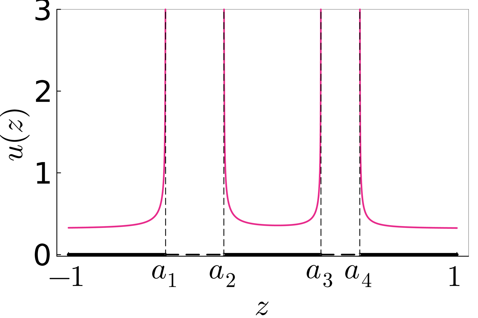
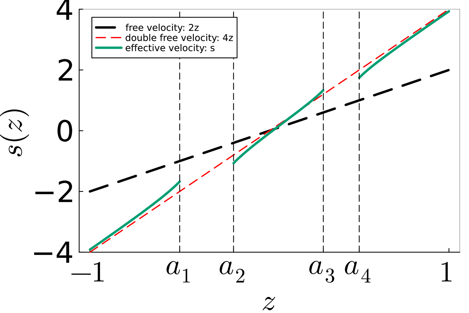
Figure 3: Left: A plot of DOS $u(z)$ whose support is on $[-1,a_{1}]\cup[a_{2},a_{3}]\cup[a_{4},1]$. Right: A plot of effective velocity $s(z)$ which is supported on $[-1,a_{1}]\cup[a_{2},a_{3}]\cup[a_{4},1]$. As shown in the plot, the effective velocity $s(z)$ is approximately equal to twice the free velocity when the gaps become small. Similar velocity doubling phenomenon for fNLS circular condensate was established in [11], [24] and experimentally observed in [8].

Corollary 4.4.

When $a_{4}=a_{3}$, the solution (4.6) and (4.7) reduce to

$$u(z) =u_{0}(z;a_{1},a_{2})=\frac{1}{\pi}\frac{(z-\frac{1}{2}(a_{2}+a_{1}))}{\sqrt{(z-a_{2})(z-a_{1})}},$$ (4.14)

$$v(z) =v_{0}(z;a_{1},a_{2})=\frac{4}{\pi}\frac{(z^{2}-\frac{1}{2}(a_{2}+a_{1})z-\frac{1}{8}(a_{1}-a_{2})^{2})}{\sqrt{(z-a_{2})(z-a_{1})}},$$ (4.15)

where $z\in[-1,a_{1}]\cup[a_{2},1]$, and the radical $\sqrt{(z-a_{1})(z-a_{2})}$ is non-negative on $[a_{2},1]$ and non-positive on $[-1,a_{1}]$. The effective velocity is then given by

$$s(z)=s_{0}(z;a_{1},a_{2})=4z-\frac{\frac{1}{2}(a_{2}-a_{1})^{2}}{z-(a_{2}+a_{1})/2}.$$ (4.16)

Proof.

Using solutions (4.6) and (4.7), taking the limit as $a_{3}\rightarrow a_{4}-$, one obtains (4.14) and (4.15) respectively. ∎

Corollary 4.5.

If in the conditions of Corollary 4.4 we have $a_{1}=a_{2}$, then

$$u_{0}(z)=\frac{1}{\pi},\quad v_{0}(z)=\frac{4z}{\pi}\quad\text{and}\quad s_{0}(z)=4z.$$ (4.17)

We note that the effective velocity in the defNLS condensate with the spectral support $\Gamma=[-1,1]$ is twice the velocity of a free soliton. The same holds true for fNLS circular soliton condensates when the spectral support set $\Gamma^{+}$ in ${\mathbb{C}}^{+}$ is the upper semicircle ([11]).

5 Modulational dynamics for the defNLS soliton gases

If we have a nonhomogeneous defNLS soliton gas the bands evolve with $x,t$ according to

$$u_{t}+v_{x}=0,$$ (5.1)

where $u,v$ are given by (4.3). The following theorem converts (5.1) into a system of PDEs for the end points $a_{j}$ of the bands of $\Gamma$ (branch points for the corresponding Riemann surface $\mathcal{R}$), also known as modulation equations. The proof of this theorem is based on the same arguments as those used in [6], [24] for KdV and fNLS nonhomogeneous soliton condensates respectively. For convenience of the reader, we present this proof below.

Theorem 5.1.

For a nonhomogeneous defNLS soliton condensate with distinct endpoints $a_{j}$, the equation (5.1) is equivalent to the system of modulation equations

$$\partial_{t}a_{j}(x,t)+V_{j}\partial_{x}a_{j}(x,t)=0,\quad j=1,\cdots,2n$$ (5.2)

where

$$\left.V_{j}=\frac{Q(z)}{P(z)}\right|_{z=a_{j}},\qquad j=1,\dots,2n,$$ (5.3)

and the polynomials $P,Q$ are defined in Theorem 4.1.

Proof.

Let us first show that equation (5.1) implies (5.2). Using (4.3), we can write (5.1) as

$$\left(\frac{P}{RR_{0}}\right)_{t}+\left(\frac{Q}{RR_{0}}\right)_{x}=0\qquad\text{or}\qquad\left(\frac{P}{R}\right)_{t}+\left(\frac{Q}{R}\right)_{x}=0,$$ (5.4)

which can be further written as

$$P_{t}+Q_{x}=P(\log(R))_{t}+Q(\log(R))_{x}.$$ (5.5)

Multiplying by $(z-a_{j})$ both sides of (5.5) and taking limit $z\rightarrow a_{j}$, one obtains

$$P(a_{j})(a_{j})_{t}+Q(a_{j})(a_{j})_{x}=0.$$ (5.6)

Note the band vanishing conditions (4.4) imply that zeros of $P$ are located on the bands (one in each). Thus $P(a_{j})\neq 0$. Dividing (5.6) by $P(a_{j})$ one gets equation (5.2), where $V_{j}$ given by (5.3) is bounded.

Assume now the modulation equation for the endpoints $\{a_{j},j=1,\cdots,2n\}$ are given by (5.2). Following the argument in [12] (or the authors’ previous work [24]), we consider the differential

$$\Omega=u_{t}dz+v_{x}dz$$ (5.7)

on the superband RS $\mathcal{R}$, where $u,v$ are given by Theorem 4.1. Then

$$\Omega=\frac{1}{2}\left[\sum_{j=1}^{2N}\frac{P(z)(a_{j})_{t}+Q(z)(a_{j})_{x}}{z-a_{j}}\frac{dz}{R(z)R_{0}(z)}\right]+\frac{P_{t}(z)+Q_{x}(z)}{R(z)R_{0}(z)}dz,$$ (5.8)

which implies that $\Omega$ has at most double poles at $a_{j}$. But the equation (5.2) implies $\Omega$ is holomorphic at $a_{j}$. Note again by Theorem 4.1, we observe that $\Omega$ is holomorphic at $z=\infty$, thus, $\Omega$ is a holomorphic differential on $\mathcal{R}$. Since by (4.4) all the band integrals of $udz$ and $vdz$ are zero, so are their $x,t$ derivatives. We thus get that $\Omega=0$, which implies (5.1).

∎

One can interpret Theorem 5.1 as saying that the kinetic equation for defNLS soliton condensate is equivalent to defNLS-Whitham equations ([17]) for the dynamics of endpoints of spectral bands of slowly modulated finite gap defNLS solutions.

In the rest of the section, we study the time evolution of a nonhomogeneous DOS $u$ of the defNLS soliton condensate of genus zero, which is defined by the initial distribution of $a_{1}(x,t)$ at $t=0$. Without loss of generality, we set $a_{2}=1$ and the branch point $a_{1}$ is the only moving point. According to Theorem 5.1, the dynamics of $a_{1}$ is governed by

$$\partial_{t}a_{1}+V_{1}\partial_{x}a_{1}=0,\quad V_{1}=3a_{1}+1,$$ (5.9)

where the latter expression is obtained by calculating $s_{0}(a_{1};a_{1},1)$ from (4.16). This equation coincides (up to a factor due to the different set-ups for the defocusing NLS equation) with the Whitham equation (2.9) in [17]. It also coincides (up to a factor) with the Whitham equation (1.16a) in [15] for $\hat{\lambda}_{-}$, where $\hat{\lambda}_{+}=1$ is fixed.

The classical Riemann problem consists of finding solution to a system of hyperbolic conservation laws, like (5.2), subject to piecewise-constant initial conditions exhibiting discontinuity, say, at $x=0$. The solution of such Riemann problem generally represents a combination of constant states, simple (rarefaction) waves and strong discontinuities (shocks or contact discontinuities).

Remark 5.2.

The modulation equations (5.2) form a strictly hyperbolic system of first order quasi-linear PDEs provided that all the branch points are distinct (otherwise it will be just hyperbolic). This system is in the diagonal (Riemann) form with all the coefficients (velocities) being real. The Cauchy data for this system consists of $\vec{a}(x,0)$, which denotes the vector of all the endpoints $a_{j}(x,0)$. The system has a unique local (classic) real solution provided $\vec{a}(x,0)$ is of $C^{1}$ class and real and the coefficients $V_{j}(\vec{a})$ are smooth and real (see for example see [9], Theorem 7.8.1).

Remark 5.3.

As it is well known, hyperbolic system may develop singularities in the $x,t$ plane, which, in the case of modulation equations (5.2), lead to collapse of a band or a gap, or to appearance of a new “double point” that will open into a band or gap. In any case, at a point of singularity (also known as a breaking point), two or more endpoints from $\vec{a}(x,t)$ collide or a new pair of collapsed double points appear, so that the Riemann surface $\mathcal{R}$ develop a singularity. This type of situation was observed and discussed in a variety of different settings, see, for example, [22], [3], including in slowly modulated finite gap defNLS solutions [17]. Technically, Theorem 5.1 is not applicable at a breaking point, but, according to general results of [4] (and also [17]), solutions of the modulation equations (5.2) can be continued into regions of different genera beyond breaking points. Some examples of the evolution of the defNLS condensate after the breaking point will be discussed in the rest of the section.

Let us consider the Riemann problem for a genus 0 defNLS condensate determined by the step initial data

$$a_{1}(x,t=0)=\begin{cases}q_{-},&x<0\\ q_{+},&x>0\end{cases},\quad q_{+}\neq q_{-},$$ (5.10)

where $q_{\pm}\in(-1,1)$.

There are two cases depending on whether $q_{-}>q_{+}$ or $q_{-}<q_{+}$. In the first case, it is well known (see [17]) that the equation (5.9) admits a unique global solution (a rarefaction wave). In the second case, higher genus Riemann surfaces are need to describe the evolution of the nonhomogeneous defNLS gas. In this section, we will restrict ourselves to the genus 0 and genus 1 cases. And following similar arguments in [6, 17, 24], we give explicit formulae of DOS/DOF for the nonhomogeneous defNLS gas.

Rarefaction wave: $q_{-}<q_{+}$

In this case, the initial data for $a_{1}$ is given by (5.10) with $q_{-}>q_{+}$. Then the equation (5.9) admits the following rarefaction wave solution:

For $(x,t)\in{\mathbb{R}}\times{\mathbb{R}}_{+}$,

$$a_{1}(x,t)=\begin{cases}q_{-},&x\leq V_{1-}t,\\ -\frac{x}{3t}-\frac{1}{3},&V_{1-}t<x<V_{1+}t,\\ q_{+},&x\geq V_{1+}t,\end{cases}$$ (5.11)

where $V_{1\pm}:=\lim_{a_{1}\rightarrow q_{\pm}}=3q_{\pm}+1$.

Accordingly, the DOS and DOF for the defNLS condensates are given by

$$u(z;x,t)=u_{0}(z;a_{1}(x,t),1)=\frac{1}{\pi}\frac{z-\frac{1+a_{1}(x,t)}{2}}{\sqrt{(z-a_{1}(x,t))(z-1)}},$$ (5.12)

and

$$v(z;x,t)=v_{0}(z;a_{1}(x,t),1)=\frac{4}{\pi}\frac{\left(z^{2}-\frac{1}{2}(1+a_{1}(x,t))z-\frac{1}{8}(a_{1}(x,t)-1)^{2}\right)}{\sqrt{(z-a_{1}(x,t))(z-1)}}.$$ (5.13)

A density plot of the DOS is shown in Fig.4(a), and the dashed line in the plot shows the graph of $a_{1}(x,t)$.

Dispersive shock wave: $q_{-}>q_{+}$

In this case, a wave-breaking occurs immediately, thus we need higher genus DOS to regularize the singularities (see for example in [6] for the KdV condensates). Such regularization is well-known in literature of KdV dispersive shock wave problem. In fact, one can find the following DOS and DOF that regularize the singularities:

$$u(z;x,t) =\begin{cases}u_{0}(z;q_{-},1),&x<V_{2+}t,\\ u_{1}(z;q_{+},a_{2}(x,t),q_{-},1),&V_{2-}t<x<V_{2+}t,\\ u_{0}(z;q_{+},1),&V_{2-}t<x,\end{cases}$$ (5.14)

$$v(z;x,t) =\begin{cases}v_{0}(z;q_{-},1),&x<V_{2+}t,\\ v_{1}(z;q_{+},a_{2}(x,t),q_{-},1),&V_{2-}t<x<V_{2+}t,\\ v_{0}(z;q_{+},1),&V_{2-}t<x,\end{cases}$$ (5.15)

where $a_{2}$ is the only moving branching point, which is governed (similar to (5.9)) by

$$\partial_{t}a_{2}+V_{2}\partial_{x}a_{2}=0,\quad V_{2}=s_{1}(z;q_{+},a_{2},q_{-},1)|_{z=a_{2}},$$ (5.16)

where $s_{1}$ is defined by (4.12). Consider the self-similar reduction, the dynamic of $a_{2}$ is implicitly determined by the following equation:

$$\frac{x}{t}=V_{2}:=(q_{+}+q_{-}+1+a_{2})-\frac{2(a_{2}-q_{+})(a_{2}-q_{-})}{(q_{+}-q_{-})\mu(m)-(a_{2}-q_{-})},$$ (5.17)

where

$$m =\frac{(1-q_{-})(a_{2}-q_{+})}{(q_{-}-q_{+})(1-a_{2})},\quad\mu(m)=\frac{E(m)}{K(m)},.$$ (5.18)

And the critical velocities $V_{2\pm}:=\lim_{a_{2}\rightarrow q_{\pm}}V_{2}$ are explicitly given by

$$V_{2+} =\left(\frac{8q_{+}^{2}-4q_{+}q_{-}-q_{-}^{2}-4q_{+}+2q_{-}-1}{2q_{+}-q_{-}-1}\right),$$ (5.19)

$$V_{2-} =1+2q_{-}+q_{+}.$$ (5.20)

It is easy to check that $V_{2+}<V_{2-}$, which explains why a wave-break occurs immediately. A density plot of the genus one DOS is plot in Fig.4(b), and the dashed line in the plot shows the graph of $a_{2}(x,t)$.

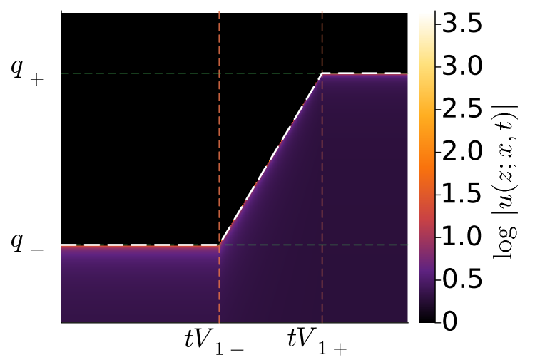
(a)

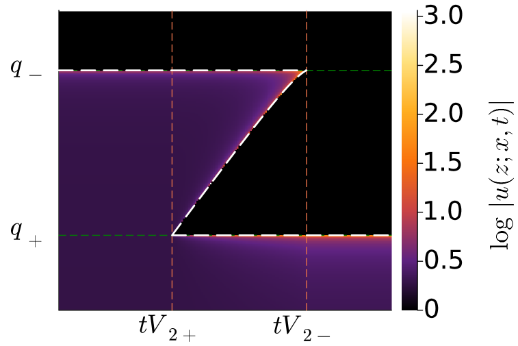
(b)

Figure 4: Solutions to the kinetic equation for the defNLS condensate with step function initial data (Riemann problem) (5.10). (a) Rarefaction wave solution when $q_{-}<q_{+}$; Dashed line: $a_{1}(x,t)$; Colors: the values of DOS $u_{0}(z;a_{1}(x,t),1)$;(b) Dispersive shock wave solution when $q_{-}>q_{+}$. Dashed line: $a_{2}(x,t)$; Colors: the log value of DOS $u_{1}(z;q_{+},a_{2}(x,t),q_{-},1)$.

6 Thermodynamic limit for quasimomentum differentials

The thermodynamic limit of the quasimomentum differential

$$\frac{dp_{N}}{dz}=1-\sum_{j=1}^{\infty}\frac{I_{m,N}}{z^{m+1}}$$ (6.1)

for finite gap solutions for the fNLS defined on $\mathcal{R}_{N}$ was introduced in [23] as

$$\frac{dp}{dz}:=1-\sum_{m=1}^{\infty}\frac{I_{m}}{z^{m+1}},$$ (6.2)

where $I_{m}=\lim_{N\rightarrow\infty}I_{m,N}$, $m\in{\mathbb{N}}$. In the assumption that the length of each band except possibly one does not exceed some $\delta>0$, the coefficients $I_{m,N}$ were shown (Theorem 1.1, [23]) to have the form

$$I_{m,N}=\left[\frac{m}{2\pi i}\sum_{|j|=1}^{N}U_{j,N}\oint_{{\bf B}_{j}}\frac{[\zeta^{m-1}R_{0}(\zeta)]_{+}d\zeta}{R_{0}(\zeta)}+md_{m}\delta_{0}^{m+1}\right](1+O(N^{\frac{1}{2}}\delta)),$$ (6.3)

where: $R_{0}(z)=(z^{2}-\delta_{0}^{2})^{\frac{1}{2}}$ that behaves like $z+o(1)$ as $z\rightarrow\infty$ with $\delta_{0}\in i{\mathbb{R}}^{+}$; the polynomial $[f(\zeta)]_{+}$ consists of the non-negative powers of the Laurent series expansion of $f(\zeta)$ at infinity; $U_{j,N}=\frac{1}{2}k_{j}=\frac{1}{2}\oint_{{\bf A}_{j}}dp_{N}$ with ${\bf A}$-cycles being positively/negatively oriented small loops around each shrinking band in ${\mathbb{C}}^{\pm}$ respectively, and; each ${\bf B}_{j}$ is the ${\bf B}$ cycle on $\mathcal{R}_{N}$ intersecting $[-\delta_{0},\delta_{0}]$ and ${\bf A}_{j}$ and oriented accordingly. Additionally, $d_{m}\delta_{0}^{m+1}$, $m\in{\mathbb{N}}$, denote the coefficient of $z^{-m}$ in the Laurent expansion of $R_{0}(z)$ at infinity, that is, $d_{m}=0$ when $m$ is even and

$$d_{m}=-\frac{1}{m}\frac{m!!}{(m+1)!!}$$ (6.4)

when $m$ is odd.

Based on the expansion (6.2), different expressions for $\frac{dp}{dz}$ in terms of the DOS $u(z)$ were derived for the cases of fNLS soliton and breather gases. In particular, in Theorem 3.18 of [23] it was proven that

$$2g_{x}(z)=i\int_{\Gamma}u(\zeta)\ln\frac{R_{0}(\zeta)R_{0}(z)+\zeta z-\delta_{0}^{2}}{\zeta-z}|d\zeta|+{z-R_{0}(z)},$$ (6.5)

where $z\in\bar{\mathbb{C}}\setminus\Gamma$ and $\frac{dp}{dz}=1-2g_{xz}(z)$.

In view of (3.7), one has

$$2g_{xz}(z)=\frac{i}{R_{0}(z)}\int_{\Gamma}\frac{u(\zeta)R_{0}(\zeta)}{\zeta-z}|d\zeta|+1-\frac{z}{R_{0}(z)},$$ (6.6)

so that

$$\frac{dp}{dz}=\frac{z}{R_{0}(z)}-\frac{i}{R_{0}(z)}\int_{\Gamma}\frac{u(\zeta)R_{0}(\zeta)}{\zeta-z}|d\zeta|=\frac{z}{R_{0}(z)}+\frac{2\pi}{R_{0}(z)}C_{\Gamma}[\breve{u}R_{0}](z),$$ (6.7)

which is the thermodynamic limit of the quasimomentum differential for the breather gas with DOS $u(z)$ on $\Gamma$, where $u(\zeta)|d\zeta|=\breve{u}(\zeta)d\zeta$.

Let us make sure that (6.7) in the limit $\delta\rightarrow 0$ is consistent with the expression for $\frac{dp}{dz}$ for the fNLS soliton gas obtained in Theorem 3.15 [23]. Indeed, using subscripts “bre” and “sol” to distinguish the corresponding quasimomentum differentials and observing $R_{0}(z)\rightarrow z$ as $\delta\rightarrow 0$, in this limit one has

$$\left(\frac{dp}{dz}\right)_{bre}=\frac{z}{R_{0}(z)}+\frac{2\pi}{R_{0}(z)}C_{\Gamma}[\breve{u}R_{0}](z)\rightarrow 1+{2\pi}C_{\Gamma}[\breve{u}](z)=\left(\frac{dp}{dz}\right)_{sol},$$ (6.8)

which follows from

$$\frac{1}{z}\int_{\Gamma}\frac{u(\zeta)\zeta}{\zeta-z}|d\zeta|=\frac{1}{z}\int_{\Gamma}u(\zeta)|d\zeta|+\int_{\Gamma}\frac{u(\zeta)}{\zeta-z}|d\zeta|=\int_{\Gamma}\frac{u(\zeta)}{\zeta-z}|d\zeta|$$ (6.9)

since $u(z)$ is real and anti Schwarz symmetrical.

6.1 Defocusing NLS

Let us go back to defNLS soliton gas. Our current goal is to show that the formula (6.7) for the thermodynamic limit of the quasimomentum differential for fNLS breather gas can be adjusted for the defNLS (dark) soliton gas, where we take $R_{0}(z)=(z^{2}-1)^{\frac{1}{2}}$ and $\Gamma$ to be the accumulation set of the centers of shrinking bands in the thermodynamic limit.

The first step is to verify that the expression (6.3) is valid for the quasimomentum differential $dp_{N}$ for the Riemann surface $\mathcal{R}_{N}$ for defNLS finite gap solutions, which was introduced in (2.3). Expression (6.3) for fNLS was derived by considering the $g$-function for finite gap solutions on $\mathcal{R}_{N}$. This procedure is similar for defNLS ([29]), where the Riemann surface $\mathcal{R}_{N}$ has $N+1$ branchcuts $\gamma_{j,N}\subset[-1,1]$. The g-function $g_{x}$ is defined by the RHP

$$g_{x+}(z)+g_{x-}(z)=z+W_{j},\quad z\in\gamma_{j,N},$$ (6.10)

where $g_{x}(z)$ must be analytic in $\bar{\mathbb{C}}\setminus\cup_{j=1}^{N+1}\gamma_{j,N}$, $W_{N+1}=0$ and the real constants $W_{j}$, $j=1,\dots,N$ are to be determined by the requirement that $g_{x}$ is analytic at $z=\infty$. Then, by Sokhotski-Plemelj formula,

$$2g_{x}(z)=\frac{\tilde{R}(z)}{2\pi i}\sum_{j=1}^{N+1}\oint_{\gamma_{j,N}}{\frac{[\zeta+W_{j}]d\zeta}{(\zeta-z)\tilde{R}(\zeta)}}=$$ (6.11)

$${\frac{\tilde{R}(z)}{2\pi i}}\left[\sum_{j=1}^{N+1}\oint_{\gamma_{j,N}}{\frac{\zeta d\zeta}{(\zeta-z)\tilde{R}(\zeta)}}+\sum_{j=1}^{N+1}U_{j,N}\oint_{{\bf B}_{j}}\frac{d\zeta}{(\zeta-z)\tilde{R}(\zeta)}\right],$$ (6.12)

where $\tilde{R}(z)=R_{0}(z)R(z)$, see (2.4), $z$ is outside of each loop and, as in [11], $U_{j,N}:=W_{j+1}-W_{j}=\frac{1}{2}k_{j}$ (see (1.2) and the definition of ${\bf A}$ cycles below equation (2.5)). Equation (6.11) has the same form as the expression for the g-function for the fNLS in [23], and the thermodynamic limit of integrals over $\bf B$ cycles and the scaling in both situations are the same. Therefore, expressions (6.3) for the defNLS soliton gases reads:

$$I_{m,N}=\left[\frac{m}{2\pi i}\sum_{j=1}^{N}U_{j,N}\oint_{{\bf B}_{j}}\frac{[\zeta^{m-1}R_{0}(\zeta)]_{+}d\zeta}{R_{0}(\zeta)}+md_{m}\delta_{0}^{m+1}\right](1+O(N^{\frac{1}{2}}\delta)).$$ (6.13)

Repeating the arguments of Theorem 3.18 from [23] with the limiting spectral support $\Gamma=\cup_{j=1}^{n}c_{j,n}$ to show that (6.7) coincides with $\frac{dp}{dz}$ for the defNLS soliton gas, defined by (6.2).

Proposition 6.1.

The thermodynamic limit $\frac{dp}{dz}$ of quasimomentum differentials $\frac{dp_{N}}{dz}$ from (2.3) is given by (6.7) with $\Gamma=\cup_{j=1}^{n}c_{j,n}$ and $R_{0}=(z^{2}-1)^{\frac{1}{2}}\sim z$ as $z\rightarrow\infty$.

Let us apply Proposition 6.1 to the genus 0 condensate with $\Gamma=[-1,1]$. According to (4.17) $u(z)=\frac{1}{\pi}$. Substituting that into (6.7) with $R_{0}(z)=\sqrt{z^{2}-1}$ and using

$$\int_{-1}^{1}\frac{u(\zeta)R_{0}(\zeta)d\zeta}{\zeta-z}=\frac{1}{2\pi}\oint\frac{R_{0}(\zeta)d\zeta}{\zeta-z}=i(R_{0}(z)-z),$$ (6.14)

we obtain

$$\frac{dp}{dz}=1.$$ (6.15)

That means that $\langle|\psi|^{2}\rangle$, as well as the higher average conserved densities for realizations of such condensate are zeroes, see Section 7 below, i.e., the genus zero defNLS soliton condensate with spectral support $\Gamma$ coinciding with the background is vacuous.

Let us summarize some results from [23] about the thermodynamic limit $\frac{dp}{dz}=\lim_{N\rightarrow\infty}\frac{dp_{N}}{dz}$, see Section 1, of the quasimomentum differential $dp_{N}$ for fNLS soliton and breather gases.

Remark 6.2.

It is interesting to calculate $\frac{dp}{dz},\frac{dq}{dz}$ for the fNLS Akhmediev breather condensate with $\gamma_{0}=[-i,i]$ and $\Gamma$ coinciding with the left shore of $\gamma_{0}$ oriented up. It easily follows from (1.9) that $u(z)\equiv 0$ (in fact, true for any $\Gamma^{+}\subset[0,i]$). The second NDR (1.10) after some calculations yields $v(z)=\frac{4z}{i\pi}$. Substituting $u,v$ into (6.7), (6.17), one obtains

$$\frac{dp}{dz}=\frac{z}{R_{0}(z)}=1+\frac{1}{2z^{2}}+\frac{3}{8z^{4}}+\dots,\qquad\frac{dq}{dz}=2R_{0}(z)-\frac{2z^{2}+2}{R_{0}(z)}+4z=4z.$$ (6.16)

In light of the Section 7 below, we calculate that for this fNLS breather gas the kurtosis $\kappa=2$.

Proposition 6.3.

The thermodynamic limit $dq/dz$ of the quasienergy differential $dq_{N}/dz$ is given by

$$\frac{dq}{dz} =2R_{0}(z)+\frac{2z^{2}}{R_{0}(z)}-\frac{i}{R_{0}(z)}\int_{\Gamma}\frac{v(\zeta)R_{0}(\zeta)d\zeta}{\zeta-z},$$ (6.17)

where $\Gamma=\cup_{j=1}^{n}c_{j,n}$ and $R_{0}=\sqrt{z^{2}-1}\sim z$ as $z\rightarrow\infty.$

Proof.

To derive the thermodynamic limit for the quasienergy differentials, we need to modify the $g$-function set-up accordingly. In fact, similarly to (6.10), we have

$$g_{t+}(z)+g_{t-}(z)=2z^{2}+\tilde{W_{j}},\quad z\in\gamma_{j,N},$$ (6.18)

where all other requirements are exactly the same as for deriving the thermodynamic limit of quasimomentum and the constants $\tilde{W}_{j}$ are determined by the requirement that $g_{t}$ is analytic at $z=\infty$. Repeating the same argument of Theorem 3.18 in [23], taking the thermodynamic limit, we obtain

$$\frac{2g_{t}}{R_{0}}=\sum_{m=0}\frac{H_{m}}{z^{m+1}},$$ (6.19)

where

$$H_{m}=-\int_{\Gamma}v(\xi)\int_{\xi}^{1}\frac{\mu^{m}d\mu}{R_{0}(\mu)}d\xi-\frac{1}{2\pi i}\oint_{A_{0}}\frac{2\xi^{m+2}d\xi}{R_{0}(\xi)},$$ (6.20)

$\Gamma=\sum_{j=1}^{n}c_{j,n}$ is the spectral support and $A_{0}$ is negative oriented large circle enclosing interval $[-1,1]$. Thus, we have

$$\frac{2g_{t}}{R_{0}} =-\frac{i}{R_{0}(z)}\int_{\Gamma}v(\xi)\log\frac{R_{0}(\xi)R_{0}(z)+z\xi-\delta_{0}^{2}}{\xi-z}d\xi+\frac{1}{2\pi i}\oint_{A_{0}}\frac{2\xi^{2}}{(\xi-z)R_{0}(\xi)}d\xi$$ (6.21)

$$=-\frac{i}{R_{0}(z)}\int_{\Gamma}v(\xi)\log\frac{R_{0}(\xi)R_{0}(z)+z\xi-\delta_{0}^{2}}{\xi-z}d\xi+\frac{2z^{2}}{R_{0}(z)}-2z,$$ (6.22)

where the last two terms come from the residue theorem. It follows that

$$2g_{tz}=-\frac{i}{R_{0}(z)}\int_{\Gamma}\frac{v(\xi)R_{0}(\xi)|d\xi|}{\xi-z}+4z-2R_{0}(z)-\frac{2z^{2}}{R_{0}(z)}.$$ (6.23)

Since $dq/dz=4z-2g_{tz}$, we have

$$\frac{dq}{dz}=\frac{dq}{dz} =2R_{0}(z)+\frac{2z^{2}}{R_{0}(z)}+\frac{i}{R_{0}(z)}\int_{\Gamma}\frac{v(\zeta)R_{0}(\zeta)d\zeta}{\zeta-z}.$$ (6.24)

∎

Let us now consider $\frac{dp}{dz}$ and $\frac{dq}{dz}$ for defNLS soliton condensates described in Theorem 4.1, where $u,v$ are proportional to the densities of the quasimomentum and quasienergy meromorphic differentials on the Riemann surface $\mathcal{R}$. In particular, according to Remark (4.2), $u(z)=\frac{idp_{\infty}}{\pi dz}$. Substitute $u(z)$, see (4.3), into (6.7). Then (6.7) becomes

$$-\frac{i}{R_{0}(z)}\int_{\Gamma}\frac{u(\zeta)R_{0}(\zeta)}{\zeta-z}|d\zeta|=\frac{1}{2\pi iR_{0}(z)}\oint_{C}\frac{\pi P(\zeta)d\zeta}{R(\zeta)(\zeta-z)}=\frac{dp_{\infty}}{dz}(z)-\frac{z}{R_{0}(z)},$$ (6.25)

where $C$ is a negatively oriented contour containing $\Gamma$ but not containing $z$. Equation (6.25) together with (6.7) implies

$$\frac{dp_{\infty}}{dz}=\frac{dp}{dz}.$$ (6.26)

Thus, we obtain the following theorem.

Theorem 6.4.

The quasimomentum differential $\frac{dp_{\infty}}{dz}$ on the “superband” Riemann surface $\mathcal{R}$, see (6.26), coincides with $\frac{dp}{dz}$, given by (6.7). Similar statement is true for the quasienergy differentials.

Corollary 6.5.

All the corresponding average densities and fluxes of defNLS soliton condensates with the spectral support $\Gamma$ and of defNLS finite gap solutions on $\mathcal{R}$ defined by $\Gamma$ (see Remark 4.2) coincide.

7 Kurtosis for the genus 0 and genus 1 defNLS gas

In this section, we compute the kurtosis $\kappa$ for the defNLS gas, which is defined by

$$\kappa=\frac{\braket{|\psi|{}^{4}}}{\braket{|\psi|{}^{2}}^{2}},$$ (7.1)

where $\psi$ is a defNLS soliton gas realization and the bracket stands for the ensemble average. It is well known ([12], [13]) that the averaged conserved quantities (densities and fluxes) for the multiphase (finite gap) solution to the integrable PDEs can be computed by expanding the quasimomentum and quasienergy meromorphic differentials on the underlying Riemann surface. The corresponding computations for the averaged conserved quantities of the fNLS soliton/breather gases are derived by the authors in [23]. In fact, based on Proposition 6.1 and 6.3, we can compute the averaged conserved quantities (densities and fluxes) of the defNLS gases by computing the coefficients of (6.7) and (6.17) respectively, where $\Gamma$ is the spectral support.

Corollary 7.1.

The thermodynamic limits $dp/dz$ and $dq/dz$ of the densities of the quasimomentum and quasienergy differentials respectively admit the following expansions as $z\rightarrow\infty$:

$$\frac{dp}{dz} =1-\sum_{m=1}^{\infty}\frac{I_{m}}{z^{m+1}},$$ (7.2)

$$\frac{dq}{dz} =1-\sum_{m=1}^{\infty}\frac{J_{m}}{z^{m+1}},$$ (7.3)

where

$$I_{m} =\int_{\Gamma}u(\zeta)\left[\frac{\zeta^{m}}{R_{0}(\zeta)}\right]_{+}\sqrt{1-\zeta^{2}}d\zeta+md_{m},$$ (7.4)

$$J_{m} =\int_{\Gamma}v(\zeta)\left[\frac{\zeta^{m}}{R_{0}(\zeta)}\right]_{+}\sqrt{1-\zeta^{2}}d\zeta+2md_{m+1},$$ (7.5)

and $d_{m}$ is given by equation (6.4).

Proof.

According Proposition 6.1, the thermodynamic limit of the defNLS quasimomentum differential $\frac{dp_{N}}{dz}$ is given by equation (6.7). Next, we expand (6.7) at $z=\infty$. Recall that

$$R_{0}(z)=\sum_{k=-1}^{\infty}d_{k}z^{-k},$$

where $d_{k}$ is given by (6.4) and $d_{-1}=1$. We also introduce $\tilde{d}_{k}$ so the reciprocal of $R_{0}(z)$ admits the following expansion at $\infty$: $1/R_{0}(z)=\sum_{k=1}^{\infty}\tilde{d}_{k}z^{-k}$. Since $R^{\prime}_{0}(z)=z/R_{0}(z)$, we have $\tilde{d}_{k}=(2-k)d_{k-2},k\geq 1$. Moreover, the coefficient of $z^{-(m+1)}$ of $z/R_{0}(z)$ is $md_{m}$.

Expanding the integral term in (6.7) we have

$$-\frac{i}{R_{0}(z)}\int_{\Gamma}\frac{u(\zeta)R_{0}(\zeta)}{\zeta-z}d\zeta =i\int_{\Gamma}u(\xi)\left(\sum_{k=1}^{\infty}\tilde{d}_{k}z^{-k}\right)R_{0}(\zeta)\sum_{k=0}^{\infty}\zeta^{k}z^{-(k+1)}d\zeta$$

$$=\sum_{m=1}^{\infty}z^{-(m+1)}\int_{\Gamma}iu(\zeta)\left(\sum_{k=1}^{m}\tilde{d}_{k}\zeta^{m-k}\right)R_{0}(\zeta)d\zeta$$

$$=-\sum_{m=1}^{\infty}z^{-(m+1)}\int_{\Gamma}u(\zeta)\left[\frac{\zeta^{m}}{R_{0}(\zeta)}\right]_{+}\sqrt{1-\zeta^{2}}d\zeta$$

Extracting the coefficient of $z^{-(m+1)}$, we then get

$$I_{m}=\int_{\Gamma}u(\zeta)\left[\frac{\zeta^{m}}{R_{0}(\zeta)}\right]_{+}\sqrt{1-\zeta^{2}}d\zeta+md_{m}.$$ (7.6)

Similarly, one can get the coefficients for the quasienergy differential $\frac{dq}{dz}$ by expanding (6.17). In fact, we have

$$2R_{0}(z)+2z^{2}/R_{0}(z)=2R_{0}(z)+2zR_{0}(z)=\sum_{k=-1}^{\infty}(2d_{k}-2kd_{k})z^{-k}.$$

Thus, the coefficient of $z^{-(m+1)}$ is $-2md_{m+1}$. The coefficients extracting from the integral term of (6.17) can be obtained similarly as for (7.4) by replacing $u$ with $v$. ∎

Next, we compute the averaged densities and fluxes for the defNLS gases. The densities and fluxes for the defNLS equation can be derived using so-called quadratic eigenfunction method (see [13]). To compute the kurtosis, it suffices to use just the first few densities and fluxes. They are

$$f_{1} =|\psi|^{2},$$ (7.7)

$$f_{3} =|\psi|^{4}+|\psi_{x}|^{2},$$ (7.8)

$$g_{2} =|\psi|^{4}+2|\psi_{x}|^{2}.$$ (7.9)

Based on Corollary 6.4 and the same normalization as for the fNLS circular gas in [24], we get the following formulae for computing the averaged densities and fluxes for the defNLS gas:

$$I_{1} =-\frac{1}{2}\braket{f_{1}}:=-\frac{1}{2}\braket{|\psi|{}^{2}},$$ (7.10)

$$I_{3} =-\frac{3}{8}\braket{f_{3}}:=-\frac{3}{8}\braket{|\psi|{}^{4}+|\psi_{x}|^{2}},$$ (7.11)

$$J_{2} =-\frac{1}{2}\braket{g_{2}}:=-\frac{1}{2}\braket{|\psi|{}^{4}+2|\psi_{x}|^{2}}.$$ (7.12)

Applying Corollary 7.1 we obtain

$$I_{1} =-1/2+\int_{\Gamma}u(\zeta)\sqrt{1-\zeta^{2}}d\zeta,$$ (7.13)

$$I_{3} =-3/8+\int_{\Gamma}(\zeta^{2}+1/2)u(\zeta)\sqrt{1-\zeta^{2}}d\zeta,$$ (7.14)

$$J_{2} =-1/2+\int_{\Gamma}\zeta v(\zeta)\sqrt{1-\zeta^{2}}d\zeta,$$ (7.15)

where $u,v$ are the DOS and DOF for the defNLS gas, given by Theorem 4.1. Using equations (7.10) ,(7.11) and (7.12) one obtains

$$\braket{|\psi|{}^{2}}=2I_{1}=1-2\int_{\Gamma}u(\zeta)\sqrt{1-\zeta^{2}}d\zeta,$$ (7.16)

and

$$\braket{|\psi|{}^{4}} =-\frac{16}{3}I_{3}+2J_{2}$$

$$=1-\frac{16}{3}\int_{\Gamma}\left(\zeta^{2}+\frac{1}{2}\right)u(\zeta)\sqrt{1-\zeta^{2}}d\zeta+2\int_{\Gamma}\zeta v(\zeta)\sqrt{1-\zeta^{2}}d\zeta.$$ (7.17)

By the definition of kurtosis (7.1), we have the following formula for computing the kurtosis of the defNLS condensate:

$$\kappa =\frac{\frac{1}{2}J_{2}-\frac{4}{3}I_{3}}{I_{1}^{2}}$$

$$=\frac{1-\frac{16}{3}\int_{\Gamma}\left(\zeta^{2}+\frac{1}{2}\right)u(\zeta)\sqrt{1-\zeta^{2}}d\zeta+2\int_{\Gamma}\zeta v(\zeta)\sqrt{1-\zeta^{2}}d\zeta}{(1-2\int_{\Gamma}u(\zeta)\sqrt{1-\zeta^{2}}d\zeta)^{2}}.$$ (7.18)

We summarize the above computation as the following lemma.

Lemma 7.2.

For any defNLS condensate with spectral support $\Gamma$, the kurtosis can be computed by the formula (7), which admits another representation:

$$\kappa=\frac{1-\int_{\Gamma}\left(\frac{16}{3}(\zeta^{2}+\frac{1}{2})P(\zeta)-2\zeta Q(\zeta)\right)\frac{d\zeta}{R(\zeta)}}{\left(1+\int_{\Gamma}2P(\zeta)\frac{d\zeta}{R(\zeta)}\right)^{2}},$$ (7.19)

where polynomials $P,Q$ are given in Theorem 4.1.

Proof.

Using the DOS($u$)/DOF($v$) representations (see equation (4.3)) as given in Theorem4.1, plugging in formula (7), and after simplification, we obtain the kurtosis formula as stated. ∎

Remark 7.3.

The averaged conserved quantity (see equation (7.13)) was also previously presented in [5], see equation (28) there. In fact, following the argument in [5] (section III), one can derive the formulae (7.14) and (7.15) as well. The idea is to use the dark soliton solution (see [28]) of the defNLS equation, which is given by

$$\psi(x,t;z)=\frac{(z+i\sqrt{1-z^{2}})^{2}+A}{1+A}{e^{-2it}},\quad A=e^{2\sqrt{1-z^{2}}(x-2zt)}.$$ (7.20)

One can rewrite the solution in the form of

$$\psi(x,t;z)=\sqrt{\rho}e^{iS(x,t)},$$

where

$$\rho(x,t) :=|\psi(x,t;z)|^{2}=1-(1-z^{2})\hbox{sech}^{2}(\sqrt{1-z^{2}}(x-2zt)),$$ (7.21)

$$S(x,t) :=\text{Arg}(\psi)=\arctan\frac{2z\sqrt{1-z^{2}}}{A-1+2z^{2}},$$ (7.22)

which coincide (up to a factor $2$ in the linear dispersion relation, due to the different settings for the defocusing NLS equation) with equation (10) in [5], where $u_{s}^{\pm}$ in [5] is just the $x$-derivative of the phase, $\partial_{x}S$. Then, following [5], we can compute the ensemble average of the densities and fluxes for the defNLS soliton gas as follows:

$$I_{3} =-\frac{3}{8}\braket{f_{3}[\psi(x,t;z)]}$$ (7.23)

$$=-\frac{3}{8}\left(\int_{\Gamma}u(z)\left(\int_{\mathbb{R}}(f_{3}[\psi(x,t;z)]-1)dx\right)dz+1\right)$$ (7.24)

$$=-\frac{3}{8}\left(\int_{\Gamma}u(z)\left(\int_{\mathbb{R}}(f_{3}[\psi(x,0;z)]-1)dx\right)dz+1\right).$$ (7.25)

The last step follows from the fact integral of $\int_{\mathbb{R}}(f_{3}-1)dx$ is invariant in $t$. A direct computation of the last integral gives (7.14). Similarly, one can get equation (7.15) by computing the following integral:

$$J_{2}=-\frac{1}{2}\left(\int_{\Gamma}v(z)\left(\int_{{\mathbb{R}}}(g_{2}[\psi(0,t;z)]-1)dt\right)dz+1\right)$$ (7.26)

7.1 Kurtosis for genus 1 and 0 defNLS condensates

In this subsection, we restrict the discussion to the genus one and genus zero condensate cases, where the explicit expressions for $u,v$ were calculated in Section 4. The theorem below gives the kurtosis formula for general genus one defNLS condensate.

Theorem 7.4.

For a general genus one defNLS condensate(i.e for each $\{a_{j}\}_{j=1}^{4}$ such that $-1\leq a_{1}<a_{2}<a_{3}<a_{4}\leq 1$), the corresponding kurtosis is given by the following expression:

$$\kappa=\frac{A\mu+B}{3(C\mu+D)^{2}},$$ (7.27)

where

$$A =-8\left(-a_{4}+a_{2}\right)\left(-a_{3}+a_{1}\right)\left(4\sum_{j=1}^{4}a_{j}^{2}-(\sum_{j=1}^{4}a_{j})^{2}\right),$$

$$B =3a_{1}^{4}+\left(12a_{2}-12a_{3}-12a_{4}\right)a_{1}^{3}$$

$$+(2a_{2}^{2}+\left(-20a_{3}-20a_{4}\right)a_{2}+18a_{3}^{2}+20a_{4}a_{3}+18a_{4}^{2})a_{1}^{2}$$

$$+(12a_{2}^{3}-4(a_{3}+a_{4})(5a_{2}^{2}-5a_{3}a_{2}-5a_{4}a_{2}+3a_{3}^{2}+2a_{4}a_{3}+3a_{4}^{2}))a_{1}$$

$$+3a_{2}^{4}+\left(-12a_{3}-12a_{4}\right)a_{2}^{3}+\left(18a_{3}^{2}+20a_{4}a_{3}+18a_{4}^{2}\right)a_{2}^{2}$$

$$+\left(-12a_{3}^{3}-20a_{3}^{2}a_{4}-20a_{3}a_{4}^{2}-12a_{4}^{3}\right)a_{2}$$

$$+3a_{3}^{4}+12a_{3}^{3}a_{4}+2a_{3}^{2}a_{4}^{2}+12a_{3}a_{4}^{3}+3a_{4}^{4}$$

$$C =4\left(-a_{4}+a_{2}\right)\left(-a_{3}+a_{1}\right),\qquad D=-(a_{1}+a_{2}-a_{3}-a_{4})^{2},$$

$$\mu =\frac{E(m)}{K(m)},\qquad m=\frac{\left(a_{3}-a_{4}\right)\left(-a_{2}+a_{1}\right)}{\left(a_{2}-a_{4}\right)\left(-a_{3}+a_{1}\right)}.$$

Proof.

Plugin the genus one DOS/DOF, which are given in Theorem 4.1, into the kurtosis formula (7), direct computation gives the result. ∎

Corollary 7.5.

For a general genus zero defNLS condensate the kurtosis is always 1.

Proof.

Using the DOS/DOF of the genus zero condensate (see Corollary 4.4), by the residue computations, we have

$$\braket{|\psi|{}^{2}}=\frac{(a_{1}-a_{2})^{2}}{4},$$ (7.28)

$$\braket{|\psi|{}^{4}}=\frac{(a_{1}-a_{2})^{4}}{16}.$$ (7.29)

Then it follows that the kurtosis is 1 for any $-1<a_{1}<a_{2}<1$. ∎

Remark 7.6.

Using (7.11) and equation (7.29), we obtain, for genus zero condensate, we have

$$\braket{|\psi_{x}|{}^{2}}=\frac{(a_{1}^{2}-a_{2}^{2})^{2}}{4}.$$ (7.30)

Remark 7.7.

In the vacuum case, the support of the realization of the dark soliton fill the whole interval $[-1,1]$ and we have $u=1/\pi$ and $v=4z/\pi$. By taking the limit $a_{1}\rightarrow a_{2}$ in (7.28) and (7.29), we obtain that

$$\braket{|\psi|{}^{4}}=0,\quad\braket{|\psi|{}^{2}}=0.$$ (7.31)

Corollary 7.5 shows that, similarly to KdV soliton condensates ([6]), the genus zero soliton condensate is almost surely given by a constant amplitude solution to the defNLS since the variance $\sqrt{\braket{|\psi|{}^{4}}-\braket{|\psi|{}^{2}}^{2}}=0$. Moreover, in the case $a_{1}=-a_{2}$, it follows from (7.30) that the phase $\arg\psi$ is almost surely a constant. We now analyze the general case $a_{1}\neq-a_{2}$.

The Madelung transformation reduces the NLS (1.1) to the hydrodynamic type system

$$\frac{1}{2}\rho_{t}+(\rho\mu)_{x}=0,\qquad\frac{1}{2}(\rho\mu)_{t}+(\rho\mu^{2}-s\frac{1}{2}\rho^{2})_{x}=\frac{1}{4}[\rho(\ln\rho)_{xx}]_{x},$$ (7.32)

where $\rho=|\psi|^{2}$, $\mu=(\arg\Psi)_{x}$ and $s=-1$ for defNLS. If $\psi$ is a generic realization of defNLS genus zero soliton condensate then $\rho_{t}=0$ and from the first (7.32) equation we obtain $\arg\psi=k(t)x+c(t)$ for some functions $k(t),c(t)$ to be determined. Substituting $\mu=k(t)$ into the second (7.32) equation we see that $k$ is independent of $t$. Thus,

$$\psi(x,t)=\frac{b-a}{2}e^{i(kx+c(t))}.$$ (7.33)

Now, using (7.30), we find $k=(b+a)$. Substituting (7.33) to (1.1), we find $c(t)=\omega t$ with some constant $\omega$. Thus, the realization we consider almost surely has the form

$$\psi(x,t)=\frac{1}{2}(b-a)e^{i[(b+a)x+\omega t]},$$ (7.34)

which is also the form of a plane wave solution defined by a spectral band $[a,b]$ (up to a constant phase). Thus, we extended the observation of [6] that a genus zero KdV condensate almost surely coincides with the corresponding genus zero KdV solution for defNLS genus zero condensates.

According to Theorem 6.4 and its Corollary 6.4, the averaged conserved quantities for the genus one defNLS condensate coincides with the averaged conserved quantities for a genus one finite gap solution of the defNLS equation constructed from the same Riemann surface. Thus, to compute the kurtosis for the defNLS condensate is equivalent to compute the kurtosis for a genus one finite gap solution of the defNLS equation. In fact, to compute the kurtosis, we only need to know the modulus of the genus one solution to the defNLS equation. Given the same Riemann surface as for the defNLS condensate, it is well known(see [16], chapter 5, Section 2) that

$$|\psi(x,t)|^{2}=\frac{1}{4}(a_{1}-a_{2}-a_{3}+a_{4})^{2}+(a_{2}-a_{1})(a_{4}-a_{3})\text{sn}^{2}\left(\Lambda(x,t),m\right),$$ (7.35)

where $\Lambda(x,t)=\sqrt{(a_{4}-a_{2})(a_{3}-a_{1})}\left(x-t\sum_{j=1}^{4}a_{j}\right),$ where $m=\frac{\left(a_{3}-a_{4}\right)\left(-a_{2}+a_{1}\right)}{\left(a_{2}-a_{4}\right)\left(-a_{3}+a_{1}\right)}$ is given by (7.27). Then by definition of the kurtosis we get :

$$\kappa=\frac{\frac{1}{T}\int_{0}^{T}|\psi(x,t)|^{4}dx}{\left(\frac{1}{T}\int_{0}^{T}|\psi(x,t)|^{2}dx\right)^{2}}=\frac{T\int_{0}^{T}|\psi(x,0)|^{4}dx}{\left(\int_{0}^{T}|\psi(x,0)|^{2}dx\right)^{2}},$$ (7.36)

where $T=2K(m)/\sqrt{(a_{4}-a_{2})(a_{3}-a_{1})}$ is the period of $|\psi(x,0)|$. Note that the second equality follows from the fact that varying $t$ only shifts the genus-one finite-gap solution but without changing its spatial average. Using the new representation, we can show that the kurtosis for the genus one condensate is always bounded by 3/2 from above and bounded (trivially) by 1 from below.

Theorem 7.8.

For general genus one defNLS condensate, the kurtosis satisfies the following inequality:

$$1\leq\kappa\leq 3/2.$$

Proof.

The lower bound is a consequence of Cauchy-Schwartz inequality. Next we prove the upper bound.

Based on the new representation ((7.36)) of the kurtosis in terms of integrals of Jacobi theta functions, it is convenient to introduce some new notations:

$$b=\frac{1}{4}(a_{1}-a_{2}-a_{3}+a_{4})^{2},\quad A=(a_{2}-a_{1})(a_{4}-a_{3}).$$ (7.37)

Then equation (7.36) becomes

$$\kappa=\frac{T\int_{0}^{T}\left[b+A\,\text{sn}^{2}(\Lambda(x,0),m)\right]^{2}dx}{\left(\int_{0}^{T}[b+A\,\text{sn}^{2}(\Lambda(x,0),m)]dx\right)^{2}},$$ (7.38)

where using the new notation, $\Lambda(x,0)=\sqrt{A/m}x$. First, assuming $A,b$ and $m$ are independent variables and fixing $m,A$, we find after simple calculations

$$\partial_{b}\kappa =2T\frac{\left(\int_{0}^{T}\left(A\,\text{sn}^{2}(\Lambda(x,0),m)+b\right)dx\right)^{2}-T\int_{0}^{T}\left(A\text{sn}^{2}(\Lambda(x,0),m)+b\right)^{2}dx}{\left(\int_{0}^{T}\left((A\text{sn}^{2}(\Lambda(x,0),m)+b\right)dx)\right)^{3}}\leq 0.$$

where with used that, according to the Cauchy-Schwartz inequality,

$$\left(\int_{0}^{T}\left(A\,\text{sn}^{2}(\Lambda(x,0),m)+b\right)dx\right)^{2}\leq T\left(\int_{0}^{T}\left(A\,\text{sn}^{2}(\Lambda(x,0),m)+b\right)^{2}dx\right).$$

Thus, we have $\kappa\leq\kappa|_{b=0}.$ When $b=0$, the kurtosis becomes

$$\kappa(m):=\kappa|_{b=0} =\frac{T\int_{0}^{T}\text{sn}^{4}(\sqrt{A/m}x,m)dx}{(\int_{0}^{T}\text{sn}^{2}(\sqrt{A/m}x,m)dx)^{2}}=\frac{2K(m)\int_{0}^{2K(m)}\text{sn}^{4}(y,m)dy}{(\int_{0}^{2K(m)}\text{sn}^{2}(y,m)dy)^{2}}.$$

Using formulae (310.02) and (310.04) in [1], the expression for the kurtosis can be further simplified to

$$\kappa(m)=\frac{2+m-2(1+m)\mu}{3(\mu-1)^{2}},$$ (7.39)

where $\mu$ is given in (7.27).

To show $\kappa(m)\leq 3/2$, it is sufficient to show

$$F(\mu)=9\mu^{2}+2(2m-7)\mu+5-2m\geq 0,\forall m\in[0,1].$$ (7.40)

The discriminant of $F(\mu)$ (regard $\mu$ as independent variable) is given by $8(2m-1)(m-2)$. Since $m\leq 1$, the discriminant of $F$ is negative for $m>1/2$. And since the leading coefficient of $F$ is positive, we then have shown that for $m\geq 1/2$, $F\geq 0$, which in turn implies $\kappa(m)\leq 3/2$ for $m\geq 1/2$.

Next, we show that $\kappa(m)\leq 3/2$ for $m\in[0,1/2]$. Using Theorem A.1, we have

$$\mu(m):=\frac{E}{K}\geq 1-m/2-m^{2}/16-\frac{7}{100}m^{3}.$$ (7.41)

To prove that $F(\mu)>0$,it is sufficient to show the lower bound (7.41) is larger than the largest root of $F$, which is $\frac{1}{9}(7-2m+\sqrt{2(2m-1)(m-2)})$. Since

$$\left[9(1-m/2-m^{2}/16-\frac{7}{100}m^{3})-(7-2m)\right]^{2}-2(2m-1)(m-2)$$

$$=2(1-2m)+\frac{117}{400}m^{3}+\frac{4437}{1280}m^{4}+\frac{567}{800}m^{5}+\frac{3969}{10000}m^{6}>0,\,\,\forall m\in[0,1/2],$$

we have

$$\mu(m)\geq 1-m/2-m^{2}/16-\frac{7}{100}m^{3}>\frac{1}{9}(7-2m+\sqrt{2(2m-1)(m-2)}),$$

which then implies $F(\mu)>0$ whenever $m\in[0,1/2]$.

Thus, for all $m\in[0,1]$, we have $F\geq 0$, which in turn implies $\kappa(m)\leq 3/2$ for any $m\in[0,1]$. ∎

8 Diluted defNLS condensate

Consider now the diluted genus 0 defNLS condensate with $u(z)=\frac{\alpha}{\pi}$, where $\alpha\in(0,1)$. It follows then from (2.12) that

$${\sigma}(z)=\frac{\pi(1-\alpha)}{\alpha}|R_{0}(z)|.$$ (8.1)

We use (6.7) and (6.14) to calculate

$$\frac{dp}{dz}=\alpha+(1-\alpha)\frac{z}{R_{0}(z)}=1+(1-\alpha)\left(\frac{1}{2z^{2}}+\frac{3}{8z^{4}}+\dots\right),$$ (8.2)

which expresses the average conserved densities through the binomial coefficients of the expansion of $\frac{1}{\sqrt{1-z^{-2}}}$ at $z=\infty$. In particular,

$$I_{1}=\frac{\alpha-1}{2},\qquad I_{3}=\frac{3(\alpha-1)}{8},$$ (8.3)

etc., where

$$\frac{dp}{dz}=1-\sum_{m=1}^{\infty}\frac{I_{m}}{z^{m+1}}.$$ (8.4)

Given that $\langle|\psi|^{2}\rangle=-2I_{1}$ , we obtain

$$\langle|\psi|^{2}\rangle=1-\alpha,$$ (8.5)

i.e., we have the vacuum $\langle|\psi|^{2}\rangle=0$ in the case of the condensate $\alpha=1$.

We are now trying to solve the 2nd NDR (3.11) with ${\sigma}$ given by (8.1) by $v(z)=bz$. Then

$$\sqrt{1-z^{2}}\frac{d}{dz}[{\sigma}(z)v(z)]=\frac{b\pi(1-\alpha)}{\alpha}[1-2z^{2}],$$ (8.6)

so that

$$\frac{b\pi}{2}(2z^{2}-1)=\left(2+\frac{b\pi(1-\alpha)}{\alpha}\right)(2z^{2}-1)\quad\Leftrightarrow\quad b=\frac{4\alpha}{\pi(2-\alpha)}.$$ (8.7)

Thus,

$$v(z)=\frac{4\alpha z}{\pi(2-\alpha)}\quad\text{and}\quad s(z)=\frac{4z}{2-\alpha},$$ (8.8)

which shows that the effective velosity $s(z)$ varies from velocity of free dark solitons $s(z)=2z$ in the diluted gas limit $\alpha=0$ to the double of this speed $s(z)=4z$ in the condensate (vacuum) limit $\alpha=1$.

To calculate the kurtosis $\kappa$, see (7), of the diluted condensate, we use (7.15) with $v(z)=bz$ that yields

$$\int_{-1}^{1}\zeta^{2}\sqrt{1-\zeta^{2}}d\zeta=\frac{-i}{2}\oint\zeta^{3}\left(1-\frac{1}{2\zeta^{2}}-\frac{1}{8\zeta^{4}}-\dots\right)d\zeta=\frac{\pi}{8},$$ (8.9)

so that

$$J_{2}=-\frac{1}{2}+\frac{4\alpha}{\pi(\alpha-2)}\cdot\frac{\pi}{8}=\frac{\alpha-1}{2-\alpha}.$$ (8.10)

Now, according to (7),

$$\kappa=\frac{2}{2-\alpha},$$ (8.11)

which shows that the kurtosis varies from $\kappa=1$ in the plane wave limit $\alpha=0$ and $\kappa=2$ in the condensate (vacuum) limit $\alpha=1$, the latter being consistent with the Gaussian statistics.

Appendix A An inequality on complete elliptic integrals

In this appendix, we give a proof on a lower bound of $\mu(m)=E(m)/K(m)$, where $E,K$ are the complete elliptic integrals of the first and second kind respectively and $m$ is the elliptic modular parameter.

Theorem A.1.

For $m\in[0,1/2]$, $\mu$ satisfies the following inequality:

$$\mu(m)>1-m/2-m^{2}/16-\frac{7}{100}m^{3}.$$ (A.1)

Before we prove the theorem, we first prove some properties of the function $\mu$. Recall the definitions of the complete elliptic integrals of the first and the second kind:

$$E(m)=\int_{0}^{\pi/2}\sqrt{1-m\sin^{2}y}dy,\quad K(m)=\int_{0}^{\pi/2}\frac{1}{\sqrt{1-m\sin^{2}y}}dy,$$ (A.2)

where $m\in[0,1]$. It is well-known (see for example [1]) that $E(k),K(m)$ admit convergent power series expansions near $m=0$ with radius of convergence 1 and both are positive for $m\in[0,1)$.

Lemma A.2.

For any $m\in[0,1)$, $\mu$ satisfies the following Riccati equation:

$$\frac{d\mu}{dm}=\frac{\mu^{2}+2(m-1)\mu-(m-1)}{2m(m-1)}.$$ (A.3)

Proof.

It is well-known (see [1], formulas (710.00) and (710.02)) that for $m\in[0,1)$

$$E^{\prime}(m)=\frac{E-K}{2m},\quad K^{\prime}(m)=\frac{E-(1-m)K}{2m(1-m)},$$ (A.4)

then direct computation leads to the following Riccati equation:

$$\mu^{\prime}(m)=\frac{E^{\prime}K-EK^{\prime}}{K^{2}}=\frac{\mu^{2}+2(m-1)\mu-(m-1)}{2m(m-1)}.$$ (A.5)

∎

Since $K(0)=\pi/2>0$, the quotient $\mu=E/K$ admits a convergent power series expansion near $m=0$ with positive radius of convergence. Let

$$\mu(m)=\sum_{j=0}^{\infty}a_{j}m^{j}.$$ (A.6)

It is obvious that $a_{0}=1$. We first prove that the radius of convergence of the power series is at least 1/2. Then we show that all the coefficients $a_{j},j\geq 1$ are negative.

Lemma A.3.

The radius of convergence of the power series expansion (A.6) is at least $\frac{1}{2}$.

Proof.

Since the radius of convergence of $E(m)$ is 1 and $\mu$ is the product of $E$ and the reciprocal of $K$, it is sufficient to show the radius of convergence of $1/K$ is at least 1/2. Denote the power series expansion of $\frac{2}{\pi}K$ by $\sum_{j=0}^{\infty}k_{j}m^{j}$ for $m\in(-1,1)$ and from the formula (900.00) in [1] we know $k_{0}=1$ and $k_{j}>0,j>0$. Denote the power series expansion of the reciprocal of $\frac{2}{\pi}K$ near 0 by $\sum_{j=0}^{\infty}\tilde{k}_{j}m^{j}$, then the coefficients $\tilde{k}_{j}$ are determined recursively:

$$\tilde{k}_{0}=1,\tilde{k}_{n}=-\sum_{j=1}^{n}k_{j}\tilde{k}_{n-j},\quad n\geq 1.$$ (A.7)

It follows from (A.2) that $K$ is an increasing function of $m$. Then one can show that for any $m\in[0,\frac{1}{2}]$:

$$\sum_{j=1}^{\infty}k_{j}m^{j}=\frac{2}{\pi}K(m)-1\leq\frac{2}{\pi}K(1/2)-1<1,$$ (A.8)

where the last inequality follows from

$$\frac{2}{\pi}K\left(\frac{1}{2}\right)-1 =\int_{0}^{\pi/2}\frac{2dy}{\pi\sqrt{1-\frac{1}{2}\sin^{2}y}}-1$$

$$<\int_{0}^{\pi/2}\frac{2dy}{\pi\sqrt{1-1/2}}-1=\sqrt{2}-1<1.$$

Next we proof $|\tilde{k}_{j}|\leq 2^{j}$ by induction. For $j=0$, it is true that $\tilde{k}_{0}=1\leq 1$. Suppose the estimate is true for $j\leq n-1$. Using (A.7), (A.8), we obtain

$$|\tilde{k}_{n}|\leq\sum_{j=1}^{n}k_{j}|\tilde{k}_{n-j}|\leq\sum_{j=1}^{n}k_{j}|2^{n-j}|<2^{n}\sum_{j=1}^{\infty}k_{j}(1/2)^{j}<2^{n},$$ (A.9)

and the claim follows. The proof is completed. ∎

Lemma A.4.

The coefficients $a_{j},j\geq 1$ in the expansion (A.6) are negative.

Proof.

Pluging in the power series into the differential relation (A.3), we obtain

$$a_{0}=1,\quad a_{1}=-1/2,\quad-2ja_{j}=(4-2j)a_{j-1}+\sum_{k=1}^{j-1}a_{k}a_{j-k},\quad j\geq 2.$$ (A.10)

Let $b_{j}=-a_{j},j>0$, then the recursion relation (A.10) becomes

$$2jb_{j}=(2j-4)b_{j-1}+\sum_{k=1}^{j-1}b_{j}b_{j-k},\quad j\geq 2.$$ (A.11)

We will show that $b_{j}>0$ by induction. First, we check $b_{1}=-a_{1}=1/2>0$. Suppose $b_{k}>0$ for $k=0,\cdots,j-1$, using the recursion relation, we have

$$b_{j}\geq(1-2/j)b_{j-1}\geq\cdots\geq\frac{(j-2)!2!}{j!}b_{2}=\frac{1}{8}\left(\frac{1}{j-1}-\frac{1}{j}\right)>0,\quad j\geq 2.$$ (A.12)

Thus, by induction, we have $b_{j}>0$ for all $j>0$, which implies that all $a_{j},j>0$, are negative. ∎

Proof of Theorem A.1.

Rewrite the power series expansion of $\mu$ in the following way:

$$\mu(m)=1-m/2-m^{2}/16-(1/32+H(m))m^{3},$$ (A.13)

where $H(m)=\sum_{j=4}^{\infty}(-a_{j})m^{j-3}$.

Since all $a_{j}<0$, $H$ is an increasing function of $m$. We have, for $m\in[0,1/2]$,

$$\mu(m)\geq 1-m/2-m^{2}/16-(1/32+H(1/2))m^{3},$$ (A.14)

where $H(1/2)=187/32-8\mu(1/2)$. To prove the inequality (A.1), it suffices to check $1/32+H(1/2)<7/100$. Checking the value (see [1], the first table in the appendix) of $E(m),K(m)$ at $m=1/2$, we find $E(1/2)>1.35$ and $K(1/2)<1.86$, hence $\mu(1/2)>135/186$, which then implies

$$1/32+H(1/2)<1/32+187/32-8(135/186)=17/248<7/100,$$ (A.15)

and then the inequality (A.1) follows.

∎

References

- [1] P. F. Byrd and M. D. Friedman, Handbook of Elliptic Integrals for Engineers and Scientists, Springer-Verlag Berlin, Heidelberg (1971).
- [2] Belokolos E D, Bobenko A I, Enolski V Z, Its A R and Matveev V B, Algebro-Geometric Approach to Nonlinear Integrable Equations, New York: Springer (1994).
- [3] M. Bertola, Boutroux curves with external field: equilibrium measures without a variational problem, Anal. Math. Phys., 1(2-3):167-211, (2011).
- [4] M. Bertola and A. Tovbis, Meromorphic differentials with imaginary periods on degenerating hyperelliptic curves, Analysis and Mathematical Physics, 5, no.1, pp. 1-22 (2015).
- [5] T. Congy, G.A. El and G. Roberti, Soliton gas in bidirectional dispersive hydrodynamics, PRE, 103, 042201 (2021)
- [6] T. Congy, G.A. El, G. Roberti and A. Tovbis, Dispersive hydrodynamics of soliton condensates for the Korteweg-de Vries equation, J. Nonl. Sci., 33, 104, https://doi.org/10.1007/s00332-023-09940-y (2023) (arXiv:2208.04472).
- [7] T. Congy, G.A. El, G. Roberti, A. Tovbis, S. Randoux and P. Suret, Statistics of extreme events in integrable turbulence, (arXiv:2307.08884).
- [8] L. Fache, F. Copie, P. Suret, and S. Randoux, Perturbed Nonlinear Evolution of Optical Soliton Gases: Growth and Decay in Integrable Turbulence, (in preparation).
- [9] C. M. Dafermos, Hyperbolic Conservation Laws in Continuum Physics (3rd Edition), Springer-Verlag Berlin, Heidelberg (2010)
- [10] G.A. El, The thermodynamic limit of the Whitham equations, Phys. Lett. A 311, (2003), 374-383.
- [11] G.A. El and A. Tovbis, Spectral theory of soliton and breather gases for the focusing nonlinear Schrödinger equation,Phys. Rev. E 101, 052207 (2020).
- [12] H. Flaschka, M. G. Forest and D. W. McLaughlin, Multiphase Averaging and the Inverse Spectral Solution of the Korteweg-de Vries Equation, Com. Pure and Appl. Math., 33, pp. 739-784 (1980).
- [13] M. G. Forest and J.-E. Lee, Geometry and modulation theory for the periodic Nonlinear Schrödinger equation, in Oscillation Theory, Computation, and Methods of Compensated Compactness, edited by C. Dafermos, J. L. Ericksen, D. Kinderlehrer, and M. Slemrod (Springer New York, New York, NY, 1986) pp. 35–70.
- [14] A. V. Gurevich, L. P. Pitaevskii, Nonstationary structure of a collisionless shock wave, Sov. Phys. JETP 38 (2) 291–297 (1974).
- [15] S. Jin, C. D. Levermore, D.W. McLaughlin, the semiclassical limit of the defocusing NLS hierarchy, Com. Pure and Appl. Math., 52, pp. 613-654 (1999).
- [16] A. M. Kamchatnov, Nonlinear Periodic Waves and Their Modulations An Introductory Course, World Scientific, (2000).
- [17] Y. Kodama, The Whitham Equations for Optical Communications: Mathematical Theory of NRZ, SIAM J. Appl. Math., 59, No.6, 2162-2192, (1999).
- [18] A. Kuijlaars and A. Tovbis, On minimal energy solutions to certain classes of integral equations related to soliton gases for integrablesystems, Nonlinearity 34, no. 10, 7227 (2021) (arXiv:2101.03964)
- [19] P. Lax and D. Levermore, The Small Dispersion Limit of theKorteweg-de Vries Equation. II, Comm. Pure Appl. Math. 36, 571-593, (1983).
- [20] G. Roberti, G.A. El, A. Tovbis, F. Copie, S. Randoux and P. Suret, Numerical spectral synthesis of breather gas for the focusing nonlinear Schrödinger equation, PRE, 103, 042205 (2021).
- [21] E.B. Saff and V. Totik, Logarithmic Potentials with External Fields, Springer Verlag, Berlin, 1997.
- [22] A. Tovbis, S. Venakides and X. Zhou, On semiclassical (zero dispersion limit) solutions of the focusing nonlinear Schrödinger equation, Commun. Pure Appl. Math., 57, 877-985 (2004).
- [23] A. Tovbis and F. Wang, Recent developments in spectral theory of the focusing NLS soliton and breather gases: the thermodynamic limit of average densities, fluxes and certain meromorphic differentials; periodic gases, J. Phys. A: Math. Theor. 55, 424006 (2022).
- [24] A. Tovbis and F. Wang, Soliton Condensates for the Focusing Nonlinear Schrödinger Equation: a Non-Bound State Case, SIGMA 20 , 070 (2024).
- [25] M. Wadati, H. Sanuki and K. Konno, Relationships among inverse method, Bäcklund transformation and an infinite number of conservation laws, Prog. Theor. Phys, 53, 2, 419–436, (1975).
- [26] V. E. Zakharov, Kinetic equation for solitons, Sov. Phys. JETP 33, 538 (1971).
- [27] V. E. Zakharov and A. B. Shabat, Exact theory of two-dimensional self-focusing and one-dimensional self-modulation of waves in nonlinear media, Sov. Phys. JETP 34, 62 (1972).
- [28] V. E. Zakharov and A. B. Shabat, Interaction between solitons in a stable medium, Zh. Eksp. Tear. Fiz 64,1627-1639 (1973)
- [29] X. Zhou, Riemann-Hilbert problems and integrable systems, Preprint.