SCSegamba: Lightweight Structure-Aware Vision Mamba for Crack Segmentation in Structures

Abstract

Pixel-level segmentation of structural cracks across various scenarios remains a considerable challenge. Current methods encounter challenges in effectively modeling crack morphology and texture, facing challenges in balancing segmentation quality with low computational resource usage. To overcome these limitations, we propose a lightweight Structure-Aware Vision Mamba Network (SCSegamba), capable of generating high-quality pixel-level segmentation maps by leveraging both the morphological information and texture cues of crack pixels with minimal computational cost. Specifically, we developed a Structure-Aware Visual State Space module (SAVSS), which incorporates a lightweight Gated Bottleneck Convolution (GBC) and a Structure-Aware Scanning Strategy (SASS). The key insight of GBC lies in its effectiveness in modeling the morphological information of cracks, while the SASS enhances the perception of crack topology and texture by strengthening the continuity of semantic information between crack pixels. Experiments on crack benchmark datasets demonstrate that our method outperforms other state-of-the-art (SOTA) methods, achieving the highest performance with only 2.8M parameters. On the multi-scenario dataset, our method reached 0.8390 in F1 score and 0.8479 in mIoU. The code is available at https://github.com/Karl1109/SCSegamba.

1 Introduction

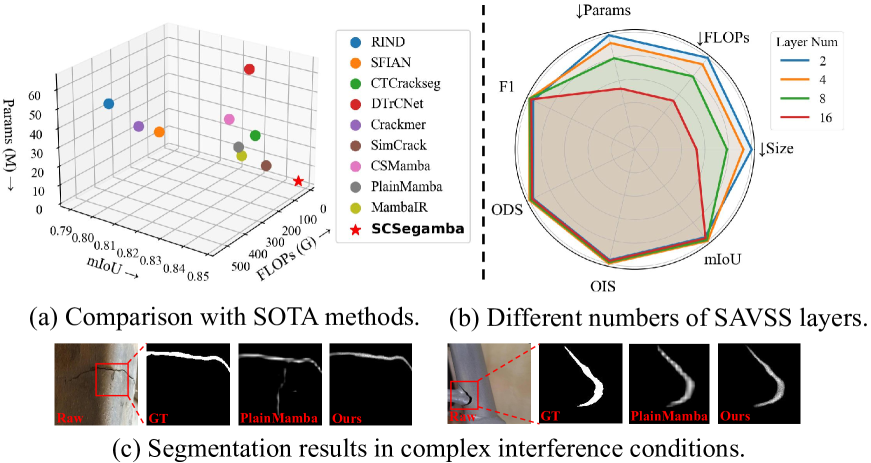
Figure 1: Performance of SCSegamba on multi-scenario TUT [33] dataset. (a) Comparison with SOTA methods. (b) Impact of different SAVSS layer numbers on performance, with normalized metrics; FLOPs (G), Params (M), and Size (MB) decrease towards the edges. (c) Visual results under complex interference.

Structures like bitumen pavement, concrete, and metal frequently develop cracks under shear stress, making regular health monitoring essential to avoid production issues [4, 3, 19, 23, 30]. Due to differences in material properties and environmental conditions, various materials exhibit significant variations in crack morphology and visual appearance [24]. As a result, achieving pixel-level crack segmentation across diverse scenarios remains a complex challenge. Recently, Convolutional Neural Networks (CNNs), such as ECSNet [59] and SFIAN [5], have shown effective crack feature extraction capabilities in segmentation tasks due to their strong local inductive properties. However, their limited receptive field constrains their ability to model broad-scope irregular dependencies across the entire image, resulting in discontinuous segmentation and weak background noise suppression. Although dilated convolution [2] expand the receptive field, their inherent inductive bias still prevents them from fully addressing this issue [58], especially in complex crack patterns with heavy background interference.

The success of Vision Transformer (ViT) [10, 47, 45] has demonstrated Transformer’s effectiveness in capturing irregular pixel dependencies, which is crucial for recognizing complex crack textures, as seen in networks like DTrCNet [48], MFAFNet [9], and Crackmer [46]. However, the quadratic complexity of attention calculations with sequence length leads to high memory use and training challenges for high-resolution images, limiting deployment on resource-constrained edge devices and practical applications. As shown in Figure 1(a), Transformer-based methods like CTCrackseg [44] and DTrCNet [48] perform well, but their large parameter counts and high computational demands limit their deployability on resource-constrained devices. Although variants like Sparse Transformer [6] and Linear Transformer [21] reduce computational requirements by sparsifying or linearizing attention, they sacrifice the ability to model irregular dependencies and pixel textures, hindering pixel-level detection tasks. Consequently, Transformer-based methods struggle to balance segmentation performance with computational efficiency.

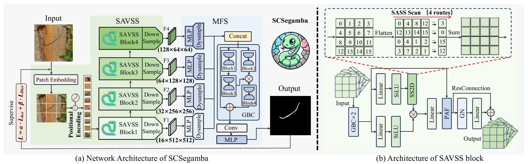
Figure 2: Overview of our proposed method. (a) illustrates the overall architecture of SCSegamba and the processing flow for crack images. (b) displays the structure of the SAVSS block. The input crack image undergoes comprehensive morphological and texture feature extraction through SAVSS, while MFS produces a high-quality pixel-level segmentation map.

Recently, Selective State Space Models (SSMs) have attracted considerable interest due to Mamba’s showing strong performance in sequence modeling while maintaining low computational demands [15, 14]. Vision Mamba (ViM) [62] and VMamba [36] have extended Mamba to the visual domain. The irregular extension of crack regions with numerous branches in low-contrast images, often affected by irrelevant areas and shadows, challenges existing Mamba VSS (Visual State Space Model) block structures and scanning strategies in capturing crack morphology and texture effectively. Most Mamba-based methods [37, 55, 52, 51] process feature maps through linear layers, limiting selective enhancement or suppression of crack features against irrelevant disturbances, thus reducing detailed morphological extraction. Additionally, common parallel or unidirectional diagonal scans [16] struggle to maintain semantic continuity when handling irregular, multi-directional pixel topologies, weakening their ability to manage complex textures and suppress noise. Consequently, current Mamba-based SSM frequently produce false or missed detections in multi-scenario crack images. Moreover, although these methods have the advantage of fewer parameters, there remains potential to further reduce their computational demands and enhance their deployability on edge devices. As shown in Figure 1(b), CSMamba [37], MambaIR [16], and PlainMamba [55] showed unsatisfactory performance on crack images, with room for improvement in parameter count and computational load.

To tackle the challenge of balancing high segmentation quality with low computational demands, we propose the SCSegamba network that produces high-quality pixel-level crack segmentation maps with low computational resources. To improve the Mamba network’s perception of irregular crack textures, we design a Structure-Aware Visual State Space block (SAVSS), employing a Structure-Aware Scanning Strategy (SASS) to enhance semantic continuity and strengthen crack morphology perception. For capturing crack shape cues while maintaining low parameter and computational costs, we designed a lightweight Gated Bottleneck Convolution (GBC) that dynamically adjusts weights for complex backgrounds and varying morphologies. Additionally, the Multi-scale Feature Segmentation head (MFS) integrates the GBC and Multi-layer Perceptron (MLP) to achieve high-quality segmentation maps with low computational requirements. As shown in Figure 1(c), optimal segmentation performance was achieved with four SAVSS layers, producing clear segmentation maps that effectively mask complex interference while maintaining model lightweightness.

In essence, the primary contributions of our work are outlined as follows:

• We propose a novel lightweight vision Mamba network, SCSegamba, for crack segmentation. This model effectively captures morphological and irregular texture cues of crack pixels, using low computational resources to generate high-quality segmentation maps.

• We design the SAVSS with a lightweight GBC Convolution and a SASS scanning strategy to enhance the handling and perception of irregular texture cues in crack images. Additionally, a simple yet effective MFS is developed to generate segmentation maps with relatively low computational resources.

• We evaluate SCSegamba on benchmark datasets across diverse scenarios, with results demonstrating that our method outperforms other SOTA methods while maintaining the low parameter count.

2 Related Works

2.1 Crack Segmentation Network

Early crack detection methods often relied on traditional feature extraction techniques, such as wavelet transform [61], percolation models [54], and the k-means algorithm [25]. Although straightforward to implement, these methods face challenges in suppressing background interference and achieving high segmentation accuracy. With advancements in deep learning, researchers have developed CNN-based crack segmentation networks that achieve SOTA performance [49, 7, 26, 40, 5, 18]. For instance, DeepCrack [35] enables end-to-end pixel-level segmentation, while FPHBN [56] demonstrates strong generalization capabilities. BARNet [17] detects crack boundaries by integrating image gradients with features, and ADDUNet [1] captures both fine and coarse crack characteristics across varied conditions. Although CNN-based methods show significant promise, the local operations and limited receptive fields of CNNs limit their ability to fully capture crack texture cues and effectively suppress background noise.

Transformers [45], with their self-attention mechanism, are well-suited for visual tasks that require long-range dependency modeling, making them increasingly popular in crack segmentation networks [41, 53, 9, 31, 32]. For example, VCVNet [39], based on Vision Transformer (ViT), is designed for bridge crack segmentation, addressing fine-grained segmentation challenges. SWT-CNN [27] combines Swin Transformer and CNN for automatic feature extraction, while TBUNet [60], a Transformer-based knowledge distillation model, achieves high-performance crack segmentation with a hybrid loss function. Although Transformer-based methods are highly effective at capturing crack texture cues and suppressing background noise, their self-attention mechanism introduces computational complexity that grows quadratically with sequence length. This results in a high parameter count and significant computational demands, which limit their deployment on resource-constrained edge devices.

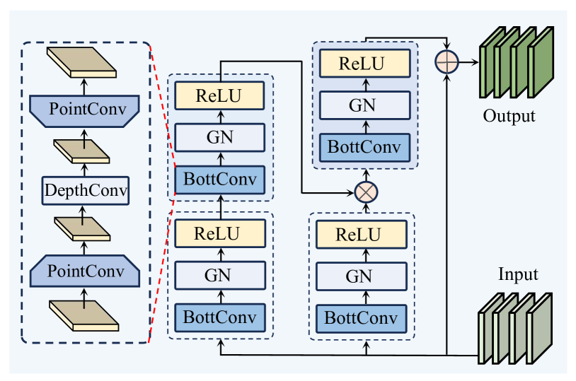
Figure 3: Architecture of GBC. It employs bottleneck convolution to efficiently reduce the parameters and computational load, while the gating mechanism enhances the model’s adaptability in processing diverse crack patterns and complex backgrounds. GN represents group normalization.

2.2 Selective State Space Model

The introduction of the Selective State Space Models (S6) in the Mamba model [14] has highlighted the potential of SSM [12, 13]. Unlike the linear time-invariant S4 model, S6 efficiently captures complex long-distance dependencies while preserving computational efficiency, achieving strong performance in NLP, audio, and genomics. Consequently, researchers have adapted Mamba to the visual domain, creating various VSS blocks. ViM [62] achieves comparable modeling to ViT [10] without attention mechanisms, using fewer computational resources, while VMamba [36] prioritizes efficient computation and high performance. PlainMamba [55] employs a fixed-width layer stacking approach, excelling in tasks such as instance segmentation and object detection. However, the VSS block and scanning strategy require specific optimizations for each visual task, as tasks differ in their reliance on long- and short-distance information, necessitating customized VSS block designs to ensure optimal performance.

Currently, no high-performing Mamba-based model exists for crack segmentation. Thus, designing an optimized VSS structure specifically for crack segmentation is essential to improve performance and efficiency. Given the intricate details and irregular textures of cracks, the VSS block requires strong shape extraction and directional awareness to effectively capture crack texture cues. Additionally, it should facilitate efficient crack segmentation while minimizing computational resource requirements.

3 Methodology

3.1 Preliminary

The complete architecture of our proposed SCSegamba is depicted in Figure 2. It includes two main components: the SAVSS for extracting crack shape and texture cues, and the MFS for efficient feature processing. To capture key crack region cues, we integrate the GBC at the initial stage of SAVSS and the final stage of MFS.

For a single RGB image $E\in\mathbb{R}^{3\times H\times W}$, spatial information is divided into $n$ patches, forming a sequence $\{B_{1},B_{2},\dots,B_{n}\}$. This sequence is processed through the SAVSS block, embedding key crack pixel cues into multi-scale feature maps $\{F_{1},F_{2},F_{3},F_{4}\}$. Finally, in the MFS, all information is consolidated into a single tensor, producing a refined segmentation output $W\in\mathbb{R}^{1\times H\times W}$.

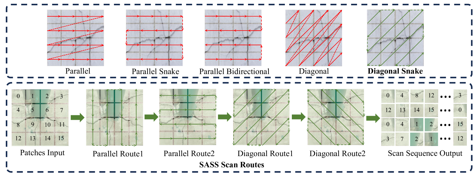
Figure 4: Illustration of our proposed SASS and other scanning strategies. The first row presents four commonly used single scanning paths, along with our proposed diagonal snake path. The second row illustrates the execution flow of our proposed SASS scanning strategy.

3.2 Lightweight Gated Bottleneck Convolution

The gating mechanism enables dynamic features for each spatial position and channel, enhancing the model’s ability to capture details [8, 57]. To further reduce parameter count and computational cost, we embedded a bottleneck convolution (BottConv) with low-rank approximation [28], mapping matrices from high to low dimensional spaces and significantly lowering computational complexity.

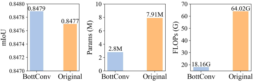
Figure 5: Performance comparison between using BottConv and raw convolution in GBC on the TUT [33] dataset.

In the convolution layer, assuming the spatial size of the filter is $p$, the number of input channels is $d$ and the input is $s$, the convolution response can be represented as:

$$z=Qs+c$$ (1)

where $Q$ is a matrix of size $f\times(p^{2}\times d)$, $f$ is the number of output channels, and $c$ is the original bias term. Assuming $z$ lies in a low-rank subspace of rank $f_{0}$, it can be represented as $z=V(z-z_{1})+z_{1}$, where $z_{1}$ abstracts the mean vector of features, acting as an auxiliary variable to facilitate theoretical derivation and correct feature offsets, $V=LM^{T}$ ($L\in\mathbb{R}^{f\times f_{0}}$, $M\in\mathbb{R}^{(p^{2}d)\times f_{0}}$) represents the low-rank projection matrix. The simplified response then becomes:

$$z=LM^{T}s+c^{\prime}$$ (2)

Since $f_{0}<f$, the computational complexity reduces from $O(fp^{2}d)$ to $O(f_{0}p^{2}d)+O(ff_{0})$, where $O(ff_{0})\ll O(fp^{2}d)$, indicating that the computational complexity reduction is proportional to the original ratio of $f_{0}/f$.

In BottConv, pointwise convolutions project features into or out of low-rank subspace, thus significantly reducing complexity, while depthwise convolution that perform spatial information-adequate extraction in subspace guarantees negligibly low complexity. As shown in Figure 5, BottConv in our GBC design significantly reduces parameter count and computational load compared to the original convolution, with minimal performance impact.

As shown in Figure 3, the input feature $x\in\mathbb{R}^{C\times H\times W}$ is retained as $x_{\text{residual}}=x$ to facilitate the residual connection. Subsequently, the feature $x$ is passed through the BottConv layer, followed by normalization and activation functions, resulting in the features $x_{1}$ and $g_{2}(x)$ as shown below:

$$g_{1}(x)=ReLU(Norm_{1}(f_{1}(x)))$$ (3)

$$x_{1}=ReLU(Norm_{2}(BottConv_{2}(g_{1}(x))))$$ (4)

$$g_{2}(x)=ReLU(Norm_{3}(BottConv_{3}(x)))$$ (5)

To generate the gating feature map, $x_{1}$ and $g_{2}(x)$ are combined through the Hadamard product:

$$m(x)=x_{1}\odot g_{2}(x)$$ (6)

The gating feature map $m(x)$ is subsequently processed through BottConv once again to further refine fine-grained details. After the residual connection is applied, the resulting output is:

$$y=ReLU(Norm_{4}(BottConv_{4}(m(x))))$$ (7)

$$Output=y+x_{residual}$$ (8)

The design of BottConv and deeper gated branch enable the model to preserve basic crack features while dynamically refining the fine-grained feature characterization of the main branch, resulting in more accurate segmentation maps in detailed regions.

3.3 Structure-Aware Visual State Space Module

Our designed SAVSS features a two-dimensional selective scan (SS2D) tailored for visual tasks. Different scanning strategies impact the model’s ability to capture continuous crack textures. As shown in Figure 4, current vision Mamba networks use various scanning directions, including parallel, snake, bidirectional, and diagonal scans [62, 36, 55]. Parallel and diagonal scans lack continuity across rows or diagonals, which limits their sensitivity to crack directions. Although bidirectional and snake scans maintain semantic continuity along horizontal or vertical paths, they struggle to capture diagonal or interwoven textures. To address this, our proposed diagonal snake scanning is designed to better capture complex crack texture cues.

SASS consists of four paths: two parallel snake paths and two diagonal snake paths. This design enables the effective extraction of continuous semantic information in regular crack regions while preserving texture continuity in multiple directions, making it suitable for multi-scenario crack images with complex backgrounds.

After the RGB crack image undergoes Patch Embedding and Position Encoding, it is input as a sequence into the SAVSS block. To maintain a lightweight network, we use only 4 layers of SAVSS blocks. The processing equations are as follows:

$$\overline{P}=e^{\Delta P}$$ (9)

$$\overline{Q}=(\Delta P)^{-1}(e^{\Delta P}-I)\cdot\Delta Q$$ (10)

$$z_{k}=\overline{P}z_{k-1}+\overline{Q}w_{k}$$ (11)

$$u_{k}=Rz_{k}+Sw_{k}$$ (12)

In these equations, the input $w\in\mathbb{R}^{t\times D}$, $P\in\mathbb{R}^{G\times D}$ controls the hidden spatial state, $S\in\mathbb{R}^{D\times D}$ is used to initialize the skip connection for input, $z_{k}$ represents the specific hidden state at time step $k$, and $Q\in\mathbb{R}^{G\times D}$ and $R\in\mathbb{R}^{G\times D}$ are matrices with hidden spatial dimensions $G$ and temporal dimensions $D$, respectively, obtained through selective scanning SS2D. These are trainable parameters that are updated accordingly. $u_{k}$ represents the output at time step $k$. SASS establishes multi-directional adjacency relationships, allowing the hidden state $z_{k}$ to capture more intricate topological and textural details, while enabling the output $u_{k}$ to more effectively integrate multi-directional features.

To effectively combine the initial sequence $x$ with the sequence processed through SS2D, we incorporate Pixel Attention-oriented Fusion (PAF) [33], enhancing SAVSS’s ability to capture crack shape and texture details. Following selective scanning, a residual connection is applied to the fused information to preserve detail and facilitate feature flow. Furthermore, GBC refines the inter-layer output within SAVSS, strengthening crack information extraction and boosting performance in later stages.

3.4 Multi-scale Feature Segmentation Head

Unlike convolutional layers, the MLP swiftly learns the mapping relationships between features and labels, thereby reducing model complexity. When the four feature maps $F_{1},F_{2},F_{3},F_{4}\in\mathbb{R}^{C\times H\times W}$ produced by SAVSS are fed into MFS, they undergo individual processing through the efficient MLP operation and dynamic upsampling [34], restoring their resolution to the original size and yielding $F_{1}^{\text{up}},F_{2}^{\text{up}},F_{3}^{\text{up}},F_{4}^{\text{up}}\in\mathbb{R}^{C\times H\times W}$. The formula is as follows:

$$F_{i}^{up}=DySample(MLP_{i}(F_{i}))$$ (13)

where $i$ denotes the layer index.

To integrate all multi-scale crack shape and texture representations, these feature maps are aggregated into a single tensor, obtaining a high-quality crack segmentation map $o\in\mathbb{R}^{1\times H\times W}$ as follows:

$$o_{1}=GBC(Concat(F_{1}^{up},F_{2}^{up},F_{3}^{up},F_{4}^{up}))$$ (14)

$$o=MLP(Conv(o_{1}))$$ (15)

3.5 Objective Function

We use a blend of Binary Cross-Entropy loss (BCE) [29] and Dice loss [43] as the objective function, which helps improve the network’s robustness to imbalanced pixel data. The overall loss function is expressed as follows:

$$L=\alpha\cdot L_{Dice}+\beta\cdot L_{BCE}$$ (16)

where the hyperparameters $\alpha$ and $\beta$ control the weights of the two loss components. The ratio of $\alpha$ to $\beta$ is set to 1:5.

4 Experiments

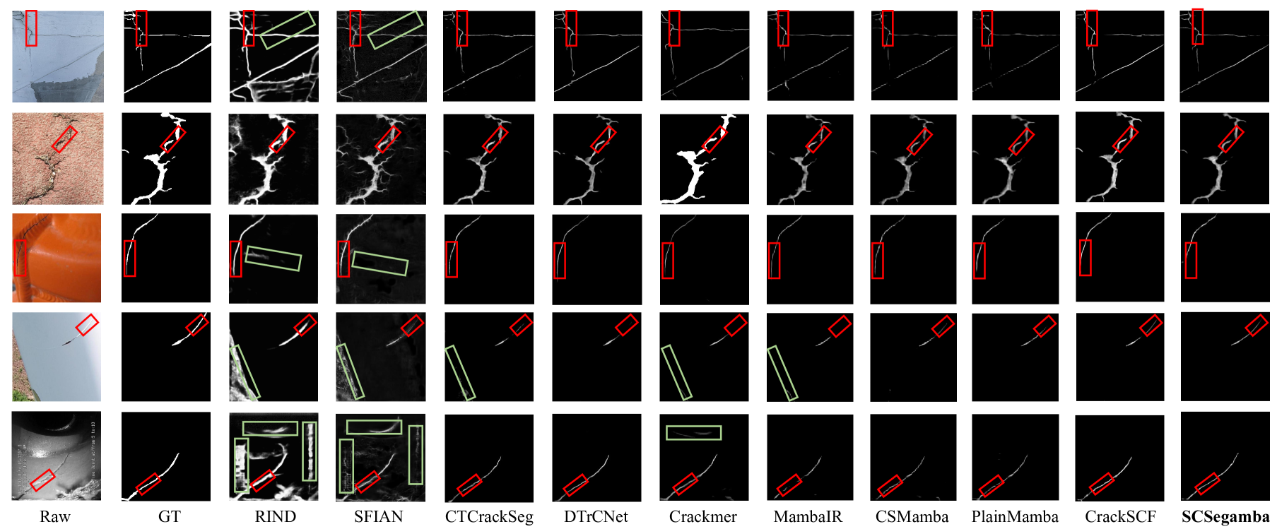
Figure 6: Visual comparison of typical cracks with 9 SOTA methods across four datasets. Red boxes highlight critical details, and green boxes mark misidentified regions.

4.1 Datasets

Crack500 [56] . The images in this dataset were captured using a mobile phone. The original dataset consists of 500 bitumen crack images, which were expanded to 3368 images through data augmentation. Each image is paired with a corresponding pixel-level annotated binary image.

DeepCrack [35] . The dataset comprises 537 RGB images of cement, bricks and bitumen cracks under various conditions, including fine, wide, stained, and fuzzy cracks, ensuring diversity and representativeness.

CrackMap [22] . The dataset was created for a road crack segmentation study and consists of 120 high-resolution RGB images capturing a variety of thin and complex bitumen road cracks.

TUT [33] . In contrast to other datasets with simple backgrounds, this dataset includes a dense, cluttered background and features cracks with elaborate, intricate shapes. It contains 1408 RGB images across eight scenarios: bitumen, cement, bricks, runway, tiles, metal, blades, and pipes.

During processing, all datasets were divided into training, validation, and test sets with a 7:1:2 ratio.

4.2 Implementation Details.

Experimental Settings. We built our SCSegamba network using PyTorch v1.13.1 and trained it on an Intel Xeon Platinum 8336C CPU with eight Nvidia GeForce RTX 4090 GPUs. The AdamW optimizer was used with an initial learning rate of 5e-4, PolyLR scheduling, a weight decay of 0.01, and a random seed of 42. The network was trained for 50 epochs, and the model with the best validation performance was selected for testing.

Comparison Methods. To comprehensively evaluate our model, we compared SCSegamba with 9 SOTA methods. The CNN or Transformer-based models included RIND [38], SFIAN [5], CTCrackSeg [44], DTrCNet [48], Crackmer [46] and SimCrack [20]. Additionally, we compared it with other Mamba-based models, including CSMamba [37], PlainMamba [55], and MambaIR [16].

Evaluation Metrics. We used six metrics to evaluate SCSegamba’s performance: Precision (P), Recall (R), F1 Score ($F1=\frac{2RP}{R+P}$), Optimal Dataset Scale (ODS), Optimal Image Scale (OIS), and mean Intersection over Union (mIoU). ODS measures the model’s adaptability to datasets of varying scales at a fixed threshold m, while OIS evaluates adaptability across image scales at an optimal threshold n. The calculation formulas are as follows:

$$ODS=\max_{m}\frac{2\cdot P_{m}\cdot R_{m}}{P_{m}+R_{m}}$$ (17)

$$OIS=\frac{1}{N}\sum_{i=1}^{N}\max_{n}\frac{2\cdot P_{n,i}\cdot R_{n,i}}{P_{n,i}+R_{n,i}}$$ (18)

mIoU is used to measure the mean proportion of the intersection over union between the ground truth and the predicted results. The calculation is given by the formula:

$$mIoU=\frac{1}{N+1}\sum_{l=0}^{N}\frac{p_{ll}}{\sum_{t=0}^{N}p_{lt}+\sum_{t=0}^{N}p_{tl}-p_{ll}}$$ (19)

where $N$ is the number of classes, which we set as $N=1$; $t$ represents the ground truth, $l$ represents the predicted value, and $p_{tl}$ represents the count of pixels classified as $l$ but belonging to $t$.

Additionally, we evaluated our method’s complexity using three metrics: FLOPs, Params, and Model Size, representing computational complexity, parameter complexity, and memory footprint.

Methods			Crack500						DeepCrack
	ODS	OIS	P	R	F1	mIoU	ODS	OIS	P	R	F1	mIoU
RIND [38]	0.6469	0.6483	0.6998	0.7245	0.7119	0.7381	0.8087	0.8267	0.7896	0.8920	0.8377	0.8391
SFIAN [5]	0.6977	0.7348	0.6983	0.7742	0.7343	0.7604	0.8616	0.8928	0.8549	0.8692	0.8620	0.8776
CTCrackSeg [44]	0.6941	0.7059	0.6940	0.7748	0.7322	0.7591	0.8819	0.8904	0.9011	0.8895	0.8952	0.8925
DTrCNet [48]	0.7012	0.7241	0.6527	0.8280	0.7357	0.7627	0.8473	0.8512	0.8905	0.8251	0.8566	0.8661
Crackmer [46]	0.6933	0.7097	0.6985	0.7572	0.7267	0.7591	0.8712	0.8785	0.8946	0.8783	0.8864	0.8844
SimCrack [20]	0.7127	0.7308	0.7093	0.7984	0.7516	0.7715	0.8570	0.8722	0.8984	0.8549	0.8761	0.8744
CSMamba [37]	0.6931	0.7162	0.6858	0.7823	0.7315	0.7592	0.8738	0.8766	0.9025	0.8863	0.8943	0.8863
PlainMamba [55]	0.7035	0.7173	0.7170	0.7557	0.7358	0.7682	0.8646	0.8668	0.9050	0.8659	0.8850	0.8788
MambaIR [16]	0.7043	0.7189	0.7204	0.7681	0.7435	0.7663	0.8796	0.8840	0.9056	0.8895	0.8975	0.8907
SCSegamba (Ours)	0.7244	0.7370	0.7270	0.7859	0.7553	0.7778	0.8938	0.8990	0.9097	0.9124	0.9110	0.9022
Methods			CrackMap						TUT
	ODS	OIS	P	R	F1	mIoU	ODS	OIS	P	R	F1	mIoU
RIND [38]	0.6745	0.6943	0.6023	0.7586	0.6699	0.7425	0.7531	0.7891	0.7872	0.7665	0.7767	0.8051
SFIAN [5]	0.7200	0.7465	0.6715	0.7668	0.7160	0.7748	0.7290	0.7513	0.7715	0.7367	0.7537	0.7896
CTCrackSeg [44]	0.7289	0.7373	0.6911	0.7669	0.7270	0.7785	0.7940	0.7996	0.8202	0.8195	0.8199	0.8301
DTrCNet [48]	0.7328	0.7413	0.6912	0.7681	0.7276	0.7812	0.7987	0.8073	0.7972	0.8441	0.8202	0.8331
Crackmer [46]	0.7395	0.7437	0.7229	0.7467	0.7346	0.7860	0.7429	0.7640	0.7501	0.7656	0.7578	0.7966
SimCrack [20]	0.7559	0.7625	0.7380	0.7672	0.7523	0.7963	0.7984	0.8090	0.8051	0.8371	0.8208	0.8334
CSMamba [37]	0.7371	0.7413	0.7053	0.7663	0.7346	0.7841	0.7879	0.7946	0.7947	0.8353	0.8146	0.8263
PlainMamba [55]	0.7150	0.7189	0.6649	0.7616	0.7099	0.7699	0.7867	0.7967	0.7701	0.8523	0.8102	0.8253
MambaIR [16]	0.7332	0.7347	0.7569	0.7013	0.7280	0.7834	0.7861	0.7930	0.7877	0.8387	0.8125	0.8249
SCSegamba (Ours)	0.7741	0.7766	0.7629	0.7727	0.7678	0.8094	0.8204	0.8255	0.8241	0.8545	0.8390	0.8479

Table 1: Comparison with 9 SOTA methods across 4 datasets. Best results are in bold, and second-best results are underlined.

Methods	Year	FLOPs↓	Params↓	Size↓
RIND [38]	2021	695.77G	59.39M	453MB
SFIAN [5]	2023	84.57G	13.63M	56MB
CTCrackSeg [44]	2023	39.47G	22.88M	174MB
DTrCNet [48]	2023	123.20G	63.45M	317MB
Crackmer [46]	2024	14.94G	5.90M	43MB
SimCrack [20]	2024	286.62G	29.58M	225MB
CSMamba [37]	2024	145.84G	35.95M	233MB
PlainMamba [55]	2024	73.36G	16.72M	96MB
MambaIR [16]	2024	47.32G	10.34M	79MB
SCSegamba (Ours)	2024	18.16G	2.80M	37MB

Table 2: Comparison of complexity with other methods. Best results are in bold, and second-best results are underlined.

Seg Head	ODS	OIS	P	R	F1	mIoU	Params ↓	FLOPs ↓	Model Size ↓
UNet [42]	0.8055	0.8151	0.8148	0.8376	0.8260	0.8378	2.92M	19.27G	39MB
Ham [11]	0.7703	0.7784	0.7962	0.7838	0.7909	0.8124	2.86M	35.08G	38MB
SegFormer [50]	0.7947	0.7983	0.8170	0.8174	0.8172	0.8307	2.79M	17.87G	35MB
MFS	0.8204	0.8255	0.8241	0.8545	0.8390	0.8479	2.80M	18.16G	37MB

Table 3: Ablation study of different segmentation heads. UNet [42], Ham [11], and SegFormer [50] are high-performance heads.

GBC	PAF	Res	ODS	OIS	P	R	F1	mIoU	Params ↓	FLOPs ↓	Model Size ↓
2713	2717	2717	0.8136	0.8196	0.8213	0.8461	0.8335	0.8434	2.49M	16.75G	34MB
2717	2713	2717	0.7998	0.8084	0.7918	0.8524	0.8222	0.8343	2.28M	14.91G	33MB
2717	2717	2713	0.7936	0.8069	0.7952	0.8438	0.8197	0.8313	2.48M	15.65G	35MB
2713	2713	2717	0.8047	0.8102	0.8174	0.8379	0.8275	0.8377	2.54M	17.08G	35MB
2713	2717	2713	0.8116	0.8200	0.8156	0.8522	0.8334	0.8425	2.75M	17.82G	37MB
2717	2713	2713	0.8023	0.8076	0.8219	0.8302	0.8260	0.8360	2.54M	15.99G	35MB
2713	2713	2713	0.8204	0.8255	0.8241	0.8545	0.8390	0.8479	2.80M	18.16G	37MB

Table 4: Ablation study of components within the SAVSS block. Best results are in bold, and second-best results are underlined.

4.3 Comparison with SOTA Methods

As listed in Table 1, compared with 9 other SOTA methods, our proposed SCSegamba achieves the best performance across four public datasets. Specifically, on the Crack500 [56] and DeepCrack [35] datasets, which contain larger and more complex crack regions, SCSegamba achieved the highest performance. Notably, on the DeepCrack dataset, it surpassed the next best method by 1.50% in F1 score and 1.09% in mIoU. This improvement is due to the robust ability of GBC to capture morphological clues in large crack areas, enhancing the model’s representational power. On the CrackMap [22] dataset, which features thinner and more elongated cracks, our method surpasses all other SOTA methods in every metric, outperforming the next best method by 2.06% in F1 and 1.65% in mIoU. This demonstrates the effectiveness of SASS in capturing fine textures and elongated crack structures. As illustrated in Figure 6, our method produces clearer and more precise feature maps, with superior detail capture in typical scenarios such as cement and bitumen, compared to other methods.

For the TUT dataset [33], which includes eight diverse scenarios, our method achieved the best performance, surpassing the next best method by 2.21% in F1 and 1.74% in mIoU. As shown in Figure 6, whether in the complex crack topology of plastic tracks, the noise-heavy backgrounds of metallic materials and turbine blades, or the low-contrast, dimly lit underground pipeline images, SCSegamba consistently produced high-quality segmentation maps while effectively suppressing irrelevant noise. This demonstrates that our method, with the enhanced crack morphology and texture perception from GBC and SASS, exhibits exceptional robustness and stability. Additionally, leveraging MFS for feature aggregation improves multi-scale perception, making our model particularly suited for diverse, interference-rich scenarios.

4.4 Complexity Analysis

Table 2 shows a comparison of the complexity of our method with other SOTA methods when the input image size is uniformly set to 512. With only 2.80M parameters and a model size of 37MB, our method surpasses all others, being 52.54% and 13.95% lower than the next best result, respectively. Additionally, compared to Crackmer [46], which prioritizes computational efficiency, our method’s FLOPs are only 3.22G higher. This demonstrates that the combination of lightweight SAVSS and MFS enables high-quality segmentation in noisy crack scenes with minimal parameters and low computational load, which is essential for resource-constrained devices.

4.5 Ablation Studies

We performed ablation experiments on the representative multi-scenario dataset TUT [33].

Ablation study of segmentation heads. As listed in Table 3, with our designed MFS, SCSegamba achieved the best results across all six metrics, with F1 and mIoU scores 1.57% and 1.21% higher than the second-best method. In terms of complexity, although Params, FLOPs, and Model Size are only 0.01M, 0.29G, and 2MB larger than the SegFormer head, our method surpasses it in F1 and mIoU by 2.67% and 2.07%, respectively. This demonstrates that MFS enhances SAVSS output integration, significantly improving performance while keeping the model lightweight.

Scan	ODS	OIS	P	R	F1	mIoU
Parallel	0.8123	0.8184	0.8146	0.8523	0.8330	0.8427
Diag	0.8091	0.8148	0.8225	0.8417	0.8320	0.8410
ParaSna	0.8102	0.8162	0.8219	0.8365	0.8291	0.8408
DiagSna	0.8153	0.8215	0.8237	0.8497	0.8365	0.8451
SASS	0.8204	0.8255	0.8241	0.8545	0.8390	0.8479

Table 5: Ablation studies with different four-route scanning strategies in the SAVSS block, comparing parallel, diagonal, parallel snake, and diagonal snake scanning. The impact of different scanning strategies on complexity is negligible; thus, complexity analysis is omitted from this table. Best results are in bold, and second-best results are underlined.

Ablation study of components. Table 4 shows the impact of each component in SAVSS on model performance. When fully utilizing GBC, PAF, and residual connections, our model achieved the best results across all metrics. Notably, adding GBC led to significant improvements in F1 and mIoU by 1.57% and 1.42%, respectively, highlighting its strength in capturing crack morphology cues. Similarly, residual connections boosted F1 and mIoU by 0.13% and 2.47%, indicating their role in focusing on essential crack features. Although using only PAF resulted in the lowest Params, FLOPs, and Model Size, it significantly reduced performance. These findings demonstrate that our fully integrated SAVSS effectively captures crack morphology and texture cues, achieving top pixel-level segmentation results while maintaining a lightweight model.

Ablation studies of scanning strategies. As listed in Table 5, under the same conditions of using four different directional scanning paths, the model achieved the best performance with our designed SASS scanning strategy, improving F1 and mIoU by 0.30% and 0.33% over the diagonal snake strategy. This demonstrates SASS’s ability to construct semantic and dependency information suited to crack topology, enhancing crack pixel perception in subsequent modules. More comprehensive experiments and real-world deployments are available in the Appendix.

5 Conclusion

In this paper, we proposed SCSegamba, a lightweight structure-aware Vision Mamba for precise pixel-level crack segmentation. SCSegamba combines SAVSS and MFS to enhance crack shape and texture perception with a low parameter count. Equipped with GBC and SASS scanning, SAVSS, captures irregular crack textures across various structures. Experiments on four datasets show SCSegamba’s exceptional performance, especially in complex, noisy scenarios. On the challenging multi-scenario dataset, it achieved an F1 score of 0.8390 and mIoU of 0.8479 with only 18.16G FLOPs and 2.8M parameters, demonstrating its effectiveness for real-world crack detection and suitability for edge devices. Future work will incorporate multimodal cues to enhance segmentation quality, while further optimizing VSS design and scan strategies to achieve high-quality results with low computational resources.

6 Acknowledgement

This work was supported by the National Natural Science Foundation of China (NSFC) under Grants 62272342, 62020106004, 62306212, and T2422015; the Tianjin Natural Science Foundation under Grants 23JCJQJC00070 and 24PTLYHZ00320; and the Marie Skłodowska-Curie Actions (MSCA) under Project No. 101111188.

Supplementary Material

7 Details of SASS and Ablation Experiments

As described in Subsection 3.3, the SASS strategy enhances semantic capture in complex crack regions by scanning texture cues from multiple directions. SASS combines parallel snake and diagonal snake scans, aligning the scanning paths with the actual extension and irregular shapes of cracks, ensuring comprehensive capture of texture information.

To evaluate the necessity of using four scanning paths in SASS, we conducted ablation experiments with different path numbers across various scanning strategies on multi-scenario dataset TUT. As listed in Table 6, all strategies performed significantly better with four paths than with two, likely because four paths allow SAVSS to capture finer crack details and topological cues. Notably, aside from SASS, the diagonal snake-like scan consistently achieved the second-best results, with two-path configurations yielding F1 and mIoU scores 0.48% and 0.45% higher than the diagonal unidirectional scan. This indicates that the diagonal snake-like scan provides more continuous semantic information, enhancing segmentation. Importantly, our proposed SASS achieved the best results with both two-path and four-path setups, demonstrating its effectiveness in capturing diverse crack topologies.

To clarify the implementation of our proposed SASS, we present its execution process in Algorithm 1.

Parallel	N	ODS	OIS	P	R	F1	mIoU
	2	0.8032	0.8126	0.7994	0.8474	0.8231	0.8365
	4	0.8123	0.8184	0.8146	0.8523	0.8330	0.8427
PaSna	2	0.8035	0.8124	0.8062	0.8458	0.8258	0.8369
	4	0.8102	0.8162	0.8219	0.8365	0.8291	0.8408
Diag	2	0.8080	0.8166	0.8058	0.8496	0.8271	0.8408
	4	0.8091	0.8148	0.8225	0.8417	0.8320	0.8410
DigSna	2	0.8094	0.8162	0.8185	0.8470	0.8325	0.8413
	4	0.8153	0.8215	0.8237	0.8497	0.8365	0.8451
SASS	2	0.8130	0.8192	0.8196	0.8478	0.8335	0.8430
	4	0.8204	0.8255	0.8241	0.8545	0.8390	0.8479

Table 6: Ablation study on the number of paths in different scanning strategies. N represents the number of paths. For two-path scans, SASS uses the first parallel snake and diagonal snake scans, while other methods use the first two paths. Best results are in bold, and second-best results are underlined.

$\alpha$ : $\beta$	ODS	OIS	P	R	F1	mIoU
BCE	0.8099	0.8151	0.8207	0.8457	0.8330	0.8414
Dice	0.8022	0.8072	0.8038	0.8430	0.8231	0.8358
5 : 1	0.8125	0.8168	0.8207	0.8432	0.8319	0.8428
4 : 1	0.8144	0.8184	0.8217	0.8442	0.8328	0.8437
3 : 1	0.8180	0.8229	0.8293	0.8436	0.8364	0.8463
2 : 1	0.8098	0.8152	0.8204	0.8392	0.8297	0.8408
1 : 1	0.8123	0.8184	0.8141	0.8507	0.8320	0.8423
1 : 2	0.8152	0.8214	0.8210	0.8484	0.8345	0.8443
1 : 3	0.8109	0.8163	0.8226	0.8396	0.8310	0.8418
1 : 4	0.8133	0.8185	0.8163	0.8515	0.8336	0.8433
1 : 5	0.8204	0.8255	0.8241	0.8545	0.8390	0.8479

Table 7: Sensitivity analysis experiments with different $\alpha$ and $\beta$ ratios. Best results are in bold, and second-best results are underlined.

8 Details of Objective Function and Analysis

The calculation formulas for BCE [29] loss and Dice [43] loss are as follows:

$$L_{Dice}=1-\frac{2\sum_{j=1}^{M}p_{j}\hat{p}_{j}+\epsilon}{\sum_{j=1}^{M}p_{j}+\sum_{j=1}^{M}\hat{p}_{j}+\epsilon}$$ (20)

$$L_{BCE}=-\frac{1}{N}\left[p_{j}\log(\hat{p}_{j})+(1-p_{j})\log(1-\hat{p}_{j})\right]$$ (21)

where $M$ denotes the number of samples, $p_{j}$ is the ground truth label for the $j$-th sample, $\hat{p}_{j}$ is the predicted probability for the $j$-th sample, $\epsilon$ is a small constant.

In equation 16, the ratio of $\alpha$ to $\beta$ is set to 1:5. This is the optimal ratio of $\alpha$ and $\beta$ selected after experimenting with various hyperparameter settings on multi-scenario dataset. As listed in Table 7, setting the $\alpha$ to $\beta$ ratio at 1:5 yields the best performance, with improvements of 0.65% in F1 and 0.55% in mIoU over the 1:2 ratio. This suggests that balancing Dice and BCE loss at a 1:5 ratio helps the model better distinguish background pixels from the few crack region pixels, thereby enhancing performance.

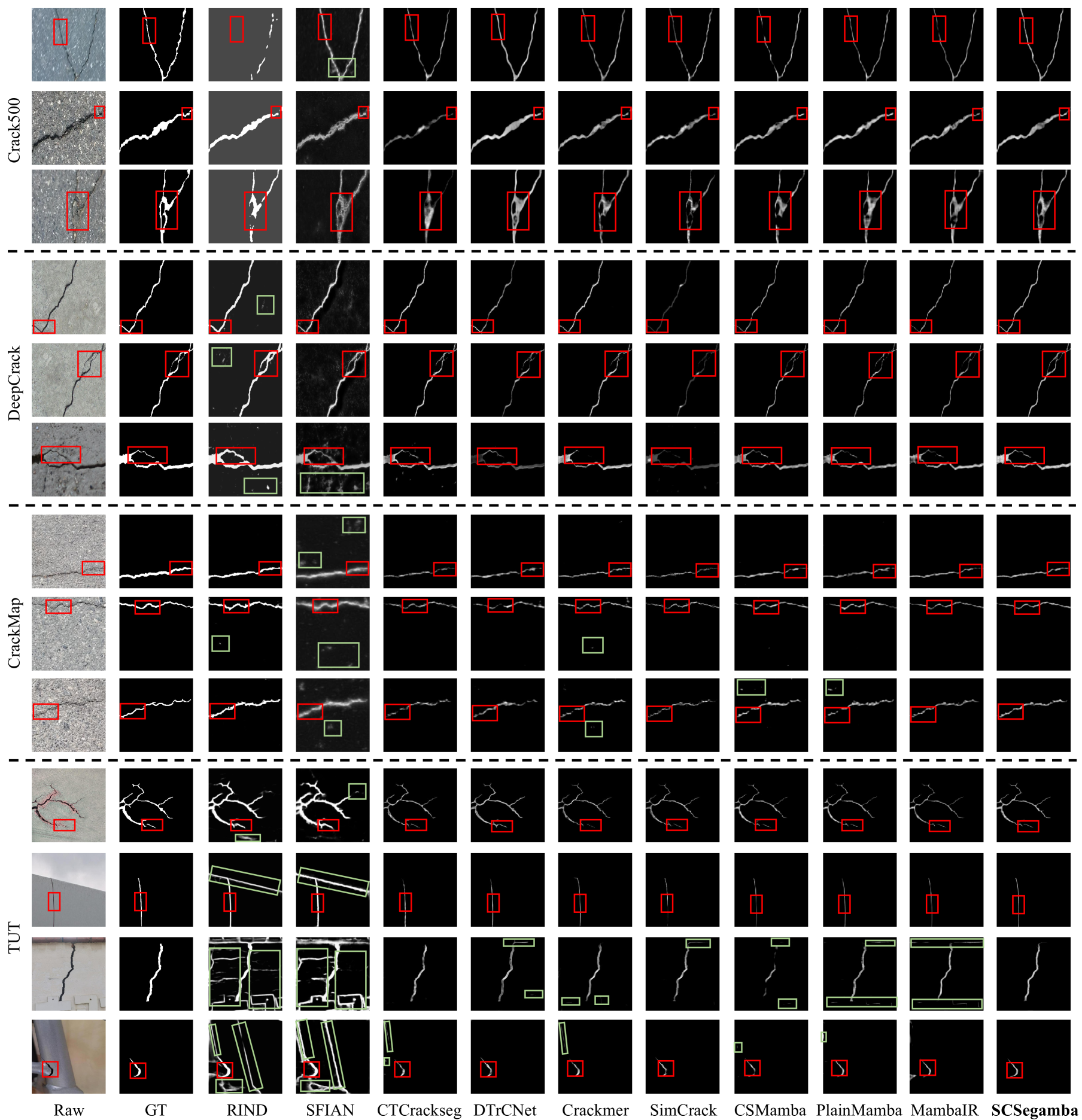
Figure 7: Visual comparison with 9 SOTA methods across four public datasets. Red boxes highlight critical details, and green boxes mark misidentified regions.

Layer Num	ODS	OIS	P	R	F1	mIoU	Params ↓	FLOPs ↓	Model Size ↓
2	0.8102	0.8165	0.8181	0.8420	0.8299	0.8413	1.56M	12.26G	20MB
4	0.8204	0.8255	0.8241	0.8545	0.8390	0.8479	2.80M	18.16G	37MB
8	0.8174	0.8222	0.8199	0.8579	0.8387	0.8461	5.23M	29.27G	68MB
16	0.8126	0.8187	0.8226	0.8475	0.8349	0.8430	10.08M	51.51G	127MB
32	0.5203	0.5365	0.5830	0.5680	0.5754	0.6785	19.79M	95.97G	247MB

Table 8: Experiments with different numbers of SAVSS layers. Best results are in bold, and second-best results are underlined.

Patch Size	ODS	OIS	P	R	F1	mIoU	Params ↓	FLOPs ↓	Model Size ↓
4	0.8053	0.8128	0.8146	0.8443	0.8294	0.8381	2.61M	51.81G	34MB
8	0.8204	0.8255	0.8241	0.8545	0.8390	0.8479	2.80M	18.16G	37MB
16	0.7910	0.7937	0.8126	0.8141	0.8133	0.8272	3.59M	9.74G	45MB
32	0.7318	0.7364	0.7535	0.7576	0.7555	0.7879	6.74M	7.64G	82MB

Table 9: Experiments with different patch sizes. Best results are in bold, and second-best results are underlined.

Methods	ODS	OIS	P	R	F1	mIoU	Params ↓	FLOPs ↓	Model Size ↓
MambaIR [16]	0.7869	0.7956	0.7714	0.8445	0.8071	0.8240	3.57M	19.71G	29MB
CSMamba [37]	0.7140	0.7201	0.6934	0.8171	0.7503	0.7773	12.68M	15.44G	84MB
PlainMamba [55]	0.7787	0.7896	0.7617	0.8531	0.8064	0.8201	2.20M	14.09G	18MB
SCSegamba (Ours)	0.8204	0.8255	0.8241	0.8545	0.8390	0.8479	2.80M	18.16G	37MB

Table 10: Comparison experiments of different Mamba-based methods using 4 VSS layers. Best results are in bold, and second-best results are underlined.

9 Visualisation Comparisons

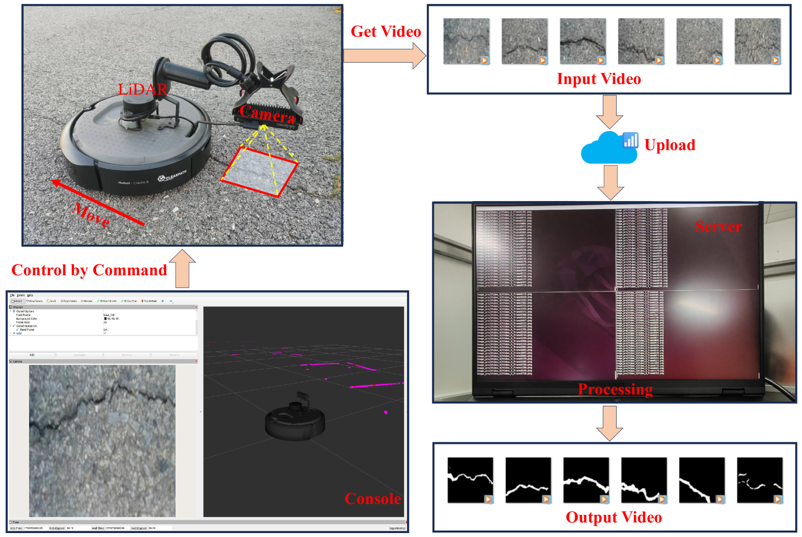
Figure 8: Schematic of real-world deployment. The intelligent vehicle is placed on an outdoor road surface, and we use the server terminal to remotely control it. The vehicle transmits the video data in real-time to the server, where it is processed to obtain the final output.

To visually demonstrate the advantages of SCSegamba, we present detailed visual results in Figure 7. For the Crack500 [56], DeepCrack [35], and CrackMap [22] datasets, which primarily include bitumen, concrete, and brick scenarios with minimal background noise and a range of crack thicknesses, our method consistently achieves accurate segmentation, even capturing intricate fine cracks. This is attributed to GBC’s strong capability in capturing crack morphology. In contrast, other methods show weaker performance in continuity and fine segmentation, resulting in discontinuities and expanded segmentation areas that do not align with actual crack images.

For the TUT [33] dataset, which includes diverse scenarios and significant background noise, our method excels at suppressing interference. For instance, in images of cracks on generator blades and steel pipes, it effectively minimizes irrelevant noise and provides precise crack segmentation. This performance is largely attributed to SAVSS’s accurate capture of crack topologies. In contrast, CNN-based methods like RIND [38] and SFIAN [5] struggle to distinguish background noise from crack regions, highlighting their limitations in contextual dependency capture. Other Transformer and Mamba-based methods also fall short in segmentation continuity and detail handling compared to our approach.

10 Additional Analysis

To provide a thorough demonstration of the necessity of each component in our proposed SCSegamba, we conducted a more extensive analysis experiment.

Comparison with different numbers of SAVSS layers. In our SCSegamba, we used 4 layers of SAVSS blocks to balance performance and computational requirements. As listed in Table 8, 4 layers achieved optimal results, with F1 and mIoU scores 0.036% and 0.21% higher than with 8 layers, while reducing parameters by 2.43M, computation by 11.11G, and model size by 31MB. Although using only 2 layers minimized resource demands, with 1.56M parameters, performance decreased. Conversely, using 32 layers increased resource use and reduced performance due to redundant features, which impacted generalization. Thus, 4 SAVSS layers strike an effective balance between performance and resource efficiency, making it ideal for practical applications.

Comparison with different Patch Size. In our SAVSS, we set the Patch Size to 8 during Patch Embedding. To verify its effectiveness, we conducted experiments with various Patch Sizes. As listed in Table 9, a Patch Size of 8 yields the best performance, with F1 and mIoU scores 1.16% and 1.17% higher than a Patch Size of 4. Although a smaller Patch Size of 4 reduces parameters and model size, it limits the receptive field and hinders the effective capture of longer textures, impacting segmentation. As shown in Figure 9, as the Patch Size increases, parameter count and model size decrease, but the computational load per patch rises, affecting efficiency. At a Patch Size of 32, performance drops significantly due to reduced fine-grained detail capture and sensitivity to contextual variations. Thus, a Patch Size of 8 balances detail accuracy and generalization while maintaining model efficiency.

Comparison under the same number of VSS layers. In Subsection 4.3, we compare SCSegamba with other SOTA methods, using default VSS layer settings for Mamba-based models like MambaIR [16], CSMamba [37], and PlainMamba [55]. To examine complexity and performance under uniform VSS layer counts, we set all Mamba-based models to 4 VSS layers and conducted comparisons. As listed in Table 2 and 10, although computational requirements for MambaIR, CSMamba, and PlainMamba decrease, their performance drops significantly. For example, CSMamba’s F1 and mIoU scores drop to 0.7503 and 0.7773. While PlainMamba with 4 layers achieves reductions of 0.60M in parameters, 4.07G in FLOPs, and 19MB in model size, SCSegamba surpasses it by 4.04% in F1 and 3.39% in mIoU. Thus, with 4 SAVSS layers, SCSegamba balances performance and efficiency, capturing crack morphology and texture for high-quality segmentation.

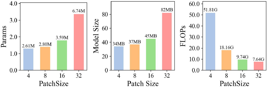
Figure 9: Comparison of computing resources required for different Patch Size

11 Real-world Deployment Applications

To validate the effectiveness of our proposed SCSegamba in real-world applications, we conducted a practical deployment and compared its real-world performance with other SOTA methods. Specifically, our experimental system consists of two main components: the intelligent vehicle and the server. The intelligent vehicle used is a Turtlebot4 Lite driven by a Raspberry Pi 4, equipped with a LiDAR and a camera. The camera model is OAK-D-Pro, fitted with an OV9282 image sensor capable of capturing high-quality crack images. The server is a laptop equipped with a Core i9-13900 CPU running Ubuntu 22.04. The intelligent vehicle and server communicate via the internet. This setup simulates resource-limited equipment to evaluate the performance of our SCSegamba in real-world deployment scenarios.

Methods	Inf Time↓
RIND [38]	0.0909s
SFIAN [5]	0.0286s
CTCrackseg [44]	0.0357s
DTrCNet [48]	0.0213s
Crackmer [46]	0.0323s
SimCrack [20]	0.0345s
CSMamba [37]	0.0625s
PlainMamba [55]	0.1667s
MambaIR [16]	0.0400s
SCSegamba (Ours)	0.0313s

Table 11: Comparison of inference time with other SOTA methods on resource-constrained server.

As shown in Figure 8, in the real-world deployment process, the intelligent vehicle was placed on an outdoor road surface filled with cracks. We remotely controlled the vehicle from the server terminal, directing it to move forward in a straight line at a speed of 0.15 m/s. The camera captured video at a frame rate of 30 frames per second. The vehicle transmitted the recorded video data to the server in real-time via the network. To accelerate data transmission from the vehicle to the server, we set the recording resolution to 512 × 512. Upon receiving the video data, the server first segmented it into frames, then fed each frame into the pre-trained SCSegamba model, which was trained on all datasets, for inference. After segmentation, the server recombined the processed frames into a video, yielding the final output. This setup simulates real-time crack segmentation in an real-world production process.

Additionally, we deployed the weight files of other SOTA methods on the server for comparison. As listed in Table 11, our SCSegamba achieved an inference speed of 0.0313 seconds per frame on the resource-constrained server, outperforming most other methods. This demonstrates that our method has excellent real-time performance, making it suitable for real-time segmentation of cracks in video data.

As shown in Figure 10, compared to other SOTA methods, our SCSegamba better suppresses irrelevant noise in video data and generates continuous crack region segmentation maps. For instance, although SSM-based methods like PlainMamba [55], MambaIR [16], and CSMamba [37] achieve continuous segmentation, they tend to produce false positives in some irrelevant noise spots. Additionally, while CNN and Transformer-based methods achieve high metrics and performance on datasets with faster inference speed, their performance on video data is suboptimal, often showing discontinuous segmentation and poor background suppression. For example, cracks segmented by DTrCNet [48] and CTCrackSeg [44] exhibit significant discontinuities, and Crackmer [46] struggles to distinguish between crack and background regions. Based on the above real-world deployment results, our SCSegamba produces high-quality segmentation results on crack video data with low parameters and computational resources, making it more suitable for deployment on resource-constrained devices and demonstrating its strong performance in practical production scenarios.

Algorithm 1 SASS execution process

1:  Input: Patch matrix dimensions $H$, $W$

2:  Output: $O=(o1,o2,o3,o4)$, $O\_inverse=(o1\_inverse,o2\_inverse,o3\_inverse,o4\_inverse)$, $D=(d1,d2,d3,d4)$

3:  Initialize: $L=H\times W$

4:  Initialize $(i,j)\leftarrow(0,0)$ for $o1$, $(H-1,W-1)$ if $H$ is odd else $(H-1,0)$ for $o2$

5:  $i_{d}\leftarrow down$, $j_{d}\leftarrow left$ if $H$ is odd else $right$

6:  while $j<W$ or $i\geq 0$ do

7:   $idx\leftarrow i\times W+j$, append $idx$ to $o1$, set $o1\_inverse[idx]$

8:   if $i_{d}=down$ and $i<H-1$ then

9:    $i\leftarrow i+1$, add $down$ to $d1$

10:   else

11:    $j\leftarrow j+1$, $i_{d}\leftarrow up$ if $i=H-1$ else $down$, add $right$ to $d1$

12:   end if

13:   $idx\leftarrow i\times W+j$, append $idx$ to $o2$, set $o2\_inverse[idx]$

14:   if $j_{d}=right$ and $j<W-1$ then

15:    $j\leftarrow j+1$, add $right$ to $d2$

16:   else

17:    $i\leftarrow i-1$, $j_{d}\leftarrow left$ if $j=W-1$ else $right$, add $up$ to $d2$

18:   end if

19:  end while

20:  $d1\leftarrow[d_{start}]+d1[:-1]$, $d2\leftarrow[d_{start}]+d2[:-1]$

21:  for $\text{diag}\leftarrow 0$ to $H+W-2$ do

22:   $direction\leftarrow right$ if diag is even else $down$

23:   for $k\leftarrow 0$ to $\min(\text{diag}+1,H,W)-1$ do

24:    $i,j\leftarrow(\text{diag}-k,k)$ if diag is even else $(k,\text{diag}-k)$

25:    if $j<W$ then

26:     $idx\leftarrow i\times W+j$

27:     Append $idx$ to $o3$, set $o3\_inverse[idx]$, add $direction$ to $d3$

28:    end if

29:    $i,j\leftarrow(\text{diag}-k,W-k-1)$ if diag is even else $(k,W-\text{diag}+k-1)$

30:    if $j<W$ then

31:     $idx\leftarrow i\times W+j$

32:     Append $idx$ to $o4$, set $o4\_inverse[idx]$, add $direction$ to $d4$

33:    end if

34:   end for

35:  end for

36:  $d3\leftarrow[d_{start}]+d3[:-1]$, $d4\leftarrow[d_{start}]+d4[:-1]$

37:  Return: $O$, $O\_inverse$, $D$

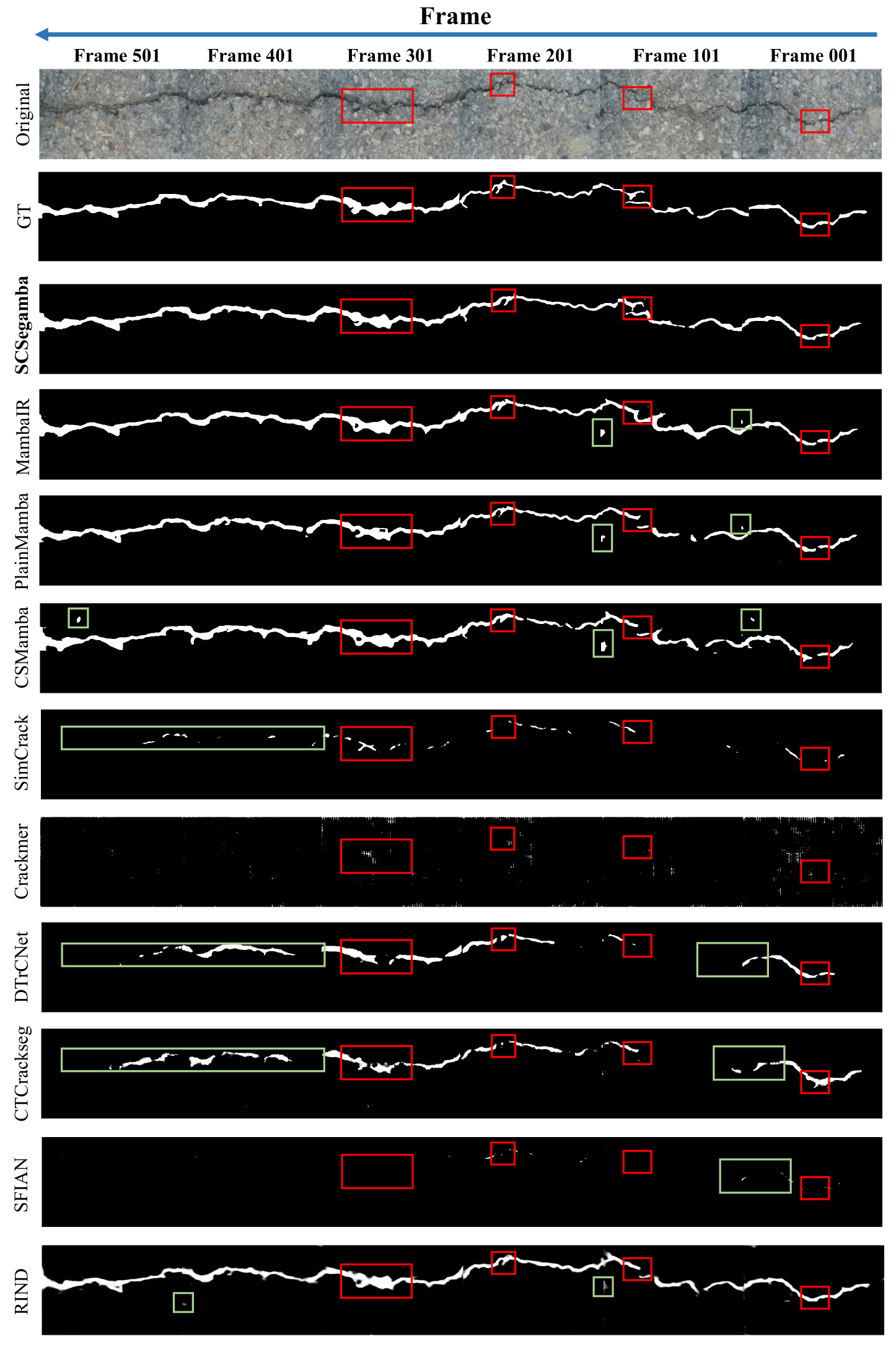
Figure 10: Visualisation comparison on video data keyframes. The interval between keyframes is 100 frames in order to ensure continuity of observation. Red boxes highlight critical details, and green boxes mark misidentified regions.

References

- Al-Huda et al. [2023] Zaid Al-Huda, Bo Peng, Riyadh Nazar Ali Algburi, Mugahed A Al-antari, AL-Jarazi Rabea, Omar Al-maqtari, and Donghai Zhai. Asymmetric dual-decoder-u-net for pavement crack semantic segmentation. Automation in Construction, 156:105138, 2023.
- Chen et al. [2018] Liang-Chieh Chen, Yukun Zhu, George Papandreou, Florian Schroff, and Hartwig Adam. Encoder-decoder with atrous separable convolution for semantic image segmentation. In Proceedings of the European conference on computer vision, pages 801–818, 2018.
- Chen et al. [2022] Zhuangzhuang Chen, Jin Zhang, Zhuonan Lai, Jie Chen, Zun Liu, and Jianqiang Li. Geometry-aware guided loss for deep crack recognition. In Proceedings of the IEEE/CVF Conference on Computer Vision and Pattern Recognition, pages 4703–4712, 2022.
- Chen et al. [2024] Zhuangzhuang Chen, Zhuonan Lai, Jie Chen, and Jianqiang Li. Mind marginal non-crack regions: Clustering-inspired representation learning for crack segmentation. In Proceedings of the IEEE/CVF Conference on Computer Vision and Pattern Recognition, pages 12698–12708, 2024.
- Cheng et al. [2023] Xu Cheng, Tian He, Fan Shi, Meng Zhao, Xiufeng Liu, and Shengyong Chen. Selective feature fusion and irregular-aware network for pavement crack detection. IEEE Transactions on Intelligent Transportation Systems, 2023.
- Child et al. [2019] Rewon Child, Scott Gray, Alec Radford, and Ilya Sutskever. Generating long sequences with sparse transformers. arXiv preprint arXiv:1904.10509, 2019.
- Choi and Cha [2019] Wooram Choi and Young-Jin Cha. Sddnet: Real-time crack segmentation. IEEE Transactions on Industrial Electronics, 67(9):8016–8025, 2019.
- Dauphin et al. [2017] Yann N Dauphin, Angela Fan, Michael Auli, and David Grangier. Language modeling with gated convolutional networks. In International conference on machine learning, pages 933–941. PMLR, 2017.
- Dong et al. [2024] Jiaxiu Dong, Niannian Wang, Hongyuan Fang, Wentong Guo, Bin Li, and Kejie Zhai. Mfafnet: An innovative crack intelligent segmentation method based on multi-layer feature association fusion network. Advanced Engineering Informatics, 62:102584, 2024.
- Dosovitskiy et al. [2021] Alexey Dosovitskiy, Lucas Beyer, Alexander Kolesnikov, Dirk Weissenborn, Xiaohua Zhai, Thomas Unterthiner, Mostafa Dehghani, Matthias Minderer, Georg Heigold, Sylvain Gelly, Jakob Uszkoreit, and Neil Houlsby. An image is worth 16x16 words: Transformers for image recognition at scale. In The International Conference on Learning Representations, 2021.
- Geng et al. [2021] Zhengyang Geng, Meng-Hao Guo, Hongxu Chen, Xia Li, Ke Wei, and Zhouchen Lin. Is attention better than matrix decomposition? In International Conference on Learning Representations, 2021.
- Goel et al. [2022] Karan Goel, Albert Gu, Chris Donahue, and Christopher Ré. It’s raw! audio generation with state-space models. In International Conference on Machine Learning, pages 7616–7633. PMLR, 2022.
- Gu et al. [2022a] Albert Gu, Karan Goel, Ankit Gupta, and Christopher Ré. On the parameterization and initialization of diagonal state space models. Advances in Neural Information Processing Systems, 35:35971–35983, 2022a.
- Gu et al. [2022b] Albert Gu, Karan Goel, and Christopher Ré. Efficiently modeling long sequences with structured state spaces. In The International Conference on Learning Representations, 2022b.
- Gu et al. [2022c] Albert Gu, Karan Goel, and Christopher Ré. Efficiently modeling long sequences with structured state spaces. In The International Conference on Learning Representations, 2022c.
- Guo et al. [2024] Hang Guo, Jinmin Li, Tao Dai, Zhihao Ouyang, Xudong Ren, and Shu-Tao Xia. Mambair: A simple baseline for image restoration with state-space model. In European Conference on Computer Vision, pages 222–241. Springer, 2024.
- Guo et al. [2021] Jing-Ming Guo, Herleeyandi Markoni, and Jiann-Der Lee. Barnet: Boundary aware refinement network for crack detection. IEEE Transactions on Intelligent Transportation Systems, 23(7):7343–7358, 2021.
- He et al. [2016] Kaiming He, Xiangyu Zhang, Shaoqing Ren, and Jian Sun. Deep residual learning for image recognition. In Proceedings of the IEEE conference on computer vision and pattern recognition, pages 770–778, 2016.
- Hsieh and Tsai [2020] Yung-An Hsieh and Yichang James Tsai. Machine learning for crack detection: Review and model performance comparison. Journal of Computing in Civil Engineering, 34(5):04020038, 2020.
- Jaziri et al. [2024] Achref Jaziri, Martin Mundt, Andres Fernandez, and Visvanathan Ramesh. Designing a hybrid neural system to learn real-world crack segmentation from fractal-based simulation. In Proceedings of the IEEE/CVF Winter Conference on Applications of Computer Vision, pages 8636–8646, 2024.
- Katharopoulos et al. [2020] Angelos Katharopoulos, Apoorv Vyas, Nikolaos Pappas, and François Fleuret. Transformers are rnns: Fast autoregressive transformers with linear attention. In International conference on machine learning, pages 5156–5165. PMLR, 2020.
- Katsamenis et al. [2023] Iason Katsamenis, Eftychios Protopapadakis, Nikolaos Bakalos, Andreas Varvarigos, Anastasios Doulamis, Nikolaos Doulamis, and Athanasios Voulodimos. A few-shot attention recurrent residual u-net for crack segmentation. In International Symposium on Visual Computing, pages 199–209. Springer, 2023.
- Kheradmandi and Mehranfar [2022] Narges Kheradmandi and Vida Mehranfar. A critical review and comparative study on image segmentation-based techniques for pavement crack detection. Construction and Building Materials, 321:126162, 2022.
- Lang et al. [2024] Hong Lang, Ye Yuan, Jiang Chen, Shuo Ding, Jian John Lu, and Yong Zhang. Augmented concrete crack segmentation: Learning complete representation to defend background interference in concrete pavements. IEEE Transactions on Instrumentation and Measurement, 2024.
- Lattanzi and Miller [2014] David Lattanzi and Gregory R Miller. Robust automated concrete damage detection algorithms for field applications. Journal of Computing in Civil Engineering, 28(2):253–262, 2014.
- Lei et al. [2024] Qin Lei, Jiang Zhong, and Chen Wang. Joint optimization of crack segmentation with an adaptive dynamic threshold module. IEEE Transactions on Intelligent Transportation Systems, 2024.
- Li et al. [2024a] Huaiyuan Li, Hui Li, Chuang Li, Baohai Wu, and Jinghuai Gao. Hybrid swin transformer-cnn model for pore-crack structure identification. IEEE Transactions on Geoscience and Remote Sensing, 2024a.
- Li et al. [2024b] Jialin Li, Qiang Nie, Weifu Fu, Yuhuan Lin, Guangpin Tao, Yong Liu, and Chengjie Wang. Lors: Low-rank residual structure for parameter-efficient network stacking. In Proceedings of the IEEE/CVF Conference on Computer Vision and Pattern Recognition, pages 15866–15876, 2024b.
- Li et al. [2024c] Qiufu Li, Xi Jia, Jiancan Zhou, Linlin Shen, and Jinming Duan. Rediscovering bce loss for uniform classification. arXiv preprint arXiv:2403.07289, 2024c.
- Liao et al. [2022] Jianghai Liao, Yuanhao Yue, Dejin Zhang, Wei Tu, Rui Cao, Qin Zou, and Qingquan Li. Automatic tunnel crack inspection using an efficient mobile imaging module and a lightweight cnn. IEEE Transactions on Intelligent Transportation Systems, 23(9):15190–15203, 2022.
- Liu et al. [2021] Huajun Liu, Xiangyu Miao, Christoph Mertz, Chengzhong Xu, and Hui Kong. Crackformer: Transformer network for fine-grained crack detection. In Proceedings of the IEEE/CVF International Conference on Computer Vision (ICCV), pages 3783–3792, 2021.
- Liu et al. [2023a] Huajun Liu, Jing Yang, Xiangyu Miao, Christoph Mertz, and Hui Kong. Crackformer network for pavement crack segmentation. IEEE Transactions on Intelligent Transportation Systems, 24(9):9240–9252, 2023a.
- Liu et al. [2024a] Hui Liu, Chen Jia, Fan Shi, Xu Cheng, Mianzhao Wang, and Shengyong Chen. Staircase cascaded fusion of lightweight local pattern recognition and long-range dependencies for structural crack segmentation. arXiv preprint arXiv:2408.12815, 2024a.
- Liu et al. [2023b] Wenze Liu, Hao Lu, Hongtao Fu, and Zhiguo Cao. Learning to upsample by learning to sample. In Proceedings of the IEEE/CVF International Conference on Computer Vision, pages 6027–6037, 2023b.
- Liu et al. [2019] Yahui Liu, Jian Yao, Xiaohu Lu, Renping Xie, and Li Li. Deepcrack: A deep hierarchical feature learning architecture for crack segmentation. Neurocomputing, 338:139–153, 2019.
- Liu et al. [2024b] Yue Liu, Yunjie Tian, Yuzhong Zhao, Hongtian Yu, Lingxi Xie, Yaowei Wang, Qixiang Ye, and Yunfan Liu. Vmamba: Visual state space model. arXiv preprint arXiv:2401.10166, 2024b.
- Mushui et al. [2024] Liu Mushui, Jun Dan, Ziqian Lu, Yunlong Yu, Yingming Li, and Xi Li. Cm-unet: Hybrid cnn-mamba unet for remote sensing image semantic segmentation. arXiv preprint arXiv:2405.10530, 2024.
- Pu et al. [2021] Mengyang Pu, Yaping Huang, Qingji Guan, and Haibin Ling. Rindnet: Edge detection for discontinuity in reflectance, illumination, normal and depth. In Proceedings of the IEEE/CVF international conference on computer vision, pages 6879–6888, 2021.
- Qi et al. [2024] Haochen Qi, Xiangwei Kong, Zhibo Jin, Jiqiang Zhang, and Zinan Wang. A vision-transformer-based convex variational network for bridge pavement defect segmentation. IEEE Transactions on Intelligent Transportation Systems, 2024.
- Qu et al. [2021] Zhong Qu, Wen Chen, Shi-Yan Wang, Tu-Ming Yi, and Ling Liu. A crack detection algorithm for concrete pavement based on attention mechanism and multi-features fusion. IEEE Transactions on Intelligent Transportation Systems, 23(8):11710–11719, 2021.
- Quan et al. [2023] Jianing Quan, Baozhen Ge, and Min Wang. Crackvit: a unified cnn-transformer model for pixel-level crack extraction. Neural Computing and Applications, 35(15):10957–10973, 2023.
- Ronneberger et al. [2015] Olaf Ronneberger, Philipp Fischer, and Thomas Brox. U-net: Convolutional networks for biomedical image segmentation. In Medical image computing and computer-assisted intervention–MICCAI 2015: 18th international conference, Munich, Germany, October 5-9, 2015, proceedings, part III 18, pages 234–241. Springer, 2015.
- Sudre et al. [2017] Carole H Sudre, Wenqi Li, Tom Vercauteren, Sebastien Ourselin, and M Jorge Cardoso. Generalised dice overlap as a deep learning loss function for highly unbalanced segmentations. In Deep Learning in Medical Image Analysis and Multimodal Learning for Clinical Decision Support: Third International Workshop, DLMIA 2017, and 7th International Workshop, ML-CDS 2017, Held in Conjunction with MICCAI 2017, pages 240–248. Springer, 2017.
- Tao et al. [2023] Huaqi Tao, Bingxi Liu, Jinqiang Cui, and Hong Zhang. A convolutional-transformer network for crack segmentation with boundary awareness. In 2023 IEEE International Conference on Image Processing, pages 86–90. IEEE, 2023.
- Vaswani [2017] A Vaswani. Attention is all you need. Advances in Neural Information Processing Systems, 2017.
- Wang et al. [2024] Jin Wang, Zhigao Zeng, Pradip Kumar Sharma, Osama Alfarraj, Amr Tolba, Jianming Zhang, and Lei Wang. Dual-path network combining cnn and transformer for pavement crack segmentation. Automation in Construction, 158:105217, 2024.
- Xia et al. [2024] Chunlong Xia, Xinliang Wang, Feng Lv, Xin Hao, and Yifeng Shi. Vit-comer: Vision transformer with convolutional multi-scale feature interaction for dense predictions. In Proceedings of the IEEE/CVF Conference on Computer Vision and Pattern Recognition, pages 5493–5502, 2024.
- Xiang et al. [2023] Chao Xiang, Jingjing Guo, Ran Cao, and Lu Deng. A crack-segmentation algorithm fusing transformers and convolutional neural networks for complex detection scenarios. Automation in Construction, 152:104894, 2023.
- Xiao et al. [2018] Xiao Xiao, Shen Lian, Zhiming Luo, and Shaozi Li. Weighted res-unet for high-quality retina vessel segmentation. In 2018 9th international conference on information technology in medicine and education, pages 327–331. IEEE, 2018.
- Xie et al. [2021] Enze Xie, Wenhai Wang, Zhiding Yu, Anima Anandkumar, Jose M Alvarez, and Ping Luo. Segformer: Simple and efficient design for semantic segmentation with transformers. Advances in neural information processing systems, 34:12077–12090, 2021.
- Xie et al. [2024] Xinyu Xie, Yawen Cui, Tao Tan, Xubin Zheng, and Zitong Yu. Fusionmamba: Dynamic feature enhancement for multimodal image fusion with mamba. Visual Intelligence, 2(1):37, 2024.
- Xing et al. [2024] Zhaohu Xing, Tian Ye, Yijun Yang, Guang Liu, and Lei Zhu. Segmamba: Long-range sequential modeling mamba for 3d medical image segmentation. In International Conference on Medical Image Computing and Computer-Assisted Intervention, pages 578–588. Springer, 2024.
- Xu et al. [2024] Kangmin Xu, Liang Liao, Jing Xiao, Chaofeng Chen, Haoning Wu, Qiong Yan, and Weisi Lin. Boosting image quality assessment through efficient transformer adaptation with local feature enhancement. In Proceedings of the IEEE/CVF Conference on Computer Vision and Pattern Recognition, pages 2662–2672, 2024.
- Yamaguchi et al. [2008] Tomoyuki Yamaguchi, Shingo Nakamura, Ryo Saegusa, and Shuji Hashimoto. Image-based crack detection for real concrete surfaces. IEEJ Transactions on Electrical and Electronic Engineering, 3(1):128–135, 2008.
- Yang et al. [2024] Chenhongyi Yang, Zehui Chen, Miguel Espinosa, Linus Ericsson, Zhenyu Wang, Jiaming Liu, and Elliot J Crowley. Plainmamba: Improving non-hierarchical mamba in visual recognition. arXiv preprint arXiv:2403.17695, 2024.
- Yang et al. [2019] Fan Yang, Lei Zhang, Sijia Yu, Danil Prokhorov, Xue Mei, and Haibin Ling. Feature pyramid and hierarchical boosting network for pavement crack detection. IEEE Transactions on Intelligent Transportation Systems, 21(4):1525–1535, 2019.
- Yu et al. [2019] Jiahui Yu, Zhe Lin, Jimei Yang, Xiaohui Shen, Xin Lu, and Thomas S Huang. Free-form image inpainting with gated convolution. In Proceedings of the IEEE/CVF international conference on computer vision, pages 4471–4480, 2019.
- Zhang et al. [2024] Hang Zhang, Allen A Zhang, Zishuo Dong, Anzheng He, Yang Liu, You Zhan, and Kelvin CP Wang. Robust semantic segmentation for automatic crack detection within pavement images using multi-mixing of global context and local image features. IEEE Transactions on Intelligent Transportation Systems, 2024.
- Zhang et al. [2023] Tianjie Zhang, Donglei Wang, and Yang Lu. Ecsnet: An accelerated real-time image segmentation cnn architecture for pavement crack detection. IEEE Transactions on Intelligent Transportation Systems, 2023.
- Zhang and Huang [2024] Xiaohu Zhang and Haifeng Huang. Distilling knowledge from a transformer-based crack segmentation model to a light-weighted symmetry model with mixed loss function for portable crack detection equipment. Symmetry, 16(5):520, 2024.
- Zhou et al. [2006] Jian Zhou, Peisen S Huang, and Fu-Pen Chiang. Wavelet-based pavement distress detection and evaluation. Optical Engineering, 45(2):027007–027007, 2006.
- Zhu et al. [2024] Lianghui Zhu, Bencheng Liao, Qian Zhang, Xinlong Wang, Wenyu Liu, and Xinggang Wang. Vision mamba: Efficient visual representation learning with bidirectional state space model. In International Conference on Machine Learning, 2024.