A Dynamic Model of Private Asset Allocation

Abstract

We build a state-of-the-art dynamic model of private asset allocation that considers five key features of private asset markets: (1) the illiquid nature of private assets, (2) timing lags between capital commitments, capital calls, and eventual distributions, (3) time-varying business cycle conditions, (4) serial correlation in observed private asset returns, and (5) regulatory constraints on certain institutional investors’ portfolio choices. We use cutting-edge machine learning methods to quantify the optimal investment policies over the life cycle of a fund. Moreover, our model offers regulators a tool for precisely quantifying the trade-offs when setting risk-based capital charges.

JEL classification: C63, G11, G23.

Key words: alternative assets, business cycle, liquidity, machine learning, portfolio choice, private equity, return smoothing, risk-based capital.

1 Introduction

Recent estimates put the size of global private markets’ assets under management at $13.1 trillion as of June 30, 2023 (McKinsey & Company, 2024). A multitude of factors make private asset allocation decisions particularly challenging. First, the illiquid nature of private assets means that it takes considerable time and costs to establish, rebalance, and exit from a position, making careful long-term planning an integral part of private asset management. Second, this illiquidity can lead to mark-to-market induced serial correlation in observed private asset returns, which further complicates dynamic allocation decisions. Third, private market investments require investors to first commit capital and subsequently manage the liquidity needs arising from future capital calls. Fourth, some institutional investors such as insurance companies face additional regulatory constraints on their allocation choices. Fifth, investors must take all of these factors into account as market and business cycle conditions constantly change.

We develop a state-of-the-art dynamic model of private asset allocation. It captures (1) the illiquidity inherent in private asset investing, (2) the lag between initial capital commitments, subsequent capital calls, and eventual distributions, (3) time-varying market and business cycle conditions, (4) serial correlation in observed alternative asset returns, and (5) regulation-induced portfolio constraints. The interplay among these factors introduces substantial nonlinearities and expands the state space, rendering the model numerically intractable with traditional solution methods. To address this challenge, we use advanced machine learning techniques—Deep Kernel Gaussian Processes (Wilson, Hu, Salakhutdinov, and Xing, 2016)—to solve the underlying dynamic programming problem. The solution quantifies the optimal private asset allocation policies over the life cycle of a fund, and accounts for the multitude of factors described above. To the best of our knowledge, (i) our model is the most comprehensive private asset allocation model to date in terms of the range of factors considered, and (ii) we are the first to use Deep Kernel Gaussian Processes in the context of solving dynamic models in economics and finance.

We solve a dynamic portfolio optimization problem for a risk-averse limited partner (LP) investor with a fixed (but long) horizon. The LP chooses among stocks, bonds, and a private equity (PE) fund, subject to various constraints. To invest in the PE fund, the LP must first make capital commitments before capital is called and distributed from the PE fund. The illiquid nature of PE assets makes liquidity management central: the LP must finance capital calls out of its liquid wealth (i.e., stocks and bonds). Default occurs if the LP does not have sufficient liquid wealth to meet a capital call, in which case the LP’s PE stake is sold at a discount on the secondary market and the LP loses future access to the PE fund. In addition to such liquidity-driven defaults, we also allow for strategic defaults on capital calls.

Our model further incorporates three realistic features that make PE investing challenging. First, a unique feature of alternative investments is the serial correlation in observed returns (Geltner, 1991; Getmansky, Lo, and Makarov, 2004). As Getmansky, Lo, and Makarov (2004) argue, sparsely-traded illiquid assets can lead to reported PE fund returns that appear smoother than their true economic counterparts, owing to mark-to-market practices. To capture this effect, we embed the Getmansky, Lo, and Makarov (2004) return-smoothing model into our PE return structure, allowing observed PE returns to depend on past lags of true economic returns. Consequently, the LP must make allocation decisions in the presence of mark-to-market induced smoothing, as is the case in reality.

Second, key determinants of PE investing depend on business cycle conditions. For example, PE returns, capital calls, and distributions can all vary over the business cycle (see, e.g., Neuberger Berman 2022). We capture these time-varying conditions by modeling a macroeconomic state that evolves according to a Markov chain. All our model parameters, including those governing PE returns, call rates, and distributions, can depend on this macroeconomic state. Consequently, our framework provides guidance for optimal PE allocations over different phases of the business cycle.

Third, many PE investors are institutional investors that must comply with regulatory constraints on their asset holdings. For example, U.S. insurers’ portfolio allocations are governed by Risk-Based Capital (RBC) standards overseen by the National Association of Insurance Commissioners (NAIC), while European insurers are subject to analogous RBC requirements under Solvency II (see Eling and Holzmuller 2008 for an overview of RBC standards). Violations of these requirements can be extremely costly because they trigger regulatory interventions: in severe cases, an insurer may be placed under regulatory control, which can lead to rehabilitation or even liquidation. We capture these regulatory constraints by imposing a risk budget on the LP’s portfolio, applying separate risk charges to stocks, bonds, and PE. As long as the LP’s total risk charge remains below a specified threshold, no costs arise; however, costs escalate once that threshold is breached. This modeling approach aligns with risk-charge frameworks commonly used by rating agencies to assess insurers’ RBC adequacy (see, e.g., S&P Global 2023).

The comprehensive set of factors considered in our model makes it challenging to solve the LP’s dynamic portfolio optimization problem for two main reasons. First, the interactions among these factors introduce substantial nonlinearities that must be resolved to obtain accurate allocation policies. Second, they enlarge the state space, making traditional methods infeasible due to their vulnerability to the curse of dimensionality.

To overcome these challenges, we employ Deep Kernel Gaussian Processes (DKGPs) to track the LP’s value and policy functions within our dynamic optimization framework. As proposed by Wilson, Hu, Salakhutdinov, and Xing (2016), DKGPs combine the strengths of Gaussian Processes (GPs) and Neural Networks (NNs). While both GPs and NNs can address high-dimensional challenges, GPs are generally more cost-effective to train since they involve fewer hyperparameters. This is especially relevant in our setting where each sample point requires solving a constrained optimization problem with multi-dimensional controls and adaptive quadrature to accurately compute expectations. However, standard GPs often lack the flexibility of NNs in capturing complex nonlinear behavior. DKGPs resolve this issue by embedding NNs into GPs, thereby harnessing the ability to model highly nonlinear dynamics while reducing the need for expensive sample points. While we use DKGPs to solve our model, this methodology may be of independent interest, as many models in economics and finance face similar challenges.

Our calibration assumes a 10-year investment horizon for the LP, and we use private equity (PE) data from Liberty Mutual Investments to calibrate our model. The calibrated model yields several quantitative insights into optimal asset allocation over a fund’s life cycle—from the initial stage, where no PE investments are held, to the transition phase, during which the LP ramps up its PE exposure, and finally to the maintenance stage, where the desired balance between PE and public investments is achieved.

First, the optimal allocation policy unfolds as follows. In the early years, the LP aggressively commits new capital to build up the fund, taking into account the various factors described above to ensure a smooth transition. At the same time, the LP adjusts its liquid portfolio by initially allocating heavily to stocks to achieve the desired overall aggregate risk exposure as PE investments ramp up. As PE commitments are called and the PE share of the portfolio increases, the LP gradually reduces stock exposure. This transition phase lasts approximately 4–5 years, after which the LP enters a maintenance phase, consistently managing the portfolio to preserve the optimal asset mix. Notably, under the optimal policy, the cumulative default rate is only 0.1% over the ten-year investment horizon.

Although similar outcomes are observed in practice, the complexity of the problem has traditionally led practitioners to rely on heuristics. For instance, standard approaches often use static mean-variance analysis combined with heuristic adjustments for capital commitment lags (see, e.g., Takahashi and Alexander 2002). Our contribution is to rigorously quantify the optimal policies in a realistic setting, moving beyond rules of thumb to help PE investors achieve improved outcomes. Indeed, we demonstrate that the optimal portfolio allocations obtained under our fully dynamic framework can differ dramatically from those derived using heuristic methods.

Second, the optimal allocation accounts for business cycle conditions as follows. To first order, the optimal allocation maintains the intended transition profile for the PE portfolio, as if short-term business cycle fluctuations did not exist. This is because adjusting PE allocations can be prohibitively costly given their illiquidity, commitment lags, and long planning horizons. Instead, the LP modulates overall risk exposure over the business cycle by adjusting its public stock holdings, lowering exposure during recessions when necessary. Since transaction costs for public stocks are negligible in comparison, this approach offers a cost-effective means of managing risk over the business cycle.

Failing to account for business cycles is extremely costly. To quantify these costs, we compare the outcomes for a naive LP that ignores business cycle variation against outcomes under the optimal policy. The naive LP adopts overly aggressive PE allocations, leading to a dramatic increase in default risk: the cumulative default frequency is 13.6% for the naive approach, compared to only 0.1% under the optimal policy. Ex-ante, this suboptimal strategy translates to a 9.3% loss in initial wealth in certainty-equivalent terms.

Third, we examine whether it is necessary to “unsmooth” returns before making allocation decisions. Prior research has argued that mark-to-market accounting induces serial correlation, making observed alternative asset returns appear smoother than their underlying true economic performance (Getmansky, Lo, and Makarov, 2004). This smoothing can cause private assets’ true risk to be underestimated and, consequently, lead to suboptimal portfolio allocations. As a result, some have advocated unsmoothing returns prior to drawing portfolio inferences.

Our model revisits this issue from the perspective of a long-term PE investor and demonstrates that the need to unsmooth returns may be a moot point for such an investor. The reasons are as follows. First, long-term investors care primarily about the characteristics of long-horizon returns, which are less affected by short-term mark-to-market fluctuations. Second, even if serial correlation is an inherent feature of true PE returns, its benefits may be negated once realistic implementation lags and adjustment costs are considered. Indeed, in our baseline calibration—where observed PE returns have a quarterly autocorrelation of 0.2—we observe little difference in outcomes between a LP that optimizes its portfolio directly using the raw returns and one that first unsmooths the return series to remove autocorrelation while preserving the long-run moments.

Fourth, our model can be used to evaluate the impact of varying risk charges on the LP’s portfolio outcomes by quantifying the associated risk–return trade-off. In our baseline calibration, we impose a 50% risk charge on both public and private equities, reflecting representative industry figures (see, e.g., S&P Global 2023, Table 14). Because these charges differ across asset classes, we also consider a scenario in which the risk charge is increased to 100%, near the upper end of observed ranges. Under this higher risk charge scenario, the calibrated model indicates that long-run realized returns decline from 8.4% to 7.1%, while long-run realized volatility decreases from 2.78% to 2.35%. These findings underscore how our framework can help both institutional investors and regulators assess the cost and benefits of alternative risk-charge levels.

Related literature.

We contribute to two strands of literature. First, we advance the research on optimal private asset allocation (see, e.g., Korteweg and Westerfield (2022) for a recent survey). Early industry approaches to estimating exposures and cash flows include Takahashi and Alexander (2002). More recent work has focused on dynamic models with stochastic shocks, and highlight two key features of private asset investing: the inherent illiquidity of these assets (Ang, Papanikolaou, and Westerfield, 2014; Sorensen, Wang, and Yang, 2014; Dimmock, Wang, and Yang, 2024) and the delays between capital commitments, calls, and distributions (Giommetti and Sorensen, 2024; Gourier, Phalippou, and Westerfield, 2024). We build on these prior works by incorporating additional factors that pose significant challenges for PE investors, including time-varying business cycle conditions, serial correlation in observed PE returns, and regulation-induced portfolio constraints. To the best of our knowledge, our model is the most comprehensive stochastic model of private asset allocation to date.

Second, we contribute to a growing literature that uses machine learning methods to tackle portfolio choice problems featuring higher dimensions, realistic trading frictions, and complex constraints. Most of this work has focused on liquid asset markets such as stocks and government bonds (see, e.g., Gaegauf, Scheidegger, and Trojani 2023; Duarte, Duarte, and Silva 2024), leaving alternative asset classes like private equity understudied in comparison—despite their rising importance in institutional portfolios. Our contribution is to extend machine learning techniques to the alternative asset allocation setting, enabling us to characterize optimal private asset allocation under a range of realistic features. To the best of our knowledge, we are the first to deploy Deep Kernel Gaussian Processes for solving dynamic models in economics and finance. This methodological advance is of independent interest, as similar challenges frequently arise in various settings in economics and finance. For example, Duarte, Fonseca, Goodman, and Parker (2022) apply neural networks to a portfolio choice problem in the household context that incorporates multiple realistic features. While their methodology characterizes optimal portfolio choice under full commitment, our approach instead characterizes the optimal time-consistent policy.

2 Model

Time is discrete and runs from $t=0$ to the terminal date $t=T$. The limited partner (LP) investor maximizes utility over terminal wealth $W_{T}$,

$$u\left(W_{T}\right)=\frac{W_{T}^{1-\gamma}}{1-\gamma},$$ (1)

where $\gamma$ is the coefficient of relative risk aversion. At each time period $t$, the LP can invest in a risk-free bond, a public stock index, and private equity (PE). The timing of the decisions is illustrated in Figure˜1 and is described below.

Time-varying macroeconomic conditions.

The LP’s investment opportunities set varies over the business cycle. We capture time-varying business cycle conditions through a Markov process $s_{t}\in\{1,2\}$ that takes two values corresponding to recessions ($s_{t}=1$) and booms ($s_{t}=2$). We denote by $p_{ss^{\prime}}=\mbox{prob}(s_{t+1}=s^{\prime}|s_{t}=s)$ the probability of transitioning from state $s$ to state $s^{\prime}$.

Liquidity constraint.

The LP enters period $t$ with liquid wealth $W_{t}\geq 0$, uncalled PE commitments $K_{t}\geq 0$, and illiquid wealth $P_{t}\geq 0$. The latter corresponds to the net asset value (NAV) of the LP’s previously called PE investments. The LP then makes three choices: (1) new PE commitments $N_{t}\geq 0$, and its allocations to (2) stocks $S_{t}$ and (3) bonds $B_{t}$. These choices are subject to the following liquidity constraint:

$$S_{t}+B_{t}+\gamma_{N}(W_{t}+P_{t})\left(\frac{N_{t}}{W_{t}+P_{t}}-\overline{n}\right)^{2}+\gamma_{S}(W_{t}+P_{t})\left(\frac{S_{t}}{W_{t}+P_{t}}-\overline{s}\right)^{2}=W_{t}$$ (2)

where $\gamma_{N}(W_{t}+P_{t})\left(\frac{N_{t}}{W_{t}+P_{t}}-\overline{n}\right)^{2}$ and $\gamma_{S}(W_{t}+P_{t})\left(\frac{S_{t}}{W_{t}+P_{t}}-\overline{s}\right)^{2}$ are adjustment costs on new PE commitments and stocks, respectively. That is, stock and bond allocations and adjustment costs are paid out of liquid wealth.

Additionally, we show in Appendix B that solvency concerns rule out shorting so that

$$B_{t}\geq 0,\quad\quad S_{t}\geq 0.$$ (3)

Figure 1: Timing of the Model

Risk budget.

The LP’s overall portfolio is subject to internal risk controls which we model through risk weights. Specifically, the risk weight of the LP’s overall portfolio is defined as

$$\theta_{t}=\frac{\theta_{B}B_{t}+\theta_{S}\left[S_{t}+\gamma_{S}(W_{t}+P_{t})\left(\frac{S_{t}}{W_{t}+P_{t}}\right)^{2}\right]+\theta_{P}P_{t}}{B_{t}+S_{t}+\gamma_{S}(W_{t}+P_{t})\left(\frac{S_{t}}{W_{t}+P_{t}}\right)^{2}+P_{t}}$$ (4)

The interpretation of the risk weight (4) is as follows. The LP’s combined portfolio consists of $B_{t}$ invested in bonds, $S_{t}+\gamma_{S}(W_{t}+P_{t})\left(\frac{S_{t}}{W_{t}+P_{t}}\right)^{2}$ in stocks (including stock adjustment costs), and $P_{t}$ in PE. Bonds carry a risk weight of $\theta_{B}$, while stocks and PE carry risk weights of $\theta_{S}$ and $\theta_{P}$, respectively. The risk weight (4) is the value-weighted average over the risk weights of the three classes of investments in the LP’s portfolio. We assume the risk weights are ordered as follows:

$$0=\theta_{B}<\theta_{S}\leq\theta_{P}.$$ (5)

That is, risk-free bonds carry a zero risk weight as they are risk free while public stocks and PE carry positive risk weights. The risk weight for PE is no lower than that of public stocks.

The LP incurs a cost if it violates its risk budget. Specifically, the cost of violating its risk budget equals $\left(W_{t}+P_{t}\right)\times\Gamma\left(\theta_{t}\right)$ where the proportional cost equals

$$\Gamma\left(\theta_{t}\right)=\kappa\left(\theta_{t}-\overline{\theta}\right)^{2}1_{\left\{\theta_{t}>\overline{\theta}\right\}}.$$ (6)

That is, no costs are assessed if the LP’s risk weight (4) falls below the threshold $\overline{\theta}$; quadratic costs are assessed above the threshold $\overline{\theta}$. Without loss of generality, we can take the threshold to be $\overline{\theta}=1$. The risk budget cost is paid during period $t+1$ in a manner we describe below.

Our modeling of the risk budget through equations (4) and (6) is in line with regulatory constraints faced by institutional investors. For example, U.S. insurers’ exposure to risky assets are subject to Risk-Based Capital (RBC) standards developed by the National Association of Insurance Commissioners (NAIC); similarly, the European Solvency II directive imposes RBC requirements on European insurers (see Eling and Holzmuller 2008 for an overview of Risk-Based Capital standards). Such RBC requirements are also reflected in rating agencies’ assessments of insurers’ RBC adequecy (see, e.g., S&P Global 2023). The risk-weights $\theta_{B}$, $\theta_{S}$, and $\theta_{P}$ in our setting capture risk charges used to calculate RBC adequecy. The cost parameter $\kappa$ can be interpreted as the shadow cost of the contribution of an insurer’s PE investments to its overall RBC adequency.

Laws of motion.

New PE commitments affect future uncalled commitments through the law of motion

$$K_{t+1}=K_{t}+N_{t}-\underbrace{\left[\lambda_{N}(s_{t+1})N_{t}+\lambda_{K}(s_{t+1})K_{t}\right]}_{\mbox{capital calls}}.$$ (7)

New commitments $N_{t}$ are added to the outstanding pool of uncalled commitments $K_{t}$ before capital calls are subsequently made. A fraction $\lambda_{N}(s_{t+1})$ and $\lambda_{K}(s_{t+1})$ of new and previously uncalled commitments are called at the start of the next period $t+1$, respectively. Both fractions depend on next period’s business cycle conditions through $s_{t+1}$. The amount of outstanding PE commitments at the start of period $t+1$, $K_{t+1}$, is then given by equation (7).

The next period’s illiquid wealth is determined through the law of motion

$$P_{t+1}=P_{t}R_{P,t+1}-\lambda_{D}\left(s_{t+1}\right)P_{t}R_{P,t+1}+\lambda_{K}\left(s_{t+1}\right)K_{t}+\lambda_{N}\left(s_{t+1}\right)N_{t}.$$ (8)

The NAV of the LP’s PE investments at the start of period $t$, $P_{t}$, earns risky gross returns $R_{P,t+1}$ so that $P_{t}R_{P,t+1}$ is the updated NAV. Two adjustments are subsequently made. First, a fraction $\lambda_{D}(s_{t+1})$ of the updated NAV is distributed to the LP by its PE funds; these distributions depend on business cycle conditions. Second, the NAV increases by the LP’s new PE contributions which equals capital calls $\lambda_{N}(s_{t+1})N_{t}+\lambda_{K}(s_{t+1})K_{t}$.

The LP’s liquid wealth evolves as follows:

$$W_{t+1}= \,\lambda_{D}\left(s_{t+1}\right)R_{P,t+1}P_{t}+R_{S,t+1}S_{t}+R_{f}\left(s_{t}\right)B_{t}$$

$$\,-\lambda_{K}\left(s_{t+1}\right)N_{t}-\lambda_{N}\left(s_{t+1}\right)N_{t}-\left(W_{t}+P_{t}\right)\Gamma\left(\theta_{t}\right).$$ (9)

The next period’s liquid wealth $W_{t+1}$ consists of distributions from its PE funds totaling $\lambda_{D}\left(s_{t+1}\right)R_{P,t+1}P_{t}$ and the proceeds from the LP’s investments in public stocks $R_{S,t+1}S_{t}$ and risk-free bonds $R_{f}\left(s_{t}\right)B_{t}$. Here, $R_{S,t+1}$ and $R_{f}(s_{t})$ denote the gross risky return on stocks and the gross risk-free return on bonds, respectively. Additionally, $W_{t+1}$ is decreased by capital calls totaling $\lambda_{K}\left(s_{t+1}\right)N_{t}+\lambda_{N}\left(s_{t+1}\right)N_{t}$ and risk budget costs $\left(W_{t}+P_{t}\right)\Gamma\left(\theta_{t}\right)$.

Finally, we assume that illiquid wealth can be converted into liquid wealth one-for-one at the terminal date $t=T$, and that any uncalled commitments at $t=T$ are discarded.

Default and liquidation.

If the investor does not have sufficient liquid wealth to meet capital calls at $t+1$, it is considered a “default.” This occurs if the realized return shocks at $t+1$ are such that next period’s liquidity (9) is negative: $W_{t+1}<0$. In case of default, all uncalled commitments are written off, the LP’s PE holdings are liquidated at a discount $\alpha(s_{t+1})<1$, and the investor loses access to PE investments in the future. That is, the LP enters default with only liquid wealth totaling

$$W_{D,t+1}= \,\lambda_{D}\left(s_{t+1}\right)R_{P,t+1}P_{t}+R_{S,t+1}S_{t}+R_{f}\left(s_{t}\right)B_{t}$$

$$\,-\left(W_{t}+P_{t}\right)\Gamma\left(\theta_{D,t}\right)+\alpha(s_{t+1})\left[1-\lambda_{D}(s_{t+1})\right]R_{P,t+1}P_{t}.$$ (10)

The differences between the post-default liquid wealth (10) and its counterpart in the absence of default (9) are as follows. First, capital calls are not paid should the LP choose to default. Second, the liquid wealth (10) includes the proceeds from liquidating the LP’s PE holdings, $\alpha(s_{t+1})\left[1-\lambda_{D}(s_{t+1})\right]R_{P,t+1}P_{t}$. Third, since PE holdings are liquidated and no longer a part of the LP’s portfolio at $t+1$, the risk weight (4) is modified accordingly in default:

$$\theta_{D,t}=\frac{\theta_{B}B_{t}+\theta_{S}\left[S_{t}+\gamma_{S}(W_{t}+P_{t})\left(\frac{S_{t}}{W_{t}+P_{t}}\right)^{2}\right]}{B_{t}+S_{t}+\gamma_{S}(W_{t}+P_{t})\left(\frac{S_{t}}{W_{t}+P_{t}}\right)^{2}+P_{t}}.$$ (11)

That is, compared to the risk weight (4), the risk weight in default (11) does away with the $\theta_{P}P_{t}$ term in the numerator. The risk cost (6) is then calculated using the risk weight in default (11).

The LP can also choose to strategically default. Strategic default occurs when the LP has sufficient liquidity $W_{t+1}$ at $t+1$ to meet capital calls, but chooses not to do so. The LP’s decision to strategically default is endogenously determined as part of the LP’s optimization problem and is characterized in Section˜2.1.

Asset returns.

The gross return at $t+1$ for the risk-free bond $R_{f}\left(s_{t}\right)$ depends on the macroeconomic state at time $t$, $s_{t}$, whose dynamics follows a first-order Markov chain.

The gross returns for private equity $R_{P,t+1}$ and the public stock index $R_{S,t+1}$ follow a log-normal distribution:

$$\log\left[\begin{array}[]{c}R_{P,t+1}\\ R_{S,t+1}\end{array}\right]\sim\mathcal{N}\left(\left[\begin{array}[]{c}\mu_{P,t}\\ \mu_{S}\left(s_{t}\right)\end{array}\right],\left[\begin{array}[]{cc}\sigma_{P}\left(s_{t}\right)^{2}&\rho\left(s_{t}\right)\sigma_{P}\left(s_{t}\right)\sigma_{S}\left(s_{t}\right)\\ \rho\left(s_{t}\right)\sigma_{P}\left(s_{t}\right)\sigma_{S}\left(s_{t}\right)&\sigma_{S}\left(s_{t}\right)^{2}\end{array}\right]\right).$$ (12)

Public stocks have expected return $\mu_{S}(s_{t})$, volatility $\sigma_{S}(s_{t})$, and correlation $\rho(s_{t})$ with private equity returns; all of these quantities depend on macroeconomic conditions through $s_{t}$.

The expected return to investing in private equity follows the law of motion

$$\mu_{P,t}=\varrho_{P,1}\mu_{P,t-1}+\varrho_{P,2}\log R_{P,t}+\nu_{P}(s_{t}),$$ (13)

where $\nu_{P}(s_{t})$ captures business cycle variation in private equity returns. The specification (13) allows for serial correlation in private equity returns—a hallmark feature of alternative investments (see, e.g., Getmansky, Lo, and Makarov 2004). To see this, write $\log R_{P,t}=\mu_{P,t-1}+\sigma_{P}(s_{t-1})\varepsilon_{P,t}$ where $\varepsilon_{P,t}\equiv\left(\log R_{P,t}-\mu_{P,t-1}\right)/\sigma_{P}\left(s_{t-1}\right)\sim\mathcal{N}\left(0,1\right)$ is a standard normal shock. Equation (13) can then be expressed as

$$\mu_{P,t}=(\varrho_{P,1}+\varrho_{P,2})\mu_{P,t-1}+\varrho_{P,2}\sigma_{P}(s_{t-1})\varepsilon_{P,t}+\nu_{P}(s_{t})$$ (14)

from which we see $\varrho_{P,1}+\varrho_{P,2}$ is the autocorrelation coefficient for $\mu_{P,t}$. In Appendix A, we show that equation (14) can be motivated through the Getmansky, Lo, and Makarov (2004) model of smoothed returns for illiquid alternative investments.

2.1 Recursive Formulation

The problem has six state variables: liquid wealth $W$, illiquid wealth $P$, uncalled PE commitments $K$, expected PE returns $\mu_{P}$, the macroeconomic state $s$, and time $t$. In the notation that follows, we drop time subscripts and use a prime to denote variables for the next period (e.g., $W^{\prime}$ denotes $W_{t+1}$).

The problem after defaulting can be expressed recursively as follows:

$$V_{D}(t,W,s)=\max_{S\geq 0,B\geq 0}\mathbb{E}\left[V_{D}(t+1,W^{\prime},s^{\prime})\left|W,s\right.\right]$$ (15)

subject to

$$W^{\prime} =R_{S}^{\prime}S+R_{f}(s)B-W\Gamma(\theta),$$

$$\theta =\frac{\theta_{B}B+\theta_{S}\left[S+\gamma_{S}W\left(\frac{S}{W}\right)^{2}\right]}{B+S+\gamma_{S}W\left(\frac{S}{W}\right)^{2}},$$

$$W =S+B+\gamma_{S}W\left(\frac{S}{W}\right)^{2},$$

with the terminal condition being

$$V_{D}(T,W,s)=\frac{W^{1-\gamma}}{1-\gamma}.$$

Note that the problem after defaulting (15) does not depend on $K$, $P$, and $\mu_{P}$ because the LP loses access to PE investing after defaulting.

The problem before defaulting is given by

$$V(t,W,P,K,\mu_{P},s)$$ (16)

$$= \max_{N\geq 0,S\geq 0,B\geq 0}\mathbb{E}\left[\max\left\{V(t+1,W^{\prime},P^{\prime},K^{\prime},\mu_{P}^{\prime},s^{\prime}),V_{D}(t+1,W_{D}^{\prime},s^{\prime})\right\}\left|W,P,K,\mu_{P},s\right.\right]$$

subject to

$$W^{\prime} =\lambda_{D}(s^{\prime})R_{P}^{\prime}P+R_{S}^{\prime}S+R_{f}(s)B-\lambda_{K}(s^{\prime})K-\lambda_{N}(s^{\prime})N-(W+P)\Gamma(\theta),$$

$$P^{\prime} =\left[1-\lambda_{D}(s^{\prime})\right]R_{P}^{\prime}P+\lambda_{K}(s^{\prime})K+\lambda_{N}(s^{\prime})N,$$

$$K^{\prime} =\left[1-\lambda_{K}(s^{\prime})\right]K+\left[1-\lambda_{N}(s^{\prime})\right]N,$$

$$\mu_{P}^{\prime} =\varrho_{P,1}\mu_{P}+\varrho_{P,2}\log R_{P}^{\prime}+\nu_{P}(s^{\prime}),$$

$$W =S+B+\gamma_{N}(W+P)\left(\frac{N}{W+P}-\overline{n}\right)^{2}+\gamma_{S}(W+P)\left(\frac{S}{W+P}\right)^{2},$$

$$\theta =\frac{\theta_{B}B+\theta_{S}\left[S+\gamma_{S}(W+P)\left(\frac{S}{W+P}\right)^{2}\right]+\theta_{P}P}{B+S+\gamma_{S}(W+P)\left(\frac{S}{W+P}\right)^{2}+P},$$

$$W_{D}^{\prime} =\left[\lambda_{D}(s^{\prime})+\alpha(s^{\prime})(1-\lambda_{D}(s^{\prime}))\right]R_{P}^{\prime}P+R_{S}^{\prime}S+R_{f}(s)B-(W+P)\Gamma(\theta_{D}),$$

$$\theta_{D} =\frac{\theta_{B}B+\theta_{S}\left[S+\gamma_{S}(W+P)\left(\frac{S}{W+P}\right)^{2}\right]}{B+S+\gamma_{S}(W+P)\left(\frac{S}{W+P}\right)^{2}+P},$$

and the terminal condition

$$V(T,W,P,K,\mu_{P},s)=\frac{\left(W+P\right)^{1-\gamma}}{1-\gamma}.$$

We additionally impose the boundary condition $V(t,W^{\prime},P^{\prime},K^{\prime},\mu_{P}^{\prime},s^{\prime})=-\infty$ if $W^{\prime}<0$ since the LP has no option but to default if it does not have sufficient liquid wealth to meet capital calls. Finally, note that the $\max$ term in the objective function of problem (16) captures the LP’s strategic default decision—even with sufficient liquidity to meet capital calls, the LP can choose to default if the value of defaulting next period is higher than the value of not defaulting.

Scaling.

The value functions (15) and (16) are homogeneous in total wealth $W+P$ and can be scaled as follows:

$$V_{D}(t,W,s) =\frac{\left[Wv_{D}(t,s)\right]^{1-\gamma}}{1-\gamma}$$ (17)

$$V(t,W,P,K,\mu_{P},s) =\frac{\left[(W+P)v(t,w,k,\mu_{P},s)\right]^{1-\gamma}}{1-\gamma}$$ (18)

where $w\equiv W/(W+P)$ is the liquid fraction of the LP’s total wealth and $k\equiv K/(W+P)$ is the LP’s uncalled commitments relative to its total wealth.

The scaled value function $v$ represents the certainty equivalent values for terminal wealth per unit of current total wealth, while the scaled value function $v_{D}$ provides the certainty equivalent values conditional on the LP being in default. Both scaled value functions are characterized by Bellman equations, as summarized in Appendix˜B. We solve these scaled value functions using the numerical techniques described in Section˜3; Appendix˜C provides further details.

3 Solution Technique

Our goal is to compute the global solution for the scaled value functions outlined towards the end of Section˜2.1. This requires us to track the value function $v(t,w,k,\mu_{P},s)$ over time; unfortunately, the large number of state variables make it challenging to do so using traditional methods. We instead use Machine Learning methods—Deep Kernel Gaussian Process dynamic programming —to make the problem computationally feasible. We outline the key steps below and refer readers to Rasmussen and Williams (2005) for a textbook treatment of Gaussian Processes (GPs), and Scheidegger and Bilionis (2019) and Renner and Scheidegger (2018) for an introduction to using GPs in a dynamic programming context.

To the best of our knowledge, we are the first to use Deep Kernel GPs in the context of solving dynamic models in economics and finance.

3.1 Gaussian Process Regression

Let $f:\mathbb{R}^{D}\rightarrow\mathbb{R}$ be a multivariate function of interest. In our context, $f(\cdot)$ is either a value function or a policy function. We can measure $f(\boldsymbol{x})$ for input $\boldsymbol{x}\in\mathbb{R}^{D}$ by querying an information source. We allow for noise in the information source: we measure $y=f(\boldsymbol{x})+\epsilon$ where $\epsilon\sim\mathcal{N}(0,\sigma_{n}^{2})$ captures measurement noise.

In our setting, the information source is computer code that solves an optimization problem at point $x$ in the state space. We make queries at $N$ sample points $\boldsymbol{X}=\left\{\boldsymbol{x}^{(1)},...,\boldsymbol{x}^{(N)}\right\}$ and observe the corresponding measurements $\boldsymbol{y}=\left\{y^{(1)},...,y^{(N)}\right\}$. Computational constraints limit the number $N$ of measurements that we can make as individual function evaluations are computationally expensive. The key idea of Gaussian Process Regression (GPR) is to replace the computationally expensive function $f(\cdot)$ with a cheap-to-evaluate surrogate learned from the training inputs $\boldsymbol{X}$ and training targets $\boldsymbol{y}$.

GPR constructs the surrogate as follows. Before making any queries, we model our prior knowledge of $f(\cdot)$ by assigning it a GP prior:

$$f(\boldsymbol{x})\sim\mathcal{GP}\left(m(\boldsymbol{x};\boldsymbol{\theta}),k(\boldsymbol{x},\boldsymbol{x}^{\prime};\boldsymbol{\theta})\right).$$

That is, $f(\boldsymbol{x})$ is a GP if any finite collection of function values $\{f(\boldsymbol{x}_{1}),...,f(\boldsymbol{x}_{M})\}$ has a joint Gaussian distribution with mean function $m(\boldsymbol{x};\theta)=\mathbb{E}[f(\boldsymbol{x})]$ and covariance kernel $k(\boldsymbol{x},\boldsymbol{x}^{\prime};\theta)=\mathbb{E}[(f(\boldsymbol{x})-m(\boldsymbol{x};\boldsymbol{\theta}))(f(\boldsymbol{x}^{\prime})-m(\boldsymbol{x}^{\prime};\boldsymbol{\theta}))]$. The vector $\boldsymbol{\theta}$ denotes the hyperparameters of the GP model which must be estimated.

A typical specification for the mean function is simply a constant,

$$m(\boldsymbol{x};\theta)=m_{0},$$ (19)

while an often-used kernel is the Matern 5/2 kernel. The automatic relevance detection (ARD) Matern 5/2 kernel is defined by

$$k_{\mbox{matern52}}(\boldsymbol{x},\boldsymbol{x}^{\prime})=\sigma_{f}^{2}\left(1+\sqrt{5}r+\frac{5}{3}r^{2}\right)\exp\left(-\sqrt{5}r\right),$$ (20)

where

$$r=\sqrt{\sum_{d=1}^{D}\frac{(x_{d}-x_{d}^{\prime})^{2}}{\ell_{d}^{2}}}$$

and $x_{d}$ is the value of $\boldsymbol{x}$ along dimension $d$. The parameter $\sigma_{f}$ modulates the output amplitude of the GP and is referred to as the signal standard deviation. The parameter $\ell_{d}$ is the characteristic lengthscale of along dimension $d$; it captures how quickly the GP changes as the input changes along dimension $d$. The resulting hyperparameters under specification (19) and (20) are $\boldsymbol{\theta}=[m_{0},\sigma_{f},\ell_{1},...,\ell_{D}]$.

We use the training data $\boldsymbol{X}$ and $\boldsymbol{y}$ to update our beliefs regarding $f(\boldsymbol{x})$. Specifically, the posterior for $f(\boldsymbol{x})$ is still a GP with posterior mean and variance given by

$$\widetilde{m}(\boldsymbol{x};\boldsymbol{\theta}) =m(\boldsymbol{x};\boldsymbol{\theta})+\boldsymbol{K}(\boldsymbol{x},\boldsymbol{X};\boldsymbol{\theta})^{T}\left[\boldsymbol{K}+\sigma^{2}_{n}\boldsymbol{I}_{N}\right]^{-1}(\boldsymbol{y}-\boldsymbol{m}),$$ (21)

$$\mbox{and }Var\left(f(\boldsymbol{x})|\boldsymbol{X},\boldsymbol{y};\boldsymbol{\theta}\right) =k(\boldsymbol{x},\boldsymbol{x};\boldsymbol{\theta})-\boldsymbol{K}(\boldsymbol{x},\boldsymbol{X};\boldsymbol{\theta})^{T}\left[\boldsymbol{K}+\sigma^{2}_{n}\boldsymbol{I}_{N}\right]^{-1}\boldsymbol{K}(\boldsymbol{x},\boldsymbol{X};\boldsymbol{\theta}),$$ (22)

respectively. Here, $\boldsymbol{K}(\boldsymbol{x},\boldsymbol{X};\boldsymbol{\theta})$ denotes a column vector with $i$th entry $k(\boldsymbol{x},\boldsymbol{x}^{(i)};\boldsymbol{\theta})$, $\boldsymbol{K}$ denotes a $N\times N$ matrix with $ij$th entry $k(\boldsymbol{x}^{(i)},\boldsymbol{x}^{(j)};\boldsymbol{\theta})$, $\boldsymbol{I}_{N}$ denotes the $N\times N$ identity matrix, and $\boldsymbol{m}$ is a column vector with $i$th entry $m(\boldsymbol{x}^{(i)};\boldsymbol{\theta})$.

The posterior mean (21) serves as the cheap-to-evaluate surrogate for $f(\boldsymbol{x})$ that we seek. Finally, the hyperparameters $\boldsymbol{\theta}$ must be carefully chosen to ensure that the surrogate accurately represents $f(\boldsymbol{x})$. This is done by maximizing the marginal likelihood for the training data:

$$\log p(\boldsymbol{y}|\boldsymbol{X})=-\frac{1}{2}\boldsymbol{y}^{T}\left[\boldsymbol{K}+\sigma^{2}_{n}\boldsymbol{I}_{N}\right]^{-1}\boldsymbol{y}-\frac{1}{2}\log\left|\boldsymbol{K}+\sigma^{2}_{n}\boldsymbol{I}_{N}\right|-\frac{N}{2}\log\left(2\pi\right).$$ (23)

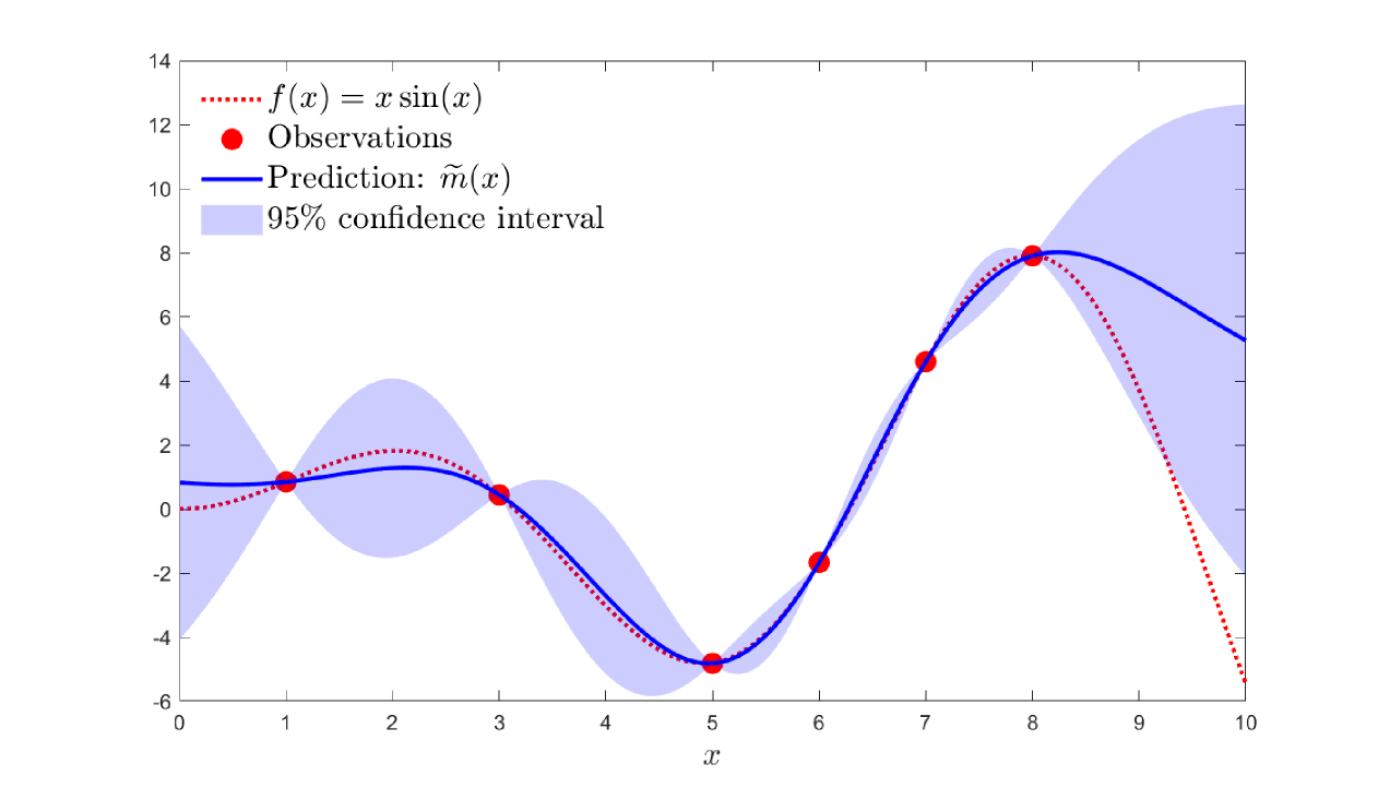
Figure 2: Illustration of Gaussian Process Regression. The dotted is the true function while the solid line is the posterior mean of the fitted GP. The shaded region plots the 95% confidence interval.

Figure˜2 illustrates a GPR in a one-dimensional setting in which the true function is $f(x)=x\sin(x)$. The example is for $N=5$ observations with observation noise $\sigma_{n}=0.01$. The true function is modeled as a GP with specification (19) and (20) for the mean and covariance kernel, respectively. The posterior mean is calculated according to equation (21) and is shown in the solid line. The shaded region plots the 95% confidence interval around the posterior mean and is computed based on the posterior variance (22).

3.2 Deep Kernel Gaussian Process

We use the Deep Kernel Gaussian Process (DKGP) proposed by Wilson, Hu, Salakhutdinov, and Xing (2016). A DKGP is a GP whose covariance kernel embeds a neural network component within a “standard” kernel as follows:

$$k_{\mbox{DK}}(\boldsymbol{x},\boldsymbol{x}^{\prime};\boldsymbol{\theta},\boldsymbol{w})=k\left(NN(\boldsymbol{x};\boldsymbol{w}),NN(\boldsymbol{x}^{\prime};\boldsymbol{w});\boldsymbol{\theta}\right)$$ (24)

where $NN(\cdot;\boldsymbol{w})$ is a neural network with hyperparameters $\boldsymbol{w}$, and $k(\cdot,\cdot;\boldsymbol{\theta})$ is a “regular” kernel such as the Matern 5/2 kernel (20). That is, a deep kernel (24) first uses a neural network $NN(\cdot;\boldsymbol{w})$ to process the input $\boldsymbol{x}$ before feeding the extracted feature(s) $NN(\boldsymbol{x};\boldsymbol{w})$ into a standard kernel $k(\cdot,\cdot;\boldsymbol{\theta})$.

To see why it is necessary to use a deep kernel in our setting, consider Figure˜3. Panel A illustrates a slice of the scaled value function $v(t,w,k,\mu_{P},s)$ along the liquid wealth share $w$ dimension (holding all other variables fixed). We see that the value function consists of two relatively flat regions, below $w=0.15$ and above $w=0.30$, with a sharp transition in the intermediate region between $w=0.15$ and $w=0.30$.

The sharp transition in the value function is a generic feature of our problem and is due to the possibility of default. The logic is as follows. Defaulting next period is likely when current liquidity $w$ is low; in this case, the current period’s value function primarily depends on the value of default $v_{D}(t+1,s^{\prime})$ next period which is low. Conversely, defaulting next period becomes unlikely when current liquidity $w$ is high and the current period’s value function primarily depends on the much larger non-default value next period $v(t+1,w^{\prime},k^{\prime},\mu_{P}^{\prime},s^{\prime})$. The sharp transition for intermediate liquidity $w$ captures the transition between defaulting and not defaulting next period.

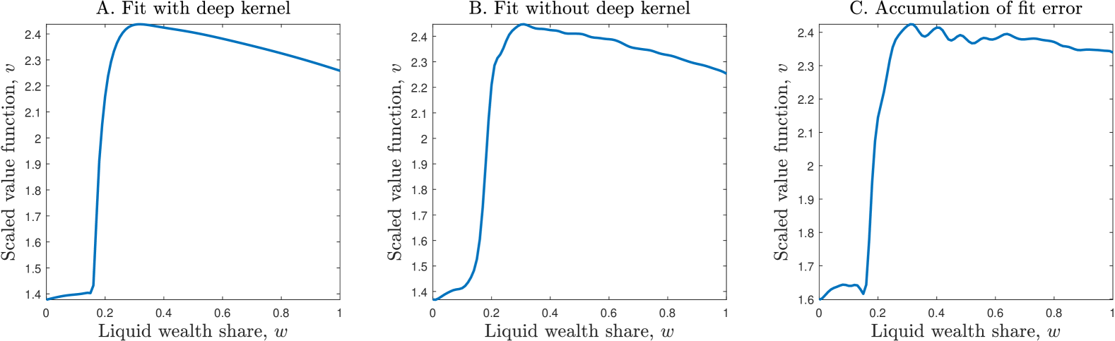
Figure 3: Illustration of necessity of Deep Kernel Gaussian Process. Panel A illustrates the value function when the model is solved using DKGP at every single step. Panel B illustrates the solution from a single backward induction step when the value function is fitted using a standard kernel. Panel C illustrates the accumulation of error over successive steps of backward induction when the value function is fitted using a standard kernel.

Sharp transitions are challenging for standard kernels to capture. The reason is that standard kernels such as the Matern kernel (20) feature a constant lengthscale along each dimension. In contrast, the value function in our setting features several lengthscales—long lengthscales are necessary to capture the slowly-varying value function when $w$ is low or high, while a short lengthscale is needed to capture the fast-varying value function for intermediate values of $w$. In addition, these lengthscales vary over the entire state space as both the location and speed of the sharp transition depend on all state variables.

Panels B and C of Figure˜3 illustrates the pitfalls of using a single lengthscale to fit a multi-lengthscale value function. Maximum likelihood estimation fits a short lengthscale to capture the sharp transition. The resulting fitted GP is fast-varying and contains wiggles (see panel B). These wiggles accumulate over successive steps of backward induction and ultimately results in a very noisy value function after sufficiently many steps (see panel C of Figure˜3).

The deep kernel (24) captures state-dependant lengthscales through its neural network component. This can be seen in Panel A of Figure˜3 which plots the fitted value function when a DKGP is used.

4 Quantitative Analysis

We begin by calibrating the model in Section˜4.1 and describing the model’s solution in Section˜4.2. We then report our model’s implications for optimal private asset allocation. Section˜4.3 and Section˜4.4 describe the optimal allocations over the LP’s life cycle and how business cycle conditions alter those allocations, respectively. Section˜4.5 shows that, for long-term PE investors, whether or not PE returns must first be “unsmoothed” prior to making inferences and allocation decisions may be a moot point. Section˜4.6 examines the impact of the risk weights on the LP’s portfolio allocation. Appendix C provides details on the numerical implementation of the model.

4.1 Calibration

We use the parameters listed in Table˜1. We calibrated the model at a quarterly frequency and take the investment horizon to be $T=40$ quarters or 10 years.

We take state $s=1$ to be a recessionary state and state $s=2$ to be an expansionary state. We set the transition probabilities for the macroeconomic state to $p_{12}=0.25$ and $p_{21}=0.05$ based on the duration of NBER recessions in the post-WWII sample. This implies recessions and expansions last for 4 and 20 quarters on average, respectively. In what follows, we use NBER recession dates when estimating parameter values that depend on the macroeconomic state.

Description	Symbol	Value
		$s=1$	$s=2$
Investment horizon, quarters	$T$	40
Macro transition probability	$p_{ss^{\prime}}$	0.25	0.05
PE call rate, new commitments	$\lambda_{N}(s)$	0.18	0.047
PE call rate, existing commitments	$\lambda_{K}(s)$	0.050	0.078
PE distribution rate	$\lambda_{D}(s)$	0.028	0.071
PE liquidation discount	$\alpha(s)$	0.66	0.90
Risk-free rate	$\log R_{f}(s)$	0.0028	0.0051
Stock expected return	$\mu_{S}(s)$	0.0079	0.0238
Stock return volatility	$\sigma_{S}(s)$	0.1493	0.0829
Stock-PE return correlation	$\rho(s)$	0.9527	0.4575
PE return volatility	$\sigma_{P}(s)$	0.0768	0.0424
PE expected return autocorrelation	$\varrho_{P,1}+\varrho_{P,2}$	0.201
PE expected return state-dependance	$\nu_{P}(s)$	0.0024	0.0317
Risk aversion	$\gamma$	2
PE adjustment costs	$\gamma_{N}$	0.1
PE adjustment costs	$\overline{n}$	0
Stock adjustment costs	$\gamma_{S}$	0.01
Risk budget threshold	$\overline{\theta}$	1
Risk budget cost	$\kappa$	1
Risk weight, bonds	$\theta_{B}$	0
Risk weight, stocks	$\theta_{S}$	1.5
Risk weight, PE	$\theta_{P}$	1.5

Table 1: Parameters. We simulate the model at a quarterly frequency using the parameters in this table.

We use quarterly data provided by Liberty Mutual Investments (LMI) on its PE holdings to calibrate various PE-related parameters. This data contains LMI’s total PE exposure broken down by asset class—buyout, growth, and venture capital. For each asset class, the data details total exposure over time ($K_{t}+P_{t}$ in the model) and breaks this exposure down into outstanding commitments ($K_{t}$) and the NAV of current PE investments ($P_{t}$). The data also include information on LMI’s contributions, distributions received from its PE investments, and the number of investees LMI invests in. In estimating parameters, we restrict attention to buyout funds from the moment when the number of buyout investees first reach 10. The resulting sample starts in 1996Q4 and ends in 2023Q4; all estimates are based on this sample period.

$\mbox{Contribution}_{t}$ in the LMI data corresponds to $\lambda_{K}(s_{t})K_{t-1}+\lambda_{N}(s_{t})N_{t-1}$ in the model. We estimate the call rates using the following regression:

$$\frac{\mbox{Contribution}_{t}}{K_{t-1}}=a(s_{t})+b(s_{t})\frac{N_{t-1}}{K_{t-1}}+\epsilon_{t},$$ (25)

where the constant $a(s_{t})$ maps to $\lambda_{K}(s_{t})$ and the slope coefficient $b(s_{t})$ maps $\lambda_{N}(s_{t})$. We estimate regression (25) separately for recessionary ($s=1$) and expansionary ($s=2$) regimes to obtain state-dependant estimates for the call rates. The resulting point estimates give $\lambda_{K}(1)=0.050$ and $\lambda_{N}(1)=0.18$ during recessions, and $\lambda_{K}(2)=0.078$ and $\lambda_{N}(2)=0.047$ during expansions.

We set the PE payout rate $\lambda_{D}(s)$ to be the average payout rate in the LMI dataset. This results in $\lambda_{D}(1)=0.028$ and $\lambda_{D}(2)=0.071$ during recessions and expansions, respectively.

We calibrate the discount from liquidating PE investments $\alpha(s)$ based on estimates of transaction costs in the secondary market for selling PE stakes from Nadauld, Sensoy, Vorkink, and Weisbach (2019, Table 1). They find that the purchase price, expressed as a pecent of NAV, is 86% on average and drops to 66% during 2008-09 (the only recession in their sample). We set $\alpha(1)=0.66$ and $\alpha(2)=0.90$ during recessions and expansions, respectively, based on these estimates.

We calibrate the returns processes as follows. We take the series for the risk-free rate and aggregate stock returns from Kenneth French’s website. We set the risk-free rate and expected stock returns to their sample averages during recessions and expansions; this results in $\log R_{f}(1)=0.0028$ and $\log R_{f}(2)=0.0051$ for the risk-free rate and $\mu_{S}(1)=0.0079$ and $\mu_{S}(2)=0.0238$ for expected stock returns.

LMI data includes quarterly mark-to-market information for the NAV of its PE investments; this allows us to compute the realized PE return $R_{P,t}$ as the ratio of the mark-to-market and the lagged NAV value. We use moments of the resulting time series for $R_{P,t}$ to estimate the PE return process. We set the stock-PE return correlation $\rho(s)$ to its sample correlation; this results in $\rho(1)=0.9527$ and $\rho(2)=0.4575$ during recessions and expansions, respectively. We restrict $\varrho_{P,1}=\varrho_{P,2}$ and choose the remaining parameters of the PE expected return process (13) and PE return volatility $\sigma_{P}(s)$ by matching the following data moments: (1) a PE expected return $\mathbb{E}\left[\log R_{P,t+1}|s_{t}\right]$ of 0.0052 and 0.0392 during recessions and expansions, respectively, (2) a PE return volatility $\sigma\left(\log R_{P,t+1}|s_{t}\right)$ of 0.0772 and 0.0427 during recessions and expansions, respectively, and (3) a PE return autocorrelation of $\rho\left(R_{P,t},R_{P,t+1}\right)=0.1425$. This results in $\varrho_{P,1}=\varrho_{P,2}=0.1006$, $\nu_{P}(1)=0.0024$ and $\sigma_{P}(1)=0.0768$ during recessions, and $\nu_{P}(2)=0.0317$ and $\sigma_{P}(2)=0.0424$ during expansions.

We set the risk weights for stocks and private equity to $\theta_{S}=1.5$ and $\theta_{P}=1.5$, respectively. Since the overall risk budget $\overline{\theta}$ is normalized to 1, these risk weights imply a 50% risk charge for stocks and private equity. These values are in line with equity risk charges used by ratings agencies for assessing insurers’ RBC adequency (see S&P Global 2023, Table 14). The risk weight for risk-free bonds is $\theta_{B}=0$. We set the cost parameter for the proportional risk cost (6) to $\kappa=1$.

We set risk aversion to $\gamma=2$ which is standard. The remaining parameters relate to adjustment costs. We set $\gamma_{N}=0.1$ and $\overline{n}$ for PE adjustment costs, and $\gamma_{S}=0.01$ for stock adjustment costs.

4.2 Value and policy functions

We begin by illustrating the solution for the scaled value function and the policy functions; recall that the scaled and unscaled value functions are related through equations (17) and (18).

Value functions.

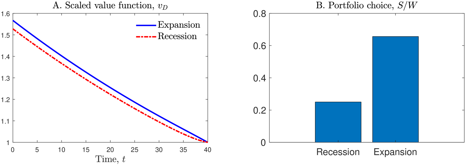
Figure 4: Solution after defaulting. Panel A plots the scaled value function after defaulting $v_{D}(t,s)$; it is related to the unscaled value function through equation (17). Panel B plots the optimal allocation to stocks after defaulting.

Figure˜4 plots the solution after defaulting. Panel A plots the scaled value function $v_{D}(t,s)$. The value function is declining over time since the investment horizon over which to accumulate wealth shrinks over time. The value function is also higher during expansions than recessions. Panel B plots the portfolio choice after defaulting. The investor’s allocation depends only on the macroeconomic state and does not vary over time—the optimal allocation to stocks is 25% and 66% during recessions and expansions, respectively; all remaining wealth are allocated to bonds.

Next, we illustrate the solution before defaulting during which the scaled value function $v(t,w,k,\mu_{P},s)$ depends on time $t$, the liquid fraction of total wealth $w=W/(W+P)$, uncalled commitments relative to total wealth $k=K/(W+P)$, the expected return for PE $\mu_{P}$, and the macroeconomic state $s$.

Figure˜5 plots the distribution of the expected PE return $\mu_{P}$. Panel A plots the unconditional distribution while panel B plots the conditional distribution given the macroeconomic state. Expected returns for PE are higher during expansions under our baseline calibration with expected returns averaging $\mathbb{E}[\mu_{P,t}|s_{t}=1]=0.0052$ and $\mathbb{E}[\mu_{P,t}|s_{t}=2]=0.0392$ per quarter during recessions and expansions, respectively. From panel B, we also see that the distribution of expected PE returns is wider during expansions than recessions; this is on account of higher PE return volatilities during recessions.

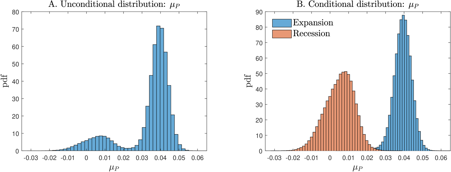
Figure 5: Distribution for $\mu_{P}$. Panel A plots the stationary distribution for $\mu_{P}$ whose law of motion is given by equation (13). Panel B plots the distribution for $\mu_{P}$ conditional on the current macroeconomic state.

Figure˜6(a) illustrates the scaled value function $v(t,w,k,\mu_{P},s)$ at $t=0$. Panel A plots the value function in the expansionary state ($s=2$) when the expected return on PE is equal to its mean conditional on $s=2$. We see that the value function $v$ is a non-monotonic function of the liquid fraction of total wealth $w$. Specifically, $v$ is first increasing in $w$ when $w$ is sufficiently small (e.g., for $w<0.30$ when $k=0$) and then decreasing in $w$ when $w$ is sufficiently large (e.g., for $w>0.30$ when $k=0$).

The reason for this non-monotonicty is as follows. Defaulting becomes likely when $w$ is small; this is illustrated in Figure˜7 which plots the one quarter ahead default probabilities at $t=0$. When the current period’s liquid wealth is low, the LP becomes less likely to have enough liquid wealth next period to meet its capital commitments and to pay its risk budget cost (see equation (9)). Hence, the value function becomes increasing in $w$ when $w$ is small, as having more liquidity helps the LP avoid default. Instead, when $w$ is sufficiently large so that there is no risk of default, the LP’s value function becomes decreasing in $w$ because the LP would be able to achieve better investment outcomes had it allocated more of its wealth to PE.

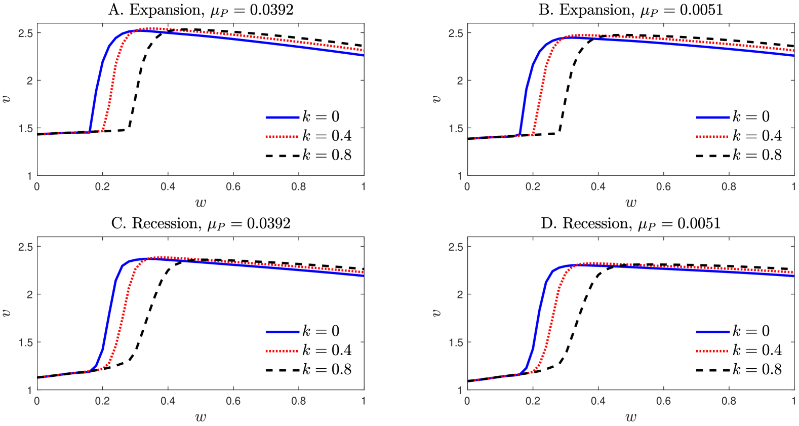
(a) Slices of the value function along the $w$ dimension.

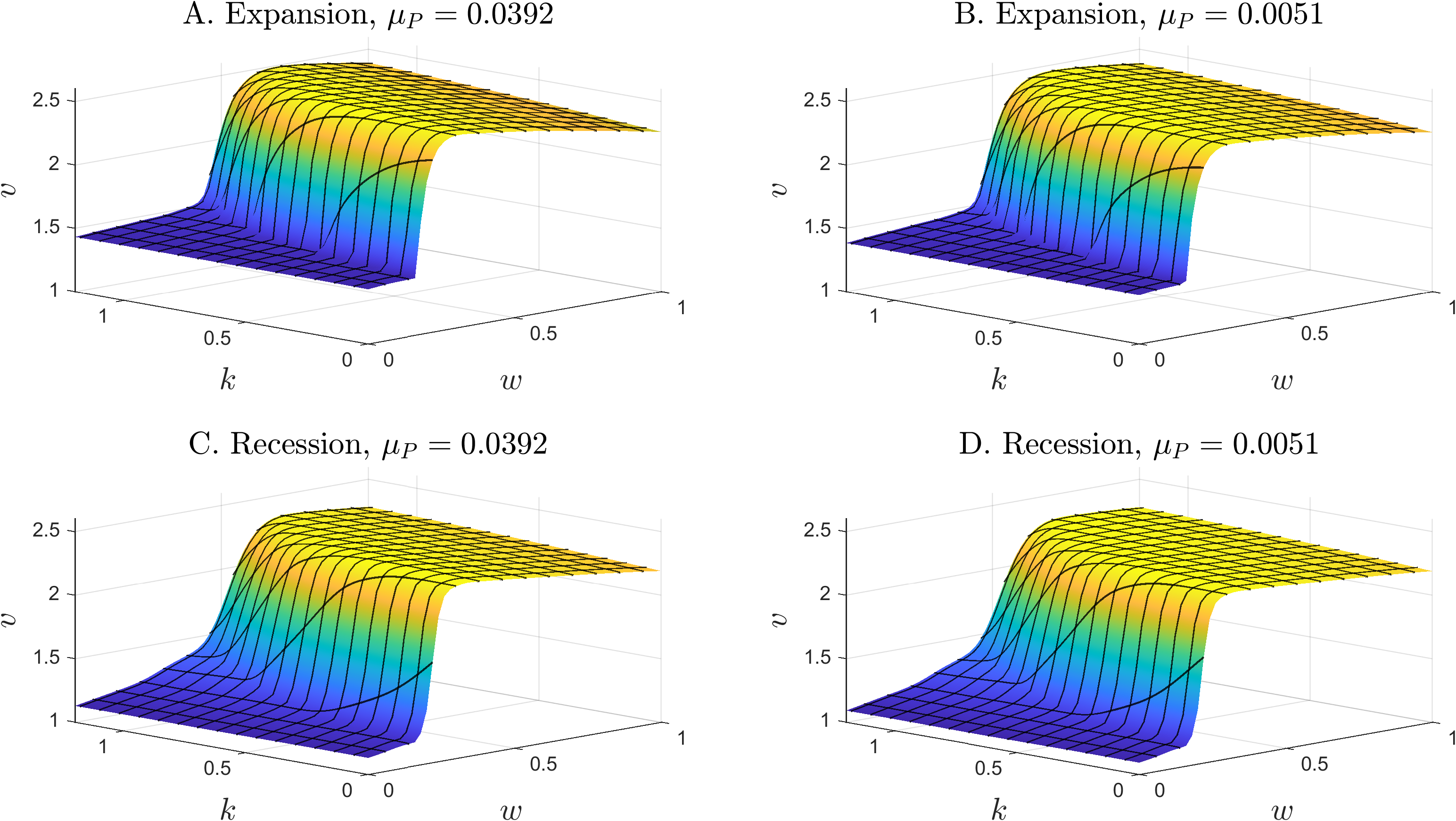
(b) Surface plots of the value function

Figure 6: Scaled value function at $t=0$. This figure illustrates the scaled value function before default $v(t,w,k,\mu_{P},s)$ at $t=0$. In both subfigures, the first (second) row displays the value function in the expansionary (recessionary) state. The first (second) column sets $\mu_{P}$ to its mean conditional on the expansionary (recessionary) state.

Figure 7: One quarter ahead default probabilites at $t=0$. This figure illustrates the one period ahead default probability at $t=0$. The first (second) row displays the default probabilities in the expansionary (recessionary) state. The first (second) column sets $\mu_{P}$ to its mean conditional on the expansionary (recessionary) state.

Similarly, the value function $v$ is non-monotonic in uncalled commitments relative to total wealth $k$. For example, in panel A of Figure˜6(a) we see that $v$ is decreasing in $k$ for small $w$ (e.g., when $w=0.2$) while $v$ is increasing in $k$ for large $w$ (e.g., when $w=0.8$). The reason is as follows. When the LP has little liquidity, default concerns become first order and having more uncalled commitments increases the likelihood of default, thereby decreasing $v$. In contrast, when the LP has sufficient liquidity and default is no longer a concern, higher uncalled commitments $k$ increases the LP’s PE exposure which increases $v$. This is because the presence of adjustment costs means that it takes time for the LP to build up its PE exposure through capital commitments.

Panel B of Figure˜6(a) plots the value function in the expansionary state when the PE expected return is low while panels C and D illustrate the value function in the recessionary state. The value function is monotonically increasing in the PE expected return $\mu_{P}$, as higher expected PE returns unambiguously translate into higher expected utility. Moreover, the value function is lower during recessions (panels C and D) compared to expansions (panels A and B), reflecting the less favorable investment opportunities during economic downturns. Despite these level differences, we see that the shape of the value function remains similar across different macroeconomic states and PE expected returns. Figure˜6(b) illustrates further details of the value function using three-dimensional surface plots.

New commitments.

Figure˜8 illustrate the optimal policy for new PE commitments, scaled with respect to total wealth, at $t=0$. We see that new PE commitments are increasing in the liquid fraction of total wealth $w$ and decreasing in the uncalled commitments relative to total wealth $k$. The LP becomes less willing to commit new capital to PE when default concerns are high as defaulting leads to costly PE liquidations. This is why new PE commitments are low when $w$ is low or $k$ is high. Instead, when default is unlikely, the LP commits more capital to PE in order to increase its PE exposure and thereby lower its future liquid wealth share (as discussed above, the value function becomes decreasing in $w$ in the absence of default concerns).

Figure 8: New commitments at $t=0$. This figure illustrates new commitments relative to total wealth, $N/(W+P)$, at $t=0$. The first (second) row displays the results for the expansionary (recessionary) state. The first (second) column sets $\mu_{P}$ to its mean conditional on the expansionary (recessionary) state.

Comparing panels A and B of Figure˜8, and panels C and D of Figure˜8, we see that current PE expected returns $\mu_{P}$ have surprisingly little impact on new commitments across both expansionary and recessionary states. This muted response stems from the inherent delay between making commitments and their eventual conversion into PE investments. Because PE expected returns exhibit low quarterly autocorrelation in the baseline calibration ($\varrho_{P}=0.20$), initial differences in $\mu_{P}$ largely dissipate before committed capital is called. Consequently, optimal commitment levels depend primarily on the expected conditional return $\mathbb{E}[\mu_{P,t}|s_{t}]$ rather than the current level of $\mu_{P}$, since only invested capital (NAV) ultimately generates PE returns.

Finally, comparing across macroeconomic states, we see from Figure˜8 that new commitments are higher during expansions than recessions. Figure˜1(a) in Appendix C uses three-dimensional surface plots to illustrate further details regarding new commitments.

Allocation to stocks.

Figure 9: Allocation to stocks at $t=0$. This figure illustrates the optimal allocation to public stocks, expressed as a fraction of total wealth, at $t=0$. The first (second) row displays the optimal allocation in the expansionary (recessionary) state. The first (second) column sets $\mu_{P}$ to its mean conditional on the expansionary (recessionary) state.

Figure˜9 illustrates the optimal allocation to public stocks as a fraction of total wealth at $t=0$ (see Figure˜1(b) in Appendix C for surface plots that display further details). Panel A depicts this allocation during the expansionary state, with PE expected returns at their mean conditional on $s=2$. When liquid wealth $w$ exceeds 0.3, making default risk negligible, two patterns emerge. First, stock allocation increases with $w$, reflecting a rebalancing mechanism: as liquid wealth rises and PE exposure ($1-w$) mechanically falls, the LP maintains its desired risk exposure by increasing its allocation to public stocks. For example, the portfolio shifts from 50% PE, 17% stocks, and 33% bonds at $w=0.5$ to 20% PE, 46% stocks, and 34% bonds at $w=0.8$. Second, stock allocation remains independent of uncalled commitments $k$. This is because, absent default risk, the value function depends primarily on next period’s total wealth growth rate. Since uncalled commitments affect total wealth only after their conversion to PE investments (NAV), which occurs with a lag, they have no immediate impact on portfolio growth (see equation (B.9)) and therefore do not interact with the allocation decision for public stocks.

When default risk is non-negligible, a different mechanism is at play. For example, default occurs with certainty when $w=0.1$ for the levels of $k$ considered here (see Figure˜7). In this case, the LP makes its stock allocation decision knowing that it will default on its PE commitments and incur a PE liquidation loss next period. The LP chooses to maximize its stock allocation to compensate for this loss when macroeconomic conditions are favorable (see panels A and B of Figure˜9). Conversely, it takes a conservative approach and does not allocate anything to public stocks when macroeconomic conditions are unfavorable (see panels C and D of Figure˜9).

However, this default mechanism is rarely at work along the optimal path when we simulate the model. The LP tries to avoid default since defaulting is costly. The cumulative default rate over the LP’s 10 year investment horizon is only 0.1%.

4.2.1 Marginal value of liquidity

The illiquid nature of PE assets makes liquidity management central. Indeed, the LP must finance its capital calls out of its liquid wealth or suffer the consequences of default. The marginal value of liquidity at time $t$, measured in units of certainty equivalent terminal wealth, is given by

$$\frac{\partial}{\partial W}(W+P)v(t,w,k,\mu_{P},s)=v+(1-w)v_{w}-kv_{k}.$$ (26)

On the left-hand side of equation (26), $(W+P)v(t,w,k,\mu_{P},s)$ expresses the value function $V(t,w,k,\mu_{P},s)$ in certainty equivalent units of terminal wealth (see equation (18)). Here, $W+P$ is current total wealth and $v(t,w,k,\mu_{P},s)$ is the certainty equivalent value per unit of wealth. On the right-hand side, the $v$ term captures the direct effect of an additional unit of wealth. The $(1-w)v_{w}$ and $-kv_{k}$ account for compositional effects due to changes in the liquid fraction of wealth $w$ and uncalled commitments relative to total wealth $k$. The formulation of the marginal value of liquidity (26) is analogous to the marginal value of cash in the liquidity management model of Bolton, Chen, and Wang (2011, 2013).

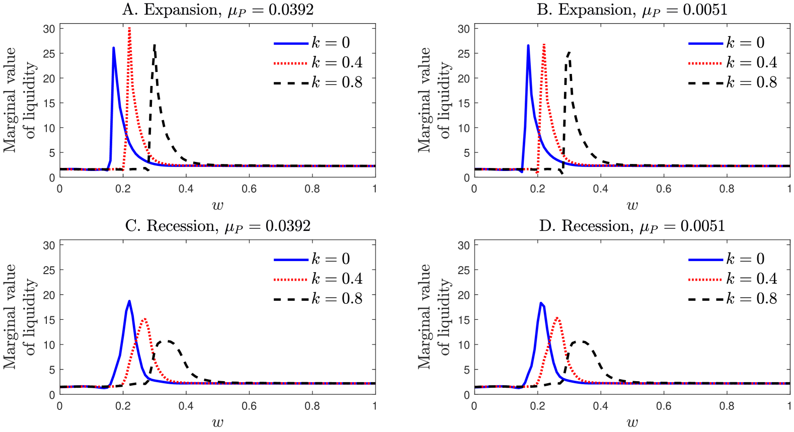
(a) Slices of the marginal value of liquid wealth along the $w$ dimension.

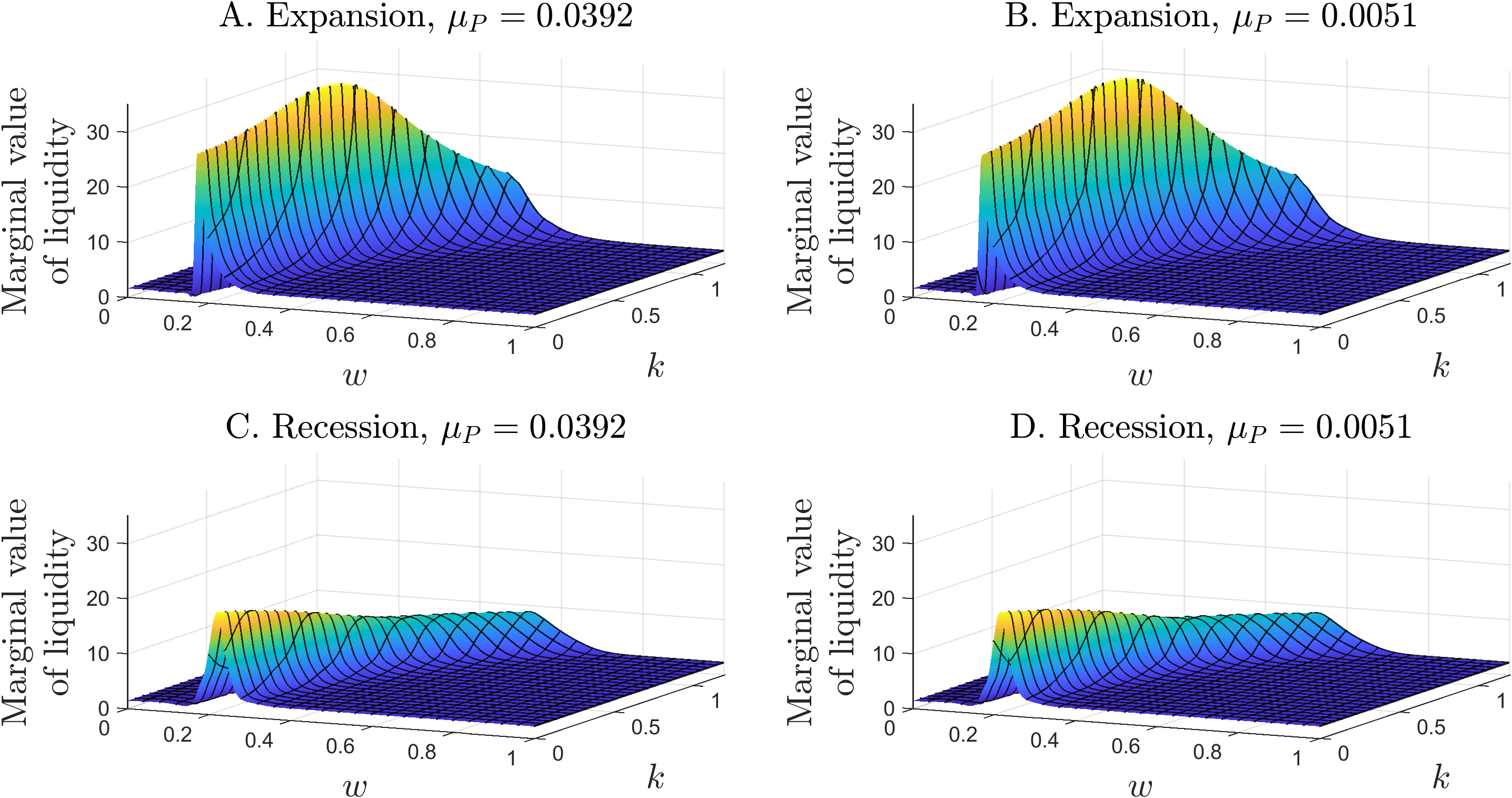
(b) Surface plots of the marginal value of liquid wealth

Figure 10: Marginal value of liquid wealth at $t=0$. This figure illustrates the marginal value of liquid wealth (26) at $t=0$. In both Figure˜10(a) and Figure˜10(b), the first (second) row displays the value function in the expansionary (recessionary) state; the first (second) column sets $\mu_{P}$ to its mean conditional on the expansionary (recessionary) state.

Figure˜10(a) illustrates the marginal value of liquid wealth (26) at $t=0$; Figure˜10(b) uses surface plots to provide additional details. We see that the marginal value of liquid wealth is highly sensitive to default risk. As the liquid fraction of wealth $w$ decreases, default probabilities increase (see Figure˜7), leading to a spike in the marginal value of liquidity.

For instance, panel A of Figure˜10(a) shows that when $k=0.4$, the macroeconomic state is expansionary, and $\mu_{P}$ equals its conditional mean in the expansionary state, the marginal value of liquidity equals 2.28 when $w=1$ and default is not a concern. However, as $w$ drops to $0.22$, the marginal value of liquidity rises to 30.21; at this point, the one-quarter-ahead default probability is 0.21 and rapidly approaches 1 as $w$ declines further. Eventually, as $w$ continues to decrease, the marginal value of liquidity levels off because default becomes inevitable, so that marginal increases in liquid wealth no longer helps to avert default. When $w=0$ and default is certain, the marginal value of liquidity falls to 1.62—this lower certainty equivalent value reflects the lower growth rate of wealth after the LP defaults and loses access to PE investing.

The plots further demonstrate how the marginal value of liquidity varies over the state space. For example, the location of the peak in the marginal value of liquidity depends strongly on the ratio of uncalled capital to wealth $k$; higher values of $k$ result in the peak occurring at larger values of $w$.

4.3 Life cycle dynamics

We now turn to the life cycle dynamics of the LP’s portfolio. We assume that the LP starts out at $t=0$ without any PE investments (i.e., $P_{0}=K_{0}=0$) and a units of liquid wealth $W_{0}=1$ so that $k_{0}=0$ and $w_{0}=1$. The initial macroeconomic state $s_{0}$ and PE expected return $\mu_{P,0}$ are drawn from their stationary distributions. We then simulate the LP’s portfolio allocation over its investment horizon of 10 years. Figure˜11 shows the outcome—the solid line plots the average outcome at each point in time while the shaded region plots the 95% confidence interval around the average.

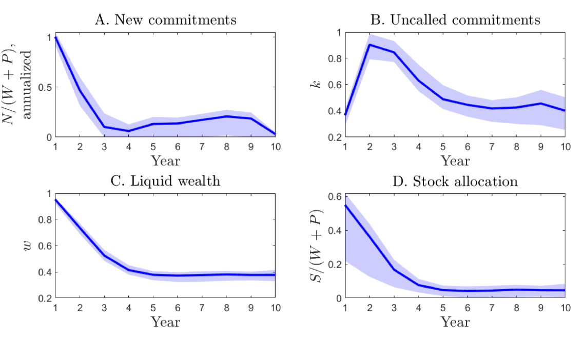
Figure 11: Life cycle dynamics. This figure illustrates the life cycle dynamics of the LP’s portfolio. The solid line plots the average outcome in each year while the shaded region provides the 95% confidence interval. Panels A through D plot the outcomes for new commitments, uncalled commitments, liquid wealth, and the stock allocation, respectively. All outcomes are shown relative to total wealth.

Starting out, the LP aggressively makes new capital commitments in the first two years to rapidly increase its PE exposure (see panel A of Figure˜11). For example, new commitments average 100% of total wealth during the first year before dropping to 47% and 10% of total wealth on average in the second and third years, respectively. As a result, uncalled capital increases and peaks at an average of 90% and 85% of total wealth during the second and third years (see panel B). This is accompanied by a drop in the liquid portion of wealth (see panel C) or, equivalently, an increase in the LP’s PE exposure. Specifically, the LP’s NAV in PE investments rises to 26% and 47% of total wealth on average in the second and third years, respectively, before reaching 62% of total wealth by year 5. From year 5 onwards, the LP is in maintenance mode, making new commitments to maintain its PE exposure at an average of 62% of total wealth until the investment horizon is reached at year 10.

Stock allocation initially starts high (see panel D); for example, stock allocation averages 55% of total wealth in the first year. This is because the LP can only achieve its target aggregate risk exposure through public stocks before its PE exposure is built up. The wide confidence interval for stock allocation during this initial phase is due to differences in stock allocation across the business cycle which we discuss in Section˜4.4. The stock allocation subsequently drops to 5% of total wealth on average during the LP’s maintenance phase.

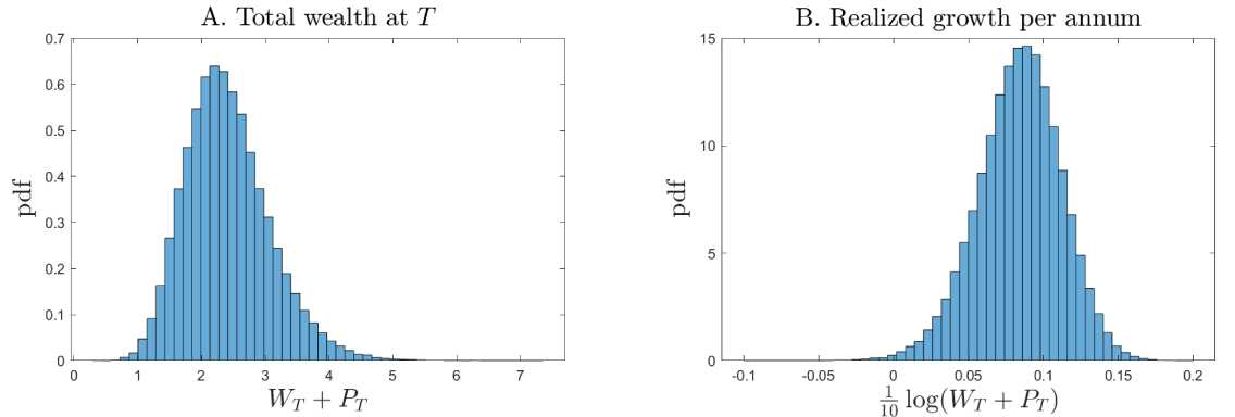
Figure 12: Total wealth outcome distribution. This figure illustrates the distribution of total wealth outcomes at the end of the investment horizon $t=T$. The initial total wealth is $W_{0}+P_{0}=1$. Panel A plots the distribution for total wealth $W_{T}+P_{T}$. Panel B plots the distribution for the realized growth in total wealth per annum, $\log(W_{T}+P_{T})/10$.

Figure˜12 shows the distribution of outcomes at the terminal date $T$. Panel A plots the distribution of for total wealth $W_{T}+P_{T}$. Starting from a unit initial total wealth, the LP’s terminal wealth equals 2.41 on average with a standard deviation of 0.66. This wealth distribution translates into a certainty equivalent wealth of $\mathbb{E}[v(t=0,w_{0},k_{0},\mu_{P},s)\left|w_{0}=1,k_{0}=0\right.]=2.25$ on the initial date. Panel B illustrates the distribution of final outcomes in terms of the annualized realized total returns $\frac{1}{10}\log((W_{T}+P_{T})/(W_{0}+P_{0}))$. The annualized realized total return over the LP’s investment horizon has a mean of 8.41% and a standard deviation of 2.78%. Note that this seemingly low standard deviation is because we are reporting the standard deviation of annualized long-horizon returns (see Footnote˜5).

4.3.1 Heuristic versus dynamic private asset allocation

In practice, investors often use heuristics to simplify private asset allocation decisions. One common heuristic is to split the allocation problem into two steps. In the first step, investors determine a long-run target portfolio by solving a static portfolio choice problem that abstracts from liquidity risk and the timing lags inherent in PE investing (e.g., a traditional Markowitz approach). In the second step, they adjust their allocations to reach the targets from the first step by accounting for the delays between capital commitments, capital calls, and eventual distributions (see, for example, Takahashi and Alexander 2002). We demonstrate that portfolio allocations derived from our dynamic model can differ dramatically from these heuristic approaches. Specifically, we show that portfolio outcomes from our dynamic model, starting from year 5 when the LP has reached the maintenance phase, substantially differ from the long-run target portfolio obtained under the heuristic approach. We provide details below.

Within our framework, the first step of the heuristic approach corresponds to solving

$$V_{\mbox{heuristic}}(t,W_{total},s)=\max_{S,B,P\geq 0}\mathbb{E}\left[V_{\mbox{heuristic}}(t+1,W^{\prime}_{total},s^{\prime})\left|W_{total},s\right.\right]$$ (27)

subject to

$$W^{\prime}_{total} =R_{P}^{\prime}PR_{S}^{\prime}S+R_{f}(s)B-W_{total}\Gamma(\theta),$$

$$\theta =\frac{\theta_{B}B+\theta_{S}S+\theta_{P}P}{B+S+P},$$

$$W_{total} =S+B+P,$$

and the terminal condition $V_{\mbox{heuristic}}(T,W,s)=W^{1-\gamma}/(1-\gamma).$ The heuristic problem (27) resembles the full problem (16) but reduces the total number of state variables by abstracting away from the illiquidity of PE investments. In implementing the heuristic problem (27), we further set $\mu_{P}=\mathbb{E}[\mu_{P,t}|s_{t}=s]$ to its mean conditional on the macroeconomic state. In Appendix B, we show that the solution to the heuristic problem (27) amounts to optimizing the certainty-equivalent growth rate of total wealth at each point in time. The solution is static in the sense that the optimal portfolio weights depend solely on the macroeconomic state $s$ and do not otherwise change over time.

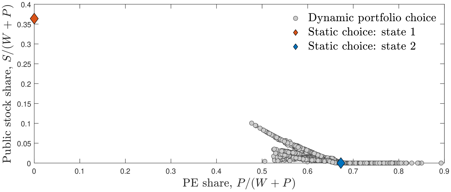
Figure 13: Portfolio choice: heuristic vs. dynamic private asset allocation. This figure compares the portfolio outcomes under the heuristic problem (27) (shown by the diamonds) against the outcomes under the full dynamic allocation problem (16) (shown in the circles). Outcomes for the latter correspond are from year 5 onwards during which the maintenance phase has been reached.

Figure˜13 compares the portfolio outcomes under the heuristic approach (27) with those under our full dynamic model (16). The circles represent the portfolio allocations derived from our dynamic model for year 5 onwards—when the limited partner (LP) has entered its maintenance phase—while the diamonds show the static portfolio choices obtained from solving (27) for each macroeconomic state.

Under our baseline calibration (Table˜1), the heuristic approach yields an optimal portfolio allocation of 67.3% in private equity (PE) and 0% in stocks (with the remainder in bonds) in the expansionary state, and 0% in PE and 36.4% in stocks in the recessionary state. In contrast, the optimal dynamic allocation maintains a PE allocation of at least 45% during the maintenance phase, while the stock allocation does not exceed 10%. This difference in outcomes is especially stark during the recessionary state, where the heuristic outcome falls entirely outside the range of values generated by the optimal dynamic allocation.

4.4 Business cycle dynamics

Figure˜14 illustrates how business cycle conditions affect the life cycle dynamics of the LP’s portfolio. The solid and dashed lines plot the average outcomes conditional on the macroeconomic state being in a expansion and a recession, respectively; the shaded 95% confidence intervals are also conditional on the macroeconomic state. Overall, we see that the allocation patterns across the business cycle are similar compared to the unconditional case discussed in Section˜4.3.

The most notable difference across the business cycle is the difference in the LP’s stock allocation, particularly during the ramping-up phase (see panel D of Figure˜14). For instance, in year 1, stock allocations average 62% of total wealth during expansions compared to 38% during recessions. This difference narrows to about 2% of total wealth by the maintenance phase from year 5 onwards.

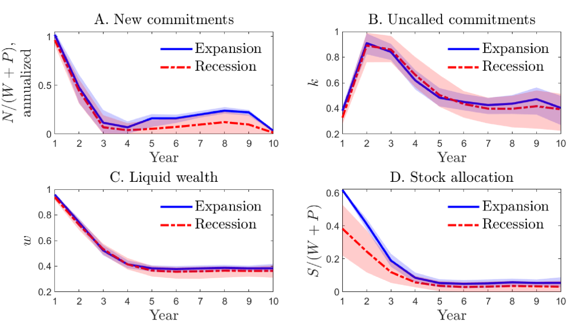
Figure 14: Life cycle dynamics over the business cycle. This figure illustrates the life cycle dynamics of the LP’s portfolio after conditioning on business cycle conditions. Panels A through D plot the outcomes for newcommitments, uncalled commitments, liquid wealth, and the stock allocation, respectively, where all outcomes are shown relative to total wealth. The solid (dashed) line shows the average outcome conditional on a expansionary (recessionary) state. Shaded regions indicated 95% confidence intervals, conditional on the macroeconomic state.

There is a smaller difference in new commitments across the business cycle (see panel A). For example, During the ramping-up phase in the first three years, new commitments are lower during recessions compared to expansions by about 5% of total wealth on average. Similarly, panels B and C show that the difference in uncalled commitments and liquid wealth over the business cycle is smaller on average compared to the differences in stock allocation. For example, the difference in PE allocation across the business cycle averages 2% of total wealth over the lifetime of the fund.

The main reason for the pronounced difference in stock allocation across the business cycle, as opposed to PE allocation, is due to adjustment costs. PE allocation involves significant adjustment costs, whereas adjustment costs for stocks are negligible. Therefore, the LP keeps the PE allocation relatively stable across the business cycle and primarily adjusts its exposure to aggregate risks through stock allocation.

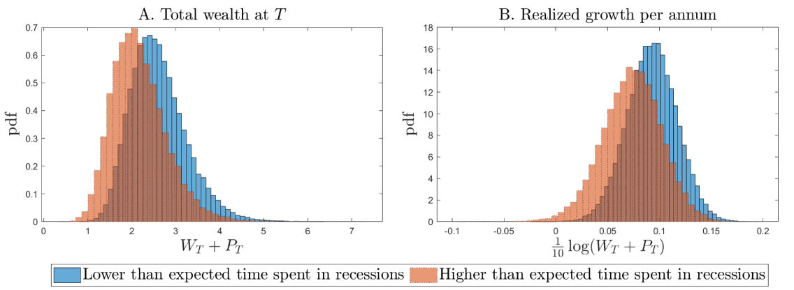
Figure 15: Business cycles and total wealth outcomes. This figure illustrates the distribution of total wealth outcomes at the end of the investment horizon $t=T$. The initial total wealth is $W_{0}+P_{0}=1$. Panel A plots the distribution for total wealth $W_{T}+P_{T}$. Panel B plots the distribution for the realized growth in total wealth per annum, $\log(W_{T}+P_{T})/10$. The solid (dashed) bars plot the outcomes conditional on the LP experiencing a lower (higher) than expected number of recessions over its investment horizon.

Figure˜15 plots the distribution of outcomes at the terminal date $T$ conditional on business cycle conditions encountered over the LP’s investment horizon. The transition probabilities for the macroeconomic state from Table˜1 imply that recessions occur 1/6 of the time. The solid blue (dashed red) bars plot outcome distributions conditional on the LP encountering recessions for less (more) than 1/6 of the time over its investment horizon. Panel A plots the outcomes for wealth. On average, the LP ends up with a terminal wealth of 2.60 and 2.17 conditional on experiencing a lower- and higher-than expected number of recessions, respectively. The corresponding standard deviations of terminal wealth are similar: 0.63 and 0.61 conditional on experiencing a lower- and higher-than expected number of recessions, respectively. The outcomes in terms of annualized realized total returns are shown in panel B. Conditional on experiencing a lower than expected number of recessions, the realized annualized returns average 9.29% with a standard deviation of 2.40%. The annualized return averages 7.35% with a standard deviation of 2.83% if a higher than expected number of recessions is encountered instead.

4.4.1 Cost of ignoring business cycle when making PE allocations

Next, we illustrate the importance of accounting for business cycle conditions through the following exercise. We consider a naive LP whose decisions are based on a model that ignores business cycles. Specifically, this naive LP solves the model under the assumption that the economy is always in an expansionary state (i.e., this LP sets $s_{0}=2$, $p_{21}=0$, and uses the remaining parameters from Table˜1). The naive LP then applies the resulting policy functions, which ignore business cycle fluctuations, in a setting where such fluctuations are present. We compare the life cycle dynamics of this naive LP to the baseline case, where the LP optimally accounts for business cycle conditions. The results are shown in Figure˜16.

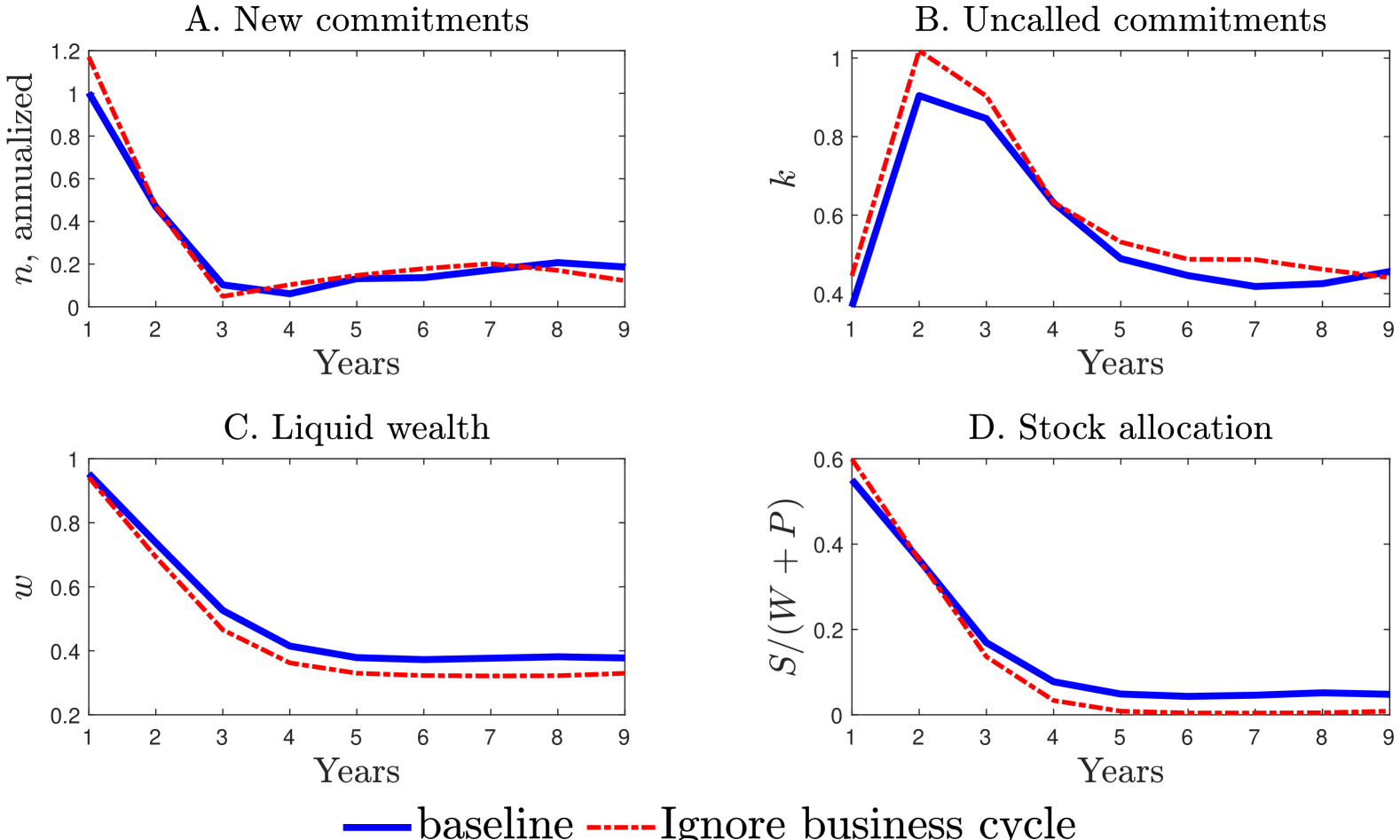
Figure 16: Life cycle outcomes without accounting for business cycles. The solid and dashed lines plot the average outcomes when business cycles are accounted for and not accounted for, respectively.

We observe that without considering the possibility of recessions, the LP’s PE allocation is significantly more aggressive compared to the optimal policy that accounts for business cycle fluctuations. For instance, in year 1, new commitments average 117% of total wealth compared to 100% in the baseline case. During the maintenance phase, the PE allocation averages 67% of total wealth, as opposed to 62% in the baseline case. Consequently, the naive LP defaults substantially more frequently—the naive LP’s 10-year cumulative default probability is 13.6% compared to only 0.1% under the optimal policy.

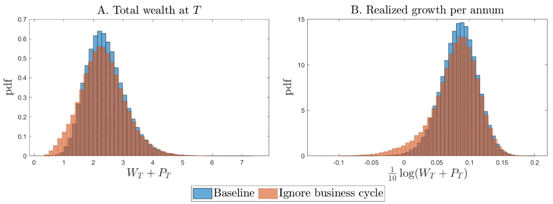
Figure 17: Total wealth outcome without accounting for business cycles. This figure illustrates the distribution of total wealth outcomes at the end of the investment horizon $t=T$. The initial total wealth is $W_{0}+P_{0}=1$. Panel A plots the distribution for total wealth $W_{T}+P_{T}$. Panel B plots the distribution for the realized growth in total wealth per annum, $\log(W_{T}+P_{T})/10$. The solid and dashed bars plot the outcomes for the baseline and a naive investor that ignores business cycles, respectively.

This large increase in default frequency has a significant negative impact on the naive LP’s final portfolio outcomes. Figure˜17 compares the outcome distributions for the naive investor against the baseline; panels A and B compare outcomes for terminal total wealth and annualized realized returns, respectively. Compared to the baseline investor that takes business cycles into account, the wealth total wealth distribution for the naive LP has a lower mean (2.32 vs. 2.41) and a higher volatility (0.75 vs 0.66). Similarly, the naive LP’s annualized realized returns have a lower mean (7.83% vs 8.41%) and a higher volatility (3.58% vs 2.78%). The biggest difference in outcomes, however, is heavier left-tail encountered by the naive investor. For example, the first and fifth percentiles for the naive LP’s realized annualized returns equal -3.06% and 1.14%, as opposed to 1.34% and 3.68% for the baseline case. The naive LP’s suboptimal policies translate into a 9.3% loss in initial total wealth—the naive LP’s certainty equivalent value is 2.04 compared to 2.25 for the baseline case.

These results underscore the importance of considering business cycle conditions when making optimal PE allocation decisions.

4.5 Does serial correlation in PE returns matter for long-term investors?

Positive serial correlation is a hallmark feature of the observed returns of illiquid alternative asset, PE investments included. A large literature investigates the sources of this serial correlation and its implications for investors (see, e.g., Geltner 1991 and Getmansky, Lo, and Makarov 2004). A likely explanation is that serial correlation can arise from having to mark-to-market illiquid assets, which can lead to observed returns that appear smooth even when the underlying true returns do not have serial correlation (Getmansky, Lo, and Makarov, 2004). As a result, the literature has argued for “unsmoothing” such returns to obtain a more accurate picture of the underlying asset’s risk and return characteristics; for example, naively using smoothed returns can lead to overestimation of Sharpe ratios and faulty portfolio allocations.

In this section, we revisit the question of whether unsmoothing is necessary for optimal portfolio choice. We differ from the existing literature in that we take the perspective of a long-term investor. Our headline result is that for long-term investors, whether or not returns must be first unsmoothed may be a moot point. The intuition is as follows. First, long-term investors care about properties of long-horizon returns, which are much less affected by short-term mark-to-market fluctuations. Second, even if serial correlation is a true feature of short run PE returns, it may not be exploitable by investors after taking realistic implementation lags and adjustment costs into account. We provide details below.

Consider the following thought experiment. Suppose, for argument’s sake, that the quarterly autocorrelation of PE expected returns of $\varrho_{P,1}+\varrho_{P,2}=0.20$ in our baseline calibration is entirely due to smoothing. The LP may then want to base its portfolio choice on unsmoothed returns by considering a model without serial correlation: $\varrho_{P,1}=\varrho_{P,2}=0$. To keep the overall properties of PE returns unchanged, this LP simultaneously recalibrates the other parameters of the PE returns process so that the expected PE return $\mathbb{E}[\log R_{P,t+1}|s_{t}]$ and volatility $\sigma(\log R_{P,t+1}|s_{t})$ remain identical to that of the baseline calibration in both of the macroeconomic states. This involves setting $\nu_{P}(1)=0.0051$, $\nu_{P}(2)=0.0392$, $\sigma_{P}(1)=0.0772$, and $\sigma_{P}(2)=0.0427$ while keeping the remaining parameters unchanged from their baseline values in Table˜1.

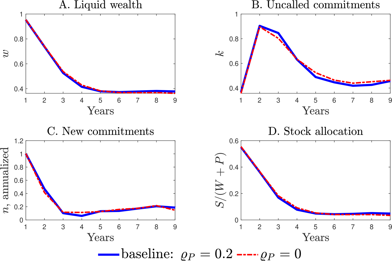
Figure 18: PE return autocorrelation and life cycle dynamics. The solid and dashed lines plot the average lifecycle outcomes under (1) our baseline model, and (2) a model where the PE returns process has zero autocorrelation but otherwise have the same return moments.

Figure˜18 compares the resulting difference in life cycle dynamics between the baseline case and the case where the LP ignores serial correlation in PE returns. We see that the LP’s portfolio allocations appear near-identical across the two cases. Furthermore, the two outcomes remain near-identical when we further condition outcomes on the macroeconomic state (see Figure˜D.1 in Appendix D).

The results in this section show that for long-term investors, the presence of serial correlation in PE returns may not be a critical factor in determining optimal portfolio allocations.

4.6 Risk budget

The risk weights in our baseline calibration $\theta_{S}=\theta_{P}=1.5$ correspond to 50% risk charges for PE and stocks (the risk budget threshold $\overline{\theta}$ is normalized to 1). In this section, we conduct comparative static exercises to investigate how the LP’s outcomes depend on these risk charges. This is a useful exercise in at least two contexts. First, while risk charges of 50% are representative numbers on average, risk charges can vary widely depending on asset quality. For example, S&P Global assesses anywhere between 35% to 99% market risk charges for equities depending on asset quality (S&P Global, 2023, Table 14). Second, individual LPs may assess different risk charges based on their own individual circumstances. For example, an insurer may assess higher risk charges for its PE investments depending on properties of its insurance portfolio; the risk weights $\theta_{P}$ and $\theta_{S}$ can then be interpreted as effective risk charges whose values depend on the riskiness of other components of the insurer’s balance sheet.

We demonstrate the effects of risk charges through two scenarios. In the first scenario, we set $\theta_{S}=\theta_{P}=2$, so that risk charges are uniformly higher. In the second scenario, we increase the risk charge for PE to $\theta_{P}=2$ while keeping $\theta_{S}=1.5$ unchanged. For both scenarios, we take the remaining parameters from the baseline calibration in Table˜1.

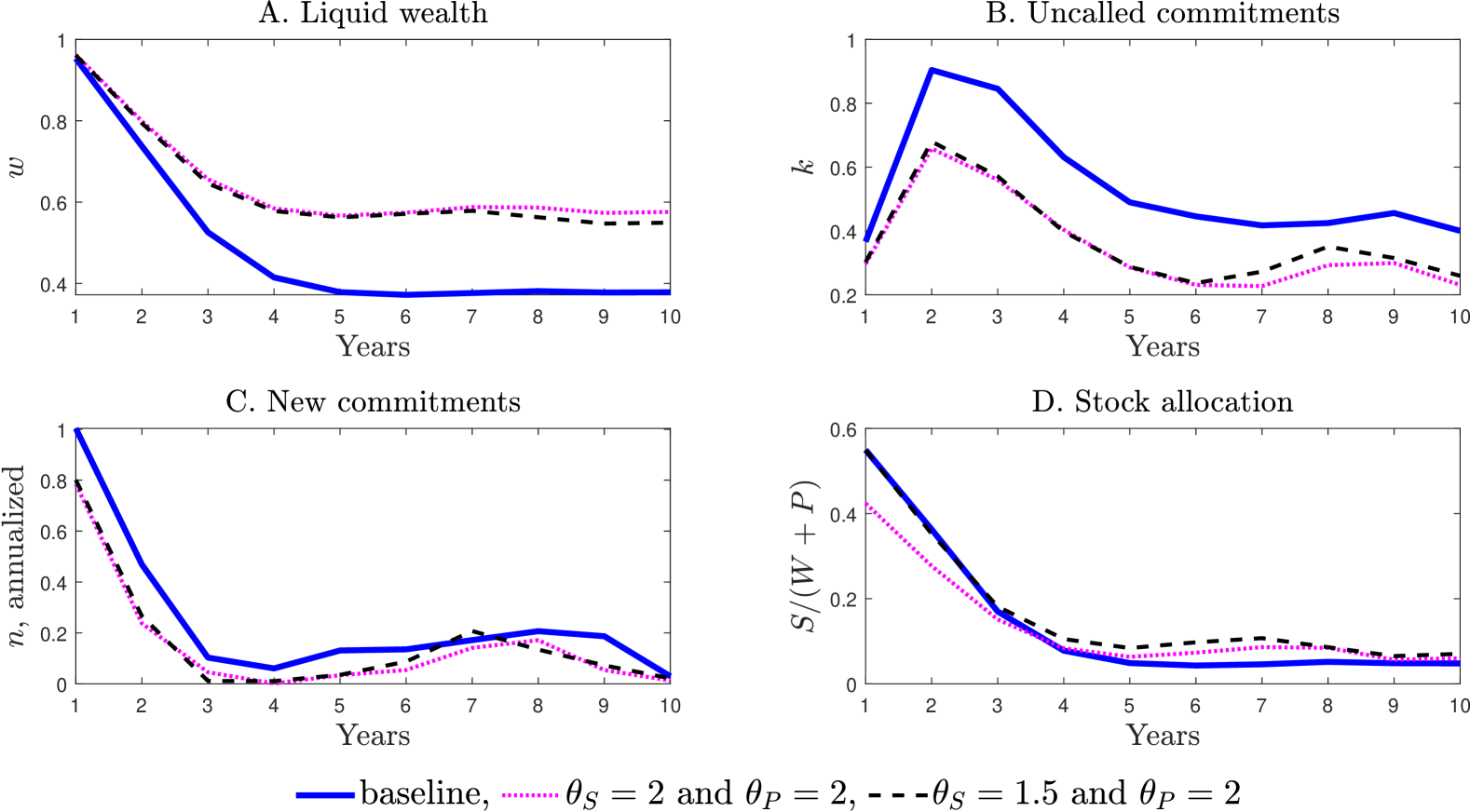
Figure 19: Life cycle dynamics under different risk charges. This figure displays average life cycle outcomes under alternative risk charges. For reference, the solid line plots outcomes under the baseline calibration in which $\theta_{P}=\theta_{S}=1.5$. The dotted line plots outcomes when both $\theta_{S}$ and $\theta_{P}$ equal 2, and the dashed line plots outcomes when only $\theta_{P}$ is increased to 2.

Figure˜19 illustrates the impact of risk charges on average life cycle outcomes. Compared to the baseline outcome (solid line), we see that overall allocations to PE and stocks are lower under the first scenario (dotted line) in which the risk charges for both PE and stocks are increased to $\theta_{P}=\theta_{S}=2$. For instance, during the initial ramp-up phase, uncalled commitments peak at 66% of total wealth in year 2, as opposed to 90% in the baseline calibration. Similarly, stock allocation in year 1 is reduced to 42% of total wealth on average compared to 55% in the baseline. In the maintenance phase from year 5 onwards, the PE allocation is 42% of total wealth, down from 62% in the baseline. The LP does, however, compensates with a slightly higher stock allocation during the maintenance phase: 7% of total wealth on average compared to 5% on average for the baseline. Figure˜D.2 in Appendix˜D additionally displays outcomes for the first scenario after further conditioning on the business cycle.

The second scenario isolates the effect of risk charges by only increasing $\theta_{P}$. In this case, we see from Figure˜19 that only PE allocations are affected to first order. Specifically, the average outcome for stock allocation remains roughly unchanged from the baseline (compare the solid and dashed lines in panel D) while the outcomes for PE allocation are similar to that under the first scenario (compare the dotted and dashed lines in panels A, B, and C). Figure˜D.3 in Appendix˜D additionally displays outcomes for the second scenario after further conditioning on the business cycle.

Figure 20: Total wealth outcomes under different risk charges. This figure illustrates the distribution of total wealth outcomes at the end of the investment horizon $t=T$. The initial total wealth is $W_{0}+P_{0}=1$. Panel A plots the distribution for total wealth $W_{T}+P_{T}$. Panel B plots the distribution for the realized growth in total wealth per annum, $\log(W_{T}+P_{T})/10$. Both panels compare outcomes under (1) the baseline in which $\theta_{P}=\theta_{S}=1.5$, (2) scenario 1 in which both $\theta_{P}$ and $\theta_{S}$ are increased to 2, and (3) scenario 2 in which only $\theta_{P}$ is increased to 2.

Figure˜20 compares the distribution of final outcomes under the different risk charge scenarios. We see that higher risk charges do indeed decrease the riskiness of the LP’s overall portfolio. For example, the standard deviation of annualized realized returns decreases to 2.35% (from the baseline value of 2.78%) under the second scenario when $\theta_{P}$ increases to 2; it further decreases to 2.14% under the first scenario when both $\theta_{P}$ and $\theta_{S}$ increase to 2. This decrease in risk does come at the expense of lower returns. The average annualized return decreases to 7.08% under the second scenario (down from 8.41% for the baseline), and further decreases to 6.79% under the first scenario.

The costs of imposing higher risk charges in certainty equivalent terms are as follows. Increasing $\theta_{P}$ alone to 2 (i.e., scenario 2) reduces the certainty equivalent wealth from the baseline value of 2.25 to 2.00 or, equivalent, a 11% reduction in certainty equivalent wealth. When we additionally increase $\theta_{S}$ to 2 (i.e., scenario 1), the certainty equivalent wealth further decreases to 1.92 for a 15% reduction in certainty equivalent wealth compared to the baseline.

5 Conclusion

Exciting recent developments in machine learning have enabled the solution of portfolio choice problems featuring higher dimensionality, more realistic trading frictions, and more complex constraints. In this paper, we employ Deep Kernel Gaussian Processes to accurately characterize the optimal policies in a private asset allocation model that incorporates a host of real-world complexities, including illiquidity, commitment lags, serial correlation in returns, business cycle fluctuations, and regulation-induced constraints. Our approach not only provides novel insights into private equity investing but also offers a flexible blueprint for tackling similarly challenging problems in economics and finance that involve substantial nonlinearities and a large number of state variables.

Appendix

Appendix A Specification for expected PE returns

In this section, we use the Getmansky, Lo, and Makarov (2004) model of smoothed returns for illiquid alternative investments to motivate our specification (14) for PE expected returns.

Applied to our context, the Getmansky, Lo, and Makarov (2004, equation 21) model posits that the observed return on PE investments $\log(R_{P,t+1})$ is a weighted average of contemporaneous and lagged values of the true but unobserved return on PE investments:

$$\log(R_{P,t+1})=\omega_{0}\log(\widetilde{R}_{P,t+1})+\omega_{1}\log(\widetilde{R}_{P,t})+...+\omega_{k}\log(\widetilde{R}_{P,t+1-k}),$$ (A.1)

In terms of notation for this section, we use a tilde to denote quantities associated with the true but unobserved returns. For example, $\log(R_{P,t+1})$ is the observed PE return at $t+1$ while $\log(\widetilde{R}_{P,t+1})$ is the unobserved contemporaneous true return. The coefficients $\omega_{j}$ in equation (A.1) are positive weights that sum to 1. We use the geometric weighting scheme considered in Getmansky, Lo, and Makarov (2004, equation 43):

$$\omega_{0}=(1-\phi)/(1-\phi^{k+1}),\quad\omega_{j}=\omega_{0}\phi^{j}\mbox{ for }j=1,...,k,$$ (A.2)

where $\phi\in(0,1)$. This weighting scheme leads to the convenient AR(1) process for the expected returns on observed PE returns (14).

Specifications (A.1) and (A.2) imply that the expected return for observed PE returns $\mu_{P,t}\equiv\mathbb{E}_{t}[\log(R_{P,t+1})]$ evolves as follows:

$$\mu_{P,t} =\omega_{0}\mathbb{E}_{t}[\log(\widetilde{R}_{P,t+1})]+\phi\mathbb{E}_{t}[\omega_{0}\log(\widetilde{R}_{P,t})+...+\omega_{0}\phi^{k-1}\log(\widetilde{R}_{P,t+1-k})]$$

$$=\omega_{0}\mathbb{E}_{t}[\log(\widetilde{R}_{P,t+1})]+\phi\mathbb{E}_{t}[\log(R_{P,t})-\omega_{0}\phi^{k}\log(\widetilde{R}_{P,t-k})]$$

$$=\omega_{0}\widetilde{\mu}_{P,t}+\phi\log(R_{P,t})-\omega_{0}\phi^{k+1}\mathbb{E}_{t}[\log(\widetilde{R}_{P,t-k})]$$ (A.3)

$$\approx\omega_{0}\widetilde{\mu}_{P,t}+\phi\log(R_{P,t})$$ (A.4)

$$=\omega_{0}\widetilde{\mu}_{P,t}+\phi\mu_{P,t-1}+\phi\sigma_{P,t-1}\varepsilon_{P,t}.$$ (A.5)

Equation (A.3) is a direct consequence of specifications (A.1) and (A.2); $\widetilde{\mu}_{P,t}\equiv\mathbb{E}_{t}[\log(\widetilde{R}_{P,t+1})]$ is the expected return for the true return process. The approximation (A.4) holds if $k$ is large enough or if $\phi$ is small enough. Equation (A.5) writes the observed return as $\log(R_{P,t})=\mu_{P,t-1}+\sigma_{P,t-1}\varepsilon_{P,t}$ where $\mu_{P,t-1}\equiv\mathbb{E}_{t-1}\left[\log(R_{P,t})\right]$, $\sigma_{P,t-1}\equiv\sqrt{Var_{t-1}\left[\log(R_{P,t})\right]}$, and $\varepsilon_{P,t}\equiv\left(\log(R_{P,t})-\mu_{P,t-1}\right)/\sigma_{P,t-1}$. Comparing equation (A.5) to equation (14), we see that the AR(1) process for expected PE returns (14) is a more flexible version of equation (A.5) in which the loading on the $\sigma_{P,t-1}\varepsilon_{P,t}$ term is allowed to differ from the autoregressive coefficient.

We make further functional form assumptions in our implementation. Specifically, the specification in equations (12) and (14) assumes (1) the expected true return $\widetilde{\mu}_{P,t}=\widetilde{\mu}_{P}(s_{t})$ depends only on the macroeconomic state (hence $\nu_{P}(s_{t})$ in equation (14) corresponds to the $\omega_{0}\widetilde{\mu}_{P,t}$ term from equation (A.5)), (2) the volatility of observed PE returns $\sigma_{P,t-1}=\sigma_{P}(s_{t-1})$ depends only on the macroeconomic state, and (3) the shock to observed PE returns $\varepsilon_{P,t}\sim\mathcal{N}(0,1)$ is normally distributed.

Appendix B Scaled value functions

Scaled choice variables.

We work with the following scaled versions of the choice variables:

$$n \equiv\frac{N}{W+P},$$ (B.1)

$$\widetilde{\phi}_{S} \equiv\frac{S+\gamma_{S}(W+P)\left(\frac{S}{W+P}\right)^{2}}{W-\gamma_{N}(W+P)\left(n-\overline{n}\right)^{2}}.$$ (B.2)

Here, $n$ is the new PE commitments scaled by total wealth. The interpretation for $\widetilde{\phi}_{S}$ is as follows. The denominator in equation (B.2) is the amount of liquid wealth that is available to be invested in stocks and bonds after deducting adjustment costs for new PE commitments from current liquid wealth. Of this amount, $\widetilde{\phi}_{S}$ is the fraction invested in stocks inclusive of stock adjustment costs. We also denote by

$$\phi_{S}\equiv\frac{S}{W-\gamma_{N}(W+P)\left(n-\overline{n}\right)^{2}}.$$ (B.3)

the fraction invested in stocks excluding stock adjustment costs. The relation between $\widetilde{\phi}_{S}$ and $\phi_{S}$ is

$$\phi_{S}=\frac{-1+\sqrt{1+4\gamma_{S}[w-\gamma_{N}(n-\overline{n})^{2}]\widetilde{\phi}_{S}}}{2\gamma_{S}[w-\gamma_{N}(n-\overline{n})^{2}]}.$$ (B.4)

Scaled value function in default.

The recursive formulation for the scaled value function in default is

$$v_{D}(t,s)=\max_{\widetilde{\phi}_{S}\in[0,\widetilde{\phi}_{S,max}(s)]}\mathbb{E}\left[\left(g_{D}^{\prime}\right)^{1-\gamma}|s\right]^{\frac{1}{1-\gamma}}\mathbb{E}\left[v_{D}(t+1,s^{\prime})^{1-\gamma}|s\right]^{\frac{1}{1-\gamma}}$$ (B.5)

where

$$g_{D}^{\prime}\equiv\frac{W^{\prime}}{W}=R_{S}^{\prime}\phi_{S}+R_{f}(s)\left(1-\widetilde{\phi}_{S}\right)-\Gamma(\theta_{S}\widetilde{\phi}_{S})$$ (B.6)

is the growth rate of total wealth in default and

$$v_{D}(T,s)=1$$

is the terminal condition. Note that when computing the scaled value function (B.5), equations (B.2), (B.3), and (B.4) for $\widetilde{\phi}_{S}$, $\phi_{S}$, and their relation, respectively, are computed with $P=0$ and $n=0$. In addition, note that while the $\mathbb{E}\left[u_{D}(t+1,s^{\prime})^{1-\gamma}|s\right]^{\frac{1}{1-\gamma}}$ on the right-hand side of equation (B.5) affects the scaled value function, it does not affect the optimal portfolio choice. This is because the growth rate of total wealth (B.6) does not depend on $s^{\prime}$. As a result, the optimal policies in default only depend on the macroeconomic state $s$.

The upper bound $\widetilde{\phi}_{S,max}(s)\equiv\sup\left\{\widetilde{\phi}_{S}\in[0,1]:\;\inf_{R_{S}^{\prime}}g_{D}^{\prime}=R_{f}(s)\left(1-\widetilde{\phi}_{S}\right)-\Gamma(\theta_{S}\widetilde{\phi}_{S})\right\}$ appearing in problem (B.5) ensures that the growth in wealth $g_{D}^{\prime}$ is strictly positive so that utilities are well-defined. The upper bound equals

$$\widetilde{\phi}_{S,max}(s)=\left\{\begin{array}[]{ll}1&\mbox{if }\theta_{S}\leq\overline{\theta},\\ \min\left\{\frac{\overline{\theta}}{\theta_{S}}+\frac{-R_{f}(s)+\sqrt{R_{f}(s)^{2}+4\kappa\theta_{S}R_{f}(s)(\theta_{S}-\overline{\theta})}}{2\kappa\theta_{S}^{2}},1\right\}&\mbox{if }\theta_{S}>\overline{\theta}.\end{array}\right.$$ (B.7)

Similarly, the lower bound $\widetilde{\phi}_{S}\geq 0$ rules out shorting which is also necessary to ensure that utilities are well-defined.

Scaled value function before default.

The recursive formulation for the scaled value function before default is

$$v(t,w,k,\mu_{P},s)=\max_{n,\widetilde{\phi}_{S}}\mathbb{E}\left[\max\left\{g_{D}^{\prime}v_{D}\left(t+1,s^{\prime}\right),g^{\prime}v\left(t+1,w^{\prime},k^{\prime},\mu_{P}^{\prime},s^{\prime}\right)\right\}^{1-\gamma}\left|w,k,\mu_{P},s\right.\right]^{\frac{1}{1-\gamma}}$$ (B.8)

subject to

$$g_{D}^{\prime}= \,\left(1-w\right)\left[\lambda_{D}(s^{\prime})+\alpha(s^{\prime})(1-\lambda_{D}(s^{\prime}))\right]R_{P}^{\prime}-\Gamma(\theta_{D})$$

$$+\left[w-\gamma_{N}(n-\overline{n})^{2}\right]\left[\phi_{S}R_{S}^{\prime}+(1-\widetilde{\phi}_{S})R_{f}(s)\right],$$

$$\theta_{D}= \,\frac{\theta_{S}\left[w-\gamma_{N}(n-\overline{n})^{2}\right]\widetilde{\phi}_{S}}{1-\gamma_{N}(n-\overline{n})^{2}},$$

$$g^{\prime}= \,(1-w)R_{P}^{\prime}+\left[w-\gamma_{N}(n-\overline{n})^{2}\right]\left[\phi_{S}R_{S}^{\prime}+(1-\widetilde{\phi}_{S})R_{f}(s)\right]-\Gamma(\theta),$$ (B.9)

$$\theta= \,\frac{\theta_{P}(1-w)+\theta_{S}\left[w-\gamma_{N}(n-\overline{n})^{2}\right]\widetilde{\phi}_{S}}{1-\gamma_{N}(n-\overline{n})^{2}},$$

$$k^{\prime}= \,\frac{[1-\lambda_{K}(s^{\prime})]k+[1-\lambda_{N}(s^{\prime})]n}{g^{\prime}},$$

$$w^{\prime}= \,\frac{\left\{\begin{array}[]{c}\lambda_{D}(s^{\prime})R_{P}^{\prime}(1-w)-\lambda_{K}(s^{\prime})k-\lambda_{N}(s^{\prime})n-\Gamma(\theta)\\ +\left[w-\gamma_{N}(n-\overline{n})^{2}\right]\left[\phi_{S}R_{S}^{\prime}+(1-\widetilde{\phi}_{S})R_{f}(s)\right]\end{array}\right\}}{g^{\prime}},$$ (B.12)

$$\mu_{P}^{\prime}= \,\varrho_{P,1}\mu_{P}+\varrho_{P,2}\log R_{P}^{\prime}+\nu_{P}(s^{\prime}),$$

$$n\in \,[n_{min}(w),n_{max}(w)],\quad\widetilde{\phi}_{S}\in[0,\widetilde{\phi}_{S,max}(w,n,s)],$$ (B.13)

with terminal condition

$$v\left(T,w,k,\mu_{P},s\right)=1.$$

Here, $g_{D}^{\prime}=W_{D}^{\prime}/(W+P)$ and $g^{\prime}=(W^{\prime}+P^{\prime})/(W+P)$ denote the growth rates of total wealth conditional on defaulting and not defaulting, respectively.

The limits on the choice variables (B.13) ensure that utility is well-defined. To see why, note that the log returns on PE and the stock are normally distributed and are therefore unbounded. Hence, this would require $\max\{g_{D}^{\prime},g^{\prime}\}>0$ for all realization of return shocks. This condition implies $\inf g_{D}^{\prime}=[w-\gamma_{N}(n-\overline{n})^{2}](1-\widetilde{\phi}_{S})R_{f}(s)-\Gamma(\theta_{D})\geq 0$ where the infimum is taken over both $R_{P}^{\prime}$ and $R_{S}^{\prime}$. From this, we obtain

$$n_{min}(w)=\max\left\{\overline{n}-\sqrt{\frac{w}{\gamma_{N}}},0\right\},\quad n_{max}(w)=\overline{n}+\sqrt{\frac{w}{\gamma_{N}}},$$

and

$$\widetilde{\phi}_{S,max}(w,n,s)$$

$$= \left\{\begin{array}[]{ll}1&\mbox{if }\widetilde{\theta}_{S}(w,n)\leq\overline{\theta},\\ \min\left\{\frac{\overline{\theta}}{\widetilde{\theta}_{S}(w,n)}+\frac{-\widetilde{R}_{f}(w,n,s)+\sqrt{\widetilde{R}_{f}(w,n,s)^{2}+4\kappa\widetilde{\theta}_{S}(w,n)\widetilde{R}_{f}(w,n,s)\left[\widetilde{\theta}_{S}(w,n)-\overline{\theta}\right]}}{2\kappa\widetilde{\theta}_{S}(w,n)^{2}},1\right\}&\mbox{if }\widetilde{\theta}_{S}(w,n)>\overline{\theta},\end{array}\right.$$

where

$$\widetilde{\theta}_{S}(w,n)\equiv\frac{\theta_{S}[w-\gamma_{N}(n-\overline{n})^{2}]}{1-\gamma_{N}(n-\overline{n})^{2}},\quad\mbox{and }\widetilde{R}_{f}(w,n,s)\equiv[w-\gamma_{N}(n-\overline{n})^{2}]R_{f}(s).$$

Scaled value function for the heuristic problem (27).

The value function for the heuristic problem (27) can be scaled as $V_{\mbox{heuristic}}(t,W_{total},s)=\left[W_{total}v_{\mbox{heuristic}(t,s)}\right]^{1-\gamma}/(1-\gamma)$ where $v_{\mbox{heuristic}}$ solves

$$v_{\mbox{heuristic}}(t,s)=\max_{\phi_{S},\phi_{P}}\mathbb{E}\left[\left(g_{total}^{\prime}\right)^{1-\gamma}|s\right]^{\frac{1}{1-\gamma}}\mathbb{E}\left[v_{\mbox{heuristic}}(t+1,s^{\prime})^{1-\gamma}|s\right]^{\frac{1}{1-\gamma}}$$ (B.14)

subject to

$$g_{total}^{\prime}\equiv\frac{W_{total}^{\prime}}{W_{total}} =R_{S}^{\prime}\phi_{S}+R_{P}^{\prime}\phi_{P}+R_{f}(s)\left(1-\phi_{S}-\phi_{P}\right)-\Gamma(\theta_{S}\phi_{S}+\theta_{P}\phi_{P}),$$

$$\phi_{S},\phi_{P} \in[0,1],$$

$$\phi_{S}+\phi_{P} =1$$

and the terminal condition $v_{\mbox{heuristic}}(T,s)=1$.

Appendix C Numerical Implementation

We first solve the scaled problem in default (B.5). In doing so, we note that the the value function can be split as

$$v_{D}(t,s)=\mathbb{E}\left[\left(u_{D}(t+1,s^{\prime})\right)^{1-\gamma}|s\right]^{\frac{1}{1-\gamma}}\max_{\widetilde{\phi}_{S}\in[0,\widetilde{\phi}_{S,max}(s)]}\mathbb{E}\left[\left(g_{D}^{\prime}\right)^{1-\gamma}|s\right]^{\frac{1}{1-\gamma}}.$$ (C.1)

This is because $g_{D}^{\prime}$ does not depend on $s^{\prime}$ (see equation (B.6)). Hence, the optimal portfolio choice problem depends $s$ alone and is obtained by solving

$$\max_{\widetilde{\phi}_{S}\in[0,\widetilde{\phi}_{S,max}(s)]}\mathbb{E}\left[\left(g_{D}^{\prime}\right)^{1-\gamma}|s\right]^{\frac{1}{1-\gamma}}.$$ (C.2)

To ensure numerical accuracy, we use adaptive quadrature in to compute expectations.

After obtaining $v_{D}(t,s)$, we solve the scaled problem before default (see equation (B.8)) using backward induction. The procedure is as follows:

1. Initiate the value function at $t=T$ using the terminal condition $v\left(T,w,k,\mu_{P},s\right)=1$.

2. Obtain sample points for the state variables $(w,k,\mu_{P})$. In doing so, we sample 800 points via a Halton sequence over the hypercube $\{(w,k,\mu_{P}):\;w\in[0,1],k\in[01.5],\mu_{P}\in[\mu_{P,lb},\mu_{P,ub}]\}$ where the bounds $\mu_{P,lb}$ and $\mu_{P,ub}$ are set to be the 0.1st and 99.9th percentiles of the stationary distribution for $\mu_{P}$, respectively.

3. Given a value function $v_{GP}\left(t+1,w,k,\mu_{P},s\right)$ that has been previously fitted via Deep Kernel Gaussian Process Regression, do the following:

   1. For each $s$ at time $t$, solve problem (B.8) for the sample points for $(w,k,\mu_{P})$ obtained in step 2. When doing so, we use the fitted value function $v_{GP}\left(t+1,\cdot\right)$ as the continuation value when not defaulting next period. As in the problem after default, we use adaptive quadrature to compute expectations to ensure numerical accuracy. To ensure that we find a global maximum, we first consider a coarse grid of policy points. We then run an interior-point optimization algorithm starting from the best policy based on the coarse grid. The end result is a set of observations for the value and policy functions at the sample points.

   2. We use the observations from step (a) to fit deep kernel Gaussian processes for the value and policy functions at time $t$ for each state $s$. Our choice for the deep kernel (24) is as follows. The neural network component $NN$ takes the three-dimensional input $(w,k,\mu_{P})$ and passes it through 3 hidden layers with 64, 32, and 16 units, respectively, before outputting 2 features (the shape of the hidden layers follow a so-called “decoder structure”); we use Gaussian error linear unit (GELU) activation. These 2 output features are then passed through a Matern 5/2 kernel (20). We train the parameters of the deep kernel Gaussian processes by maximizing the marginal likelihood (23) using the Adam optimizer (Kingma and Ba, 2015) with a learning rate of 0.001. To ensure that the training converges to a global optimum, we run the Adam optimizer 10 times from different initial points. We always use the trained parameters from step $t+1$ as one of the initial points; the remaining initial points are randomly drawn with Xavier initialization for the neural network weights. We standardize both input and output variables when training.

4. Repeat step 3 until $t=0$.

Figure˜6(b) and Figure˜C.1 illustrate the value function and policy functions at $t=0$, respectively.

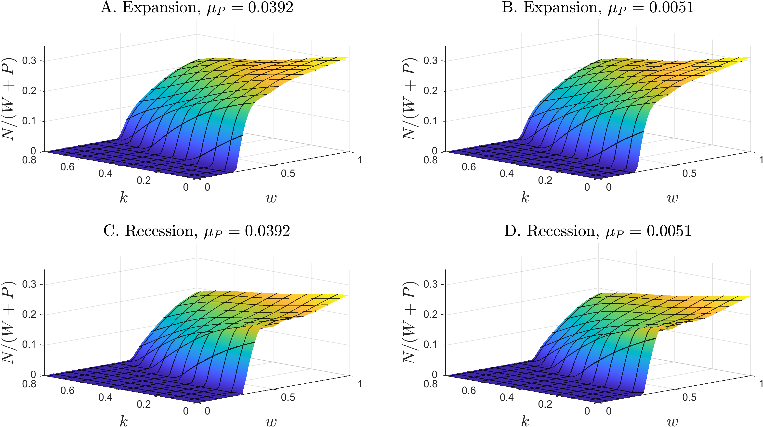
(a) New commitments.

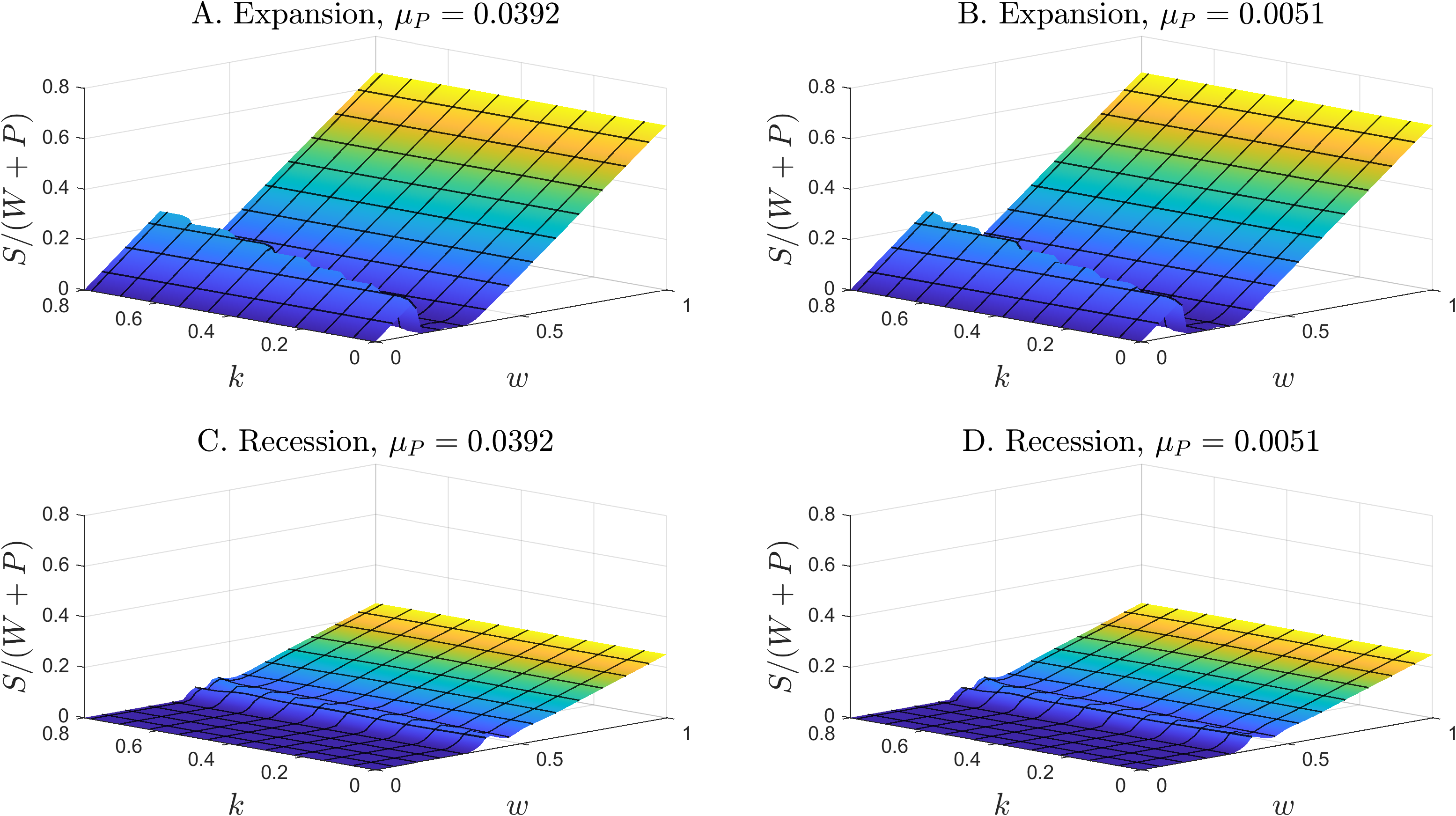
(b) Stock allocation.

Figure C.1: Policies at $t=0$.

Heuristic portfolio choice problem.

Appendix D Additional Figures

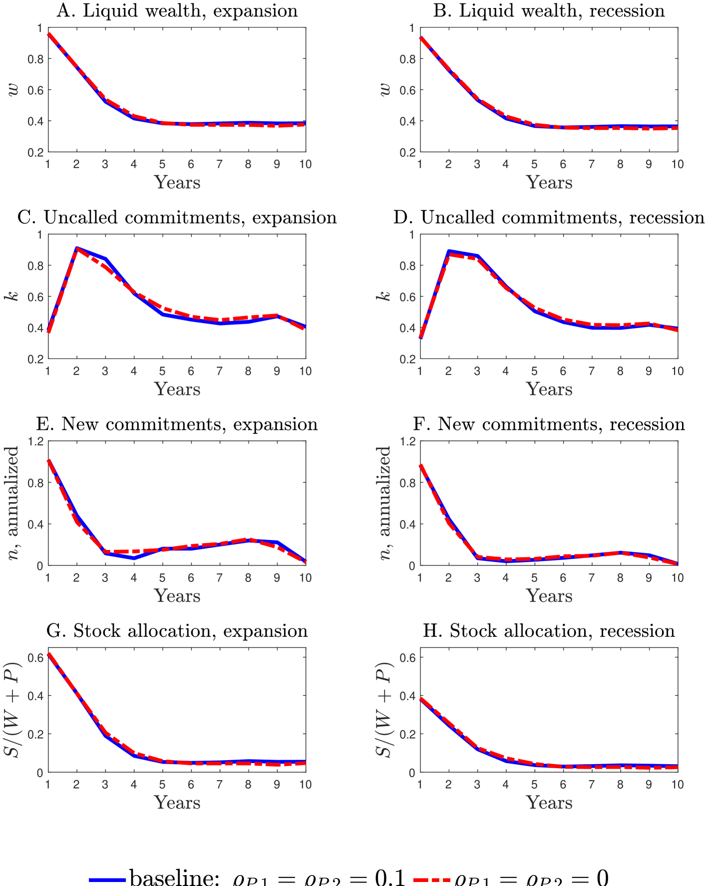
Figure D.1: Life cycle comparison (conditional), PE return autocorrelation. The solid and dashed lines plot the average lifecycle outcomes under (1) our baseline model, and (2) a model where the PE returns process has zero autocorrelation but otherwise have the same return moments.

Figure D.2: Life cycle comparison (conditional), risk budget 1.

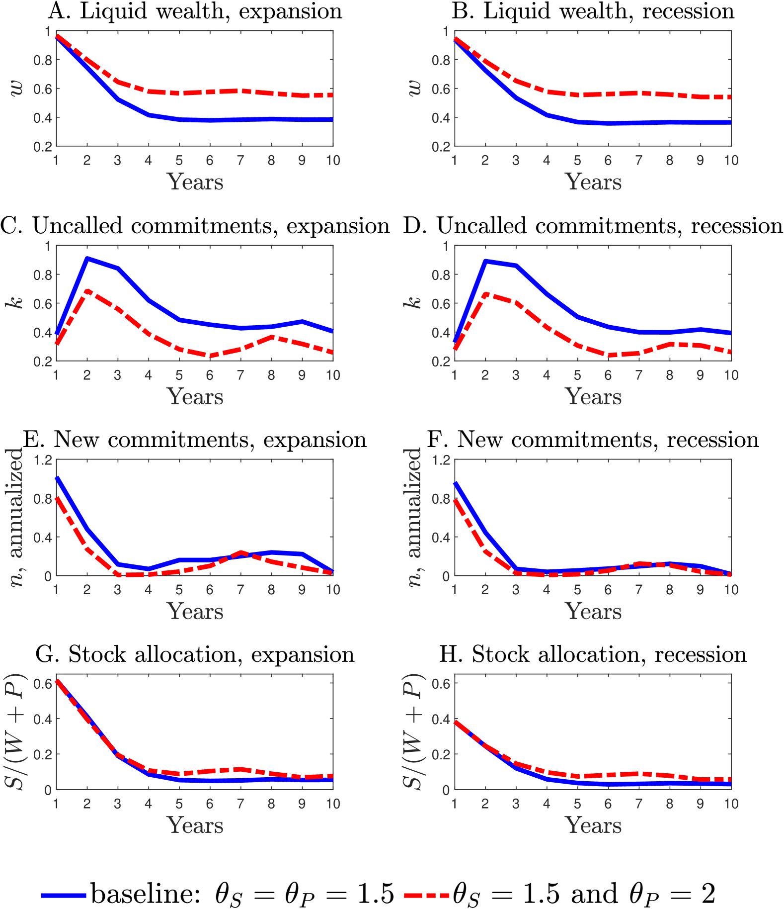
Figure D.3: Life cycle comparison (conditional), risk budget 2.

References

- (1)
- Ang, Papanikolaou, and Westerfield (2014) Ang, A., D. Papanikolaou, and M. Westerfield, 2014, “Portfolio Choice with Illiquid Assets,” Management Science, 60, 2737–2761.
- Bolton, Chen, and Wang (2011) Bolton, P., H. Chen, and N. Wang, 2011, “A Unified Theory of Tobin’s , Corporate Investment, Financing, and Risk Management,” Journal of Finance, 66, 1545–1578.
- Bolton, Chen, and Wang (2013) Bolton, P., H. Chen, and N. Wang, 2013, “Market Timing, Investment, and Risk Management,” Journal of Financial Economics, 109, 40–62.
- Dimmock, Wang, and Yang (2024) Dimmock, S. G., N. Wang, and J. Yang, 2024, “The Endowment Model and Modern Portfolio Theory,” Management Science, 70, 1554–1579.
- Duarte, Duarte, and Silva (2024) Duarte, V., D. Duarte, and D. H. Silva, 2024, “Machine Learning for Continuous-Time Finance,” Review of Financial Studies, 37, 3217–3271.
- Duarte, Fonseca, Goodman, and Parker (2022) Duarte, V., J. Fonseca, A. S. Goodman, and J. A. Parker, 2022, “Simple Allocation Rules and Optimal Portfolio Choice Over the Lifecycle,” Working Paper 29559, National Bureau of Economic Research.
- Eling and Holzmuller (2008) Eling, M., and I. Holzmuller, 2008, “An Overview and Comparison of Risk-Based Capital Standards,” Journal of Insurance Regulation, 26.
- Gaegauf, Scheidegger, and Trojani (2023) Gaegauf, L., S. Scheidegger, and F. Trojani, 2023, “A comprehensive machine learning framework for dynamic portfolio choice with transaction costs,” Working Paper.
- Geltner (1991) Geltner, D. M., 1991, “Smoothing in appraisal-based returns,” Journal of Real Estate Finance and Economics, 4, 327–345.
- Getmansky, Lo, and Makarov (2004) Getmansky, M., A. W. Lo, and I. Makarov, 2004, “An econometric model of serial correlation and illiquidity in hedge fund returns,” Journal of Financial Economics, pp. 529–609.
- Giommetti and Sorensen (2024) Giommetti, N., and M. Sorensen, 2024, “Optimal Allocation to Private Equity,” Working Paper.
- Gourier, Phalippou, and Westerfield (2024) Gourier, E., L. Phalippou, and M. Westerfield, 2024, “Capital Commitment,” Journal of Finance, 79, 3407–3457.
- Kingma and Ba (2015) Kingma, D. P., and J. Ba, 2015, “Adam: A Method for Stochastic Optimization,” arXiv preprint arXiv:1412.6980.
- Korteweg and Westerfield (2022) Korteweg, A., and M. M. Westerfield, 2022, “Asset Allocation with Private Equity,” Foundations and Trends(R) in Finance, 13, 95–204.
- McKinsey & Company (2024) McKinsey & Company, 2024, “McKinsey Global Private Markets Review 2024: Private markets: A slower era,” Discussion paper, McKinsey & Company.
- Nadauld, Sensoy, Vorkink, and Weisbach (2019) Nadauld, T. D., B. A. Sensoy, K. Vorkink, and M. S. Weisbach, 2019, “The liquidity cost of private equity investments: Evidence from secondary market transactions,” Journal of Financial Economics, 132, 158–181.
- Neuberger Berman (2022) Neuberger Berman, 2022, “The Historical Impact of Economic Downturns on Private Equity,” Discussion paper, Neuberger Berman.
- Rasmussen and Williams (2005) Rasmussen, C. E., and C. K. I. Williams, 2005, Gaussian Processes for Machine Learning, The MIT Press.
- Renner and Scheidegger (2018) Renner, P., and S. Scheidegger, 2018, “Machine Learning for Dynamic Incentive Problems,” Working Paper.
- Scheidegger and Bilionis (2019) Scheidegger, S., and I. Bilionis, 2019, “Machine learning for high-dimensional dynamic stochastic economies,” Journal of Computational Science, 33, 68 – 82.
- Sorensen, Wang, and Yang (2014) Sorensen, M., N. Wang, and J. Yang, 2014, “Valuing Private Equity,” Review of Financial Studies, 27, 1977–2021.
- S&P Global (2023) S&P Global, 2023, “Insurer Risk-Based Capital Adequacy Methodology And Assumptions,” https://www.spglobal.com/ratings/en/research/articles/231115-criteria-insurance-general-insurer-risk-based-capital-adequacy-methodology-and-assumptions-12862217, Accessed: January 2025.
- Takahashi and Alexander (2002) Takahashi, D., and S. Alexander, 2002, “Illiquid Alternative Asset Fund Modeling,” Journal of Portfolio Management, 28, 90–100.
- Wilson, Hu, Salakhutdinov, and Xing (2016) Wilson, A. G., Z. Hu, R. Salakhutdinov, and E. P. Xing, 2016, “Deep Kernel Learning,” in Arthur Gretton, and Christian C. Robert (ed.), Proceedings of the 19th International Conference on Artificial Intelligence and Statistics, , vol. 51 of Proceedings of Machine Learning Research, pp. 370–378, Cadiz, Spain. PMLR.