Generic Antiholomorphic Polymonial Vector Fields
Abstract.
An analytic classification of generic anti-polynomial vector fields is given in term of a topological and an analytic invariant. The number of generic strata in the parameter space is counted for each degree of . A Realization Theorem is established for each pair of topological and analytic invariants. The non-generic case of a maximal number of heteroclinic connections is also given a classification. The bifurcation diagram for the quadratic case is presented.
Key words and phrases:
Antiholomorphic polynomial vector fields, noncrossing trees, classification, combinatorial invariant, analytic invariant1991 Mathematics Subject Classification:
37F20; 37C151. Introduction
In this paper, we are mainly concerned with the study and classification of vector fields , where is a polynomial (and is the complex conjugation). By classifying, we mean describing the equivalence classes of the family of vector fields under some equivalence relation, such as the topological orbital equivalence or a holomorphic or antiholomorphic equivalence.
There are several motivations for this study. Early in the development of complex analysis, complex potentials found many applications in physics; broadly speaking, given a (possibly ramified) holomorphic function (the complex potential), over some open set , the dynamics of may be thought of as the laminar flow of a Newtonian fluid in the plane. Although the flow of a real fluid is much more complicated than this, these simple potential flows can be used to construct a variety of flows, by superposition, patching or otherwise, that are much closer to what is observed in the physical world. Potential flows have been used in the early development of aerodynamics [VD75] and in recent work (e.g. [CKM+17]). From this point of view, (generic) anti-holomorphic polynomials arise as flows on for which the complex potential
-
•
is meromorphic on the whole Riemann;
-
•
and has only simple zeroes in and no homoclinic loops or heteroclinic connections.
Such a flow with stagnation point is characterized at the topological level by the organization of strips (zone isomorphic to horizontal strip) in which the fluid flows from infinity to infinity. In Section 3, we prove that there such configurations, where is the number of non crossing trees with vertices modulo rotations of order . Then the circulation and the flux of each strip determines analytically the polynomial.
There has also been recent development in approximation of potential flows in planar domains [Bad20]. Rational functions are used to approximate the flow. The method uses a cluster of poles near the corner to achieve very fast approximation when the number of poles increases exponentially. Recent work [Tre24] on the approximation of solutions of the Laplace equation in planar domains showed that rational approximations performs better than polynomial approximations on some non-convex regions.
A structurally stable anti-polynomial (i.e. a polynomial in ) vector field has invariant regions isomorphic to a horizontal strip. The circulation and the flux across a transversal section of this region is an analytic invariant that helps to classify those vector fields.
The most degenerate singularity is often the organizing centre of the dynamics. The unfoldings of a multiple saddle point can be analyzed through the use of a family of anti-polynomials (i.e. polynomial in ) or, equivalently, a family of rational function of the form . The goal of the present paper is to classify families of generic anti-polynomials.
On a different note, we also see this work as part of the analysis of (holomorphic) polynomial vector fields on . Indeed, it is well known that such a vector field has a pole at infinity, which is the organizing centre of the dynamics. Those vector fields have been well-studied in [DES05] and then by [BD10]. To study the unfoldings of this singularity, it is natural to consider , which leads to by observing that
In other words, the dynamics of and have the same orbits, but differ by a time rescaling. In fact, in this paper, we will often consider both and , and use whichever one is more convenient given the context.
A different point of view can also be used to see this work as part of holomorphic dynamics. With the idea that , we can see the ODE as a system of two equations in
This family of systems is invariant under the symmetry . The dynamics studied in this paper corresponds to the dynamics for real time in the invariant plane in . See [Ily08] for more on analytic systems.
This article follows in the step of the visionary work of Douady, Estrada and Sentenac in their unpublished paper [DES05] on structurally stable polynomial vector fields, and later the work of Branner and Dias [BD10], expanding the analysis to every polynomial vector fields. The classification of real-coefficients polynomial vector fields has recently been studied in [GR25].
The paper is organized as follow. In Section 2, we study the separatrix graph and the two types of components in the complement of this graph. In Section 3, we discuss the topological properties of the phase portrait and we count the number of equivalence classes under topological orbital equivalence. Section 4 is devoted to the analytic invariants of the vector fields. In Section 5, we prove a realization theorem, proving that every phase portrait is completely determined by the topological and analytic invariants. Lastly, in Section 6, we initiate the study of non-structurally stable vector fields.
2. Description of the phase portrait
We consider the system
| (1) |
where is a monic and centred polynomial of degree . Near infinity, the behaviour of the dynamics is of the form , with and small (see Figure 1). Hence, the system has a parabolic point of codimension near the origin.
Through the paper, we will denote by the set of such vector fields and we will implicitly identify any such vector field with its defining polynomial.

The phase portrait may contain a finite number of simple saddle points, multiple saddle points and heteroclinic connections. The latter two are the only possible non-structurally stable objects. Indeed, any singular point must be a saddle point, so no nodes, parabolic points or centres are possible, and no homoclinic loops or limit cycles can exist, since they must have a positive index number. For the same reason, a domain cannot be bounded by orbits.
The basin of attraction of consists of a finite number of connected and simply connected regions of bounded by incoming orbits and singular points. If we know the basin of attraction at and its boundary, we can reconstruct the whole phase portrait. This allows us to reduce our problem to the study of the separatrix graph (defined in the following paragraph).
2.1. Separatrix graph
The separatrix graph, formed of singular points and separatrices, was already used in [DES05] in the case of holomorphic polynomial vector fields. So it is no surprise that this object completely determines the topological structure of the phase portrait in the case at hand. At the end of Section 2, we will reduce the study of the structurally stable phase portrait under topological orbital equivalence to that of different graphs, deduced from the separatrix graph, called noncrossing trees. The discrete and combinatorial properties of those trees were already studied in [Noy98].
Definition 2.1.
-
(1)
By abuse of language, we will use the term separatrix both for incoming and outgoing separatrices.
-
(2)
We will call separatrix graph of (1) the graph on the zeros of with the separatrices as edges.
Proposition 2.2.
The boundary of a connected component of has either one or two connected components. Each component of the the boundary contains at least one singular point. If the vector field is generic, then each component contains at most one singular point.
This motivates the following definition.
Definition 2.3.
A connected component of is said to be
-
(1)
a sepal zone if its boundary has two components;
-
(2)
a petal zone if its boundary has one component.
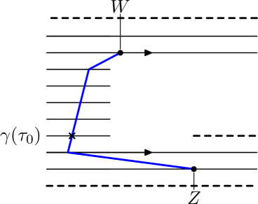
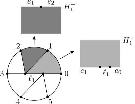
Here is the motivation for this terminology. A petal zone contains a petal of the parabolic point at infinity and is bounded by a single curve formed by the union of separatrices and single points. A sepal zone is a domain isomorphic to a strip that fits in the interstice spaces between petals. Note that in the rectifying coordinate , a sepal zone becomes a horizontal strip, and petal zone, an upper or lower half-plane.
Proof of Proposition 2.2.
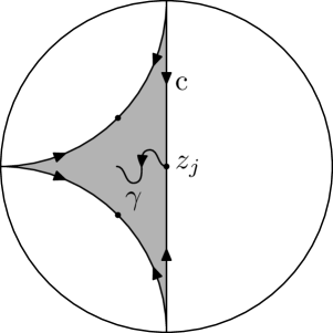
Let be a connected component of . It is clear that is a union of separatrices and singular points, since its boundary is contained in . Moreover, must be unbounded, since contains no cycle. We call an end of a connected region of for a very large . We want to prove that has either one end (then is a petal) or two ends (then is a sepal).
Suppose has more than two ends. First, we transform in the rectifying coordinate , where becomes . Note that extends to the boundary into a continuous function. Let be two points such that their -limit or their -limit goes in different ends. We can of course suppose that their -limit goes in different ends, otherwise it suffices to inverse time. We can join and by a polygonal arc transverse to the flow. See Figure 2. Let
Then the orbit of must land on the boundary so that the orbit of must land on one the boundaries, a contradiction.
∎
2.2. Structurally stable vector fields
We now specialize our study to the case of structurally stable vector fields, from here until Section 6. Broadly speaking, a vector field is structurally stable if its phase portrait remains topologically the same after a small perturbation. In the case of antiholomorphic polynomial vector fields, this is equivalent to having only simple singular points and no heteroclinic connection. (Limit cycles and homoclinic loops were already impossible in these systems.)
Now, consider the compactification of the complex plane given by a gnomonic projection on a half-sphere, so that is mapped on the lower half-sphere and the circle at infinity is mapped on the equator. (Note that this projection is not conformal, however we only use it for topological consideration.) We can divide the circle in attracting intervals, where orbits are landing at infinity, alternating with repulsive intervals, where orbits are leaving infinity. For convenience, we will identify each interval to a point , with an attractive (resp. repulsive) interval for even (resp. odd).
For structurally stable vector fields, the understanding of the phase portrait can be translated solely in combinatorial terms. The goal of the following discussion is to construct this so called combinatorial data.
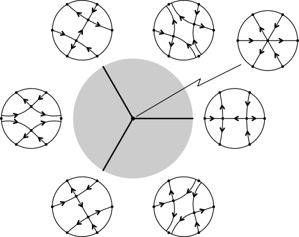
At each zero of , there are incoming (solid on Figure 3) and outgoing (dashed on Figure 3) orbits. These come in alternating order since every singularity is a saddle point. By the previous discussion, each incoming (resp. outgoing) separatrix must come from one of the directions escaping (resp. going toward) the point . Taking orientation into consideration, this gives points on and, identifying opposite separatrices to a single curve, edges (see Figure 3).

This data organizes the topological behaviour of the phase portrait. In fact, knowing only half of this information is sufficient. Indeed, if we are only given the information from the incoming separatrices, we can completely recover the (topological) data of the outgoing ones since singular points are saddle points and incoming separatrices determine the basin of attraction at (see Figure 3). In a similar fashion, the outgoing separatrices also determine the phase portrait.
We encode this data in a graph embedded in , having vertices on and edges. Note that if we consider both the incoming and outgoing graphs, we get the separatrix graph of the system (1). Remark also that given an incoming (resp. outgoing) graph, its associated outgoing (resp. incoming) graph is (isomorphic to) its dual (for the definition of the dual graph, we refer the reader to Definition 3.5). Hence, we’ll refer to the incoming graph as the combinatorial invariant of (1). This choice is arbitrary, i.e. it would have been equivalent to give the outgoing graph as the combinatorial invariant. We resume this discussion in the following results.
Lemma 2.4.
The dual of an incoming graph is its outgoing graph and . Moreover, the separatrix graph is given by and .
We now want to understand the structure of those graphs.
Lemma 2.5.
If is an incoming graph, then it’s embedded (i.e. no two vertices intersect).
Proof.
This follows from Cauchy’s uniqueness theorem. Two crossing edges would result from crossing separatrices. ∎
Lemma 2.6.
If is an incoming graph, then has no cycle.
Proof.
By contradiction, assume that there exists a cycle and take any edge in the cycle. The edge corresponds to the two separatrices entering some zero . Now recall that there must exists an outgoing separatrix at that satisfies . But any point is in the basin of attraction of one of the ’s, giving a contradiction (see Figure 4).
∎
By combining the previous lemmas, we can count the number of sepal zones and petal zones in .
Proposition 2.7.
Let be a generic vector field of degree . The separatrix graph divides into sepal zones and petal zones.
Proof.
An incoming graph has edges, so it divides in connected, simply-connected components. In each component, there is a vertex of the dual tree on the circle at infinity. If is the incidence of the -th vertex of the dual, it means this connected component gets divided into connected components by the edges of the dual tree. Since the dual is the outgoing tree, it also has edges, so that . Therefore, the number of connected components of is .
Moreover, for each , the corresponding connected component is divided in two petal zones and sepal zones. Therefore, there are sepal zones and petal zones. ∎
3. Combinatorial invariant
Definition 3.1.
A noncrossing tree of order (or -nc tree for short) is a tree on vertices and edges that is embedded in such that every vertex belongs in and no two embedded vertices cross.
Denote by the relation of topological orbital equivalence on . By Lemmas 2.5 and 2.6, counting incoming graphs amounts to counting some nc trees. We have the following.
Theorem 3.2.
Let . There is a bijection between -nc trees and the equivalence classes of .
Proof.
One direction of the proof of Theorem 3.2 is given by the two lemmas that characterize the phase portrait of antiholomorphic polynomial vector fields. The other direction is a corollary of the Realization Theorem 5.1 which says that for each nc tree, there is a vector field having this tree as a combinatorial invariant. The latter theorem will be discussed in Section 5. ∎
3.1. Counting the number of noncrossing trees
Fix a number of vertices . Given a -noncrossing tree, we index every vertex counterclockwise by 1 to (mod ), where (mod ) represents vertex . We define
Our main interest is to compute a formula for . This is done more easily by introducing an intermediate quantity and to link with it. We define
Lemma 3.3.
The numbers satisfy and
| (2) |
for .
Proof.
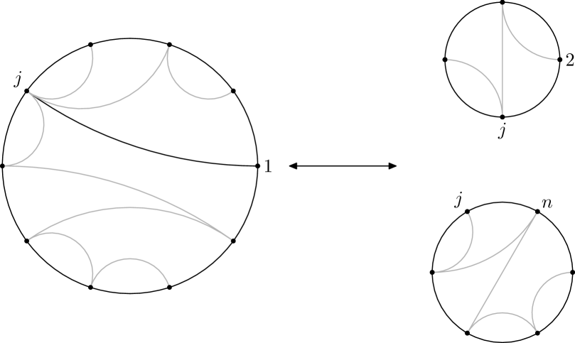
To count , remark that every nc tree that satisfies must have one and only one edge coming out of . Let be the other end of . We get two subtrees with the vertices to and with the vertices to . Each must be a noncrossing tree of order that has no edge that reaches , so is a -nc trees.
Conversely, for , suppose we’re given two nc trees and of order and that satisfy . Take the disk with evenly spaced vertices labelled from to on it’s boundary and draw the edge . We can reconstruct a nc-tree of order by inserting above the edge and under (see Figure 5). The resulting nc tree must satisfy , hence is of the type we were looking for.
Since there are such , this gives
∎
Lemma 3.4.
The numbers satisfy and
| (3) |
for .
Let be a finite embedded graph. For every connected component of , we define as the middle point of if the latter is non empty and as any point in if . We say that two connected components are adjacent if their closure intersect in a whole edge of .
Definition 3.5.
Let be a noncrossing tree. Using the same notation as above, we define it’s dual graph as the graph on the vertices and edges joining and if and are adjacent.
Proof.
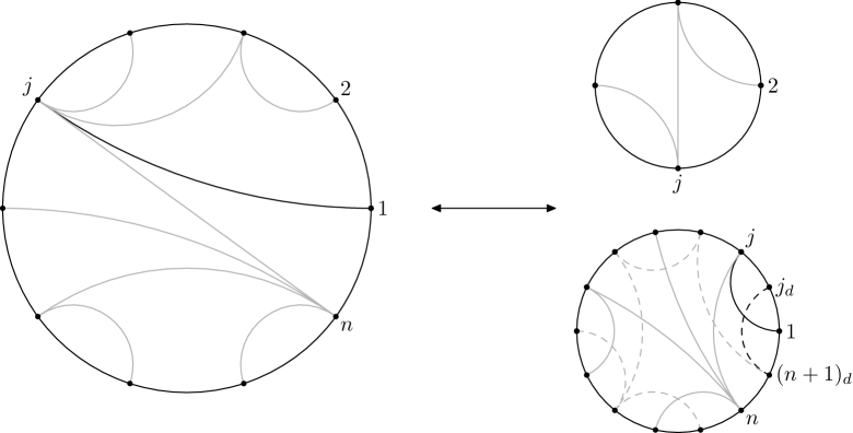
(of Lemma 3.4) For each , we want to count the number of nc trees such that is not an edge for all , but is an edge. This partitions the set of -nc trees in disjoint subsets (indexed by ). Hence, we only need to count the number of nc trees in each of those subsets.
Given a vertex such that is an edge, if is not an edge for all , then we can divide the nc tree into , the subgraph induced by vertices to and , the one induced by vertices to , so that and . Then is a -nc tree and is a -nc tree such that is an edge (see Figure 6).
The number of is . To count the number of -nc tree that have as an edge, consider the dual tree . Label its vertices by to counter clockwise, starting with the vertex between and (i.e. is at position , where ). Then, to ask for to be an edge in is equivalent to ask to be a -nc tree with . Hence, there are possibilities for the tree . This gives Equation (3). ∎
Theorem 3.6.
The numbers of -nc trees satisfy
| (4) |
for , where is the number of vertices.
Proof.
For , let . We have
Then if is the generating function, the recurrence relation gives . Using Lagrange’s inversion formula then gives us that from which the proposition follows. This is done in [Noy98]. ∎
This number is well known, see for instance [Knu97], and correspond to the sequence A001764 up to a reindexing. Those numbers also count ternary trees, a fact that we will use in Section 6.1.
We will see in Section 5 (see Remark 5.2) that counts the number of generic strata in the parameter space for generic anti-polynomial vector fields of degree . By generic stratum, we mean an open connected set in the parameter space for which each vector field is orbitally topologically equivalent to one another.
We are now interested in , the number of -nc-trees modulo rotations. We can obtain a formula for in terms of , so we begin with .
Proposition 3.7.
The numbers satisfy and
| (5) |
Proof.
This is done by expressing in a convolution of some and then using Lagrange’s inversion formula (see [Noy98]). ∎
Looking at some examples shows us that some nc-crossing tree may be obtained from others by rotation. The goal of the following discussion is to compute the number of nc trees modulo rotation.
Lemma 3.8.
Let be a -nc tree, then has a non-trivial rotational symmetry only if is even. Then, if this is the case, necessarily fixes one and only one edge with antipodal endpoints.
Proof.
Suppose acts on by rotation (i.e. it translates every vertex by a constant amount ( mod )). Index every vertex by to (mod ). Let . Then we have . We first claim that there exists some subgraph of such that . Indeed, let and let . Define as the subgraph induced by the edges that have an endpoint in . Then satisfy the claim.
If is an edge, we say that is internal if both its endpoints are in and external if it has only one endpoint in . Denote by the number of external edges of and by the number of internal edges of . Counting the edges over each , internal edges are counted only once, but external edges end up in two different graphs and . Hence, the total number of edges in is
| (6) |
This gives that . Hence we must have that , but since is not trivial, we must have that , thus is even and has order 2.
Now, suppose that is a rotational symmetry of and let be the subgraph as described above. Remark that there must be an external edge since, otherwise, we would have that , contradicting the parity of .
Let be the projection and lift to . Let be an external edge. Conjugating by a rotation, we may assume that is a lift of , with . Recall that the rotation lifts to a translation by . Consider the edge . Then, whenever , the edge and cross in , so we must have that , meaning that is an edge that fixes antipodal points. ∎
Theorem 3.9.
Denote by the number of -nc trees modulo rotation. We have that
| (7) |
This is sequence A296532 in the OEIS. This result was probably already proved, but we could not find a reference. Therefore, we added a proof here. A discussion about similar cases may be found in [Noy98].
Proof.
In the case is odd, proposition 3.8 tells us that there are precisely elements in every rotation class.
When is even, every nc tree that has a rotational symmetry has elements in it’s rotation class. So, we need to compute the number of nc trees that have a rotational symmetry to artificially add them up before dividing by .
Index vertices of by (i.e. vertex corresponds to ).
By proposition 3.8, counting those amounts to first counting nc trees that have as an edge and have a rotational symmetry.
Let be a nc tree on vertices that is invariant under the order rotation and the edge fixed by . Since splits in two -nc trees and and that those two trees mutually determine the other one via , we’re left to compute the number of -nc trees that have as an edge. By the same argument as in Lemma 3.4, going to the dual tree tells us that this number is . ∎
3.2. Characterization of the topological phase portrait with noncrossing trees
Definition 3.10.
Given a polynomial , the combinatorial invariant of is the -nc tree induced by the separatrix graph.
Theorem 3.11.
Let . If and have the same combinatorial invariant, then they are quasi-conformally equivalent. (In other words, there exists a quasi-conformal mapping that maps orbits of on orbits of ). In particular, the two vector fields are topologically orbitally equivalent.
Proof.
Let where is the separatrix graph. Since and have the same combinatorial invariant, there is a correspondence between the connected components of and of . Each is adjacent to either one or two singular points. In the first case, we denote it by and in the second case, by and . When there are two singular points, we label them so that .
Define . Then the pushforward of by gives
a real scaling of the horizontal vector field .
If is a sepal zone, this gives a conformal equivalence between and an infinite open strip which we denote . If is a petal zone, then maps it conformally to a half-plane that we denote by . In any case, extends to the adjacent separatrices, giving a homeomorphism from onto or .
If is a petal zone that corresponds to , define as identity map. If and are sepal zones, let , so that . We define
Recall that the rectifying coordinate maps orbits to horizontal lines. Since the ’s we’ve just built map horizontal lines to horizontal lines, the composition maps orbits to orbits.
Denote by the Beltrami coefficient of . One can compute that and the condition is seen to be equivalent to which is true. Note that all ’s are invertible and extend to homeomorphisms between and , where is either a strip or a half-plane. Hence, we have the following picture for every .
Now, the maps coincide along the closure of and (if ever) so we can glue them in a global homeomorphism that maps orbits to orbits. ∎
Let be a rotation of order . It acts on -noncrossing trees by rotating them when seen as embedded in . A direct consequence of the the preceding theorem is the following.
Corollary 3.12.
Suppose that has combinatorial invariant for . If there exists a rotation such that , then is topologically orbitally equivalent to .
4. Analytic invariant
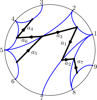
The analytic invariants of both and will be given in terms of . Indeed, this corresponds to both the complex time of and the circulation and the flux of . We will define below the invariant as integrals across the sepal zones, so we will establish an order on the zones that depends only on the combinatorial invariant.
Definition 4.1.
Let and let be its -nc tree. We define the -th vertex to be at position on the circle. To lighten the notation, we will write instead of .
-
(1)
We define a partial order on the edges. We say if , or . In other words, the edges attached to are ordered starting from and going around the circle in the positive direction.
- (2)
The way we choose to order the sepal zones is not intrinsically important for our study. However, we must choose one to go forward.
Definition 4.2 (Analytic invariant).
Let , be the combinatorial invariant and be the line segments defined in Definition 4.1 using . The analytic invariant of and is a vector , where .
Remark 4.3.
In the definition, we assumed that . This is indeed the case because of the choice of orientation of the ’s. We may suppose that is contained in its sepal zone and make a constant angle in with the vector field. In other words, the canonical normal vector of in the rectifying coordinate will make a constant angle in with the flow, so that the flux of across will be positive, and this is precisely the imaginary part of .
The following result proves that the analytic invariant is indeed invariant and, together with the combinatorial invariant, it describes the whole dynamics.
Theorem 4.4.
Let and be two monic centred polynomials of degree . If the two vector fields and are generic and have the same combinatorial and analytic invariants, then they are equal.
Proof.
We obtain a mapping such that using the same construction as in the proof of Theorem 3.11, but now the mappings between the horizontal strips in the rectifying coordinates are replaced with the identity, since the analytic invariants are the same (i.e. the corresponding strips are equal). The rectifying coordinates and the identity are holomorphic and extend to the separatrices continuously, which defines as holomorphic bijection.
A conformal mapping of on itself must be affine, and since the vector fields have the same combinatorial invariant, no rotation is allowed. Furthermore, both polynomials are centred, thus no translation is allowed. It follows that and . ∎
Recall that a permutation acts on -nc trees by a rotation of the vertices (mod ) and of the edges. Such a rotation will also change the order the analytic invariance by translating the indices (mod ).
Corollary 4.5.
Suppose has invariants for . If there exists a rotation that acts on so that and , then we have , that is, with ,
Proof.
If a rotation acts on , then it must be a rotation of order , therefore is a monic centred polynomial vector field. Its invariants are precisely and , so that it must be equal to . ∎
5. Realization
This is the main result of this section.
Theorem 5.1 (Realization).
Let . For every pair , where is a -noncrossing tree and , there exists a unique monic centred polynomial such that has for its invariant. Moreover, is also the unique monic centred polynomial such that has for its invariant.
Remark 5.2.
Let . The moduli space of the generic vector fields of is then , an open set with connected components (see Equation (4)). We call those components the generic strata. Each generic stratum of the parameter space can be analytically parametrized by .
We can quotient by the relation defined by if and only if there exists a rotation of order such that .
With a rotation of order , we can normalize a vector field by asking that . We can choose the invariants of this vector field as a representative of the class of .
Corollary 5.3.
Let be the set of vector fields such that has degree , is monic centred and normalized with . Then the moduli space of those generic vector fields is . It has connected component, where is given by Equation (7).
The proof of the theorem is similar to the realization construction found in [DES05] for a generic vector field . The combinatorial data and the analytic invariant allow us to construct a Riemann surface with open sets of in such a way that the vector field is well-defined on , where is a finite set. Then it is proved that has the conformal type of the Riemann sphere and the push-forward of will be for some polynomial , after perhaps applying a Möbius transformation. To obtain is a bit more tricky, since the push-forward of an antiholomorphic vector field is not, in general, antiholomorphic. The trick is to push-forward a well-chosen log-harmonic function: if is the appropriate isomorphism, then we will have .
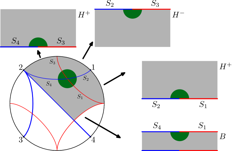
5.1. Construction of the Riemann surface
Consider a -nc tree and a vector . Recall that the dual is also a -nc tree. If we embed both and in the same closed disk so that the -th vertex of is mapped to and the -th vertex of , on , where , they divide the open disk in connected and simply connected components, provided the embedding is chosen so that two edges intersect at most once. We will call the intersection of two edges a singular point, which divides those edges in fours arcs that we will call the separatrices. By Proposition 2.7, there are components adjacent to only one singular point, which we call the petal zones, and components adjacent to two singular points, the sepal zones.
A petal zone in can be mapped by a homeomorphism to or , which we can choose so that it extends to the boundary as to map the singular point to ; of course, the separatrices must map on on each side of .
The sepal zones are ordered by from 1 to . The -th sepal zone can be mapped by a homeomorphism to a horizontal strip of width , which we can choose in a way that it extends to the boundary so as to map the singular points, say and , on and . There are two orientations for this; to choose the correct one, note that a sepal zone has an end on a vertex of and the other end on a vertex of . We choose a homeomorphism that maps a horizontal line in the strip oriented from left to right to a curve in from to . Then the four separatrices in are forced to be mapped on horizontal lines on each side of and in the strip.
We start constructing by sewing the half-planes and horizontal strips along a part of their boundary if and only if the image of this boundary in is the separatrix in . At this point, has the topological type of . The important point is that the vector field is well-defined on . The following discussion explains how to plug the holes at singular points and define a chart at .
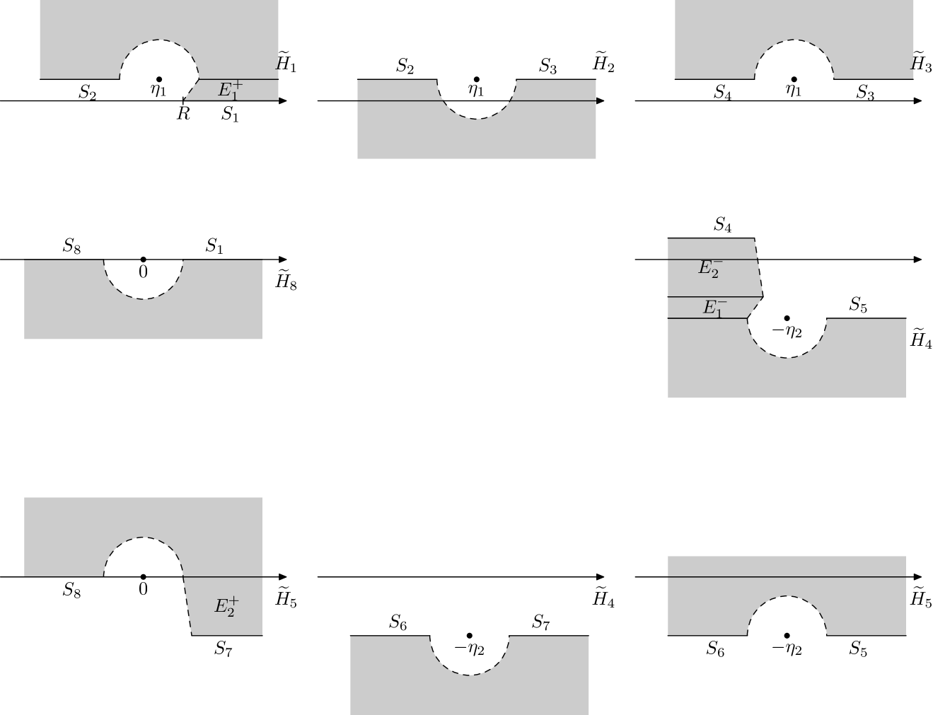
Neighbourhood of a singular point
Let be a singular point and the four separatrices attached to it, with an outgoing separatrix (any one of the two) and going anti-clockwise around . Then appears on the upper boundary of two charts, and lower boundary of two charts. For , we define as a upper (for odd) or lower (for even) half-disk from to (with ) with small enough radius centred at and contained in the chart. If we glue the ’s along the separatrices, we obtain a neighbourhood of . Let
This defines an isomorphism for some . We can extend to and obtain a chart of . See Figure 8. We can verify that , so that the dynamics is that of a simple saddle node.
Doing this at every singular point extends to a Riemann surface homeomorphic to .
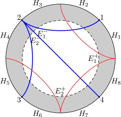
Neighbourdhood of infinity
To determine a conformal equivalence of a neighbourhood of infinity on to a neighbourhood in is more delicate than the previous paragraph. Indeed, the expected dynamics is one of a parabolic point and there are no canonical separatrices to divide the neighbourhood for us in . A neighbourhood of infinity will be defined to be any open set of that contains an annulus when seen in . See Figure 9(a). On the topological level, this correspond to quotienting to a single point. We now want to define a holomorphic chart on such a neighbourhood of infinity.
We will label vertices of by , with the -th vertex positioned at . Let be a neighbourhood of infinity. For a strip , has two components that we call ends. Let (resp. ) the end that lies at the -th (resp. -th) vertex. See Figure 9(a).
Starting with the petal zone between the vertices and , we glue the positive ends at (if any) to and we translate by the the analytic invariant of each of those ends. We obtain an open set of . We define by , with .
For the next petal zone (between and ), we glue negative ends at (if any) to and we translate by the analytic invariant of the positive ends at and by minus the analytic invariant of negative ends at 1 to obtain an open set . We then define by with .
We define and for every petal zones. See Figure 9(b). This defines a conformal map on that sends on some punctured neighboorhood of . We can then add to and extends as a holomorphic chart of on .
Equivalence with the Riemann sphere
Let be the Riemann surface obtained from after adding the singular points and . It is a compact manifold with no boundary. We can compute the Euler characteristic with the following triangulation: the vertices are the singular points and , the edges are the separatrices, and the faces are the half-planes and the strips. We have vertices, edges and faces, so that . Therefore, is a topological sphere and thus, by Riemann’s Uniformization Theorem, it has the conformal type of the Riemann’s sphere .
5.2. Proof of the Realization Theorem
We now prove Theorem 5.1.
Let be a conformal mapping. Since we can post-compose by a Möbius transformation, we can suppose that . We can further normalize by requiring that in the chart has the form . Note that is still not unique, as we can post-compost by an affine transformation , where is a -root of unity. To fix the rotation, we require that the real interval , for large enough, on be mapped by in the attracting sector at infinity that intersect .
The vector field is well-defined on . Let be obtained from . In a chart of a marked point , the vector field becomes a simple saddle node, so that can be extended on as a meromorphic function with a simple pole. In a chart of , becomes a parabolic point of codimension (multiplicity ). Therefore, we can extend at infinity by . Since is a meromorphic function of with a single zero of order at infinity, it must be of the form , where is a polynomial of degree . We can centre with a translation, and it must be monic since in the coordinate , has the form for small, since and .
To realize , we consider the vector field on . A simple calculation shows that , and since , it follows that on and can be extended on .
6. Anti-polynomial vector fields with maximal number of heteroclinic connections
Given a fixed -noncrossing tree, consider the family of structurally stable vector field in the generic stratum parametrized by the analytic invariant . When , the corresponding sepal zone collapses to a curve. Indeed, in the rectifying coordinate, is the width of the horizontal strip. If , then this curve contains a heteroclinic connection and . If , then the two simple singular points on the boundary of the sepal zone coalesce into a double saddle point. In both cases, the initial noncrossing tree is no longer adequate to describe the topology of the phase portrait.
The bifurcation occuring in are of the following type.
-
(1)
Bifurcation of a heteroclinic connection. Under pertubation in the right direction, the heteroclinic connection breaks and gives rise to a sepal zone.
-
(2)
Bifurcation of a multiple saddle point. Under perturbation in the right direction, a multiple points breaks in singular points of smaller codimension and gives rise to at least one sepal zone.
-
(3)
Intersection of the former two types.
Note that it is impossible to find a closed loop made of orbits, it would necessarily contain a non-saddle singular point.
6.1. Case of heteroclinic connections
This case can only happen when every singular point is simple. Indeed, the graph formed by the singular points as vertices and heteroclinic connections as edges must be a tree, and a tree with edges must have vertices. Since there are heteroclinic connections, there remains exactly outgoing and incoming separatrices. Since each marked point at infinity must attach to at least one separatrix and there are marked points, there is exactly one separatrix attached to each marked point.
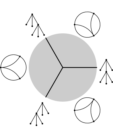
The topological invariant of this case has a beautiful simplicity: the separatrix graph, made of the union of heteroclinic connections, (outgoing and incoming) separatrices, and singular points, can be extended to a ternary tree by adding marked point at infinity as vertices. By ternary tree, we mean an ordered rooted tree for which each vertex is either a leaf or has three children. The root of the tree is the singular point attached to the outgoing separatrix tangent to and identified with that marked point (so that the tree has vertices and vertices).
We say that a vertex is an internal vertex if it has children. We say that an edge is an internal edge if it is connected to two internal vertices. We define the following total order on the internal edges: we say that if either a path from the root to must first pass (see e.g. edges on Figure 10), or a direct path from the root to is further to right than a direct path from the root to (see e.g. edges or on Figure 10).

Theorem 6.1.
-
•
(Topological invariant) To every anti-polynomial vector field with heteroclinic connections, we can associate a unique ternary tree with internal vertices made with the singular points, the incoming and outgoing separatrices, the heteroclinic connections, and the marked points at infinity. The root of the tree is the singular point attached to outgoing separatrix tangent to .
-
•
(Analytic invariants) To every anti-polynomial vector field with heteroclinic connections, we can associate a unique vector , where each component is the integral of over an heteroclinic connection and the order is given by the ternary tree.
-
•
(Equivalence) Two such vector fields with the same topological invariant are quasi-conformally (and hence orbitally topologically) equivalent. Furthermore, if they also have the same analytic invariant, then they are equal.
-
•
(Realization) To every pair , where is a ternary tree with interior vertices and , there exists a unique monic centred polynimial such that has heteroclinic connections and has as invariants.
Corollary 6.2.
Let be the set of anti-polynomial vector fields of degree with heteroclinic connections. Then has equivalence classes, where is the topological orbital equivalence of vector fields.
Proof.
By Theorem 6.1, there are as many equivalence classes of as there are rooted ternary trees with internal vertices.
In Section 3.1, we noted that that those numbers are the same than the numbers we obtained for generic anti-holomorphic polynomial vector fields. Indeed, it is well known that the number of ternary tree with internal edges is . ∎
Proof of Theorem 6.1.
The idea of the proof is the same as the Realization Theorem 5.1: we construct a Riemann surface isomorphic to with half-planes and push the vector field from the surface to . This case is even simpler, since there are no horizontal strips, only half-planes. The heteroclinic connections will corresponds to intervals on the boundary of of the half-planes.
First, we want to embed the ternary tree in . We start by adding a vertex over the root and attaching it to the root with an edge; this corresponds to the marked point that was identified with the singular point. Now, we order the leafs from left to right, i.e. leaf 1 is the first leaf reached by a depth-first search in the tree by always going left, leaf 2 is the second leaf reached, and so on, and the added vertex over the root is leaf 0. Then we embed the tree in by mapping the -th leaf on on , and the internal vertices to points in so that the edges can be mapped to simple curve that do not cross each other. See Figure 11.


Now, the embedded ternary tree divides in simply connected domains. Each component is adjacent to a segment of ; let be the component adjacent to and , the one adjacent to , for . A component is topologically equivalent to , by abuse of notation, we will use for the half-plane; a chart of the Riemann surface will be of the form , where is the injection . Notice that the vector field is well-defined on every half-plane .
Each (resp. ) in is adjacent to two edges and, say, internal edges. Suppose are the internal edges. Then we mark with , by , , by , and lastly by (resp. ). We mark and by the corresponding vertices of the tree.
We are now ready to construct the Riemann surface. Let be the Riemann surface obtained by sewing a marked interval of with the corresponding marked interval on another . Equivalently, this can be seen in , where will share an edge with . We can add the marked points to the same way we did in Section 5.1. We also add a point at infinity the same way we did in that section, except that are no ends and translations.
The end of the proof is identical to proof in Section 5.2: a well-chosen conformal mapping will push to , with a monic centred polynomial of degree . Moreover, pushes to . The phase portrait of must have heteroclinic connections by construction, and its invariants must be . ∎
6.2. Bifurcation diagram for quadratic anti-polynomial vector fields
As a simple application of the classification of generic anti-polynomial vector fields and anti-polynomial vectors with a maximal number of heteroclinic connection, we can describe the complete bifurcation diagram of the family , with . The only possible non-structurally stable objects are a double saddle point, which only occur when , and a heteroclinic connection, which happens if and only if is real, where are the roots of .
A simple calculation shows that
This is in if and only if and , . The parameter space is divided by three rays , and , , and each open component outside the rays is a generic stratum.
Starting with , the phase portrait has a heteroclinic connection oriented from to (since ) on the real interval and the phase portrait is symmetric with respect to . When inscreases in the interval , the singular point rotate counter-clocktwise around 0 until it reaches . At , there is again a heteroclinic connection oriented from to (since ).
When decreases from 0 to , the singular point rotates clockwise around 0 until it reaches at . At , the phase portrait has a heteroclinic connection oriented from to (since ).
References
- [Bad20] Peter J Baddoo. Lightning solvers for potential flows. Fluids, 5(4):227, 2020.
- [BD10] Bodil Branner and Kealey Dias. Classification of complex polynomial vector fields in one complex variable. Journal of Difference Equations and Applications, 16(5-6):463–517, 2010.
- [CKM+17] Ulrike Cordes, G. Kampers, T. Meißner, C. Tropea, J. Peinke, and M. Hölling. Note on the limitations of the theodorsen and sears functions. Journal of Fluid Mechanics, 811:R1, 2017.
- [DES05] A. Douady, F. Estrada, and P. Sentenac. Champs de vecteurs polynomiaux sur . unpublished, 2005.
- [GR25] Jonathan Godin and Christiane Rousseau. Generic complex polynomial vector fields with real coefficients. Qual. Theory Dyn. Syst., 24:68, 2025.
- [Ily08] Yakovenko Ilyashenko. Lectures on analytic differential equations, volume 86. American Mathematical Soc., 2008.
- [Knu97] D.E. Knuth. The Art of Computer Programming: Fundamental Algorithms, Volume 1. Pearson Education, 1997.
- [Noy98] Marc Noy. Enumeration of noncrossing trees on a circle. Discrete Mathematics, 180(1-3):301–313, 1998.
- [Tre24] Lloyd N Trefethen. Polynomial and rational convergence rates for laplace problems on planar domains. Proceedings of the Royal Society A, 480(2295):20240178, 2024.
- [VD75] Milton Van Dyke. Perturbation methods in fluid mechanics/annotated edition. NASA STI/Recon Technical Report A, 75:46926, 1975.