Graph Attention Networks Unleashed: A Fast and Explainable Vulnerability Assessment Framework for Microgrids

Abstract

Independent microgrids are crucial for supplying electricity by combining distributed energy resources and loads in scenarios like isolated islands and field combat. Fast and accurate assessments of microgrid vulnerability against intentional attacks or natural disasters are essential for effective risk prevention and design optimization. However, conventional Monte Carlo simulation (MCS) methods are computationally expensive and time-consuming, while existing machine learning-based approaches often lack accuracy and explainability. To address these challenges, this study proposes a fast and explainable vulnerability assessment framework that integrates MCS with a graph attention network enhanced by self-attention pooling (GAT-S). MCS generates training data, while the GAT-S model learns the structural and electrical characteristics of the microgrid and further assesses its vulnerability intelligently. The GAT-S improves explainability and computational efficiency by dynamically assigning attention weights to critical nodes. Comprehensive experimental evaluations across various microgrid configurations demonstrate that the proposed framework provides accurate vulnerability assessments, achieving a mean squared error as low as 0.001, real-time responsiveness within 1 second, and delivering explainable results.

I Introduction

An independent microgrid, like a battlefield or island microgrid, operates separately from the main grid, supplying electricity to a localized area by integrating distributed energy resources and loads via interconnected buses, transformers, and lines. Assessing the vulnerability of independent microgrids is essential to ensure its normal power supply capacity against disruptions, particularly in scenarios like deliberate attacks and natural disasters. On the other hand, when constructing a new microgrid or designing a reconfiguration plan, rapid vulnerability assessments are necessary to support iterative optimization processes. Therefore, developing a fast, accurate, and explainable method for assessing the microgrid vulnerability is important for enhancing the robustness and anti-destructiveness of independent microgrids in both civilian and military applications.

In recent years, numerous studies have investigated power systems in terms of reliability, resiliency, and vulnerability [1, 2, 3]. These indices differ in focus: reliability represents the system’s ability to deliver uninterrupted power under normal conditions; resiliency measures the system’s capacity to recover and maintain functionality after disruptions; and vulnerability assesses the system’s susceptibility to failures or attacks. Reliability and resiliency are widely studied in power systems, yet vulnerability analysis has not been widely emphasized though it is particularly worth studying in extreme and battlefield scenarios [4]. In this study, we focus on the load-securing capability post-disruption in battlefield conditions of the independent microgrids, using the expected load shedding rate (ELSR) after disruptions as the vulnerability evaluation indicator. Let $L$ be the total load demand of the microgrid, $N_{a}$ the total number of simulated attack scenarios, and $U_{i}$ the unsatisfied load after the $i$-th attack, the vulnerability indicator $V$ is then defined as follows:

$$V=\lim_{N_{a}\to\infty}\frac{1}{N_{a}}\sum_{i=1}^{N_{a}}\frac{U_{i}}{L}.$$ (1)

Since it is impossible to model all potential environmental actions (i.e., $N_{a}\to\infty$), Monte Carlo simulation (MCS) is widely used for estimating such a dynamic indicator [5, 6, 7]. Taking the estimation of the ELSR indicator as an example, MCS first generates numerous attack scenarios for the microgrid and recalculates the power flow for each post-disruption microgrid. The ELSR value can be obtained by averaging the load shedding rates across all scenarios. While effective in handling diverse data distributions and producing probabilistic outputs, MCS is computationally intensive, making it unsuitable for real-time applications in fast-changing environments. This limitation also restricts MCS-based methods in related optimization issues, where iterative evaluations of computationally expensive objective functions can lead to prohibitive resource and time demands.

With recent advancements in artificial intelligence, machine learning (ML)-based methods have achieved significant success in evaluating computationally costly indicators [8, 9]. By effectively approximating complex and high-dimensional functions, ML-based models substantially reduce the computational burden of assessing expensive metrics. Once trained, these models enable rapid calculation with near-instant predictions, making them ideal for real-time applications in dynamic environments like power systems. Some studies have integrated ML-based methods with MCS to accelerate assessment [10, 11, 12, 13], while others have directly applied ML for evaluating system vulnerability or reliability [14, 15, 16]. However, several prominent challenges still remain: (1) vulnerability assessments are comparatively underexplored, with reliability receiving more research attention; (2)the complex network structure of microgrids is often neglected, with models focusing primarily on isolated bus features; (3) extensive labeled data across diverse disruptions is required, but such data is limited and obtain-expensive; and (4) model explainability is rarely considered, making many ML models difficult to trust as they function as black boxes.

To address these challenges, we propose a novel and local explainable ML-based vulnerability assessment framework through a graph attention network with self-attention pooling (GAT-S) for assessing independent microgrid vulnerability rapidly. MCS is first used to generate labels for training and test data, which involves steps including microgrid initialization, probabilistic attack simulation, isolation division, and optimal flow calculation. Data resampling and feature selection techniques are applied to improve the data quality. The proposed neural network GAT-S is constructed by two graph attention (GAT) convolutional layers for node-level information integration, a self-attention pooling layer for explainable graph-level aggregation, and a fully connected layer for final prediction. Taking the bus and line features of the initialized microgrids as inputs and the MCS-derived ELSR values as labels, the GAT-S is trained offline through supervised learning. Once trained, the GAT-S model can immediately assess the microgrid vulnerability for any given scenario, offering both computational efficiency and adaptability to dynamic conditions. The learned attention weights meanwhile reveal a local explainability of how every bus contributes to the graph-level vulnerability. Computational experiments on 33, 66, and 100-bus instances demonstrate the proposed method’s effectiveness and advantages over other ML-based approaches, achieving a mean squared error (MSE) as low as 0.001. Further experiments also show the model’s explainability and generalization ability. The main contributions of our work can be summarized as follows:

• A novel fast ML-based vulnerability assessment framework for independent microgrids is proposed, integrating Monte Carlo simulation with an advanced neural network, enabling fast, accurate, and explainable vulnerability evaluations.

• A workflow for generating data labels through MCS is proposed, incorporating scene-wide probability attacks, post-disruption optimal power flow calculations, and data preprocessing to ensure efficient and effective data generation within a limited timeframe.

• A local explainable neural network, GAT-S, is proposed for vulnerability assessment, integrating graph attention networks and a self-attention pooling mechanism to enhance feature data fusion at both the node and graph levels and improve model explainability.

The rest of this study is structured as follows: Section II reviews the related work concerning the vulnerability indicators and the assessment methods. Section III elaborates the proposed vulnerability assessment framework, including the MCS-based data generation approach, data preprocessing techniques, and the GAT-S neural network. Section IV conducts extensive experiments and discussions on both the model explainability, effectiveness, and generalization ability. Section V finally concludes this study and identifies several future directions.

II Related Work

II-A Definitions of Vulnerability Indicators

Power system vulnerability lacks a fixed quantitative definition due to varying practical needs. Different studies focus on different aspects, including node-level, edge-level, and system-level vulnerabilities. Node-level vulnerability metrics identify critical nodes whose failure may undermine stability [17, 18], while edge-level vulnerability metrics focus on key connections and their impact on network robustness [19, 20]. In contrast, system-level vulnerability metrics offer comprehensive perspective by considering cumulative effects and interactions among components [21].

In another way of categorization, vulnerability can be categorized into three main types: structural, state, and integrated. Structural vulnerability examines the system’s topology, focusing on how node and link configurations affect robustness against failures. Some researchers use complex network theory to define structural vulnerability through metrics like network centrality [22], though this approach overlooks the importance of electrical characteristics. State vulnerability, on the other hand, considers the network’s dynamic operational conditions, such as load and stability. For instance, Fang et al. [19] incorporated power flow into structural metrics, while Shen et al. [23] developed an early fault warning system based on dynamic power flow to assess reliability. Integrated vulnerability combines structural and state factors, providing a comprehensive evaluation by considering both topology and real-time operational conditions, as demonstrated in [24, 25].

In this study, driven by the practical need to ensure power supply for critical loads, we define the vulnerability indicator as the expected load shedding rate, as formulated in (1). This indicator serves as a system-level and integrated metric that is widely used to quantify load deficits resulting from network disruptions.

II-B Methods for Energy System Assessment

Simulation-based and analytical methods are the two primary approaches for assessing power system vulnerability and reliability [26]. Analytical methods [27, 28, 29, 30], which focus on static and structural indicators, are unsuitable for the disruption-conditioned assessment indicators used in this study. Among simulation-based methods, MCS is prominent. Gautam et al. [21] used a non-sequential MCS framework to evaluate the resilience of active distribution systems by integrating a probabilistic extreme event model, impact assessment model, and optimal restoration model. He et al. [31] applied MCS to estimate the system average interruption duration index (SAIDI) and the expected energy not supplied (EENS) for cyber-physical distribution systems. Similar studies can also be found in [5, 6, 7].

Due to the time-consuming nature of the simulation processe, many studies have proposed approaches to accelerate MCS. Da et al. [32] combined the cross-entropy method with MCS to calculate distribution network risk indices (e.g., overload probabilities), achieving assessments on networks of 14, 24, and 118 nodes in 4 to 57 minutes. Nikmehr et al. [33] developed a quantum computing model to speed up MCS-based power system reliability assessments. Moreover, ML methods have also been widely integrated into MCS for faster calculations. Li et al. [10] incorporated an ML perception model into distribution network state assessments, combining it with sequential MCS for reliability evaluation. Stern et al. [11] used a support vector machine (SVM) to accelerate MCS for gas network failure probability estimation. Dehghani et al. [12] applied a Bayesian Additive Regression Tree (BART) to identify key training samples in MCS, demonstrating the robustness of the method. Lin et al. [13] employed a dynamic Bayesian belief network (DBBN) to model wind and solar energy output distributions based on historical data. Integrated with rolling-horizon unit commitment, the DBBN was embedded in a sequential MCS framework to evaluate reliability metrics through extensive random sampling of system states.

However, MCS-based assessment methods are often too time-consuming to be integrated into system planning optimization, which generally requires millions of objective evaluations. To address this, surrogate models have gained popularity as a computationally efficient alternative. However, their application to microgrid vulnerability assessment remains limited due to the complexity of power flow dynamics and interdependencies. Zhou et al. [14] demonstrated the feasibility of using a basic artificial neural network (ANN) to quickly determine power system dynamic security, employing heuristics to generate training data and testing it on the IEEE 50-generator system. More recently, Cao et al. [15] introduced a graph neural network (GNN) for reliability assessment in electricity-hydrogen systems, incorporating a feature selection method to enhance local explainability.

Despite showing great potential, existing ML-based methods face significant limitations: the design of existing neural networks fails to capture complex interdependencies and stochastic power flows in microgrids, and the limited explainability of most ML models undermines user confidence by obscuring how vulnerability predictions are made. Thus, developing an ML-based model with robust learning capabilities and high explainability is crucial for microgrid vulnerability assessment.

III Proposed Method

This study proposes to assess the independent microgrid vulnerability through a novel and local explainable ML-based framework, which includes four modules: MCS-based data generation, data preprocessing, model training, and vulnerability assessment, as detailed in Fig. 1. Data generation involves microgrid initialization, probabilistic attacks, isolation division, and optimal flow calculation, with each microgrid simulated $N_{a}$ times until the vulnerability indicator converges. Data resampling and feature selection techniques address data imbalance and enhance quality. The GAT-S model structure and its supervised learning method are detailed in the model training module. The pre-trained GAT-S can immediately output the predicted vulnerability value and the explainable node weights. A further illustration of these steps is provided in this section.

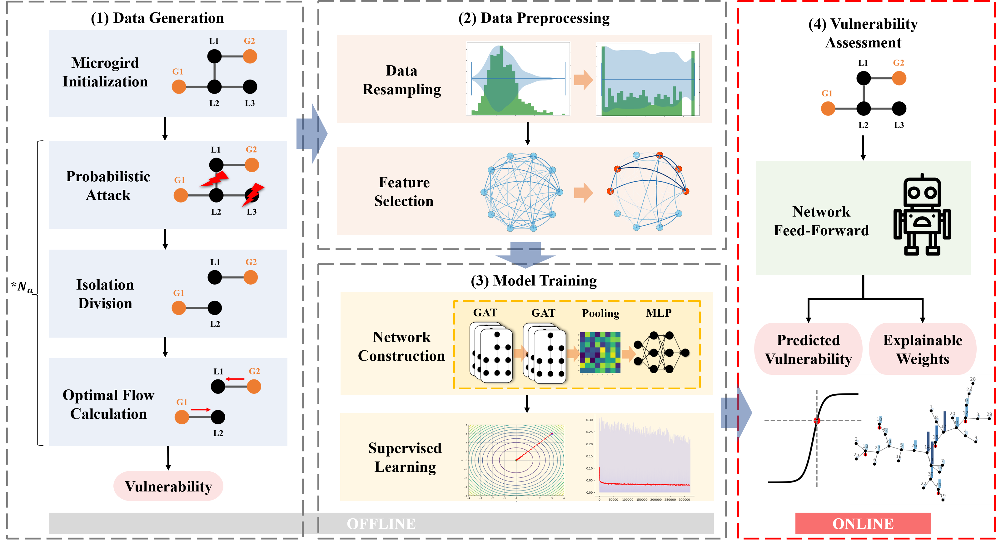
Figure 1: The proposed vulnerability assessment framework includes four modules: (a) Data Generation: Independent microgrids are initialized, and probabilistic attacks simulate disruptions to buses and lines, with isolation division and optimal flow calculations determining the expected load shedding rate to assess vulnerability. (b) Data Preprocessing: Resampling and feature selection enhance dataset quality and relevance. (c) Model Training: The GAT-S model is developed and trained using supervised learning. (d) Vulnerability Assessment: The pre-trained GAT-S model evaluates microgrid features to predict the vulnerability as well as node weights through a network feed-forward calculation.

III-A Monte Carlo Simulation for Data Generation

During model training, the vulnerabilities of various microgrids serve as label data, while the microgrids features are the inputs. Since real data accounting for the effects of external disruptions on microgrids is unavailable, MCS is used to simulate disruption scenarios. The label data (i.e., ELSR values) can then be calculated by analyzing the power flow of the post-disruption microgrids. The detail process for data generating will be introduced in this section in detail.

III-A1 Independent Microgrid Initialization

Bus and line properties are crucial for microgrid construction. Table I summarizes these properties and their parameters, which are either fixed or uniformly distributed. Each bus has loads, with generators randomly assigned to 15% of the buses. All generators have the same power capacity, collectively set at 120% of the total load to ensure power balance. All loads and generators are controllable in this study.

TABLE I: Properties and parameter settings for initialized independent microgrids.

	Property	Symbol	Value/Range	Unit
Bus	Voltage Magnitude	$V_{i}^{Mag}$	[0.95, 1.05]	p.u.
	Load Active Power Injection	$P_{i}^{load}$	[0.1, 0.5]	MW
	Load Reactive Power Injection	$Q_{i}^{load}$	[-10, 0]	MVar
	Generator Capacity	$P_{i}^{gen}$	$\frac{8}{N}\sum_{i=1}^{N}P_{i}^{load}$	MW
Line	Line Resistance	$R_{ij}$	[0.01, 1]	$\Omega$
	Line Reactance	$X_{ij}$	[0.01, 1]	$\Omega$
	Rated Current	$I_{rated}$	1	KA

Representing each independent microgrid as a graph $G=(B,E)$, where $B$ denotes the set of buses, and $E$ denotes the set of transmission lines, there are several constraints should be satisfied:

$$|E|=|B|-1,$$ (2)

$$P_{i}^{\text{gen}}-P_{i}^{\text{load}}=\sum_{j\in\mathcal{N}(i)}P_{ij},$$ (3)

$$Q_{i}^{\text{gen}}-Q_{i}^{\text{load}}=\sum_{j\in\mathcal{N}(i)}Q_{ij},$$ (4)

$$\frac{\sqrt{P_{ij}^{2}+Q_{ij}^{2}}}{{Vol}_{i}}\leq I_{ij}^{rated},\quad\forall(i,j)\in E,$$ (5)

where $P_{ij}$ and $Q_{ij}$ are respectively the active and reactive power flows on the lines. Among these equations, (2) enforces the radial topology constraint, preventing the formation of loops. (3) and (4) impose the power balance constraint, ensuring the total injected active and reactive power at each node equals the total power consumed. (5) sets the line’s maximum current limit.

To satisfy the radial topology constraint, microgrid lines are created using a randomized tree method: (1) select a root node; (2) randomly choose an existing node as the parent and connect a new node to it; (3) repeat this for $N-1$ times until all nodes are included in the tree.

III-A2 Probabilistic Attack Simulation

To assess microgrid vulnerability as defined in (1), various disruption scenarios are simulated. Unlike the fixed $N-k$ disruption pattern used in traditional studies [34], any bus or line may be disrupted based on assigned probabilities. Additionally, instead of assuming uniform disruption probabilities as in [35], these probabilities vary according to the network importance of each component. Specifically, the disruption probabilities for bus $i$ and line $e$ are calculated according to their normalized degree centrality $C_{d}(i)$ and normalized edge betweenness centrality $C_{b}(e)$, respectively, as defined below:

$$p(i)=p_{min}+(p_{max}-p_{min})\cdot C_{d}(i),$$ (6)

$$p(e)=p_{min}+(p_{max}-p_{min})\cdot C_{b}(e),$$ (7)

where $p_{min}$ and $p_{max}$ (respectively set as 0.01 and 0.2 in this study) represent the bounded minimum and maximum disruption probabilities. This formulation highlights that higher-value facilities are more vulnerable in conflict scenarios. In each attack scenario, buses and lines are probabilistically disrupted, requiring the simulation of $N_{a}=1000$ scenarios to calculate the ELSR indicator for each microgrid.

III-A3 Load Shedding Rate Calculation

After a disruption alters the microgrid’s topology, power resources must be re-dispatched to restore balance. The first step is isolation division, which involves identifying all connected components in the microgrid’s graph representation after disrupted buses and lines are marked. This can be done using graph traversal algorithms like depth-first search (DFS) or breadth-first search (BFS). Each connected component represents a section of the network that can operate independently.

After identifying the isolated components, the next step is to calculate the optimal power flow within each connected component by solving power flow equations to determine the optimal distribution of electrical power across the remaining buses and lines. Since various optimization techniques are well-established for this purpose [36, 37], this paper does not focus on them. To address the need to secure critical loads in a battlefield environment, the objective function is designed to maximize the load satisfaction rate.

The load-shedding rate after the attack is calculated as the ratio of the shedded load power to the load demand power. Following $N_{a}$ simulation iterations, the vulnerability indicator is determined using (1).

III-B Data Resampling and Feature Selection

The MCS-obtained data often shows significant imbalance, which restricts models from capturing data features in extreme scenarios. To address this, a probabilistic data resampling method is employed. The dataset is divided into discrete bins based on the label values, and sample counts within each bin are determined. Sampling weights are then calculated as the inverse of these counts, giving higher weight to underrepresented classes. After normalization, these weights produce sampling probabilities for each sample. Random sampling with replacement is performed using these probabilities, balancing the dataset and enhancing the model’s robustness and generalization capability.

In addition to the adjacency matrix, several bus and line features also serve as the model inputs, including the bus active power, bus reactive power, node type (i.e., generator or load), node degree, line resistance, and line reactance. Each of these features is standardized to accelerate the learning process.

III-C Graph Attention Network with Self-attention Pooling

The proposed GAT-S model consists of two GAT convolutional layers with residual connections and normalization, a self-attention pooling layer, and a fully connected layer, as illustrated in Fig. 2. The GAT convolutional layers leverage attention mechanisms to capture complex relationships between nodes and their neighbors, incorporating both node and edge features. Residual connections mitigate the vanishing gradient problem and improve training efficiency, while layer normalization stabilizes and accelerates convergence. The self-attention pooling mechanism dynamically aggregates node embeddings into a graph-level representation by assigning learnable importance weights to nodes, enhancing the model’s ability to capture global graph information. Finally, the fully connected layers transform the aggregated graph-level representation into the final output. These components collectively enable the model to process complex graph-structured data effectively.

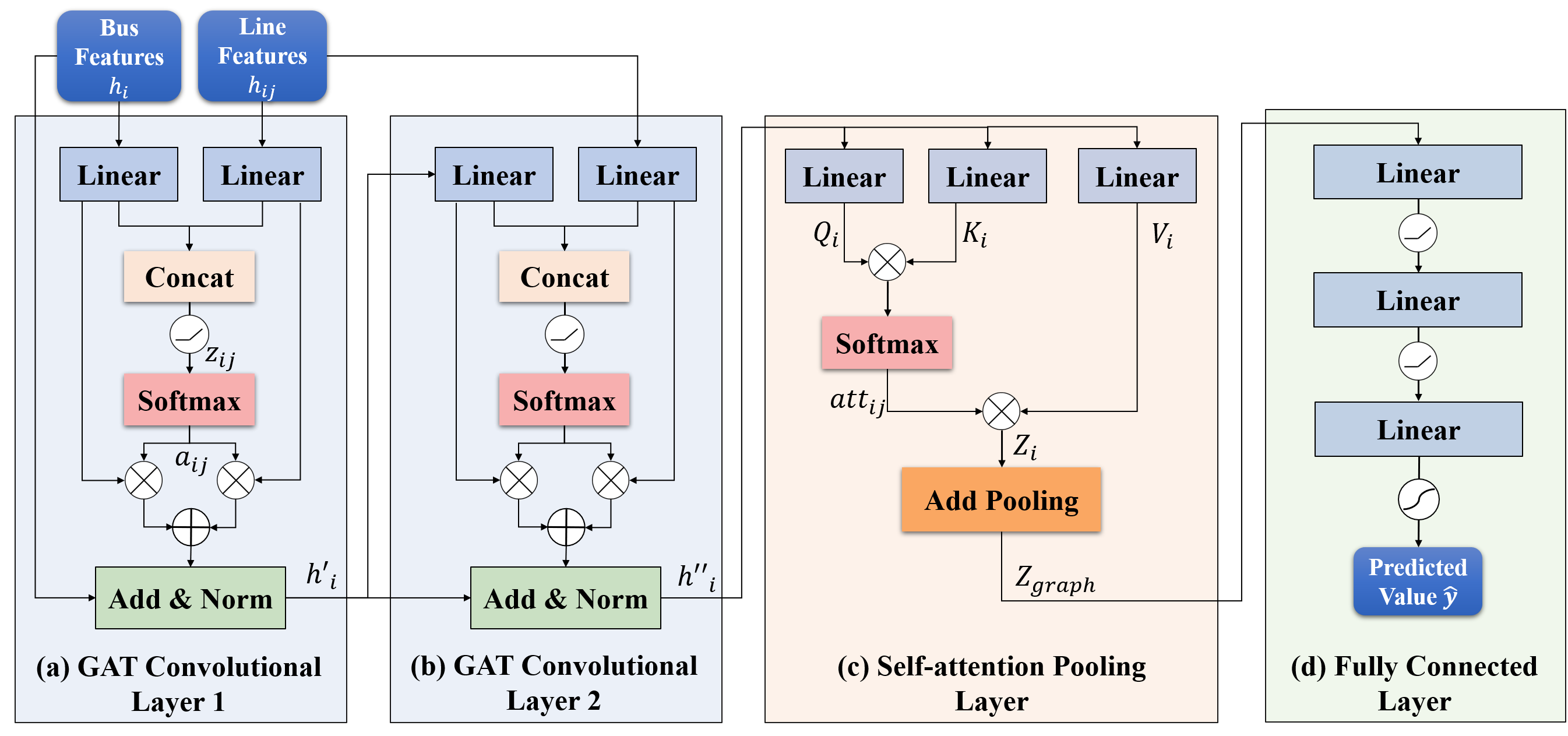
Figure 2: The structure of the proposed GAT-S neural network. Four layers are included: two GAT convolutional layers with residual connections and normalization, a self-attention pooling layer, and a fully connected layer. Taking the selected bus features, line features, and adjacency matrix as inputs, the GAT-S outputs the predicted microgrid vulnerability value.

The first GAT convolutional layer employs a multi-head attention mechanism to update node embeddings by aggregating information from neighboring nodes and edges. Specifically, for each node $i$, the updated embedding is computed as:

$$h^{\prime}_{i}=\sigma\left(\sum_{k=1}^{H}\sum_{j\in\mathcal{N}(i)}\alpha_{ij}^{k}W^{k}h_{j}+\sum_{k=1}^{H}\sum_{j\in\mathcal{N}(i)}\alpha_{ij}^{k}W_{e}^{k}h_{ij}\right),$$ (8)

where $H$ is the number of attention heads (set to $H=4$ in this study), $\sigma$ is the non-linear activation function (e.g., Relu), $h_{j}$ is the feature vector of the node $j$, $h_{ij}$ is the feature vector of edge $e_{ij}$, $W^{k}$ and $W_{e}^{k}$ are learnable weight matrices for the $k$-th attention head, $\alpha_{ij}^{k}$ is the attention coefficient for the $k$-th head, which determines the importance of node $j$ to node $i$.

The attention coefficient $\alpha_{ij}^{k}$ is computed as:

$$\alpha_{ij}^{k}=\frac{\exp(z_{ij}^{k})}{\sum_{l\in\mathcal{N}(i)}\exp(z_{il}^{k})},$$ (9)

where the attention score $z_{ij}^{k}$ is defined as:

$$z_{ij}^{k}=\text{Relu}\left(\mathbf{a}^{T}\cdot[W^{k}h_{i}\|W^{k}h_{j}\|W_{e}^{k}h_{ij}]\right).$$ (10)

Here, $\mathbf{a}$ is the attention weight vector, and $[\cdot\|\cdot]$ denotes concatenation. To improve training stability and prevent gradient vanishing, a residual connection is added, and layer normalization is applied:

$$h^{\prime}_{i}=\text{LayerNorm}\left(h^{\prime}_{i}+\text{ResidualFC}(h_{i})\right),$$ (11)

where ResidualFC is a linear transformation that adjusts the dimensionality of the input features to match the output of the GAT convolutional layer.

The second GAT convolutional layer refines the node embeddings from the first layer using a similar process, but with a single attention head ($H=1$). The updated node embeddings are denoted as $h^{\prime\prime}_{i}$. After that, a self-attention pooling mechanism aggregates the node embeddings into a graph-level representation. For each node $i$, the query, key, and value vectors are computed as:

$$\mathbf{Q}_{i}=\mathbf{W}_{q}h^{\prime\prime}_{i},\quad\mathbf{K}_{i}=\mathbf{W}_{k}h^{\prime\prime}_{i},\quad\mathbf{V}_{i}=\mathbf{W}_{v}h^{\prime\prime}_{i},$$ (12)

where $\mathbf{W}_{q}$, $\mathbf{W}_{k}$, and $\mathbf{W}_{v}$ are learnable weight matrices. The attention scores between nodes are computed as:

$$\text{att}_{ij}=\text{softmax}\left(\frac{\mathbf{Q}_{i}\cdot\mathbf{K}_{j}^{\top}}{\sqrt{d}}\right),$$ (13)

where $d$ is the dimensionality of the query and key vectors. The node embeddings are then aggregated as:

$$\mathbf{Z}_{i}=\sum_{j=1}^{N}\text{att}_{ij}\mathbf{V}_{j}.$$ (14)

The graph-level representation ${Z}_{\text{graph}}$ is obtained by averaging the aggregated node embeddings and can thus calculate the predicted vulnerability value $\hat{y}$ as below:

$$\mathbf{Z}_{\text{graph}}=\frac{1}{N}\sum_{i=1}^{N}\mathbf{Z}_{i}.$$ (15)

$$\hat{y}=\text{Sigmoid}\left(\mathbf{W}_{\text{fc}}\cdot\text{Relu}\left(\mathbf{W}_{\text{out}}\cdot\mathbf{Z}_{\text{graph}}+\mathbf{b}_{\text{out}}\right)+\mathbf{b}_{\text{fc}}\right)$$ (16)

IV Experiments and Results

Experiments were performed on a PC with an AMD Ryzen 7 5800H CPU @3.2 GHz and an RTX 3060 GPU. The source code for this study will soon be available open-source . This section conducts experiments and gives discussions sequentially on data generation, model training, model assessment, model explainability, model effectiveness, and model generalization ability.

IV-A Data Generation and Model Training

The experiments involve 33, 66, and 100-bus microgrids, with 1000 training and 100 test instances generated for each size, as stated in Section III-A. Parameter distributions align with Table I, and random seeds are set to 123 for training and 321 for testing. Simulating each microgrid takes approximately 2, 3, and 4 minutes for the 33, 66, and 100-bus models, respectively, with a maximum of 1000 attack iterations.

The MCS-obtained training data is resampled 4,000 times to achieve a nearly uniform distribution, addressing data imbalance. Fig. 3 compares the distributions of the original and resampled data for sizes 33, 66, and 100. The cumulative distribution function (CDF) curves clearly illustrate the improved data balance achieved through resampling.

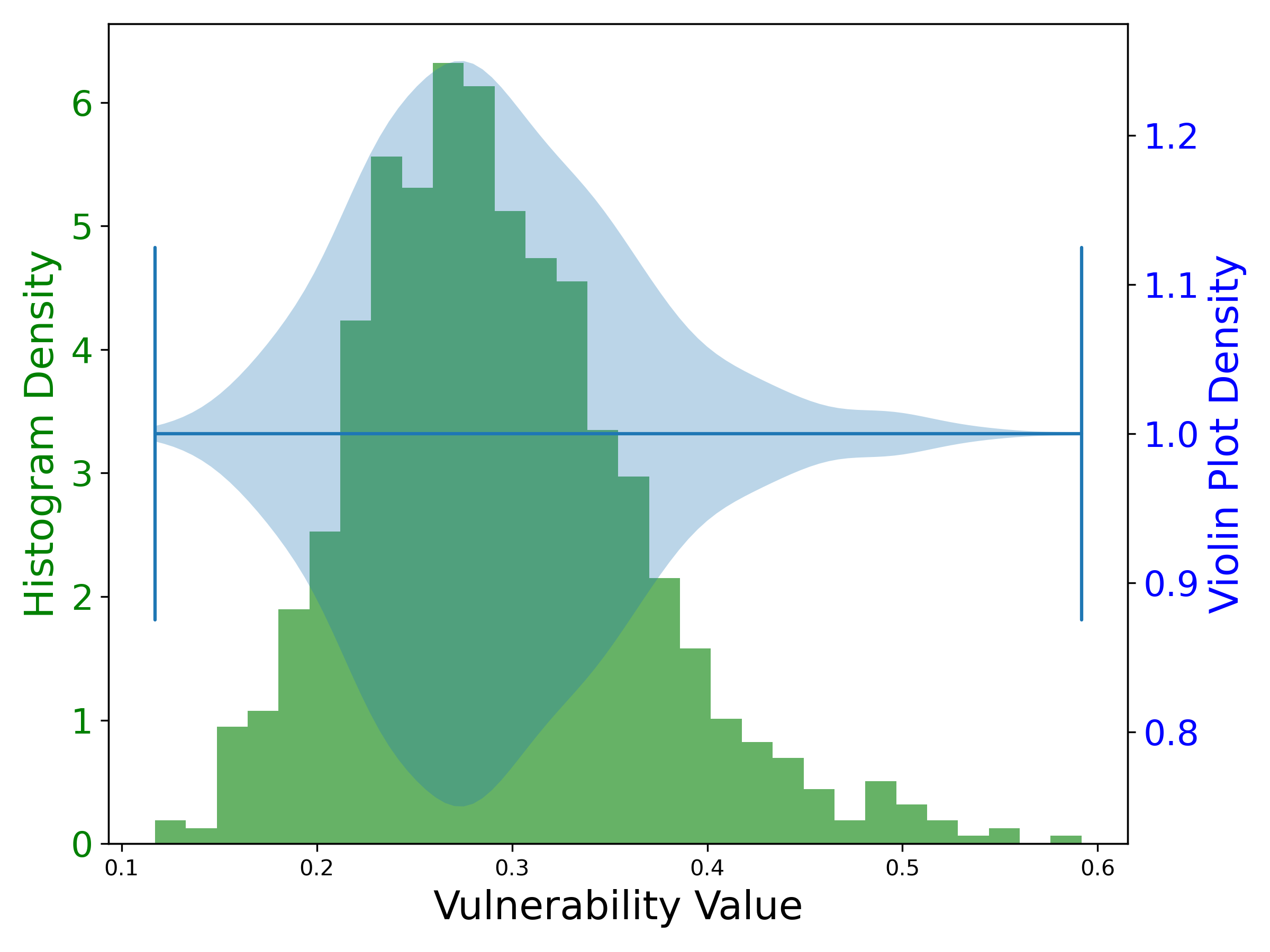
(a) 33-bus data

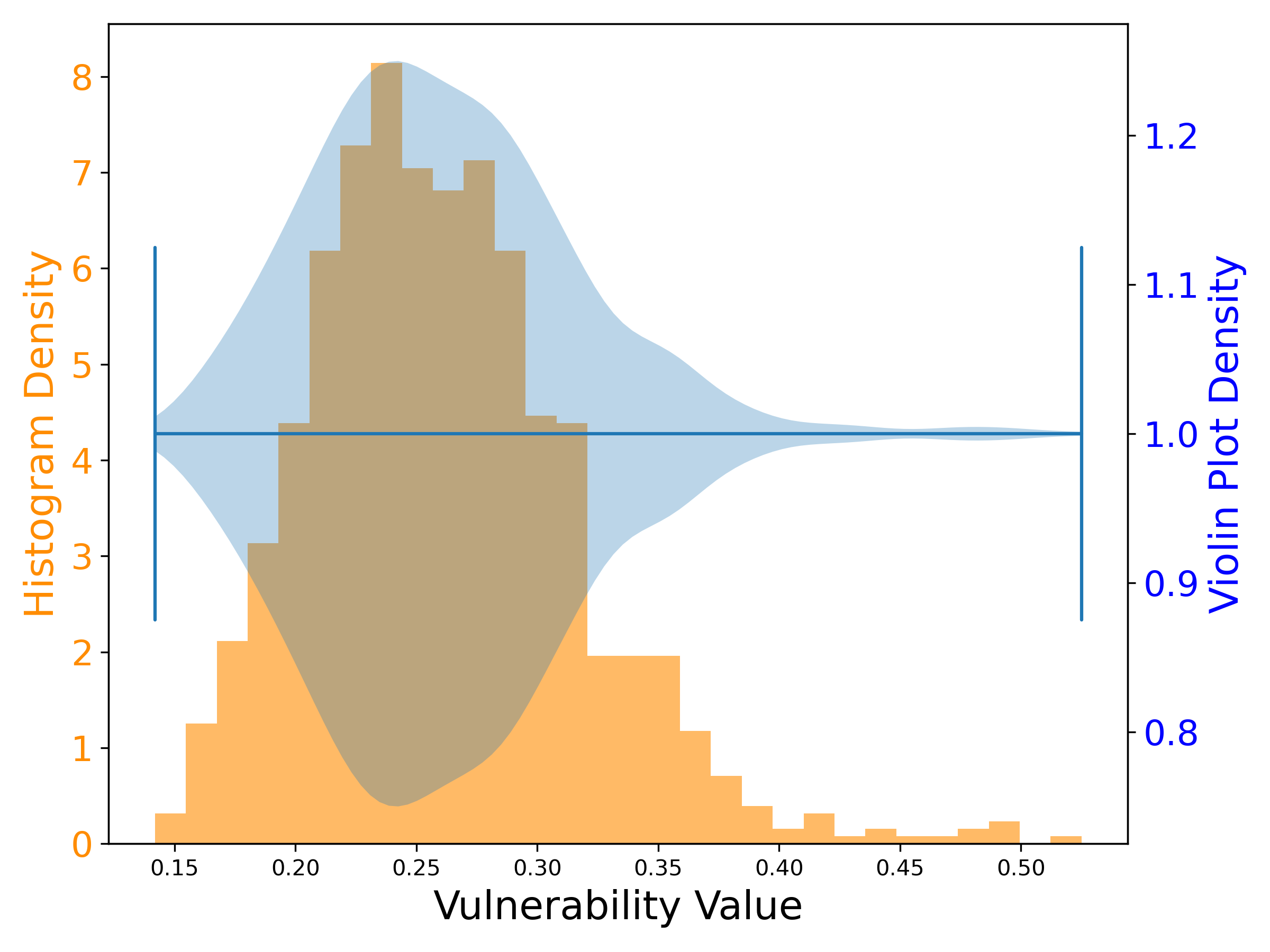
(b) 66-bus data

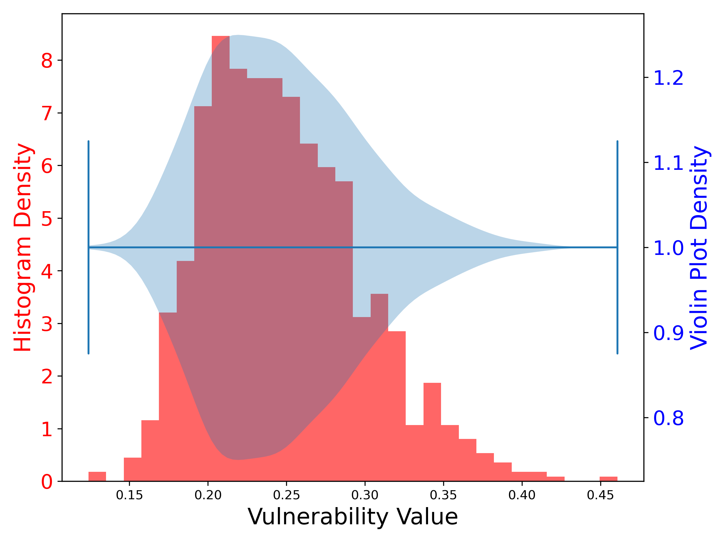
(c) 100-bus data

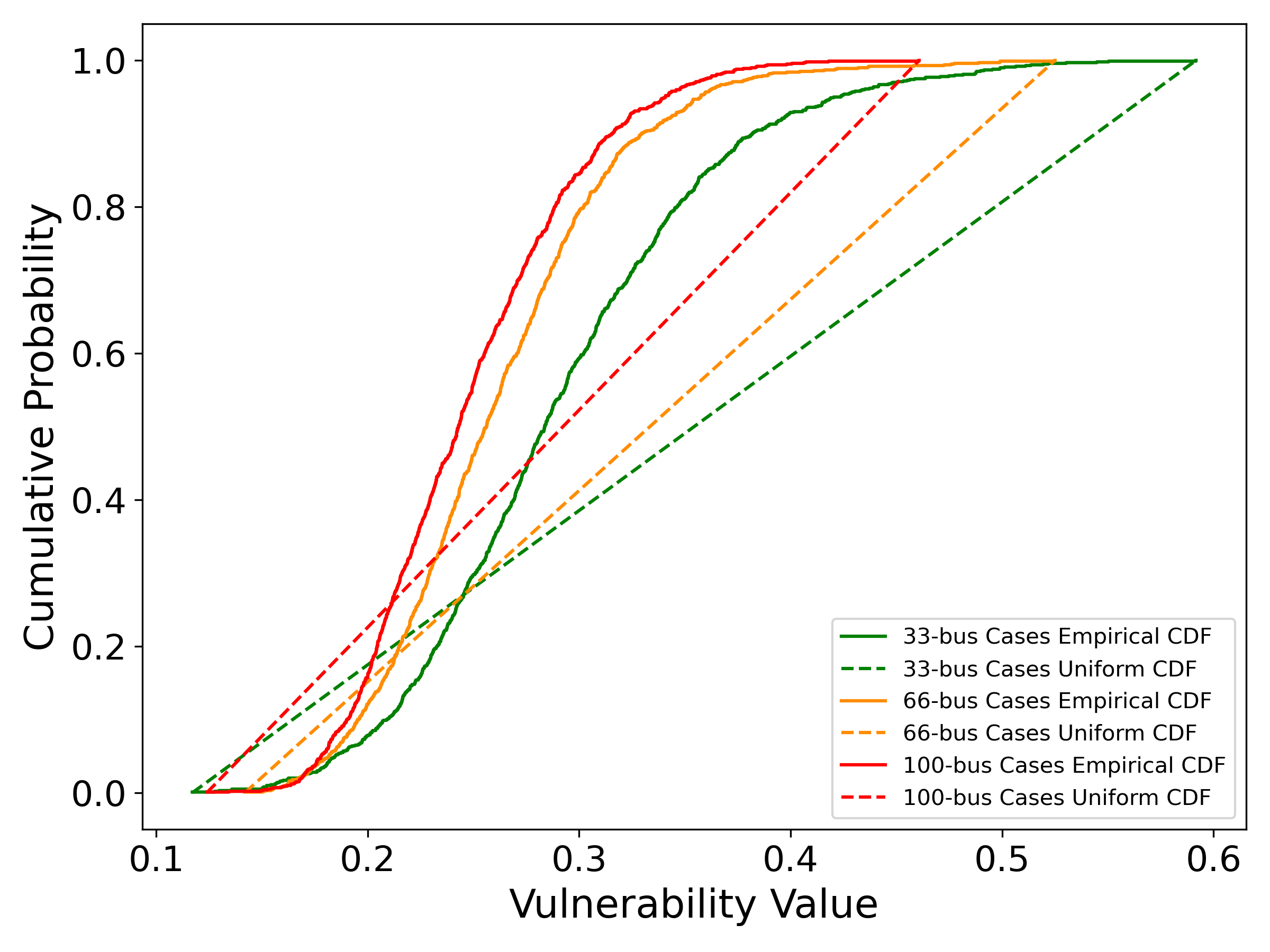
(d) CDF Curves

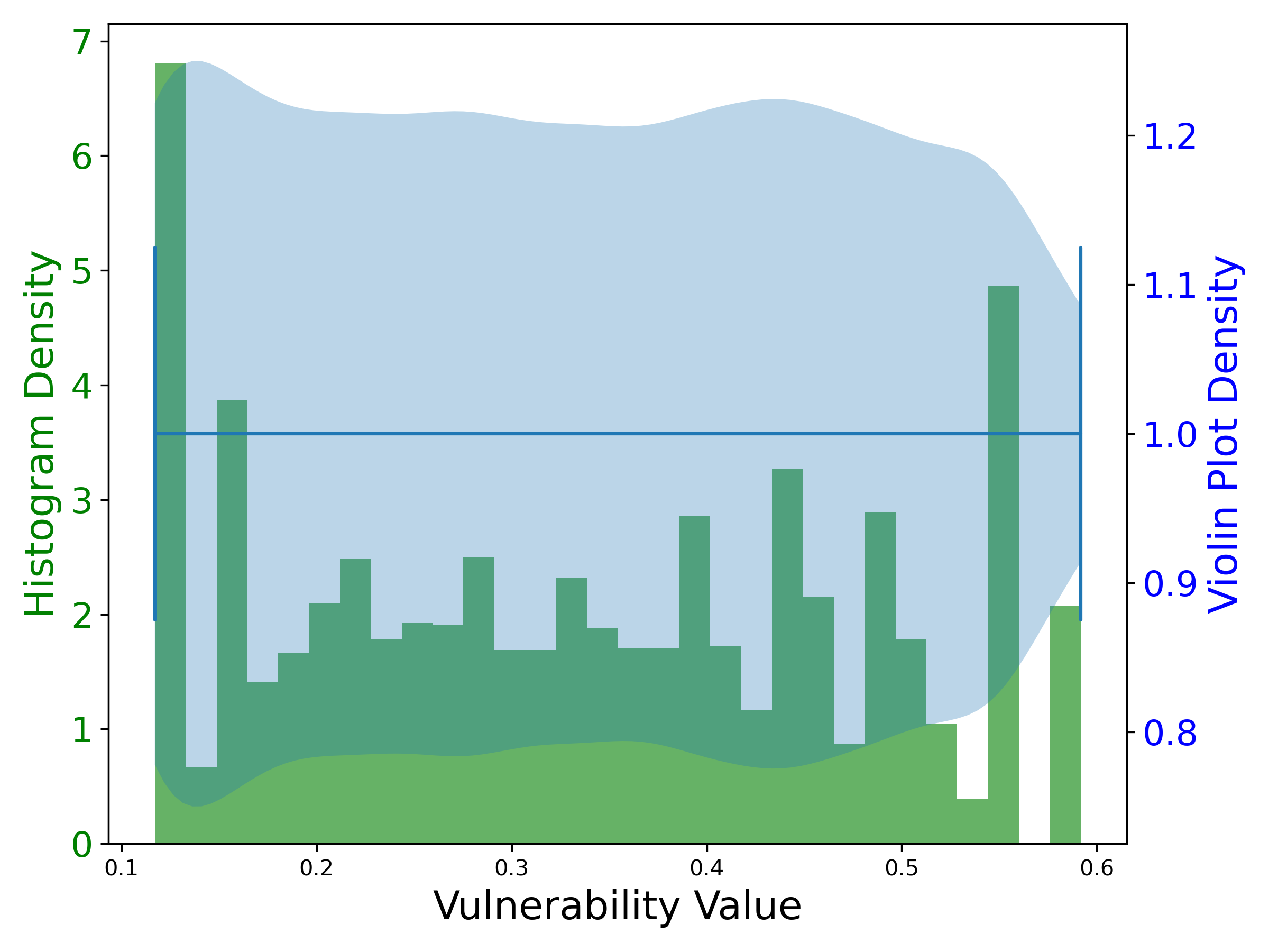
(e) Resampled 33-bus data

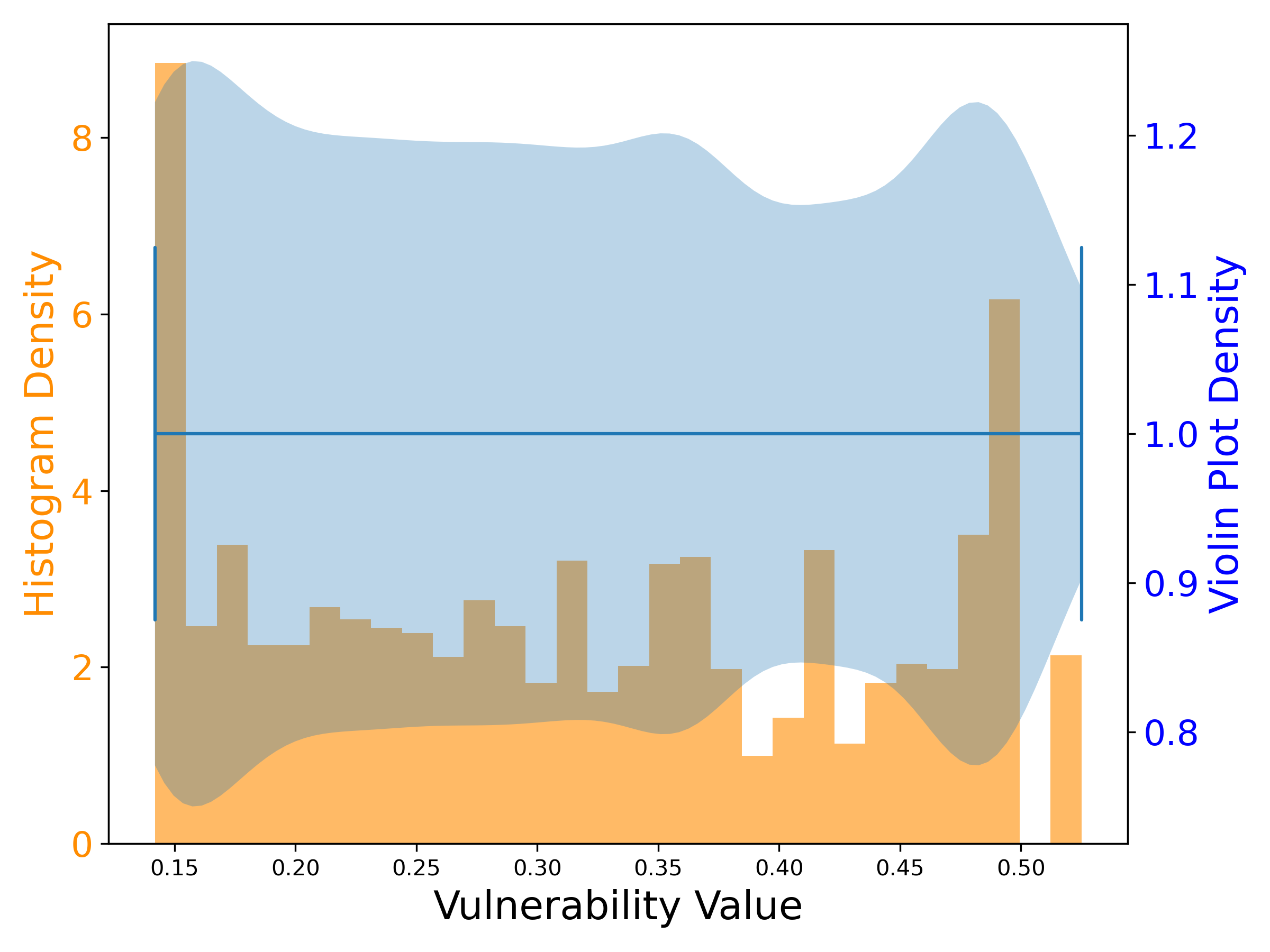
(f) Resampled 66-bus data

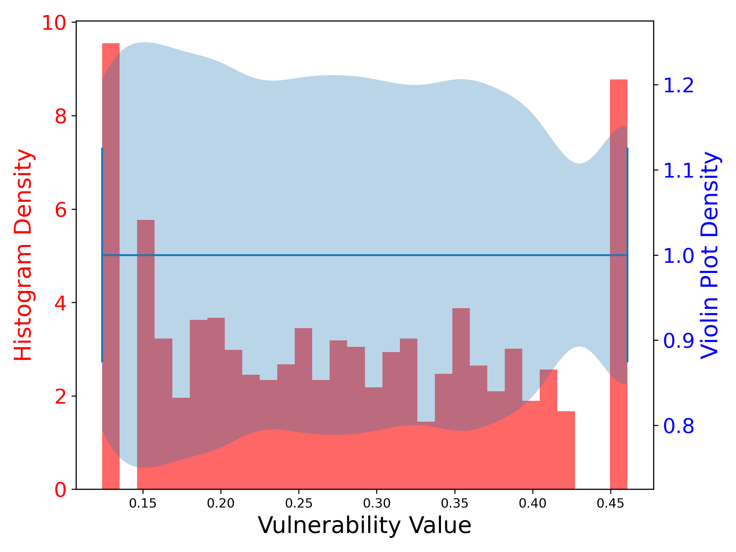
(g) Resampled 100-bus data

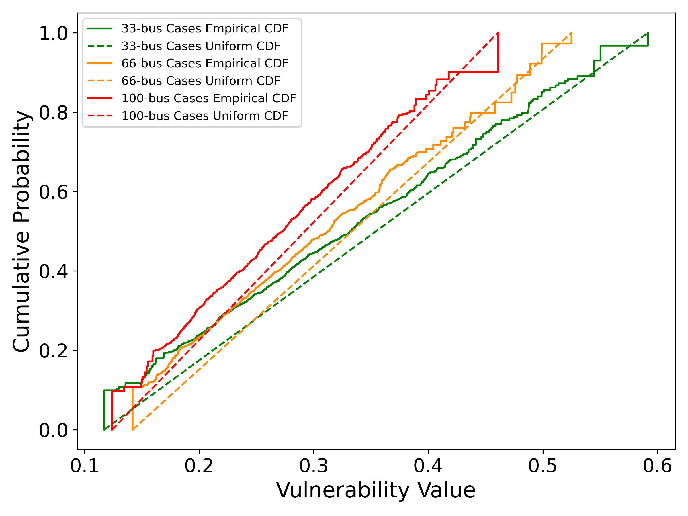
(h) CDF curves of the resampled data

Figure 3: The distributions of the generated training data and the resampled data respectively with the sizes of 33, 66, and 100. (d) and (h) respectively draw the CDF curves of the generated and resampled data distribution.

Three GAT-S models are respectively trained on the 33, 66, and 100-bus instances using 4000 samples over 100 epochs. The Adam optimizer is used here with a learning rate of 0.0001. Fig. 4 presents the loss curves, with red lines showing smoothed curves (smooth window of 200) and shaded areas reflecting volatility. All three training processes converge well. The training loss, calculated as the MSE between predictions and labels, takes 50 to 120 minutes for problem sizes 33, 66, and 100.

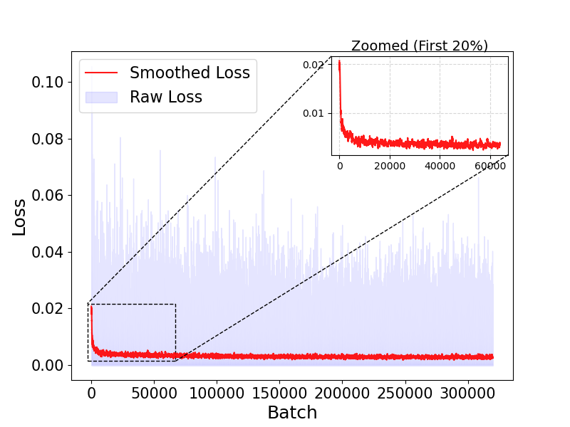
(a) Training process on 33-bus instances

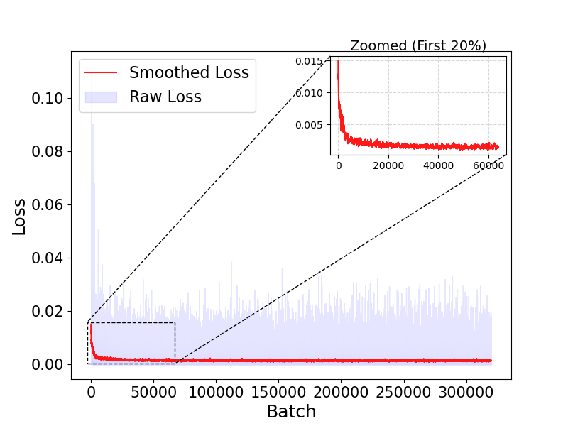
(b) Training process on 66-bus instances

(c) Training process on 100-bus instances

Figure 4: The model training process respectively on 33, 66, and 100-bus instances. The loss is defined as the MSE between the predicted values and the MCS-obtained baseline values.

IV-B Model Assessment

Fig. 5 illustrates a 33-bus test case: (a) microgrid topology (red points indicate generators, black points indicate loads), (b) active power data for loads and generators, (c) load shedding rate distribution from 500 simulated probabilistic attacks (scatter points show calculated rates per attack, shading indicates the data distribution curve), and (d) attention weights learned by the proposed GAT-S model (darker and higher bars on nodes indicate higher attention values).

GAT-S uses microgrid features as inputs to calculate vulnerability through a simple feed-forward process. Its self-attention pooling mechanism enhances explainability by using attention weights to highlight each bus’s contribution to grid-level vulnerability. As shown in Fig. 5(d), buses 11, 14, 17, 15, 30, 31, and 12 exhibit higher attention weights, corresponding to the presence of generators or higher node centrality. This indicates that nodes with generators and high centrality are more critical to microgrid vulnerability. These weights are shaped by the complex interaction of electrical and structural microgrid properties, beyond just node degree, making explainable machine-learning methods like GAT-S valuable for such analyses.

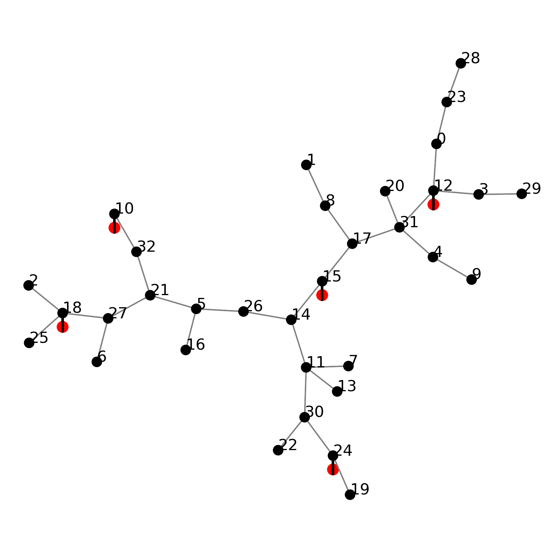
(a) Microgrid topology

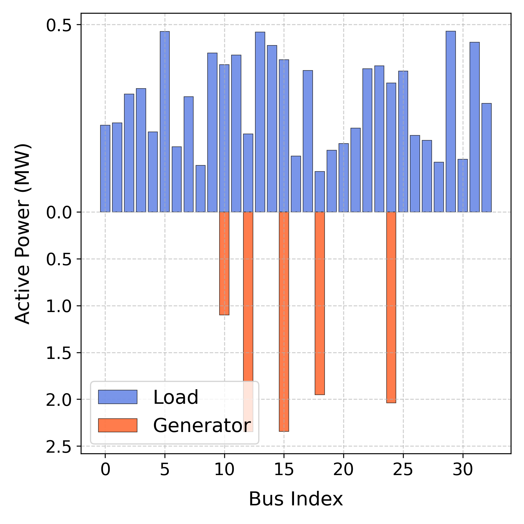
(b) Active power injection

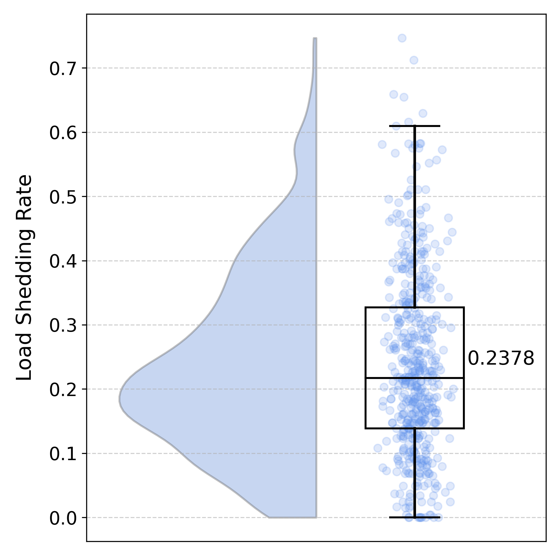
(c) MCS-obtained load shedding rates

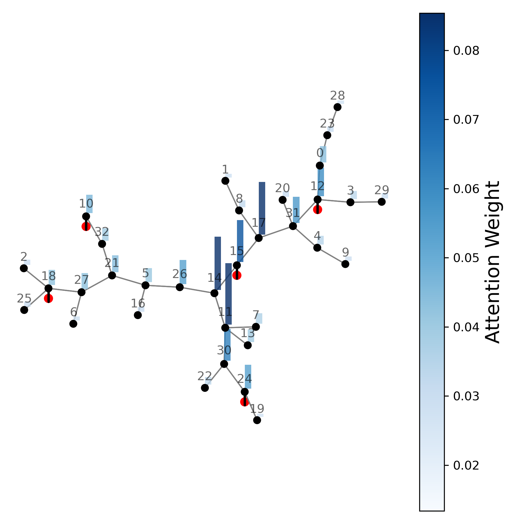
(d) GAT-S-obtained attention weights

Figure 5: The data distribution and assessment simulation through both MCS and GAT-S on a 33-bus test instance: (a) the microgrid topology, (b) active power injection data for the loads and generators, (c) the distribution of MCS-obtained load shedding rates from 500 simulated probabilistic attacks, and (d) self-learned attention weights obtained by the proposed GAT-S, indicating each bus’s contribution to the grid-level vulnerability.

IV-C Model Explainability

To delve deeper into the model explainability regarding node-level vulnerability, we first define the node-level vulnerability $V_{i}$ as the load shedding rate after a disruption on bus $i$ as below:

$$V_{i}=\frac{U_{i}}{L},$$ (17)

where $L$ is the total microgrid load demand, and $U_{i}$ is the unsatisfied load due to the disruption on bus $i$.

Using the same microgrid case as in Section IV-B, Fig. 6 visualizes the calculated node-level vulnerability values (red bars) and the learned attention weights (blue bars) for all buses. Darker and taller bars indicate higher values. The distributions of attention weights and node-level vulnerability values are generally similar across buses, highlighting the need to focus on buses 11, 14, 15, 17, 31, and 12. This offers a reliable foundation for future node hardening strategies. Additionally, while attention weights emphasize buses with generators, node-level vulnerability values are more evenly spread and target higher-degree buses. The differing distributions arise because attention weights prioritize node feature contributions for graph-level attention, while vulnerability values focus on node-level risks. Whereas, the attention weights offer an explainable framework, enhancing transparency and helping decision-makers identify critical nodes. This improvement is significant as its explainability stems from its learnable network parameters rather than relying on post-hoc tools like external feature selection algorithms [15], SHAP, or LIME methods [38]. Attention weights can be learned directly through the model’s feed-forward process, eliminating the need for additional calculations and analyses commonly found in current studies.

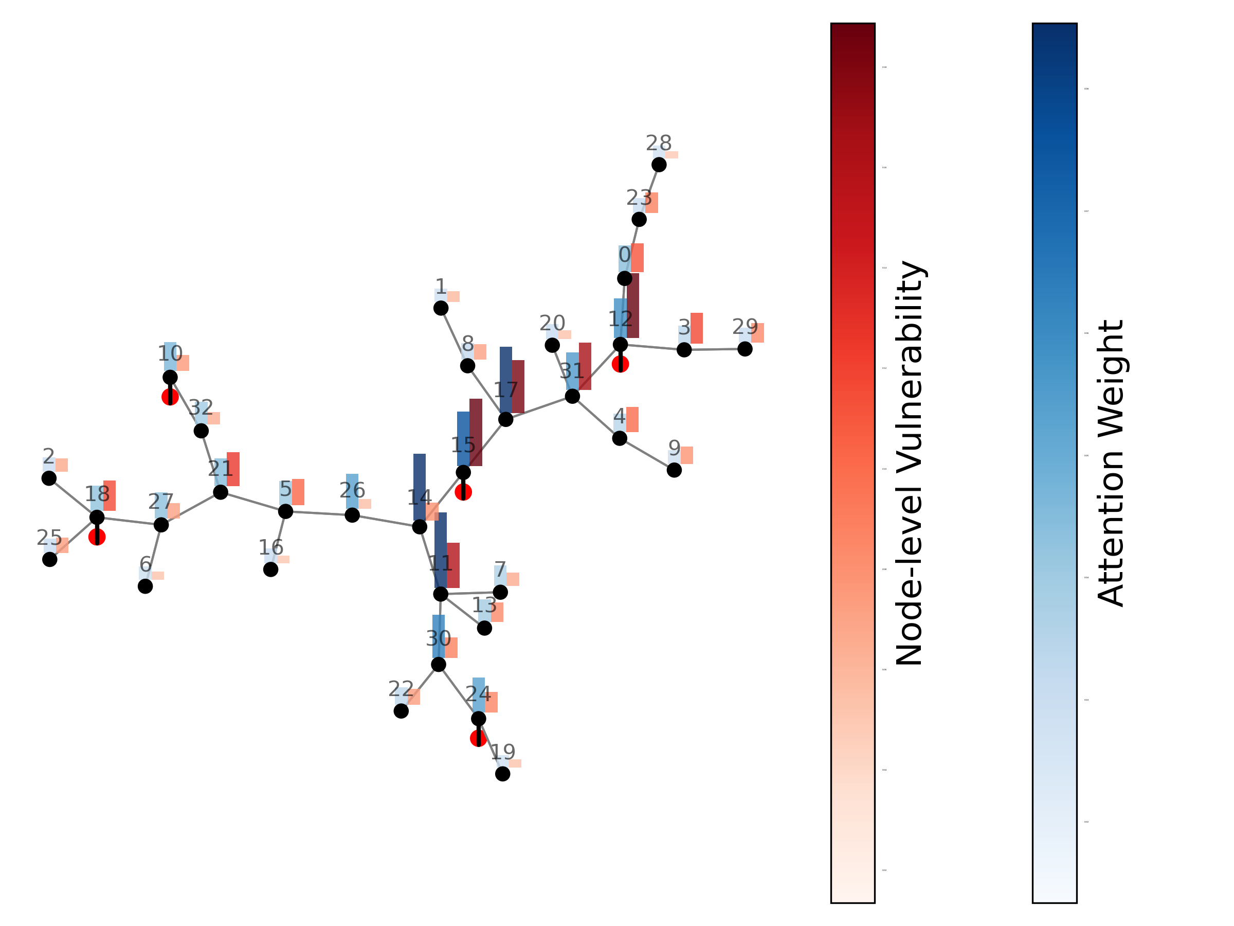
Figure 6: The calculated node-level vulnerability values (red bars) and the learned attention weights (blue bars) for all buses on a 33-bus independent microgrid test instance. Darker and taller bars on nodes indicate higher values.

IV-D Model Effectiveness

To evaluate the effectiveness of the proposed GAT-S, several ML-based methods, including Bayesian additive regression tree (BART) [12], deep neural network (DNN), and graph neural network (GNN) [15], are implemented for comparison. The DNN consists of a six-layer fully connected neural network with a hidden dimension of 64, employing the ReLU activation function. While the BART and GNN in the literature are not open-source, we reproduced them using their original parameter settings as closely as possible. To ensure fairness, all models are trained on the same dataset for 100 epochs. To optimize performance, BART, DNN, GNN, and GAT-S models are trained and tested on corresponding data sizes (e.g., models tested on 33-bus instances are trained on 33-bus instances). Additionally, MCS with 1000 iterations is used as the baseline. Model performance is measured through MSE, mean absolute error (MAE), and mean absolute percentage error (MAPE). The lower these metrics values, the more accurate the model prediction.

Table II presents the detailed experimental results, with the best-performing values highlighted in gray. As can be seen, the proposed GAT-S consistently outperforms DNN, BART, and GNN across all instances and all evaluation metrics. Compared with the MCS-obtained baseline values, GAT-S achieves an MSE as low as 0.001, while BART, DNN, and GNN generally have errors two to three times higher. In terms of runtime, DNN, GNN, and GAT-S demonstrate obvious superiority, generating results in one second. This efficiency is due to their reliance on a simple feed-forward calculation to produce predictions. Such rapid assessment is crucial for handling numerous objective evaluations in microgrid design optimization.

TABLE II: The comparison results of algorithms are presented for metrics such as MSE, MAE, MAPE, and runtimes, with the best values highlighted in gray. MCS serves as the baseline, while BART, DNN, GNN, and the proposed GAT-S are compared. 33, 66, and 100-bus microgrids respectively with the number of 100 serve as the test instances.

	33-Bus Instances				66-Bus Instances				100-Bus Instances
Methods	MSE	MAE	MAPE	Time(s)	MSE	MAE	MAPE	Time(s)	MSE	MAE	MAPE	Time(s)
MCS	/	/	/	115	/	/	/	212	/	/	/	294
BART	6.40E-03	6.35E-02	9.90E-02	37	2.90E-03	4.19E-02	5.95E-02	69	2.30E-03	3.90E-02	5.24E-02	106
DNN	7.80E-03	7.02E-02	1.09E-01	1	3.90E-03	4.92E-02	6.88E-02	1	3.20E-03	4.24E-02	5.82E-02	1
GNN	6.29E-03	5.74E-02	9.76E-02	1	3.42E-03	4.14E-02	6.53E-02	1	2.17E-03	3.47E-02	4.84E-02	1
GAT-S	4.16E-03	5.23E-02	7.90E-02	1	1.47E-03	2.88E-02	3.99E-02	1	1.02E-03	2.54E-02	3.46E-02	1

Fig. 7 visualizes the predicted values and MCS-derived baseline values for the 33, 66, and 100-bus test cases in the form of scatters. The horizontal axis represents predicted values, while the vertical axis shows the MCS baseline values. Different colors indicate different methods. Solid lines represent fitted trends for the scatter points, while dashed lines indicate the reference line $y=x$. The closer a fitted line is to $y=x$, the higher the prediction accuracy of the method. The proposed GAT-S demonstrates its advantages. In contrast, while BART and GNN perform not badly on metrics like MSE, their predictions tend to be conservative and show minimal variation around the mean. This means that they are essentially not valid on this assessment issue.

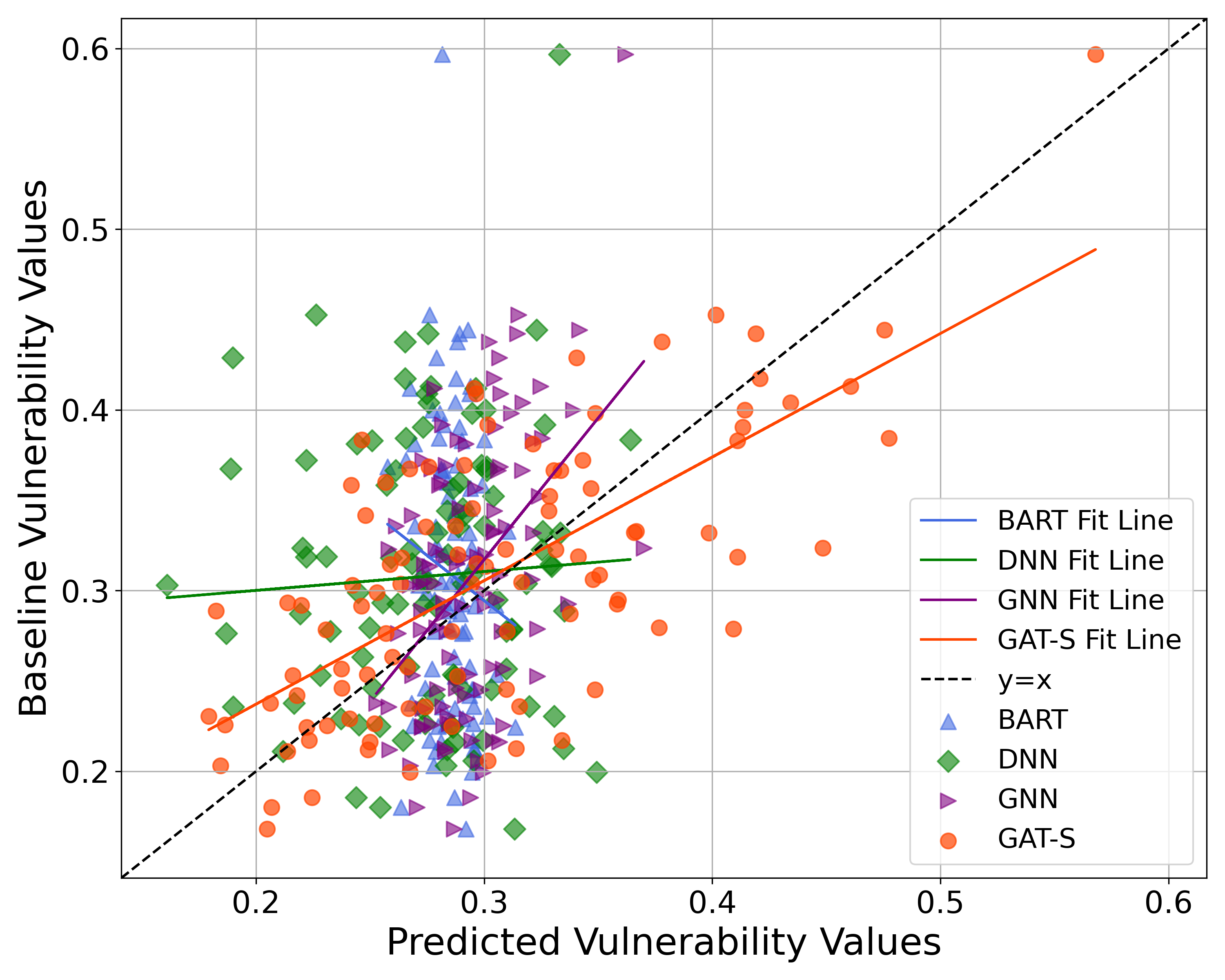
(a) Results on the 33-bus instances

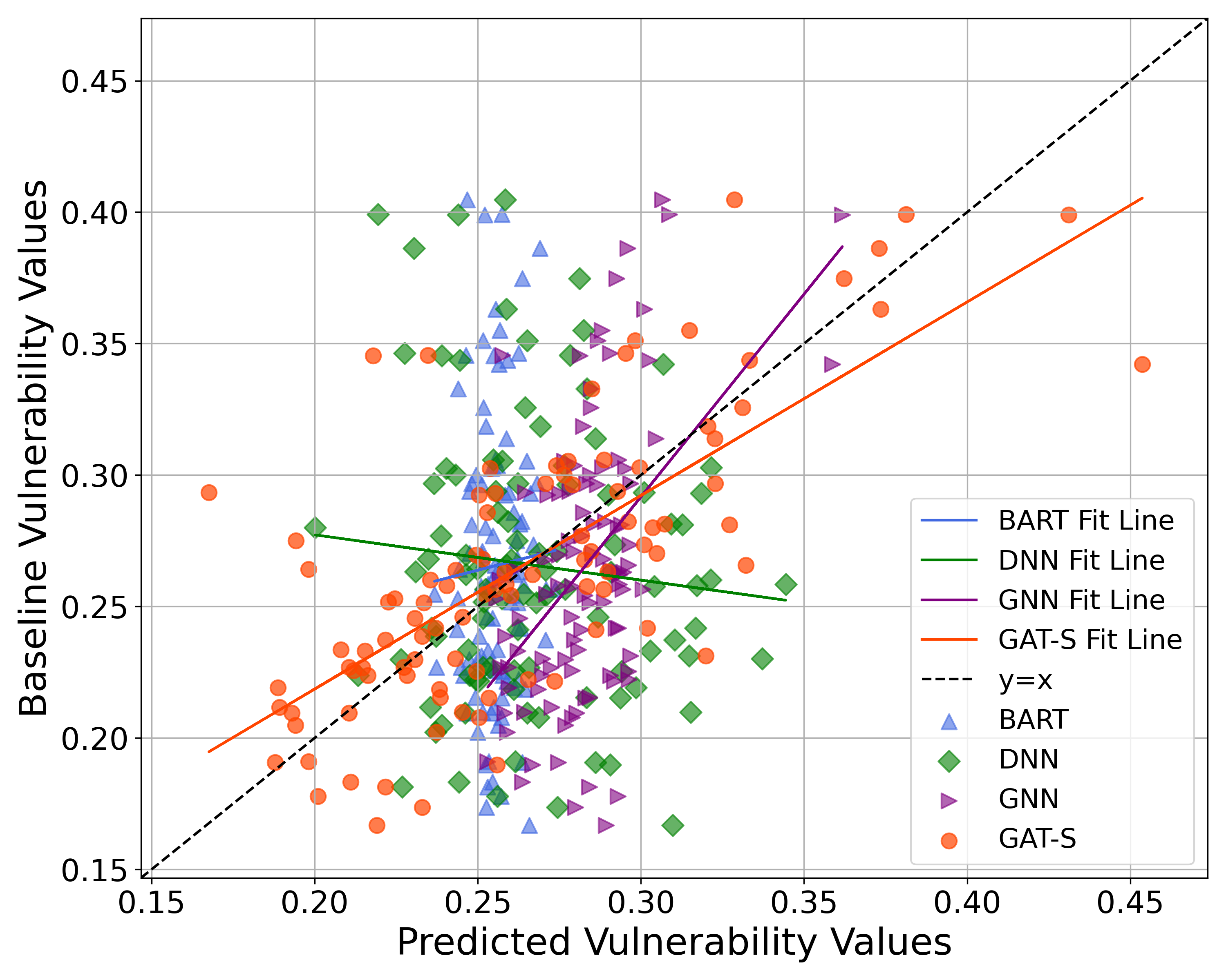
(b) Results on the 66-bus instances

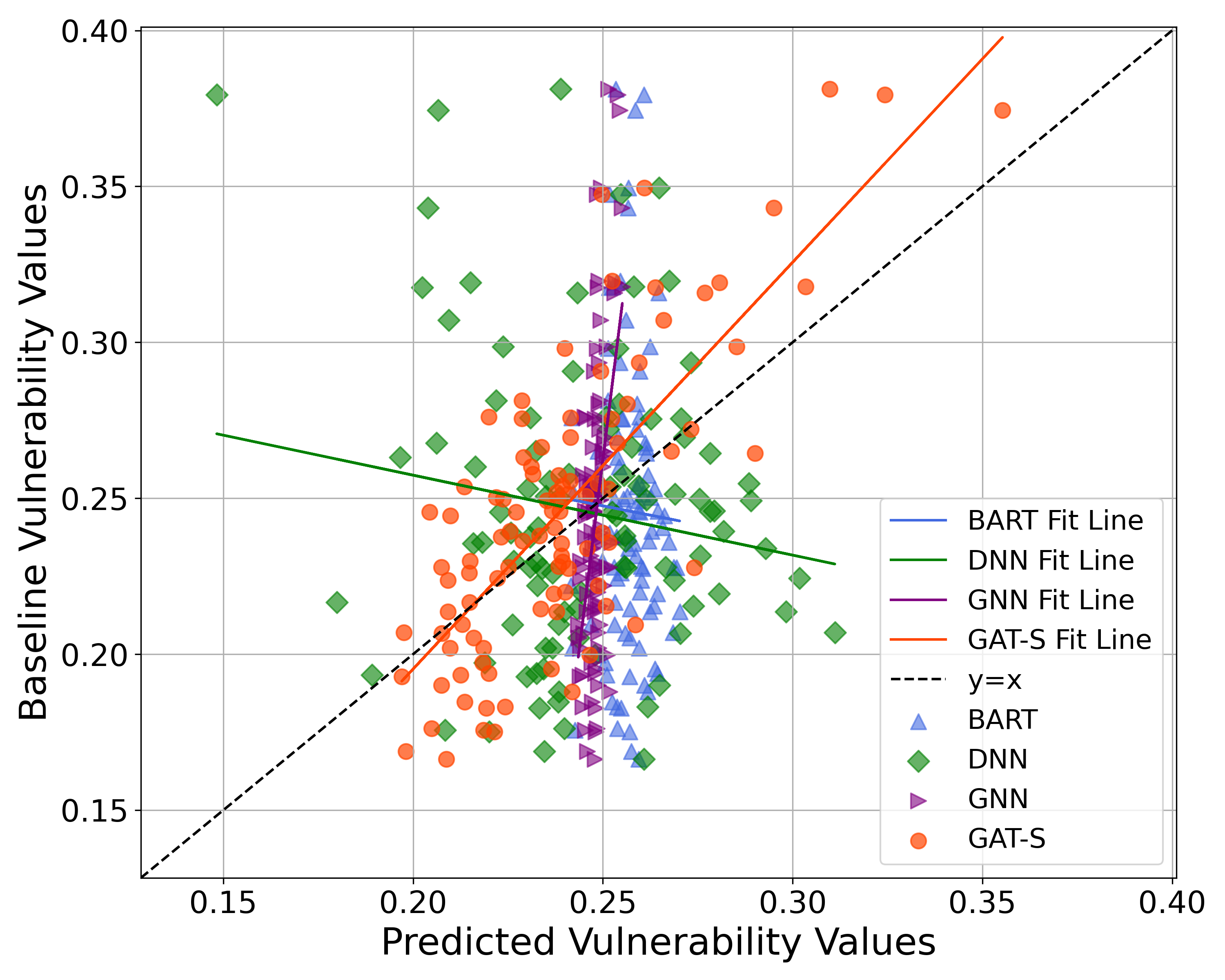
(c) Results on the 100-bus instances

Figure 7: Scatter plots compare predicted values from GAT-S, BART, DNN, and GNN with baseline values from MCS for the 33, 66, and 100-bus test cases. Fitted lines are included, with the black dashed line representing $y=x$.

IV-E Model Generalization Ability

IV-E1 Generalization on Problem Scales

To validate the generalization ability of the proposed GAT-S model on cases with different sizes, this subsection compares the performance of the GAT-S models respectively trained on the 33, 66, and 100-bus training instances (i.e., GAT-S-33, GAT-S-66, and GAT-S-100) on the test instances with the sizes of 33, 66, and 100. Meanwhile, a GAT-S model trained on all training instances (i.e., 33, 66, and 100-bus instances) is also in comparison and is named GAT-S-ALL. Table III lists the comparison results, with the metrics of MSE, MAE, and MAPE, and the best-performed values are highlighted in gray. According to the results, the model performs best when the training and test sizes match, with minor decreases in accuracy observed for differing problem sizes. This indicates that the evaluation accuracy of the pre-trained model remains reliable despite some variation in problem size. On the other hand, the GAT-S-ALL model, trained on 33, 66, and 100-bus instances, demonstrates medium performance on the 33 and 66-bus tests but excels on the 100-bus tests. While diverse training instances slightly reduce the model’s specificity to individual cases, they enhance its ability to generalize across different scales.

TABLE III: The comparison results of algorithms are presented for metrics such as MSE, MAE, and MAPE, with the best values highlighted in gray. MCS serves as the baseline, while GAT-S-33, GAT-S-66, GAT-S-100, and GAT-S-ALL are compared. 33, 66, and 100-bus microgrids respectively with the number of 100 serve as the test instances.

	33-Bus Instances			66-Bus Instances			100-Bus Instances
Methods	MSE	MAE	MAPE	MSE	MAE	MAPE	MSE	MAE	MAPE
GAT-S-33	4.16E-03	5.23E-02	7.90E-02	2.55E-03	4.08E-02	5.55E-02	1.77E-03	3.53E-02	4.66E-02
GAT-S-66	5.03E-03	5.62E-02	8.48E-02	1.47E-03	2.88E-02	3.99E-02	1.14E-03	2.75E-02	3.63E-02
GAT-S-100	6.77E-03	6.57E-02	1.01E-01	2.50E-03	4.14E-02	5.73E-02	1.02E-03	2.54E-02	3.46E-02
GAT-S-ALL	6.11E-03	6.48E-02	1.01E-01	1.70E-03	3.10E-02	4.42E-02	9.50E-04	2.44E-02	3.27E-02

IV-E2 Generalization on Generator Distributions

This subsection discusses the model’s generalization ability when the generator distribution changes. The GAT-S-33 model was trained on microgrids with 15% generators (i.e., 5 in total), while the experimental test instances consist of 33-bus microgrids with generator percentages from 10% to 80%, respectively including 20 cases for each percentage. All other parameters remained consistent with the prior test instances. Detailed experimental results, including MSE, MAE, and MAPE metrics, are presented in Table IV.

TABLE IV: Assessment results on 33-bus instances with different generator percentages. The pre-trained GAT-S-33 model is tested. MSE, MAE, and MAPE serve as metrics.

Generator Percentage	Metrics
	MSE	MAE	MAPE
10%	6.21E-03	6.42E-02	1.02E-01
20%	3.36E-03	4.94E-02	6.90E-02
30%	9.63E-03	8.51E-02	1.11E-01
40%	4.48E-02	1.98E-01	2.35E-01
50%	6.89E-02	2.59E-01	3.08E-01
60%	1.05E-01	3.21E-01	3.69E-01
70%	1.39E-01	3.71E-01	4.13E-01
80%	1.38E-01	3.69E-01	4.13E-01

Greater changes in the generator percentage lead to higher assessment errors. The pre-trained model experiences an MSE exceeding 0.01 when the percentage rises above 30%. This result indicates when to appropriately use this model, as its generalization ability is limited. While significant changes in the problem distribution can degrade the performance of pre-trained models, this is a common challenge faced by machine learning methods. Nevertheless, given the motivation of this study, that is, developing a fast and explainable surrogate model for microgrid optimization in planning, it essentially requires less emphasis on model generalization across varying problem sizes and generator percentages. In contrast, microgrid planning primarily focuses on optimizing equipment (e.g., distributed generators, energy storage, and movable loads) layout and connectivity, which are randomly generated in our test instances. The proposed GAT-S model has been validated as effective for these scenarios.

V Conclusion

This study proposes a fast and local explainable vulnerability assessment framework for independent microgrids by integrating Monte Carlo simulation with a graph attention network enhanced by self-attention pooling. The framework addresses key challenges in microgrid vulnerability assessment, including computational inefficiency, limited accuracy, and lack of explainability in existing methods. By leveraging MCS to generate training data and representing microgrids as graph-structured data, the GAT-S model effectively captures both structural and electrical characteristics, dynamically assigning attention weights to critical nodes. This approach enables accurate, explainable, and real-time vulnerability assessments, achieving an MSE as low as 0.001 in experiments on test instances with sizes of 33, 66, and 100. The model generalization ability on different problem sizes and generator distributions has also been validated.

The results demonstrate the framework’s ability to support iterative decision-making processes in microgrid design and risk prevention, offering significant improvements in both computational efficiency and model transparency. However, the current framework assumes static microgrid configurations and does not explicitly account for uncertainties in renewable energy generation or dynamic operational conditions. Future work will aim to enhance the ML-based framework by integrating these factors and assessing its scalability to larger, more complex power systems. Additionally, investigating the use of advanced artificial intelligence methods to improve model generalization is also a valuable research direction.

References

- [1] Z. Liu, P. Tang, K. Hou, L. Zhu, J. Zhao, H. Jia, and W. Pei, “A lagrange-multiplier-based reliability assessment for power systems considering topology and injection uncertainties,” IEEE transactions on power systems, vol. 39, no. 1, pp. 1178–1189, 2023.
- [2] P. Gasser, P. Lustenberger, M. Cinelli, W. Kim, M. Spada, P. Burgherr, S. Hirschberg, B. Stojadinovic, and T. Y. Sun, “A review on resilience assessment of energy systems,” Sustainable and Resilient Infrastructure, vol. 6, no. 5, pp. 273–299, 2021.
- [3] U. Shahzad, “Vulnerability assessment in power systems: a review,” Journal of Electrical Engineering, Electronics, Control and Computer Science, vol. 7, no. 4, pp. 17–24, 2021.
- [4] A. Abedi, L. Gaudard, and F. Romerio, “Power flow-based approaches to assess vulnerability, reliability, and contingency of the power systems: The benefits and limitations,” Reliability Engineering & System Safety, vol. 201, p. 106961, 2020.
- [5] M. M. Breve, B. Bohnet, G. Michalke, J. Kowal, and K. Strunz, “Flow-network-based method for the reliability analysis of decentralized power system topologies with a sequential monte-carlo simulation,” IEEE Transactions on Reliability, vol. 73, no. 2, pp. 1005–1019, 2024.
- [6] T. P. Abud, A. A. Augusto, M. Z. Fortes, R. S. Maciel, and B. S. Borba, “State of the art monte carlo method applied to power system analysis with distributed generation,” Energies, vol. 16, no. 1, p. 394, 2022.
- [7] J. Faraji, M. Aslani, H. Hashemi-Dezaki, A. Ketabi, Z. De Grève, and F. Vallée, “Reliability analysis of cyber–physical energy hubs: A monte carlo approach,” IEEE Transactions on Smart Grid, vol. 15, no. 1, pp. 848–862, 2023.
- [8] P. Jiang, Q. Zhou, and X. Shao, Surrogate-Model-Based Design and Optimization. Singapore: Springer, 2020. [Online]. Available: https://doi.org/10.1007/978-981-15-0731-1_7
- [9] C. Ling, W. Kuo, and M. Xie, “An overview of adaptive-surrogate-model-assisted methods for reliability-based design optimization,” IEEE Transactions on Reliability, vol. 72, no. 3, pp. 1243–1264, 2022.
- [10] G. Li, Y. Huang, Z. Bie, and T. Ding, “Machine-learning-based reliability evaluation framework for power distribution networks,” IET Generation, Transmission & Distribution, vol. 14, no. 12, pp. 2282–2291, 2020.
- [11] R. E. Stern, J. Song, and D. B. Work, “Accelerated monte carlo system reliability analysis through machine-learning-based surrogate models of network connectivity,” Reliability Engineering & System Safety, vol. 164, pp. 1–9, 2017.
- [12] N. L. Dehghani, S. Zamanian, and A. Shafieezadeh, “Adaptive network reliability analysis: Methodology and applications to power grid,” Reliability Engineering & System Safety, vol. 216, p. 107973, 2021.
- [13] T. Lin and C. Shang, “Reliability evaluation on a joint machine learning and optimization framework,” IEEE Transactions on Power Systems, vol. 36, no. 1, pp. 49–57, 2020.
- [14] Q. Zhou, J. Davidson, and A. Fouad, “Application of artificial neural networks in power system security and vulnerability assessment,” IEEE Transactions on Power Systems, vol. 9, no. 1, pp. 525–532, 1994.
- [15] B. Cao, X. Wu, and X. Wang, “Reliability evaluation of park-level electricity-hydrogen systems using explainable graph neural network,” IEEE Transactions on Smart Grid, vol. 15, no. 3, pp. 3316–3328, 2024.
- [16] Q. X. Lieu, K. T. Nguyen, K. D. Dang, S. Lee, J. Kang, and J. Lee, “An adaptive surrogate model to structural reliability analysis using deep neural network,” Expert Systems with Applications, vol. 189, p. 116104, 2022.
- [17] Z. Min, W. Muqing, Q. Lilin, A. Quanbiao, and L. Sixu, “Evaluation of cross-layer network vulnerability of power communication network based on multi-dimensional and multi-layer node importance analysis,” IEEE Access, vol. 10, pp. 67 181–67 197, 2021.
- [18] W. Zixin, M. Shihong, G. Shuyu, H. Ji, Y. Haoran, and M. Wandeng, “Node vulnerability evaluation of distribution network considering randomness characteristic of distributed generation output,” Electric Power Automation Equipment, vol. 41, no. 8, pp. 33–40, 2021.
- [19] J. Fang, C. Su, Z. Chen, H. Sun, and P. Lund, “Power system structural vulnerability assessment based on an improved maximum flow approach,” IEEE Transactions on Smart Grid, vol. 9, no. 2, pp. 777–785, 2016.
- [20] Z. Zhang, S. Huang, S. Mei, X. Zhang, and Y. Jiang, “Vunerability assessment method of branch lines in power grid based on cooperative game,” Automation Electr. Power Syst, vol. 44, no. 06, pp. 9–16, 2020.
- [21] P. Gautam, P. Piya, and R. Karki, “Resilience assessment of distribution systems integrated with distributed energy resources,” IEEE Transactions on Sustainable Energy, vol. 12, no. 1, pp. 338–348, 2020.
- [22] C. J. Kim and O. B. Obah, “Vulnerability assessment of power grid using graph topological indices,” International Journal of Emerging Electric Power Systems, vol. 8, no. 6, 2007.
- [23] Z. Shen, C. Gu, Q. Wu, and J. Qian, “Early warning of fault in active distribution networks based on dynamic power flow motifs,” in 2022 2nd International Conference on Consumer Electronics and Computer Engineering (ICCECE), 2022, pp. 108–112.
- [24] X. Wang, C. Hao, X. Li, S. Sun, and W. Shi, “The vulnerability analysis of distribution network with distributed gene-ration,” Electr. Meas. Instrum, vol. 16, no. 6, pp. 38–43, 2019.
- [25] T. Wang, X. Yue, X. Gu et al., “Comprehensive evaluation of power grid vulnerability based on hesitant fuzzy decision making method,” Power Syst. Technol., vol. 41, no. 7, pp. 2272–2281, 2017.
- [26] A. Escalera, B. Hayes, and M. Prodanović, “A survey of reliability assessment techniques for modern distribution networks,” Renewable and Sustainable Energy Reviews, vol. 91, pp. 344–357, 2018.
- [27] A. Tabares, G. Munoz-Delgado, J. F. Franco, J. M. Arroyo, and J. Contreras, “An enhanced algebraic approach for the analytical reliability assessment of distribution systems,” IEEE Transactions on Power Systems, vol. 34, no. 4, pp. 2870–2879, 2019.
- [28] K. Zou, A. P. Agalgaonkar, K. M. Muttaqi, and S. Perera, “An analytical approach for reliability evaluation of distribution systems containing dispatchable and nondispatchable renewable dg units,” IEEE Transactions on smart grid, vol. 5, no. 6, pp. 2657–2665, 2014.
- [29] G. Muñoz-Delgado, J. Contreras, and J. M. Arroyo, “Reliability assessment for distribution optimization models: A non-simulation-based linear programming approach,” IEEE Transactions on Smart Grid, vol. 9, no. 4, pp. 3048–3059, 2016.
- [30] C. Wang, T. Zhang, F. Luo, P. Li, and L. Yao, “Fault incidence matrix based reliability evaluation method for complex distribution system,” IEEE Transactions on Power Systems, vol. 33, no. 6, pp. 6736–6745, 2018.
- [31] R. He, H. Liang, J. Wu, H. Xie, and M. Shahidehpour, “Reliability assessment of cyber-physical distribution system using multi-dimensional information network model,” IEEE Transactions on Smart Grid, vol. 14, no. 6, pp. 4683–4692, 2023.
- [32] A. M. L. Da Silva and A. M. De Castro, “Risk assessment in probabilistic load flow via monte carlo simulation and cross-entropy method,” IEEE Transactions on Power Systems, vol. 34, no. 2, pp. 1193–1202, 2018.
- [33] N. Nikmehr and P. Zhang, “Quantum-inspired power system reliability assessment,” IEEE Transactions on Power Systems, vol. 38, no. 4, pp. 3476–3490, 2022.
- [34] K. Zhou, I. Dobson, and Z. Wang, “The most frequent nk line outages occur in motifs that can improve contingency selection,” IEEE Transactions on Power Systems, vol. 39, no. 1, pp. 1785–1796, 2023.
- [35] G. Chen, Z. Y. Dong, D. J. Hill, G. H. Zhang, and K. Q. Hua, “Attack structural vulnerability of power grids: A hybrid approach based on complex networks,” Physica A: Statistical Mechanics and its Applications, vol. 389, no. 3, pp. 595–603, 2010.
- [36] M. B. Cain, R. P. O’neill, A. Castillo et al., “History of optimal power flow and formulations,” Federal Energy Regulatory Commission, vol. 1, pp. 1–36, 2012.
- [37] A. Kargarian, J. Mohammadi, J. Guo, S. Chakrabarti, M. Barati, G. Hug, S. Kar, and R. Baldick, “Toward distributed/decentralized dc optimal power flow implementation in future electric power systems,” IEEE Transactions on Smart Grid, vol. 9, no. 4, pp. 2574–2594, 2016.
- [38] A. M. Salih, Z. Raisi-Estabragh, I. B. Galazzo, P. Radeva, S. E. Petersen, K. Lekadir, and G. Menegaz, “A perspective on explainable artificial intelligence methods: Shap and lime,” Advanced Intelligent Systems, p. 2400304, 2024.