Bayesian inference for dynamic spatial quantile models with interactive effects

Abstract

With the rapid advancement of information technology and data collection systems, large-scale spatial panel data presents new methodological and computational challenges. This paper introduces a dynamic spatial panel quantile model that incorporates unobserved heterogeneity. The proposed model captures the dynamic structure of panel data, high-dimensional cross-sectional dependence, and allows for heterogeneous regression coefficients. To estimate the model, we propose a novel Bayesian Markov Chain Monte Carlo (MCMC) algorithm. Contributions to Bayesian computation include the development of quantile randomization, a new Gibbs sampler for structural parameters, and stabilization of the tail behavior of the inverse Gaussian random generator. We establish Bayesian consistency for the proposed estimation method as both the time and cross-sectional dimensions of the panel approach infinity. Monte Carlo simulations demonstrate the effectiveness of the method. Finally, we illustrate the applicability of the approach through a case study on the quantile co-movement structure of the gasoline market.

Keywords: Dynamic panel, endogeneity, factor models, heterogenous spatial effects, high dimensional data.

JEL classification: C31, C33, E44

1 Introduction

Spatial panel data analysis concerns the spatial interactions of individuals and provides useful tools to a wide range of applications; Housing Economics Beenstock and Felsenstein (2015), Marketing Hunneman et al. (2022), Urban economics Glaser et al. (2022), to name a few. This paper introduces new spatial panel data model, namely, dynamic spatial panel quantile model with interactive effects, and investigates estimation and its theoretical property in the context of Bayesian framework. There is a large body of studies on “linear” panel models with interactive effects (e.g., Ando and Bai (2017), Bai (2009), Bai and Li (2012), Bai and Liao (2016), Bai and Ng (2002, 2013), Hallin and Li$\check{s}$ka (2007), Harding et al. (2020), Moon and Weidner (2015), Pesaran (2006), Stock and Watson (2002), Lu and Su (2016), among others), as well as “linear” spatial panel data models (Aquaro et al. (2021), Baltagi (2011), Bai and Li (2021), Kelejian and Prucha (2004), Lee (2004), Lin and Lee (2010), Li (2017), Lu (2017) Qu and Lee (2015), Reich et al. (2011), Shi and Lee (2017), Yu et al. (2008), among others). In contrast, however, studies that allow us to explore a quantile structure of large panel data models with interactive effects are scant.

Recently, Ando and Bai (2020) studied a panel quantile model with interactive effects and applied their method to the analysis of U.S. stock market data. Quantile regression (Koenker and Bassett (1978)) is a useful tool for estimating the effect of explanatory variables on the entire distribution of a response variable. Ando and Bai (2020)’s approach accommodates quantile co-movements under the heterogeneous slope coefficients. To further accommodate spatial interactions among the individual units, Ando et al. (2023) extended Ando and Bai (2020) by introducing a spatial panel quantile model with with interactive effects. Because these studies investigated static panel data, a natural direction is how to investigate the dynamic versions of these models. This paper develops a new Bayesian method for analyzing the dynamic spatial quantile panel model by jointly accommodating dynamic structure as well as spatial interactions among individual time series. Our approach allows the quantile analysis of the spatial and factor dependence under the assumption that the heterogeneous slope coefficients.

Because of the dynamic structure of data and large number of individuals, the number of parameters in the model is enormous. This poses several estimation challenges in the estimation when we develop a new Bayesian Markov chain Monte Carlo (MCMC) estimation procedure. First, because the quantile function is implicit to its coefficients, a Gibbs sampler does not exist. Other numeric methods such as importance sampling, Metropolis-Hastings algorithm and Hamiltonian Monte Carlo methods are impractical in front of the large dimensionality and the data generating process’s recursive nature. We randomise the quantile dynamics to create conditional conjugacy. Second, for standard Asymmetric Laplace representation in a Bayesian quantile regression model, using the auxiliary inverse Gaussian random variable Chhikara (1988) is likely to encounter the overflow problem when its kurtosis is high. We create a Chi square approximation to control for its tail behavior. Third, the spatial parameter is structural, therefore no existing Gibbs sampler is available in the literature. We borrow the idea from structural vector autoregression to propose a bimodal mixture distribution and implement it as a Gibbs sampler. Lastly, the ultra high dimension slows the computation of matrix operations. We apply the breadth-first-search algorithm from Graphical theory to blockalise the spatial matrix to reduce computational cost. Therefore, our novel MCMC algorithm expends not only the frontier of large-scale panel data but also Bayesian literature.

To support our method theoretically, we establish the Bayesian consistency. We note that such results for panel data models with interactive effects were never established before. To show such result, we will encounter several theoretical challenges, such as dynamic nature of model, large dimensional incidental parameters due to the loadings and factors, the nonsmooth objective function for the quantile regression, the nonlinearity arising from the spatial term, as well as the separation from regression coefficients and the loadings and factors because of the rotational indeterminacy of the latter. Some of these theoretical challenges have been studied by some recent studies, such as Ando and Bai (2020); Ando et al. (2023), Chen et al. (2021). Although these studies provide some useful tools to analyze the current model but we note that these results are established under a frequentist framework and we create a novel argument for our Bayesian frameowork.

Our contributions are summarized as follows. First, a dynamic spatial panel quantile model with interactive effects under heterogeneous slope coefficients is introduced. Second, a new Bayesian parameter estimation procedure is proposed. Third, Bayesian consistency is developed. Finally, we apply the proposed model and the estimation method to study the Australian gasoline market.

The paper is organized as follows. Section 2 introduces a new spatial panel quantile model with interactive fixed effects, and then presents a set of assumptions. In Section 3, we introduce new Bayesian MCMC estimation procedure. Section 4 provides Bayesian consistency of the proposed method. In Section 5, the proposed method is applied to Australian gasoline market. Section 6 provides our concluding remarks. To save space, all technical proofs are provided in the online supplementary document. The online supplementary document also contains Monte Carlo simulation results, which indicate that the proposed estimation procedure works well.

Notations Let $\|A\|$ = $[\mathrm{tr}(A^{\prime}A)]^{1/2}$ be the Frobenius norm of matrix $A$, where “tr” denotes the trace of a square matrix, and let $\|A\|_{2}$ be its spectrum norm (the largest singular value of $A$). In addition, for any $N\times N$ matrix $\|A\|_{1}$ is defined as $\|A\|_{1}=\max_{1\leq j\leq N}$ $\sum_{i=1}^{N}|a_{ij}|$ where $a_{ij}$ is the $(i,j)$-th element of $A$. Similarly, $\|A\|_{\infty}=\max_{1\leq i\leq N}\sum_{j=1}^{N}|a_{ij}|$. For sequences $a_{n}$ and $b_{n}$, the notation $a_{n}\lesssim b_{n}$ means $a_{n}=O(b_{n})$, that is, there exists $C>0$ and for all $n$ large enough, $a_{n}\leq Cb_{n}$. We write $c_{n}=O_{p}(d_{n})$ if $c_{n}/d_{n}$ is stochastically bounded, and $c_{n}=o_{p}(d_{n})$ if $c_{n}/d_{n}$ converges to zero in probability.

2 Dynamic spatial quantile models with interactive effects

2.1 Model

Suppose that, for the $i$-th unit $(i=1,...,N)$ at time $t$ $(t=1,...,T)$, its response $y_{it}$ is observed together with a set of $p$ explanatory variables $\{x_{it,1},...,x_{it,p}\}$. We consider the $\tau$-th quantile function of $y_{it}$ by jointly modeling spatial effects, time effects and common shocks. To capture these effects simultaneously, we define the $\tau$-th quantile function of $y_{it}$ as

$$Q_{y_{it}}\Big{(}\tau|X_{t},F_{t,\tau},B_{\tau},\Lambda_{\tau},\mbox{\boldmath$\rho$}_{\tau},\mbox{\boldmath$\gamma$}_{\tau},\mbox{\boldmath$\delta$}_{\tau}\Big{)}$$

$$\equiv\rho_{i,\tau}\sum_{i\neq j,j=1}^{N}w_{ij}Q_{y_{jt}}\Big{(}\tau|X_{t},F_{t,\tau},B_{\tau},\Lambda_{\tau},\mbox{\boldmath$\rho$}_{\tau},\mbox{\boldmath$\gamma$}_{\tau},\mbox{\boldmath$\delta$}_{\tau}\Big{)}$$

$$\quad+\delta_{i,\tau}\sum_{i\neq j,j=1}^{N}w_{ij}Q_{y_{j,t-1}}\Big{(}\tau|X_{t-1},F_{t-1,\tau},B_{\tau},\Lambda_{\tau},\mbox{\boldmath$\rho$}_{\tau},\mbox{\boldmath$\gamma$}_{\tau},\mbox{\boldmath$\delta$}_{\tau}\Big{)}$$

$$\quad+\gamma_{i,\tau}Q_{y_{i,t-1}}\Big{(}\tau|X_{t-1},F_{t-1,\tau},B_{\tau},\Lambda_{\tau},\mbox{\boldmath$\rho$}_{\tau},\mbox{\boldmath$\gamma$}_{\tau},\mbox{\boldmath$\delta$}_{\tau}\Big{)}+\sum_{k=1}^{p}x_{it,k}b_{ik,\tau}+\sum_{k=1}^{r}f_{tk,\tau}\lambda_{ik,\tau}+G_{i,e_{it}}^{-1}(\tau)$$

$$\equiv\rho_{i,\tau}\sum_{i\neq j,j=1}^{N}w_{ij}Q_{y_{jt}}\Big{(}\tau|X_{t},F_{t,\tau},B_{\tau},\Lambda_{\tau},\mbox{\boldmath$\rho$}_{\tau},\mbox{\boldmath$\gamma$}_{\tau},\mbox{\boldmath$\delta$}_{\tau}\Big{)}$$

$$\quad+\delta_{i,\tau}\sum_{i\neq j,j=1}^{N}w_{ij}Q_{y_{j,t-1}}\Big{(}\tau|X_{t-1},F_{t-1,\tau},B_{\tau},\Lambda_{\tau},\mbox{\boldmath$\rho$}_{\tau},\mbox{\boldmath$\gamma$}_{\tau},\mbox{\boldmath$\delta$}_{\tau}\Big{)}$$

$$\quad+\gamma_{i,\tau}Q_{y_{i,t-1}}\Big{(}\tau|X_{t-1},F_{t-1,\tau},B_{\tau},\Lambda_{\tau},\mbox{\boldmath$\rho$}_{\tau},\mbox{\boldmath$\gamma$}_{\tau},\mbox{\boldmath$\delta$}_{\tau}\Big{)}+\mbox{\boldmath$x$}_{it}^{\prime}\mbox{\boldmath$b$}_{i,\tau}+\mbox{\boldmath$f$}_{t,\tau}^{\prime}\mbox{\boldmath$\lambda$}_{i,\tau}$$ (1)

for $i=1,\dots,N$ and $t=1,\dots,T$. Here $w_{ij}$ $(i=1,2,\cdots,N;j=1,2,\cdots,N)$ are pre-specified spatial weights with $w_{ii}=0$, $\rho_{i,\tau}$ and $\delta_{i,\tau}$ are the heterogeneous spatial parameters capturing the strength of the spillover effects, the coefficients $\gamma_{i,\tau}$ are the heterogeneous temporal parameters, $\mbox{\boldmath$x$}_{it}=(1,x_{it,1},...,x_{it,p})^{\prime}$ is $(p+1)$ -dimensional vector of explanatory variables; $B_{\tau}=(\mbox{\boldmath$b$}_{1,\tau},\mbox{\boldmath$b$}_{2,\tau},\dots,\mbox{\boldmath$b$}_{N,\tau})^{\prime}$, $\mbox{\boldmath$b$}_{i,\tau}=(b_{i,0,\tau},b_{i,1,\tau},...,b_{i,p,\tau})^{\prime}$ is a $(p+1)$-dimensional vector of regression coefficients; $\mbox{\boldmath$f$}_{t,\tau}$ is $r_{\tau}$-dimensional unobservable common factors; $\mbox{\boldmath$\lambda$}_{\tau}$ is $r_{\tau}$-dimensional vector of factor loadings; $X_{t}$ and $F_{t,\tau}$ are information on the explanatory variables and the common factors up to time $t$; $e_{it}$ is the idiosyncratic error term and $G_{i,e_{it}}^{-1}(\tau)$ is the $\tau$-th quantile point of $e_{it}$ with $G_{i,e_{it}}(\cdot)$ being the cumulative distribution function of $e_{it}$. We assume that $e_{it}$ is identically distributed over $t$ while its distribution may vary over $i$. We note that the $\tau$-th quantile of the idiosyncratic error $G_{i,e_{it}}^{-1}(\tau)$, which depends only on $i$ and $\tau$, is absorbed by the term $\mbox{\boldmath$x$}_{it}^{\prime}\mbox{\boldmath$b$}_{i,\tau}$ since the first element of $\mbox{\boldmath$x$}_{it}$ is 1.

The preceding quantile function (1) is associated with the following data-generating process, provided that the right-hand side of the equation is an increasing function of $u_{it}$,

$$y_{it,u_{it}}=\rho_{i,u_{it}}\sum_{j=1}^{N}w_{ij}y_{jt,{u}_{it}}+\gamma_{i,{u}_{it}}y_{i,t-1,{u}_{it}}+\delta_{i,{u}_{it}}\sum_{j=1}^{N}w_{ij}y_{j,t-1,{u}_{it}}+\mbox{\boldmath$x$}_{it}^{\prime}\mbox{\boldmath$b$}_{i,{u}_{it}}+\mbox{\boldmath$f$}_{t,{u}_{it}}^{\prime}\mbox{\boldmath$\lambda$}_{i,{u}_{it}},$$

where $y_{it,u_{it}}$ is $\tau={u}_{it}$-th quantile and ${u}_{it}$ are i.i.d. $U(0,1)$. The coefficient of the constant regressor absorbs the error term. This model builds upon the framework introduced by Ando et al. (2023) by incorporating the dynamic structure of spatial panel data. The extended model allows for the inclusion of both contemporaneous and dynamic spatial effects, thereby enabling the capture of temporal spillover effects and peer influences in the spatial domain.

Remark 1

Koenker and Xiao (2006) considered autoregressive quantile model in the univariate time series context. Their quantile function is expressed as the weighted sum of past observed values of response variable. While their model is regarded as autoregressive in this sense, their quantile function is not autoregressive. In contrast, our quantile function in (1) includes the the weighted sum of past quantile function, and thus our quantile is autoregressive.

Define the $N\times N$ matrix $S(\mbox{\boldmath$\rho$}_{\tau})\equiv(I-\mbox{\boldmath$\rho$}_{\tau}W)^{-1}$, where $\mbox{\boldmath$\rho$}_{\tau}=\mathrm{diag}(\rho_{1,\tau},\dots,\rho_{N,\tau})$, and $W=[w_{ij}]$ is the $N\times N$ spatial weights matrix. Also, we define the $N\times N$ matrix $A(\mbox{\boldmath$\rho$}_{\tau},\mbox{\boldmath$\delta$}_{\tau},\mbox{\boldmath$\gamma$}_{\tau})\equiv(I-\mbox{\boldmath$\rho$}_{\tau}W)^{-1}(\mbox{\boldmath$\gamma$}_{\tau}+\mbox{\boldmath$\delta$}_{\tau}W)$ where $\mbox{\boldmath$\delta$}_{\tau}=\mathrm{diag}(\delta_{1,\tau},\dots,\delta_{N,\tau})$, $\mbox{\boldmath$\gamma$}_{\tau}=\mathrm{diag}(\gamma_{1,\tau},\dots,\gamma_{N,\tau})$. Stack the quantile functions over cross sections by defining

$$\bm{Q}_{t}\Big{(}X_{t},F_{t,\tau},B_{\tau},\Lambda_{\tau},\mbox{\boldmath$\rho$}_{\tau},\mbox{\boldmath$\gamma$}_{\tau},\mbox{\boldmath$\delta$}_{\tau}\Big{)}=\begin{bmatrix}Q_{y_{1t}}\big{(}\tau|X_{t},F_{t,\tau},B_{\tau},\Lambda_{\tau},\mbox{\boldmath$\rho$}_{\tau},\mbox{\boldmath$\gamma$}_{\tau},\mbox{\boldmath$\delta$}_{\tau}\big{)}\\ \vdots\\ Q_{y_{Nt}}\big{(}\tau|X_{t},F_{t,\tau},B_{\tau},\Lambda_{\tau},\mbox{\boldmath$\rho$}_{\tau},\mbox{\boldmath$\gamma$}_{\tau},\mbox{\boldmath$\delta$}_{\tau}\big{)}\end{bmatrix}$$

Then, model (1) can be rewritten as

$$\bm{Q}_{t}\Big{(}X_{t},F_{t,\tau},B_{\tau},\Lambda_{\tau},\mbox{\boldmath$\rho$}_{\tau},\mbox{\boldmath$\gamma$}_{\tau},\mbox{\boldmath$\delta$}_{\tau}\Big{)} =A(\mbox{\boldmath$\rho$}_{\tau},\mbox{\boldmath$\delta$}_{\tau},\mbox{\boldmath$\gamma$}_{\tau})\bm{Q}_{t-1}\Big{(}X_{t-1},F_{t,\tau},B_{\tau},\Lambda_{\tau},\mbox{\boldmath$\rho$}_{\tau},\mbox{\boldmath$\gamma$}_{\tau},\mbox{\boldmath$\delta$}_{\tau}\Big{)}$$

$$\quad+S(\mbox{\boldmath$\rho$}_{\tau})\begin{bmatrix}\mbox{\boldmath$x$}_{1t}^{\prime}\mbox{\boldmath$b$}_{1,\tau}+\mbox{\boldmath$f$}_{t,\tau}^{\prime}\mbox{\boldmath$\lambda$}_{1,\tau}\\ \vdots\\ \mbox{\boldmath$x$}_{Nt}^{\prime}\mbox{\boldmath$b$}_{N,\tau}+\mbox{\boldmath$f$}_{t,\tau}^{\prime}\mbox{\boldmath$\lambda$}_{N,\tau}\end{bmatrix}$$

$$=\sum_{h=0}^{t-1}P_{h}(\mbox{\boldmath$\rho$}_{\tau},\mbox{\boldmath$\delta$}_{\tau},\mbox{\boldmath$\gamma$}_{\tau})\begin{bmatrix}\mbox{\boldmath$x$}_{1,t-h}^{\prime}\mbox{\boldmath$b$}_{1,\tau}+\mbox{\boldmath$f$}_{t-h,\tau}^{\prime}\mbox{\boldmath$\lambda$}_{1,\tau}\\ \vdots\\ \mbox{\boldmath$x$}_{N,t-h}^{\prime}\mbox{\boldmath$b$}_{N,\tau}+\mbox{\boldmath$f$}_{t-h,\tau}^{\prime}\mbox{\boldmath$\lambda$}_{N,\tau}\end{bmatrix},$$

where the $N\times N$ matrix $P_{h}(\mbox{\boldmath$\rho$}_{\tau},\mbox{\boldmath$\delta$}_{\tau},\mbox{\boldmath$\gamma$}_{\tau})$ is given as

$$P_{h}(\mbox{\boldmath$\rho$}_{\tau},\mbox{\boldmath$\delta$}_{\tau},\mbox{\boldmath$\gamma$}_{\tau})\equiv A(\mbox{\boldmath$\rho$}_{\tau},\mbox{\boldmath$\delta$}_{\tau},\mbox{\boldmath$\gamma$}_{\tau})^{h}S(\mbox{\boldmath$\rho$}_{\tau}).$$ (2)

The last expression is obtained by recursive substitution. We will impose restrictions on (2) to ensure the sum to be well defined (referred to as stationarity). In addition, we assume $\bm{Q}_{t}(\cdot)=0$ when $t=0$. The effect of the initial condition is generally negligible if $T$ is large. Thus, an alternative expression of (1) is

$$Q_{y_{jt}}\Big{(}\tau|X_{t},B_{\tau},\mbox{\boldmath$f$}_{t,\tau},\Lambda_{\tau},\mbox{\boldmath$\rho$}_{\tau},\mbox{\boldmath$\gamma$}_{\tau},\mbox{\boldmath$\delta$}_{\tau}\Big{)}=\sum_{h=0}^{t-1}\sum_{k=1}^{N}p_{jk,h}(\mbox{\boldmath$\rho$}_{\tau},\mbox{\boldmath$\delta$}_{\tau},\mbox{\boldmath$\gamma$}_{\tau})\Big{(}\mbox{\boldmath$x$}_{k,t-h}^{\prime}\mbox{\boldmath$b$}_{k,\tau}+\mbox{\boldmath$f$}_{t-h,\tau}^{\prime}\mbox{\boldmath$\lambda$}_{k,\tau}\Big{)},$$ (3)

where $p_{ij,h}(\mbox{\boldmath$\rho$}_{\tau},\mbox{\boldmath$\delta$}_{\tau},\mbox{\boldmath$\gamma$}_{\tau})$ is the $(i,j)$th element of $P_{h}(\mbox{\boldmath$\rho$}_{\tau},\mbox{\boldmath$\delta$}_{\tau},\mbox{\boldmath$\gamma$}_{\tau})$ in (2).

To eliminate the rotational indeterminacy of the common factor structure, we need to impose a restriction on $F_{\tau}=(\mbox{\boldmath$f$}_{1,\tau},...,\mbox{\boldmath$f$}_{T,\tau})^{\prime}$ and $\Lambda_{\tau}=(\mbox{\boldmath$\lambda$}_{1,\tau},...,\mbox{\boldmath$\lambda$}_{N,\tau})^{\prime}$. For example, Bai and Li (2013) imposed the followings

$$\frac{1}{T}F_{\tau}^{\prime}F_{\tau}=I_{r_{\tau}}~~~{\rm and}~~~\frac{1}{N}\Lambda_{\tau}^{\prime}\Lambda_{\tau}=D_{r_{\tau}},$$ (4)

where $I_{r_{\tau}}$ is an $r_{\tau}\times r_{\tau}$ identity matrix, and $D_{r_{\tau}}$ is a diagonal matrix whose diagonal elements are distinct and are arranged in a descending order. We refer to Bai and Ng (2013) for alternative restrictions on the common factor structure.

2.2 Assumptions

Below, we denote the true spatial parameters, the lag coefficients and the true regression coefficient as $\rho_{i,0,\tau}$, $\delta_{i,0,\tau}$, $\gamma_{i,0,\tau}$ and $\mbox{\boldmath$b$}_{i,0,\tau}$, respectively. Similarly, we denote $F_{0,\tau}=(\mbox{\boldmath$f$}_{1,0,\tau},...,\mbox{\boldmath$f$}_{T,0,\tau})^{\prime}$ and $\Lambda_{0,\tau}=(\mbox{\boldmath$\lambda$}_{1,0,\tau},...,\mbox{\boldmath$\lambda$}_{N,0,\tau})^{\prime}$ as the true factors and loadings. A set of regularity conditions that are needed for theoretical analysis are given as follows.

Assumption A: Common factors

Let $\mathcal{F}$ be a compact subset of $R^{r_{\tau}}$. The common factors $\mbox{\boldmath$f$}_{t,0,\tau}\in\mathcal{F}$ satisfy $T^{-1}\sum_{t=1}^{T}\mbox{\boldmath$f$}_{t,0,\tau}\mbox{\boldmath$f$}_{t,0,\tau}^{\prime}=I_{r_{\tau}}$.

Assumption B: Factor loadings, the lag coefficients and regression coefficients

(B1) Let $\mathcal{P},\mathcal{D},\mathcal{G}$, $\mathcal{B}$ and $\mathcal{L}$ be compact subsets of $\mathbb{R}$, $\mathbb{R}$, $\mathbb{R}$, $\mathbb{R}^{p+1}$ and $\mathbb{R}^{r_{\tau}}$, respectively. The spatial parameters $\rho_{i,0,\tau}$ and $\delta_{i,0,\tau}$, the lag coefficients $\gamma_{i,0,\tau}$, the regression coefficient $\mbox{\boldmath$b$}_{i,0,\tau}$, and the factor-loading $\mbox{\boldmath$\lambda$}_{i,0,\tau}$ satisfy that $\rho_{i,0,\tau}\in\mathcal{P}$, $\delta_{i,0,\tau}\in\mathcal{D}$, $\gamma_{i,0,\tau}\in\mathcal{G}$, $\mbox{\boldmath$b$}_{i,0,\tau}\in\mathcal{B}$ and $\mbox{\boldmath$\lambda$}_{i,0,\tau}\in\mathcal{L}$ for each $i$.

(B2) The factor-loading matrix $\Lambda_{0,\tau}=(\mbox{\boldmath$\lambda$}_{1,0,\tau},\ldots,\mbox{\boldmath$\lambda$}_{N,0,\tau})^{\prime}$ satisfies $N^{-1}\sum_{i=1}^{N}\mbox{\boldmath$\lambda$}_{i,0,\tau}\mbox{\boldmath$\lambda$}_{i,0,\tau}^{\prime}\xrightarrow{p}\Sigma_{\Lambda_{\tau}}$, where $\Sigma_{\Lambda_{\tau}}$ is an $r_{\tau}\times r_{\tau}$ positive definite diagonal matrix with diagonal elements distinct and arranged in the descending order. In addition, the eigenvalues of $\Sigma_{\Lambda_{\tau}}$ are distinct.

Assumption C: Idiosyncratic error terms

(C1): The random variable

$$\varepsilon_{it,\tau}=y_{it}-Q_{y_{jt}}\Big{(}\tau|X_{t},B_{\tau},\mbox{\boldmath$f$}_{t,\tau},\Lambda_{\tau},\mbox{\boldmath$\rho$}_{\tau},\mbox{\boldmath$\delta$}_{\tau},\mbox{\boldmath$\gamma$}_{\tau}\Big{)}$$

satisfies $P(\varepsilon_{it,\tau}\leq 0)=\tau$, and is independently distributed over $i$ and $t$, conditional on $X_{t}$, $B_{0,\tau}$, $F_{0,\tau}$, $\Lambda_{0,\tau}$, $\mbox{\boldmath$\rho$}_{0,\tau}$, $\mbox{\boldmath$\delta$}_{0,\tau}$ and $\mbox{\boldmath$\gamma$}_{0,\tau}$.

(C2): The conditional density function of $\varepsilon_{it,\tau}$ given $\{X_{t},B_{0,\tau},F_{0,\tau},\Lambda_{0,\tau},\mbox{\boldmath$\rho$}_{0,\tau},\mbox{\boldmath$\delta$}_{0,\tau},\mbox{\boldmath$\gamma$}_{0,\tau}\}$, denoted as $g_{it}(\varepsilon_{it,\tau})$, is continuous. In addition, for any compact set $\mathcal{C}$, there exists a positive constant $\underline{g}>0$ (depending on $\mathcal{C}$) such that $\inf_{c\in\mathcal{C}}g_{it}(c)\geq\underline{g}$ for all $i$ and $t$.

Assumption D: Weight matrix

(D1): $W$ is an exogenous spatial weights matrix whose diagonal elements of $W$ are all zeros. In addition, $W$ is bounded by some constant $C$ for all $N$ under $\|\cdot\|_{1}$ and $\|\cdot\|_{\infty}$.

(D2): The matrix $(I_{N}-\mbox{\boldmath$\rho$}_{\tau}W)^{-1}$ satisfies

$$\sup_{\bm{\rho}_{\tau}\in\mathcal{P}}\Big{(}\Big{\|}(I_{N}-\mbox{\boldmath$\rho$}_{\tau}W)^{-1}\Big{\|}_{1}\vee\Big{\|}(I_{N}-\mbox{\boldmath$\rho$}_{\tau}W)^{-1}\Big{\|}_{\infty}\Big{)}<C$$

where $C$ is some positive constant.

Assumption E: Explanatory variables and design matrix

(E1): For a positive constant $C$, explanatory variables satisfy $\sup_{it}\|\mbox{\boldmath$x$}_{it}\|\leq C$ almost surely.

(E2): Let $\bm{Q}_{t,\tau}^{0}=\bm{Q}_{t}(X_{t},F_{t,0,\tau},B_{0,\tau},\Lambda_{0,\tau},\mbox{\boldmath$\rho$}_{0,\tau},\mbox{\boldmath$\gamma$}_{0,\tau},\mbox{\boldmath$\delta$}_{0,\tau})$ and $\mathcal{X}(B_{0,\tau})$ be an $N\times T$ matrix with its $(i,t)$-th entry $\mbox{\boldmath$x$}_{it}^{\prime}\mbox{\boldmath$b$}_{0,\tau}$. Define $u_{it,0,\tau}$ to be the $(i,t)$th element of $\mathcal{U}_{0,\tau}$ with

$$\mathcal{U}_{0,\tau}=W(I_{N}-\mbox{\boldmath$\rho$}_{0,\tau}W)^{-1}\Big{[}\mathcal{X}(B_{0,\tau})+\Lambda_{0,\tau}F_{0,\tau}^{\prime}+(\mbox{\boldmath$\gamma$}_{0,\tau}+\mbox{\boldmath$\delta$}_{0,\tau}W)\mathcal{Q}_{-1,\tau}^{0}\Big{]}.$$

where $\mathcal{Q}_{-1,\tau}^{0}=[\bm{Q}_{0,\tau}^{0},\bm{Q}_{1,\tau}^{0},\dots,\bm{Q}_{T-1,\tau}^{0}]$. Let $\mbox{\boldmath$z$}_{it,\tau}=(u_{it,0,\tau},Q_{i,t-1,\tau}^{0},\sum_{j=1}^{N}w_{ij}Q_{j,t-1,\tau}^{0},\mbox{\boldmath$x$}_{it}^{\prime})^{\prime}$ with $Q_{i,t-1}^{0}$ being the $i$-th element of $\bm{Q}_{t-1}^{0}$, and $\mbox{\boldmath$Z$}_{i,\tau}=(\mbox{\boldmath$z$}_{i1,\tau},\mbox{\boldmath$z$}_{i2,\tau},\dots,\mbox{\boldmath$z$}_{iT,\tau})^{\prime}$. Further define $A_{i,\tau}=\frac{1}{T}\mbox{\boldmath$Z$}_{i,\tau}^{\prime}M_{F_{\tau}}\mbox{\boldmath$Z$}_{i,\tau}$, $B_{i,\tau}=(\mbox{\boldmath$\lambda$}_{i,0,\tau}\mbox{\boldmath$\lambda$}_{i,0,\tau}^{\prime})\otimes I_{T}$, $C_{i,\tau}=\frac{1}{\sqrt{T}}[\mbox{\boldmath$\lambda$}_{i,0,\tau}\otimes(M_{F_{\tau}}\mbox{\boldmath$Z$}_{i,\tau})]^{\prime}$ with $M_{F_{\tau}}=I-F_{\tau}(F_{\tau}^{\prime}F_{\tau})^{-1}F_{\tau}^{\prime}$. Let ${\mathcal{F}}_{\tau}$ be the collection of $F_{\tau}$ such that ${\mathcal{F}}_{\tau}=\{F_{\tau}:F_{\tau}^{\prime}F_{\tau}/T=I_{r_{\tau}}\}$. We assume that with probability approaching one,

$$\inf_{F_{\tau}\in{\mathcal{F}}_{\tau}}\lambda_{\min}\,\Big{[}\frac{1}{N}\sum_{i=1}^{N}E_{i,\tau}(F_{\tau})\Big{]}>0,$$

where $\lambda_{\min}(A)$ denotes the smallest eigenvalue of matrix $A$, and $E_{i,\tau}(F_{\tau})=B_{i,\tau}-C_{i,\tau}^{\prime}A_{i,\tau}^{-1}C_{i,\tau}$.

(E3): For each $i$, we assume that there exists a constant $c>0$ such that for each $i$, with probability approaching one,

$$\liminf_{T\to\infty}\lambda_{\min}\Big{(}\frac{1}{T}\mbox{\boldmath$Z$}_{i,\tau}^{\prime}M_{F_{0,\tau}}\mbox{\boldmath$Z$}_{i,\tau}\Big{)}\geq c.$$

Assumption F: Stationary condition

The data generating process from (1) is assumed to be stationary. To ensure the stationarity, it is assumed that $\bar{c}<1$ where

$$\bar{c}=\sup_{\bm{\rho}_{\tau}\in\mathcal{P},\bm{\delta}_{\tau}\in\mathcal{D},\bm{\gamma}_{\tau}\in\mathcal{G}}\Big{|}\lambda_{\max}\Big{(}A(\mbox{\boldmath$\rho$}_{\tau},\mbox{\boldmath$\delta$}_{\tau},\mbox{\boldmath$\gamma$}_{\tau})\Big{)}\Big{|}<1.$$

where $\lambda_{\max}(A)$ denotes the eigenvalue of $A$ with the largest modulus.

Remark 2

Assumptions A and B on the factors and factor loadings are from Ando et al. (2023), who study a spatial panel quantile model with a factor structure. Similar to Ando and Bai (2020) and Ando et al. (2023), the factors and factor loadings are treated as parameters. Assumptions C and D on the idiosyncratic errors and the spatial weighting matrix are standard assumptions in the literature. Assumption E is necessary for deriving the consistency of the frequentist estimator (See Ando and Bai (2020) and Ando et al. (2023) for similar assumptions). Assumption F is a stationary condition similar to Yu et al. (2008). Similar to the investigation in Yu et al. (2008), a sufficient condition for Assumption F is $\sup\|A(\mbox{\boldmath$\rho$}_{\tau},\mbox{\boldmath$\delta$}_{\tau},\mbox{\boldmath$\gamma$}_{\tau})\|_{2}<1$. The stationary condition is verified accordingly in both simulation and empirical analysis.

3 Bayesian estimation

We have to estimate the unknown parameters $\mbox{\boldmath$\rho$}_{\tau}$, $\mbox{\boldmath$\gamma$}_{\tau}$, $\mbox{\boldmath$\delta$}_{\tau}$, $B_{\tau}$, $\Lambda_{\tau}$, and $F_{\tau}$ simultaneously. Let $\vartheta_{\tau}=\{\mbox{\boldmath$\rho$}_{\tau},\mbox{\boldmath$\delta$}_{\tau},\mbox{\boldmath$\gamma$}_{\tau},B_{\tau},\Lambda_{\tau},F_{\tau}\}$. One can consider the following objective function

$$\ell_{\tau}(Y|X,\vartheta_{\tau})=\frac{1}{NT}\sum_{i=1}^{N}\sum_{t=1}^{T}q_{\tau}\left(y_{it}-Q_{y_{it}}\left(\tau|X_{t},\vartheta_{\tau}\right)\right)$$ (5)

where $Q_{y_{it}}\left(\tau|X_{t},\vartheta_{\tau}\right)\equiv Q_{y_{it}}(\tau|X_{t},F_{t,\tau},B_{\tau},\Lambda_{\tau},\mbox{\boldmath$\rho$}_{\tau},\mbox{\boldmath$\gamma$}_{\tau},\mbox{\boldmath$\delta$}_{\tau})$ is defined in (1), $q_{\tau}(u)=u(\tau-I(u\leq 0))$ is the quantile loss function, $Y\equiv\{y_{it}|i=1,...,N,t=1,...,T\}$ and $X\equiv\{\mbox{\boldmath$x$}_{it}|i=1,...,N,t=1,...,T\}$.

The quantile is highly nonlinear function of parameters $\rho_{\tau},\gamma_{\tau}$, $\delta_{\tau}$ and $B_{\tau}$. Such nonlinearity costs the conditional conjugacy for inference. Any generic simulation methods such as particle filter, Hamilton Monte Carlo or Metropolis-Hastings method may not be practical due to the ultra-high dimensionality of the parameter space. In this paper, we propose to view the model from a stochastic quantile perspective and transform it to adapt to the Bayesian inference methods.

In particular, we set

$$\varepsilon_{it,\tau} =y_{it}-Q_{y_{it}}\Big{(}\tau|X_{t},F_{t,\tau},B_{\tau},\Lambda_{\tau},\mbox{\boldmath$\rho$}_{\tau},\mbox{\boldmath$\gamma$}_{\tau},\mbox{\boldmath$\delta$}_{\tau}\Big{)}$$ (6)

$$Q_{it} =\rho_{i,\tau}\sum\limits_{j=1,j\neq i}^{N}w_{ij}Q_{jt}+\gamma_{i,\tau}Q_{i,t-1}+\delta_{i,\tau}\sum\limits_{j=1,j\neq i}^{N}w_{ij}Q_{j,t-1}+\mbox{\boldmath$x$}_{it}^{\prime}\mbox{\boldmath$b$}_{i,\tau}+\mbox{\boldmath$f$}_{t,\tau}^{\prime}\mbox{\boldmath$\lambda$}_{i,\tau}+e^{q}_{it,\tau},$$ (7)

where $Q_{y_{it}}\Big{(}\tau|X_{t},F_{t,\tau},B_{\tau},\Lambda_{\tau},\mbox{\boldmath$\rho$}_{\tau},\mbox{\boldmath$\gamma$}_{\tau},\mbox{\boldmath$\delta$}_{\tau}\Big{)}$ is denoted as $Q_{it}$ in (7), and $e^{q}_{it,\tau}\sim N(0,\sigma_{q,\tau}^{2})$. The introduction of $e^{q}_{it,\tau}$ enable us to treat the quantile function as latent variable to improve mixing of the Markov chain. One may consider this as analogy of choosing the stochastic volatility model over the GARCH model in the Bayesian framework to improve inference efficiency. Conditional on $Q_{it}$, (7) provides conjugacy for the model parameters to alleviate the computational enormously. Notice that (7) is a structural model.

3.1 Prior setting

We apply the same prior to the parameters for each quantile $\tau$. So ignore $\tau$ for notational simplicity. The parameter space includes:

1. $\rho_{i}$ for $i=1,...,N$. This is the spatial parameter.

   $$\rho_{i}\sim N(m_{\rho},h_{\rho}^{-1}),~~~i=1,2,...,N.$$

2. $\gamma_{i}$ for $i=1,...,N$. This is the lag parameter.

   $$\gamma_{i}\sim N(m_{\gamma},h_{\gamma}^{-1}),~~~i=1,2,...,N.$$

3. $\delta_{i}$ for $i=1,...,N$ . This is the spatial lag parameter.

   $$\delta_{i}\sim N(m_{\delta},h_{\delta}^{-1}),~~~i=1,2,...,N.$$

4. $\mbox{\boldmath$b$}_{i}$ for $i=1,...,N$. The regression coefficient is assumed to follow

   $$\mbox{\boldmath$b$}_{i}\sim N(\mathbf{m_{b}},H_{b}^{-1}),~~~i=1,2,...,N.$$

5. $F$. The latent factor is a $T\times r$ matrix, where $r$ is the dimension of factor $F$. Each column $\mbox{\boldmath$f$}_{j}$ is a time series of a factor. Define $f_{j,t}$ as the $j$th factor at time $t$. Assume a stationary AR(1) process as $f_{j,t}=\phi_{j}f_{j,t-1}+e^{f}_{j,t}$, for $j=1,...,r$, where $e^{f}_{j,t}\sim N(0,1)$ with a unit variance for identification purpose. Each $e^{f}_{j,t}$ is independent for different $j$ and $t$. Also, assume the initial condition $f_{j,1}\sim N(0,h_{f}^{-1}),$ for $j=1,...,r$.

6. $\phi_{j}$ for $j=1,...,r$. This is the autoregressive coefficient for the factors. We set

   $$\phi_{j}\sim U(-1,1),~~~j=1,...,r.$$

7. $\Lambda$. The loading matrix is a $N\times r$ matrix. Each element $\lambda_{ij}$

   $$\lambda_{ij}\sim N(0,h_{\lambda}^{-1}).$$

   The first $r\times r$ block is a lower triangular matrix such that

   $$\lambda_{ii}\sim N(0,h_{\lambda}^{-1})\textbf{1}(\lambda_{ii}>0)$$

   for $i=1,...,r$, and $\lambda_{ij}=0$ if $j>i$.

8. $\sigma$ is the scale parameter for the asymmetric Laplace error term. $\sigma\sim G(v_{\sigma},s_{\sigma})$.

9. $V$. It is a $N\times T$ matrix of auxiliary variables. Each element $V_{it}$ is used to create conditional normality for the error term. By construction $V_{it}\sim Exp(1)$.

10. $\sigma^{2}_{q}$ This is a tuning parameter. As $\sigma^{2}_{q}\rightarrow 0$, the stochastic quantile model used in estimation converges to the original model. One can also use a data driven approach by assuming $\sigma_{q}^{2}\sim IG(v_{q}/2,s_{q}/2)$ and draw inference from the observations.

11. $Q$ is a $N\times T$ matrix of quantile values. Because it works under the state space model framework, We assume the initial state as $Q_{y_{i0}}(\tau)\sim N(m_{q},v^{2}_{q})$ for $i=1,...,N$.

Remark 3

In specifying the priors, $\Lambda$ is assumed to have a lower triangular form with positive diagonal elements for identification purposes during the Markov chain Monte Carlo process. However, this step is not strictly necessary, as it does not impact the identification of the product $\Lambda F$. The same holds true for the factors; the prior does not violate model assumption A or equation (4). We apply post-processing to ensure they conform to the identification restriction.

3.2 MCMC sampling procedure

We briefly describe the procedure in this section, with detailed techniques available in the Appendix. The computational challenge of our model arises from two main factors. First, the high dimensionality of the quantile values and their associated dynamics require a significant number of large matrix inversions. Second, the substantial heterogeneity in the model makes generic methods, such as Metropolis-Hastings or particle filters, impractical due to their high computational cost. Finally, the large dimension $N$ and time period $T$ result in a vast number of observations, further intensifying the computational burden. Consequently, our methods are designed to rely on the Gibbs sampler whenever possible. For instance, the two-component mixture approximation of $\rho$ and the randomization of the quantile state equation are both tailored to ensure computational feasibility.

The MCMC steps for posterior inference are as follows. Each step is conditional on all the other parameters. We ignore subscripts for illustration purposes.

1. $\rho$ does not have a conjugate representation. We revise Villani (2009) from the structural vector autoregression literature to propose a two-component mixture approximation as a Gibbs sampling step.

2. $\gamma,\delta$ and $B$ are jointly Gaussian. In execution, we draw these three parts one at a time to avoid the potential overflow problem associated with large matrices.

3. $F$. The factor has a state space representation. We apply the forward filtering and backward sampling method to draw from its posterior jointly. The Woodbury matrix identity is applied, so the computational cost is proportional to $r<<N$.

4. $\phi$ is conditionally Gaussian.

5. $\Lambda$ is conditionally Gaussian with the identification restrictions from the prior setting.

6. $\sigma$ is a scalar, we apply a random-walk Metropolis-Hastings method.

7. $V$. Each element is the reciprocal of a random draw from an inverse Gaussian distribution. Due to the high skewness of the inverse Gaussian, it is prone to producing very small values, which can lead to numerical zeros. In such cases, computing the inverse results in infinite values. To address this issue, when the kurtosis is high, we simulate from a Gamma distribution by matching its first two moments.

8. $Q$. We apply breadth-first-search algorithm (BFS) to partition the weight matrix into blocks and conquer each block of $Q$’s for computational efficiency. The $Q$ has a state space representation, We apply the forward-filtering and back-ward sampling method. This step is computationally intensive because of large $N$.

9. $\sigma^{2}_{q}$. We can either tune it by setting it small until the results stabilise. In the application, we set the value such that the posterior $R^{2}$ in (7) is more than $98\%$. Otherwise, via conjugacy, it is also easy to draw from its conditional posterior as an inverse Gamma distribution.

Proposition 1

The proposed MCMC sampling procedure with the use of (7) can produce posterior samples from the posterior distribution

$$\pi(\vartheta_{\tau}|X,Y)\propto\exp\left(-\ell_{\tau}(Y|X,\vartheta_{\tau})\right)\pi(\vartheta_{\tau})$$ (8)

by the use of importance sampling procedure.

Section 3.2 obtains the “pseudo” posterior $p(\vartheta_{\tau}\mid X,Y)$. Out simulation study has shown that such computationally convenient MCMC is satisfactory. If the goal is to target the exact posterior $\pi(\vartheta_{\tau}\mid X,Y)$ in (8), a practical way is still applying our method and assign weights via the posterior kernel. For example, we have a sample $\{\vartheta_{\tau}^{(g)}\}_{g=1}^{G}$ drawn from $p(\vartheta_{\tau}\mid X,Y)$. For each sample $\vartheta_{\tau}^{(g)}$, we compute the weight $w^{(g)}=\frac{\pi(\vartheta_{\tau}\mid X,Y)}{p(\vartheta_{\tau}\mid X,Y)}$. The collection $\{w^{(g)},\vartheta_{\tau}^{(g)}\}_{g=1}^{G}$ is a proper distribution to infer any simulation-consistency posterior statistic. There is no need to compute the posterior density $p(\vartheta_{\tau}\mid X,Y)$, a kernel density is sufficient. For example, to compute $E(\rho_{i,\tau}\mid X,Y)$, using the “pseudo” posterior, one can use

$$\widehat{E(\rho_{i,\tau}\mid X,Y)}=\frac{1}{G}\sum\limits_{g=1}^{G}\rho_{1,\tau}^{(g)}.$$

To account for any potential bias associated with Section 3.2, we can use importance sampling to correct the estimate:

$$\widehat{E(\rho_{i,\tau}\mid X,Y)}=\frac{\sum\limits_{g=1}^{G}w^{(g)}\rho_{1,\tau}^{(g)}}{\sum\limits_{g=1}^{G}w^{(g)}}.$$

Note that computing the posterior kernel $p(\vartheta_{\tau}\mid X,Y)$ can be computationally expensive. However, after obtaining a sample using our method, it remains feasible, as the importance sampling process is parallelizable. A key aspect of successful importance sampling is having a good proposal distribution, and our method plays a critical role in ensuring that the posterior distribution is precisely targeted. For practitioners, Section 3.2 provides a sufficient approach, particularly when $\sigma^{2}_{q}$ is tuned for robustness.

3.3 Number of Factors

In Bayesian theory, the number of factors can be viewed as a random variable. Its posterior can be inferred from by exploring the marginal likelihood of models with different value of $r$. However, because of the high computational cost, we adopt the idea of the sparse mixture approach if Malsiner-Walli et al. (2016) by setting a large but finite number of factors. Each factor has a “switch” variables taking value of 0 and 1 indicating whether the corresponding factor is selected. This construction follows the literature of stochastic search variable selection dated back to Mitchell and Beauchamp (1988).

In particular, we revise (7) to have

$$Q_{it} =\rho_{i,\tau}\sum\limits_{j=1,j\neq i}^{N}w_{ij}Q_{jt}+\gamma_{i,\tau}Q_{i,t-1}+\delta_{i,\tau}\sum\limits_{j=1,j\neq i}^{N}w_{ij}Q_{j,t-1}+\mbox{\boldmath$x$}_{it}^{\prime}\mbox{\boldmath$b$}_{i,\tau}+(\mathbf{s}_{\tau}\circ\mbox{\boldmath$f$}_{t,\tau})^{\prime}\mbox{\boldmath$\lambda$}_{i,\tau}+e^{q}_{it,\tau},$$ (9)

where $\mathbf{s}_{\tau}$ is a $r_{\max}\times 1$ vector of $0$’s and $1$’s and the symbol $\circ$ means the Hadamard product. The maximum number of factors is $r_{\max}$. Each element $s_{j,\tau}$ in vector $\mathbf{s}_{\tau}$ controls for whether factor $f_{j,\tau}$ is selected.

Define the prior of $\mathbf{s}_{\tau}=(s_{1,\tau},...,s_{r_{\max},\tau})$ as

$$P(s_{j,\tau}=1)=\pi,\quad P(s_{j,\tau}=0)=1-\pi$$

for $j=1,...,r_{\max}$. The posterior distribution of the number of factors is the distribution of the sum of $\mathbf{s}_{\tau}$.

Because the only difference between (7) and (9) is $\mathbf{s}$, we only need to add one more step for $\mathbf{s}_{u_{it}}$ and revise the step of $F$ slightly in the original MCMC algorithm to infer the number of factors as follows.

1. Draw $s_{k,\tau}$ from a simple Bernoulli distribution. Define

   $$y^{*}_{it}=Q_{it}-\left[\rho_{i,\tau}\sum\limits_{j=1,j\neq i}^{N}w_{ij}Q_{jt}+\gamma_{i,\tau}Q_{i,t-1}+\delta_{i,\tau}\sum\limits_{j=1,j\neq i}^{N}w_{ij}Q_{j,t-1}+\mbox{\boldmath$x$}_{it}^{\prime}\mbox{\boldmath$b$}_{i,\tau}+(\mathbf{s}_{\tau}\circ\mbox{\boldmath$f$}_{t,\tau})^{\prime}\mbox{\boldmath$\lambda$}_{i,\tau}\right]$$

   $$p(s_{k,\tau}=m\mid\cdot)\propto p(s_{k,\tau}=m)\prod\limits_{i=1}^{N}\prod\limits_{t=1}^{T}f_{N}(y^{*}_{it}\mid 0,\sigma^{2}_{q}),$$

   where $m=0$ or $1$, with the corresponding $s_{k,\tau}$ being set to $0$ or $1$. There is a slight abuse of notation. Namely, $y^{*}_{it}$ is different when $s_{k,\tau}=0$ and $1$.

2. To draw $\mathbf{f}_{t,\tau}$, we split this into two parts.

   1. Only draw the active factors for $s_{k,\tau}=1$.

   2. Conditional on the active factors, draw the other factors similar as in the MCMC step. This approach follows the Reversible jump MCMC method in Green (1995).

Remark 4

In practice, we tune $\sigma^{2}_{q}$ to achieve an $R^{2}$ level from (7) or (9). Alternatively, if we do not tune but want estimate $\sigma^{2}_{q}$ we can monitor the $R^{2}$ instead. For a high $R^{2}$ (in our application more than $98\%$), the parameters can be used as if they were drawn from the true posterior of the model. Alternatively, one can use the posterior sample from this model setting as a proposal distribution for an importance sampling scheme applied to the original model. Because the importance sampling is parallelisable, such second stage computation is much more affordable than any generic methods.

4 Asymptotic results

To provide a theoretical justification for the Bayesian method, this section presents results on posterior consistency. A sequence of posterior distributions is considered consistent if, as the length of the time series and the number of cross-sectional units increase, the posterior converges to the degenerate measure at the true parameter value of the population density. Intuitively, posterior consistency ensures that the information from the quantile objective function outweighs the prior information. Before analyzing the asymptotic behavior of the posterior distribution, we first need to examine the average consistency of the frequentist estimator. This is necessary to establish a set of proper conditions (conditions that have not yet been fully explored) that guarantee the convergence of the estimated model to the true population density.

Now, we investigate the consistency of the frequentist estimator, defined as the minimizer of (5) subject to a normalisation condition. Recall $\vartheta_{\tau}=\{\mbox{\boldmath$\rho$}_{\tau},\mbox{\boldmath$\delta$}_{\tau},\mbox{\boldmath$\gamma$}_{\tau},B_{\tau},\Lambda_{\tau},F_{\tau}\}$, and $\hat{\vartheta}_{\tau}=\{\hat{\mbox{\boldmath$\rho$}}_{\tau},\hat{\mbox{\boldmath$\delta$}}_{\tau},\hat{\mbox{\boldmath$\gamma$}}_{\tau},\hat{B}_{\tau},\hat{\Lambda}_{\tau},\hat{F}_{\tau}\}$ denotes the frequentist estimator. A set of assumption A–F leads to the following result.

Theorem 1

Suppose that the number of common factors in (1) is correctly specified. Under Assumptions A–F, $\log(N)/T\rightarrow 0$ as $N,T\rightarrow\infty$, the frequestist estimator is the consistent estimator for their true values in the sense that

$$\frac{1}{N}\sum_{i=1}^{N}\|\hat{\rho}_{i,\tau}-\rho_{i,\tau,0}\|^{2}=O_{p}(\delta_{NT}^{2}), \frac{1}{N}\sum_{i=1}^{N}\|\hat{\gamma}_{i,\tau}-\gamma_{i,\tau,0}\|^{2}=O_{p}(\delta_{NT}^{2}),$$

$$\frac{1}{N}\sum_{i=1}^{N}\|\hat{\delta}_{i,\tau}-\delta_{i,\tau,0}\|^{2}=O_{p}(\delta_{NT}^{2}), \frac{1}{N}\sum_{i=1}^{N}\|\hat{\mbox{\boldmath$b$}}_{i,\tau}-\mbox{\boldmath$b$}_{i,\tau,0}\|^{2}=O_{p}(\delta_{NT}^{2}),$$

$$\frac{1}{NT}\|\hat{\Lambda}_{\tau}\hat{F}_{\tau}^{\prime}-\Lambda_{\tau,0}F_{\tau,0}^{\prime}\|^{2}=O_{p}(\delta_{NT}^{2}).$$ (10)

where $\delta_{NT}=\max(\frac{1}{\sqrt{N}},\frac{1}{\sqrt{T}})$.

Remark 5

The last claim $\frac{1}{NT}\|\hat{\Lambda}_{\tau}\hat{F}_{\tau}^{\prime}-\Lambda_{\tau,0}F_{\tau,0}^{\prime}\|^{2}=O_{p}(\delta_{NT}^{2})$ further implies

$$\frac{1}{N}\sum_{i=1}^{N}\|\hat{\mbox{\boldmath$\lambda$}}_{i,\tau}-\mbox{\boldmath$\lambda$}_{i,\tau,0}\|^{2}=O_{p}(\delta_{NT}^{2}),\quad\frac{1}{T}\sum_{t=1}^{T}\|\hat{\mbox{\boldmath$f$}}_{t,\tau}-\mbox{\boldmath$f$}_{t,\tau,0}\|^{2}=O_{p}(\delta_{NT}^{2}).$$

The next theorem also plays an important role when we investigate the consistency of our Bayesian MCMC procedure. Theorem 2 implies that it is ideal to set the number of common factors equal to or greater than the number of common factors when one’s focus is the consistent estimation of parameters $\mbox{\boldmath$\rho$}_{\tau}$, $\mbox{\boldmath$\delta$}_{\tau}$, $\mbox{\boldmath$\gamma$}_{\tau}$ and $B_{\tau}$. To obtain the claim, we need additional assumption.

Assumption G: Identification of $B_{\tau}$ for over-fitted model

Let $F_{\tau}(k)$ be the common factor matrix with $k>r$ and $r$ being the true number of common factors, $\mathcal{Z}_{\tau}(\mbox{\boldmath$\phi$}_{\tau})$ be the $N\times T$ matrix with its $(i,t)$th entry equal to $\mbox{\boldmath$z$}_{it,\tau}^{\prime}\mbox{\boldmath$\phi$}_{i,\tau}$, where $\mbox{\boldmath$\phi$}_{\tau}=(\mbox{\boldmath$\phi$}_{1,\tau},\mbox{\boldmath$\phi$}_{2,\tau},\dots,\mbox{\boldmath$\phi$}_{N,\tau})^{\prime}$ and $\mbox{\boldmath$\phi$}_{i,\tau}=(\rho_{i,\tau},\gamma_{i,\tau},\delta_{i,\tau},\mbox{\boldmath$b$}_{i,\tau}^{\prime})^{\prime}$. Here $\mbox{\boldmath$z$}_{it,\tau}$ is defined in Assumption E.2. For any nonzero $\mbox{\boldmath$\phi$}_{\tau}$, there exists a positive constant $\breve{c}>0$ such that with probability approaching one,

$$\inf_{F_{\tau}(k),F_{\tau}(k)^{\prime}F_{\tau}(k)/T=I_{k}}\frac{1}{NT}\|M_{\Lambda_{0,\tau}}\mathcal{Z}_{\tau}(\mbox{\boldmath$\phi$}_{\tau})M_{F_{\tau}(k)}\|^{2}\geq\breve{c}\frac{1}{N}\sum_{i=1}^{N}\|\mbox{\boldmath$\phi$}_{i,\tau}\|^{2},$$

where $M_{\Lambda_{0,\tau}}=I-\Lambda_{0,\tau}(\Lambda_{0,\tau}^{\prime}\Lambda_{0,\tau})^{-1}\Lambda_{0,\tau}^{\prime}$.

Theorem 2

Suppose that the specified number of common factors in (1) is larger than the true number of common factors. Under Assumptions A–G, $\log(N)/T\rightarrow 0$ as $N,T\rightarrow\infty$, the corresponding frequestist estimator still satisfies the claims in (10).

Now, our concern is the sequence of posterior distributions $\pi(\vartheta_{\tau}|Y,X)$ constructed by the size of $T\times N$ panel data, generated from the true density $f(Y|X,\vartheta_{\tau,0})$. In this paper, we show that the constructed posterior forms a Hellinger-consistent sequence. In regards to the posterior consistency based on Hellinger distance, we refer to Barron et al. (1999), Ghosal et al. (1999), Walker and Hjort (2001).

Recall the pseudo-likelihood based density function:

$$f(Y|X,\vartheta_{\tau})\propto\exp\left[-\frac{1}{NT}\sum_{i=1}^{N}\sum_{t=1}^{T}q_{it,\tau}(\vartheta_{\tau})\right],$$

where $q_{it,\tau}(\vartheta_{\tau})\equiv q_{\tau}(y_{it}-Q_{y_{it}}(\tau|X_{t},F_{t,\tau},B_{\tau},\Lambda_{\tau},\mbox{\boldmath$\rho$}_{\tau},\mbox{\boldmath$\gamma$}_{\tau},\mbox{\boldmath$\delta$}_{\tau}))$. We establish Bayesian consistency under the pseudo-likelihood $f(Y|X,\vartheta_{\tau})$, in the sense that, for any $\mu>0$,

$$\pi_{N,T,\tau}\left(\{\vartheta_{\tau}:H(f(Y|X,\vartheta_{\tau}),f(Y|X,\vartheta_{\tau,0}))>\mu\}\right)\rightarrow 0~~~{as}~N,T\rightarrow\infty,$$ (11)

where $\vartheta_{\tau,0}$ is true value of $\vartheta_{\tau}$, $\pi_{N,T,\tau}(\cdot)$ is defined as

$$\pi_{N,T,\tau}(A)=\int_{A}\frac{f(Y|X,\vartheta_{\tau})}{f(Y|X,\vartheta_{\tau,0})}\pi(\vartheta_{\tau})d\vartheta_{\tau},$$

where $A\subset\Theta$ is the subset of parameter space $\Theta$, and for two density functions $h(y)$ and $g(y)$, the Hellinger distance is defined as $H(h,g)=\left\{\int(g^{1/2}(y)-h^{1/2}(y))d(y)\right\}^{2}$. To obtain the result in (11), we need an additional condition.

Assumption H: Kullback–Leibler property

Let $K_{\varepsilon}(\vartheta_{\tau,0})$ be a Kullback–Leibler neighborhood of $\vartheta_{\tau,0}$ such that $\vartheta_{\tau}$ satisfies

$$\int\log\{f(Y|X,\vartheta_{\tau,0})/f(Y|X,\vartheta_{\tau})\}f(Y|X,\vartheta_{\tau,0})dY<\varepsilon.$$

Then, the prior density $\pi(\vartheta_{\tau})$ assigns positive mass on all Kullback–Leibler neighborhoods of the pseudo-likelihood based density under the true value $f(Y|X,\vartheta_{\tau,0})$, i.e.,

$$\pi(K_{v}(\vartheta_{\tau,0}))>0.$$

Theorem 3

Under Assumptions A–H, as $N,T$ go to infinity with $N/T\rightarrow 0$, then result (11) holds.

When Bayesian consistency is considered important, the above theorem offers guidance for designing an appropriate prior distribution. The prior distribution discussed in Section 3 is specifically constructed to satisfy Assumption H. As a result, we expect that the posterior mean under our prior will converge to the true parameter values as both $N$ and $T$ tend to infinity. This expectation is confirmed through our simulation study.

Remark 6

A common question is about the asymptotic properties of the posterior distribution regarding the number of common factors in our MCMC procedure. When the number of common factors is strictly smaller than the true number, there exists a positive constant such that the expected quantile loss is larger than that under the true number of common factors. As a result, our MCMC procedure asymptotically eliminates posterior samples with $r$ smaller smaller than the true number of common factors as both $N$ and $T$ ten to infinity.

5 Analysis of gasoline price

We apply our method to the fuel prices reported by retailers in Queensland, a state located in the northeast of Australia. In Queensland, an aggregation system for fuel price reporting has been established under Section 4 of the Fair Trading (Fuel Price Reporting) Regulation 2018. As a result, all fuel retailers in Queensland (including all fuel stations) are required to report their fuel prices as part of the Queensland fuel price reporting scheme, which helps motorists find the cheapest fuel prices. This requirement has been in effect since 3 December 2018. The data is publicly available at https://www.data.qld.gov.au/dataset/fuel-price-reporting.

Figure 1 shows the locations of these stations across Queensland, as well as their brands. In total, there are 1011 registered stations in Queensland.

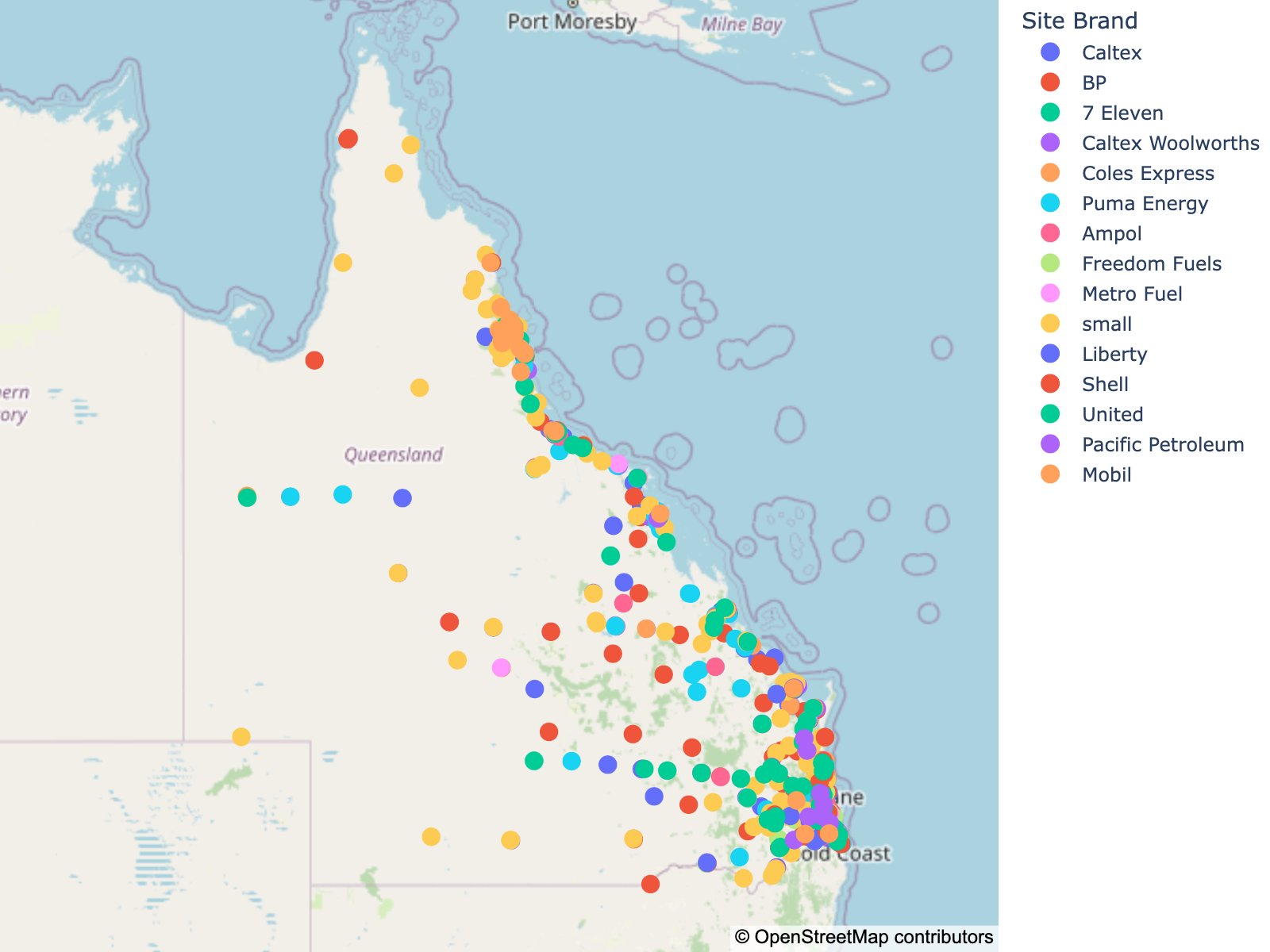
Figure 1: Queensland Fuel Stations

Figure 2 displays the locations of fuel stations in Brisbane, the capital city of Queensland, along with their respective brands. It is evident that many stations are situated close to one another, particularly in the municipal area.

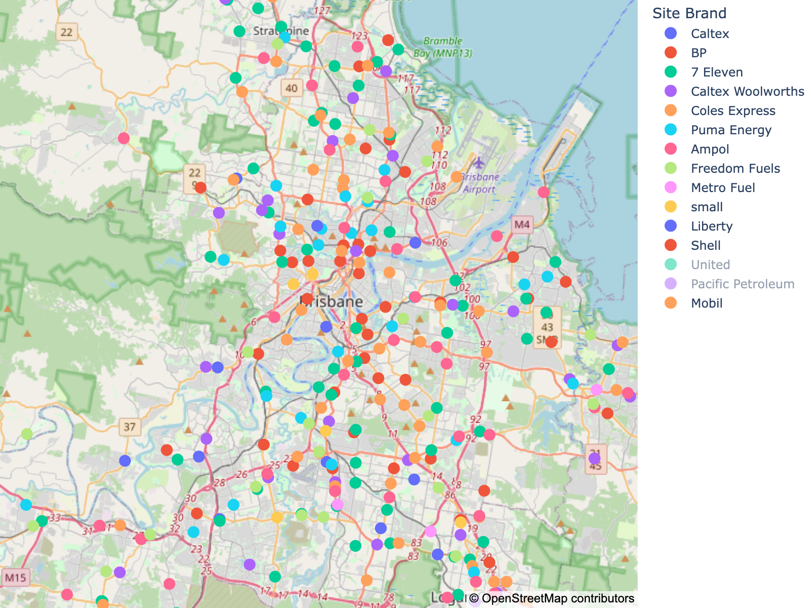
Figure 2: Brisbane (Queensland’s capital city) Fuel Stations

5.1 Data

We analyze unleaded gasoline, as in Pinkse et al. (2002), because it has the largest market share and is nearly a homogeneous product. Our data spans from February 1, 2019, to September 30, 2021, with a total of $T=973$ days and no missing values. This sample includes five lockdown periods in Queensland during the Covid-19 pandemic.

Figure 3 shows the average fuel prices for each brand over time, revealing clear seasonality. The significant drop in fuel prices in 2020 corresponds to the longest lockdown period, from March 26 to the end of April. Additionally, when aggregating over time, Figure 4 highlights the price heterogeneity across brands.

Figure 3: Average price by brands over time

The price unit is 1/10 cent per liter. Namely, 1200 means 1.2 Australian dollar per litre.

Figure 4: Average price by brands

In the following analysis, we exclude small brands with fewer than 5 stations and stations located on islands. After this cleaning process, we are left with $N=946$ stations. Throughout the sample period, no new stations were built, nor were any stations decommissioned. While some stations changed brands, we account for the brand effect in the estimation.

5.2 Empirical model specification and estimation

We apply the following empirical model in (1) to analyze the data.

$$Q_{y_{it}}\Big{(}\tau|X_{t},F_{t,\tau},B_{\tau},\Lambda_{\tau},\mbox{\boldmath$\rho$}_{\tau},\mbox{\boldmath$\gamma$}_{\tau},\mbox{\boldmath$\delta$}_{\tau}\Big{)}$$

$$\equiv\rho_{i,\tau}\sum_{i\neq j,j=1}^{N}w_{ij}Q_{y_{jt}}\Big{(}\tau|X_{t},F_{t,\tau},B_{\tau},\Lambda_{\tau},\mbox{\boldmath$\rho$}_{\tau},\mbox{\boldmath$\gamma$}_{\tau},\mbox{\boldmath$\delta$}_{\tau}\Big{)}$$

$$\quad+\delta_{i,\tau}\sum_{i\neq j,j=1}^{N}w_{ij}Q_{y_{j,t-1}}\Big{(}\tau|X_{t-1},F_{t-1,\tau},B_{\tau},\Lambda_{\tau},\mbox{\boldmath$\rho$}_{\tau},\mbox{\boldmath$\gamma$}_{\tau},\mbox{\boldmath$\delta$}_{\tau}\Big{)}$$

$$\quad+\gamma_{i,\tau}Q_{y_{i,t-1}}\Big{(}\tau|X_{t-1},F_{t-1,\tau},B_{\tau},\Lambda_{\tau},\mbox{\boldmath$\rho$}_{\tau},\mbox{\boldmath$\gamma$}_{\tau},\mbox{\boldmath$\delta$}_{\tau}\Big{)}+{\rm Covid}_{t}\times b_{{\rm covid},i,\tau}+{\rm Brand}_{it}\times b_{{\rm brand}_{it},\tau}$$

$$\quad+{\rm Year}_{t}\times b_{{\rm Year}_{it},\tau}+{\rm Month}_{t}\times b_{{\rm Month}_{it},\tau}+{\rm DayofWeek}_{t}\times b_{{\rm DayofWeek}_{it},\tau}+\sum_{k=1}^{r}f_{tk,\tau}\lambda_{ik,\tau}+G_{i,e_{it}}^{-1}(\tau)$$ (12)

In the above model, the subscript $i$ refers to fuel station $i$, and $t$ represents time (day). The independent variables in this model include several time effects: ${\rm Year}_{t}$, ${\rm Month}_{t}$, and ${\rm DayofWeek}_{t}$. The year effect captures any overall trend, while the month and day-of-the-week effects capture explicit seasonal variations. Each station $i$ has its own parameter for these time variables. For instance, the effect of the year 2021 differs for station 1 compared to station 2.

The brand ${\rm Brand}_{it}$ dummy variables capture the brand effect. Note that some stations changed brands during the sample period, which is why a double subscript is used for this variable. We include all brand dummy variables and exclude the intercept for identification purposes, so the station-specific effect is naturally incorporated.

The variable ${\rm Covid}_{t}$ is a dummy variable that takes the value 1 if time $t$ falls within a lockdown period and 0 otherwise. Details of the lockdown periods are provided in the appendix. Briefly, there was only one long lockdown period in 2020, from March 26 to the end of April, with all other periods being less than one week in duration.

For the weight matrix $W$, we consider driving distance rather than geographic distance, taking into account traffic conditions and speed limits in different areas. To compute the average driving time between two stations, we use the Open Source Routing Machine (OSRM). In this application, if two stations are within a 5-minute driving distance of each other, they are classified as neighbors. We normalize each row of the matrix $W$ such that the sum of the elements in each row equals 1. Specifically, if station 1 has three neighbors (stations 2, 7, and 9), then $W_{1,2}=W_{1,7}=W_{1,9}=\frac{1}{3}$, and all other $W_{1,j}=0$.

The prior is set to be informative but covers a broad range of the parameter space, as in the simulation. The detailed settings can be found in the appendix.

5.3 Results

Due to the large number of parameters in the model, such as the number of $\rho$, $\delta$, $\gamma$, and $b$, $\Lambda$, $F$, which totals $3N+N(p+1)+r_{f}(T+N)=44,597$ in our application, we do not store all simulated values during the MCMC process. Instead, we focus on the posterior means, which allows us to accumulate values with minimal memory usage. This approach makes it straightforward to evaluate uncertainties. For example, if posterior variance is required, we can save the sum of the squared values, then use the sample mean of the squared values and the sample mean to compute the sample variance. Any moment-based posterior statistics can be derived in this way.

Figure 5 presents the histogram of the posterior means of $\rho_{i,\tau}$ for all $i$ at the quantiles $\tau=(0.01,0.05,0.5,0.95,0.99)$. Without imposing any restrictions, the distribution of $\rho_{t,\tau}$ reveals two key characteristics. First, the values are positive, indicating that positive spillover effects exist between fuel prices at nearby stations. Second, the heterogeneity patterns are consistent across different quantiles. Some stations exhibit greater sensitivity to their neighbors (larger $\rho$ values), while others show minimal sensitivity, with $\rho$ values close to zero. Figure 5 underscores the need for a heterogeneous coefficient model.

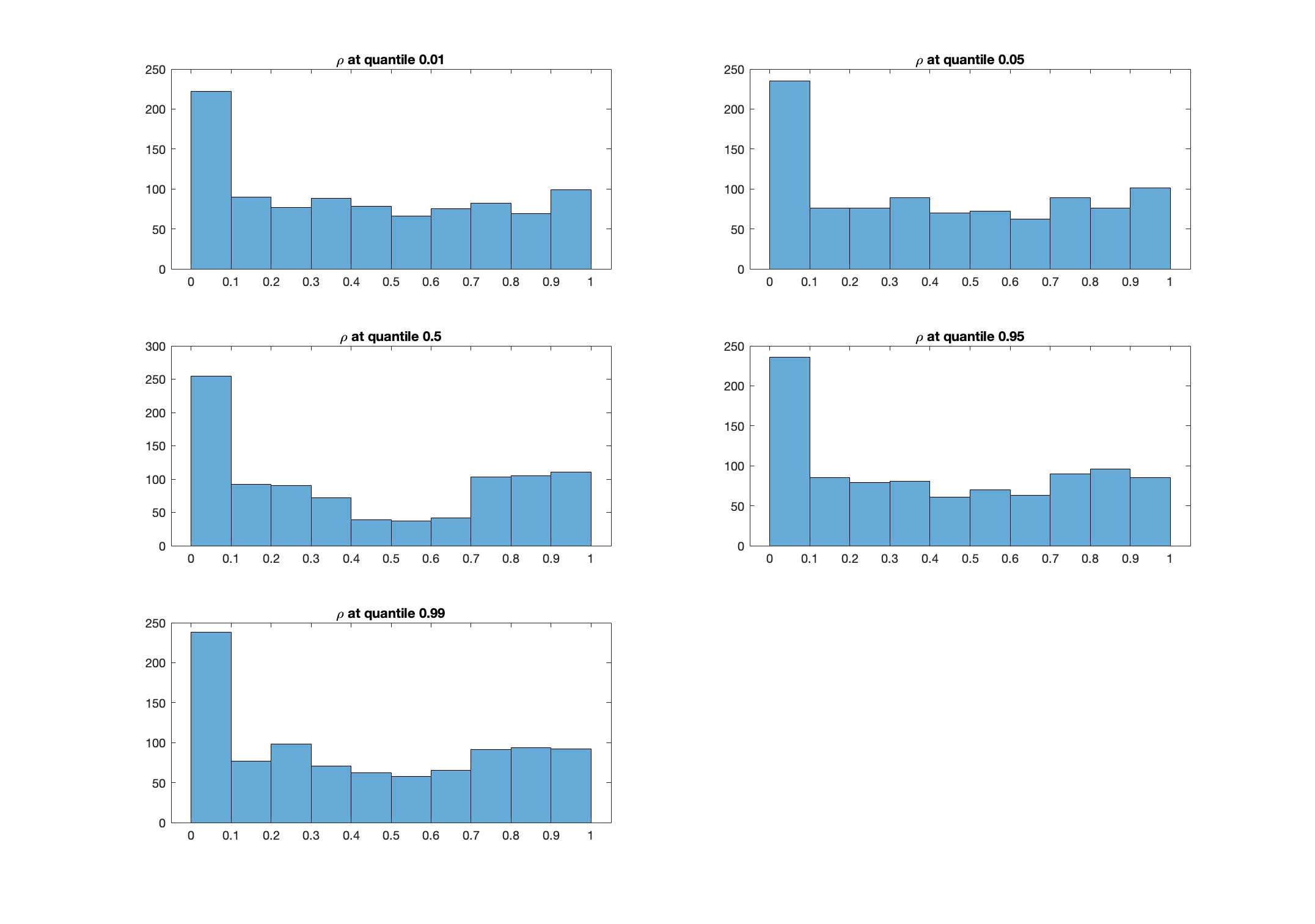
Figure 5: Distributions of $\rho$

Figure 6 shows the distribution of the posterior means of the Covid lockdown coefficients at different quantiles. It is clear that the distributions of these coefficients differ significantly across quantiles. For instance, the histogram for $\tau=0.05$ is right-skewed, while the histogram for $\tau=0.99$ is left-skewed. The mode is around zero. This is not surprising, as the factors are intended to capture any systematic price changes. Figure 6 demonstrates that the lockdowns have caused changes in prices, not only in terms of dispersion but also in how these price responses vary across different quantiles.

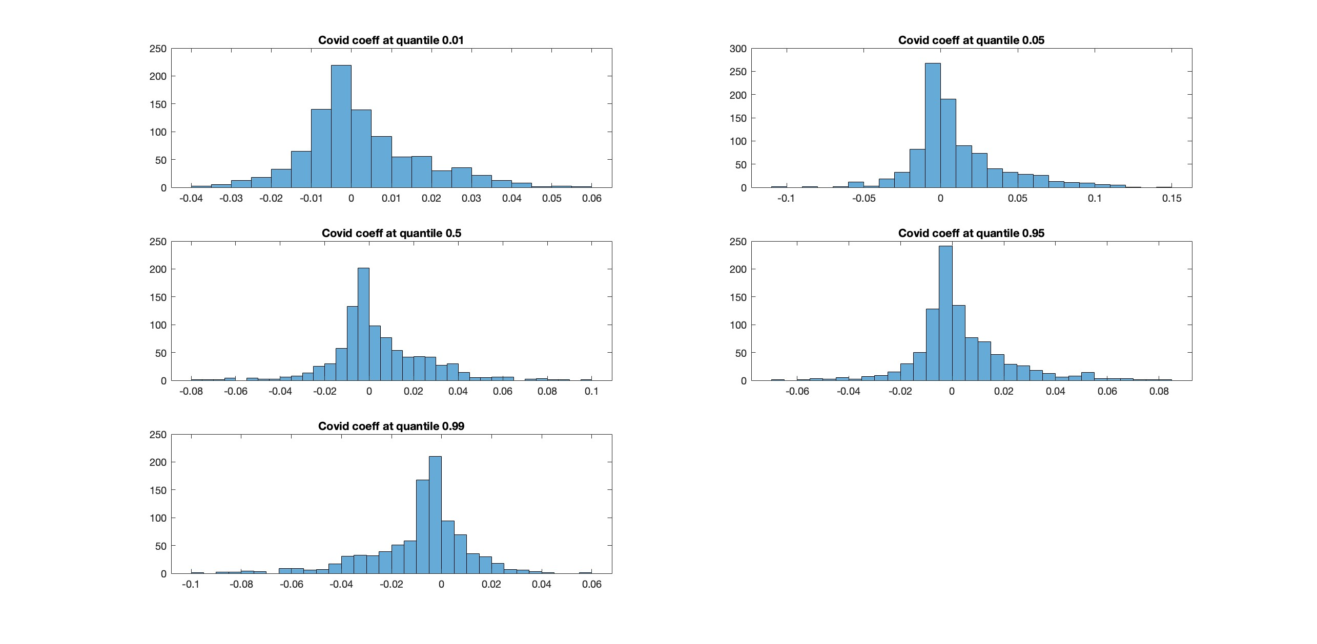
Figure 6: Distribution of Covid Coefficients

Figure 7 displays the average brand premiums across different quantiles. It is important to note that each station has its own distinct brand premium, which can be interpreted as the average station effect within the same brand. Similar patterns emerge across the brand premiums. For instance, Pacific Petroleum consistently has the lowest values, while United Petroleum consistently has the highest values across all quantiles.

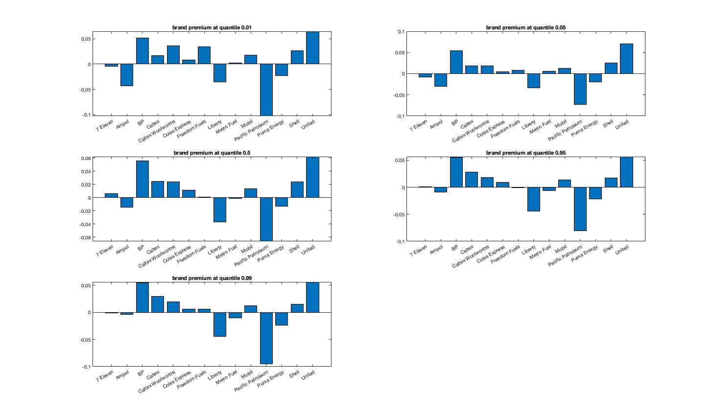
Figure 7: Average Brand Premiums

Similar to the spatial coefficient $\rho_{i,\tau}$, the lag coefficient $\gamma_{i,\tau}$ and the lag-spatial coefficient $\delta_{i,\tau}$ demonstrate a strong pattern of heterogeneity, while exhibiting similar patterns across quantiles, respectively. Due to page limitations, these are not shown here.

The systemic factors and their effects on each time series are plotted in Figure 8. Each subplot represents $N=946$ time series, depicting $\mathbf{\lambda}_{i,\tau}^{\prime}\mathbf{f}_{t,\tau}$. It is evident that the factor structure captures the seasonality present in the data. Since the simulation study does not indicate the correct number of factors, we refrain from analyzing individual factors in this application.

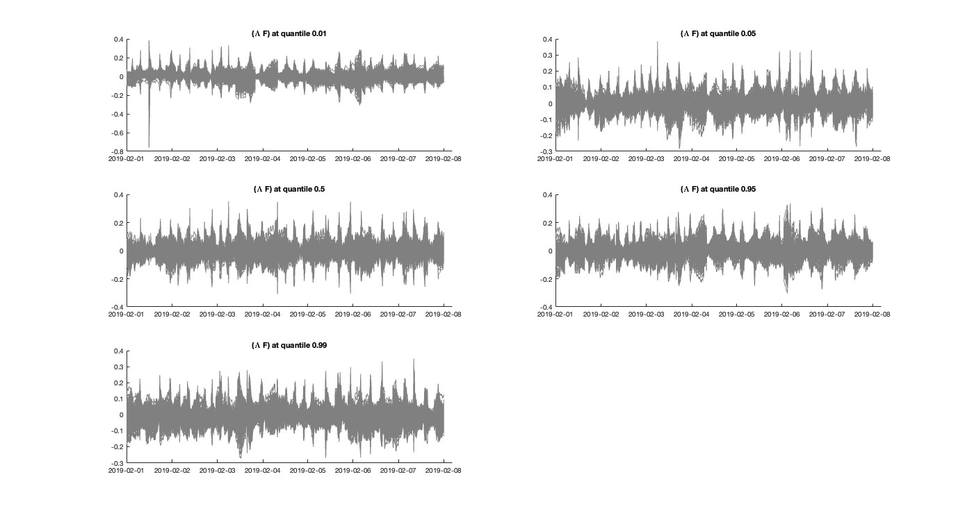
Figure 8: Posterior mean of $\Lambda F$

We compute the average variation from the posterior mean of the contemporaneous effect. Specifically, we consider the term $\rho_{i,\tau}\sum_{i\neq j,j=1}^{N}w_{ij}Q_{y_{jt}}\left(\tau|X_{t},F_{t,\tau},B_{\tau},\Lambda_{\tau},\mbox{\boldmath$\rho$}_{\tau},\mbox{\boldmath$\gamma$}_{\tau},\mbox{\boldmath$\delta$}_{\tau}\right)$ from equation (12). The ratio of the average variation of this term to the average variation of the posterior values of the quantiles is approximately $30\%$ for all quantiles in $(0.01,0.05,0.5,0.95,0.99)$. This suggests that the contemporaneous spatial effect plays a significant role in explaining the quantiles.

6 Conclusion

In this paper, we introduced a novel dynamic spatial panel quantile model with interactive effects. The model is capable of simultaneously addressing multiple features, including spatial effects (spillover effects), heterogeneous regression coefficients, and unobservable heterogeneity that vary across quantiles. To estimate this model, we proposed a new Bayesian estimation procedure, and we established Bayesian consistency to justify the method. We applied the proposed model and method to analyze gasoline price data in Australia.

Recently, Ando et al. (2024) developed a scenario-based quantile network connectedness framework that accommodates various economic scenarios. This is achieved through a scenario-based moving average representation of the model, where forecast error variance decomposition is conducted under pre-specified future scenarios. In a similar vein, the expression in (3) allows for the implementation of scenario-based quantile network connectedness. This represents an interesting direction for future research.

Supplementary Materials

All technical proofs of theoretical results and some numerical results are delegated to the supplementary document.

References

- Ando and Bai (2017) Ando, T. and J. Bai (2017). Clustering huge number of financial time series: A panel data approach with high-dimensional predictors and factor structures. Journal of the American Statistical Association 112(519), 1182–1198.
- Ando and Bai (2020) Ando, T. and J. Bai (2020). Quantile co-movement in financial markets: A panel quantile model with unobserved heterogeneity. Journal of the American Statistical Association 115(529), 266–279.
- Ando et al. (2024) Ando, T., J. Bai, L. Lu, and C. Vojtech (2024). Scenario-based quantile connectedness of the u.s. interbank liquidity risk network. Journal of Econometrics 244(2), 105786.
- Ando et al. (2023) Ando, T., K. Li, and L. Lu (2023). A spatial panel quantile model with unobserved heterogeneity. Journal of Econometrics 232(1), 191–213.
- Aquaro et al. (2021) Aquaro, M., N. Bailey, and M. H. Pesaran (2021). Estimation and inference for spatial models with heterogeneous coefficients: an application to us house prices. Journal of Applied Econometrics 36(1), 18–44.
- Bai (2009) Bai, J. (2009). Panel data models with interactive fixed effects. Econometrica 77(4), 1229–1279.
- Bai and Li (2012) Bai, J. and K. Li (2012). Statistical analysis of factor models of high dimension. The Annals of Statistics 40(1), 436–465.
- Bai and Li (2013) Bai, J. and K. Li (2013). Spatial panel data models with common shocks. manuscript.
- Bai and Li (2021) Bai, J. and K. Li (2021). Dynamic spatial panel data models with common shocks. Journal of Econometrics 224(1), 134–160.
- Bai and Liao (2016) Bai, J. and Y. Liao (2016). Efficient estimation of approximate factor models via penalized maximum likelihood. Journal of econometrics 191(1), 1–18.
- Bai and Ng (2002) Bai, J. and S. Ng (2002). Determining the number of factors in approximate factor models. Econometrica 70(1), 191–221.
- Bai and Ng (2013) Bai, J. and S. Ng (2013). Principal components estimation and identification of static factors. Journal of econometrics 176(1), 18–29.
- Baltagi (2011) Baltagi, B. (2011). Spatial Panels, Chapter 15, pp. 435–454. Chapman and Hall.
- Barron et al. (1999) Barron, A., M. J. Schervish, and L. Wasserman (1999). The consistency of posterior distributions in nonparametric problems. Annals of Statistics 27, 536–561.
- Beenstock and Felsenstein (2015) Beenstock, M. and D. Felsenstein (2015). Estimating spatial spillover in housing construction with nonstationary panel data. Journal of Housing Economics 28, 42–58.
- Chen et al. (2021) Chen, L., J. Gonzalo, and J. Dolado (2021). Quantile factor models. Econometrica 89, 875–910.
- Chhikara (1988) Chhikara, R. (1988). The Inverse Gaussian Distribution: Theory, Methodology, and Applications. CRC Press.
- Ghosal et al. (1999) Ghosal, S., J. K. Ghosh, and R. V. Ramamoorthi (1999). Posterior consistency of dirichlet mixtures in density estimation. Annals of Statistics 27, 143–158.
- Glaser et al. (2022) Glaser, S., R. Jung, and K. Schweikert (2022). Spatial panel count data: modeling and forecasting of urban crimes. Journal of Spatial Econometrics 3(2).
- Green (1995) Green, P. J. (1995). Reversible jump markov chain monte carlo computation and bayesian model determination. Biometrika 82(4), 711–732.
- Hallin and Lika (2007) Hallin, M. and R. Lika (2007). The generalized dynamic factor model: determining the number of factors. Journal of the American Statistical Association 102, 603–617.
- Harding et al. (2020) Harding, M., C. Lamarche, and M. Pesaran (2020). Common correlated effects estimation of heterogeneous dynamic panel quantile regression models. Journal of Applied Econometrics 35(3), 294–314.
- Hunneman et al. (2022) Hunneman, A., J. Elhorst, and T. Bijmolt (2022). Store sales evaluation and prediction using spatial panel data models of sales components. Spatial Economic Analysis 17, 127–150.
- Kelejian and Prucha (2004) Kelejian, H. H. and I. R. Prucha (2004). Estimation of simultaneous systems of spatially interrelated cross sectional equations. Journal of Econometrics 118, 27–50.
- Koenker and Bassett (1978) Koenker, R. and G. Bassett (1978). Regression quantiles. Econometrica 46, 33–50.
- Koenker and Xiao (2006) Koenker, R. and Z. Xiao (2006). Quantile autoregression. Journal of the American Statistical Association 101(9), 980–990.
- Lee (2004) Lee, L. (2004). Asymptotic distributions of quasi-maximum likelihood estimator for spatial autoregressive models. Econometrica 72(6), 1899–1925.
- Li (2017) Li, K. (2017). Fixed-effects dynamic spatial panel data models and impulse response analysis. Journal of Econometrics 198(1), 102–121.
- Lin and Lee (2010) Lin, X. and L. Lee (2010). Gmm estimation of spatial autoregressive models with unknown heteroscedasticity. Journal of Econometrics 157, 34–52.
- Lu (2017) Lu, L. (2017). Simultaneous spatial panel data models with common shocks. RPA working paper RPA17-03, Federal Reserve Bank of Boston.
- Lu and Su (2016) Lu, X. and L. Su (2016). Shrinkage estimation of dynamic panel data models with interactive fixed effects. Journal of Econometrics 190(1), 148–175.
- Malsiner-Walli et al. (2016) Malsiner-Walli, G., S. Frühwirth-Schnatter, and B. Grün (2016). Model-based clustering based on sparse finite gaussian mixtures. Statistics and computing 26(1-2), 303–324.
- Mitchell and Beauchamp (1988) Mitchell, T. J. and J. J. Beauchamp (1988). Bayesian variable selection in linear regression. Journal of the american statistical association 83(404), 1023–1032.
- Moon and Weidner (2015) Moon, H. R. and M. Weidner (2015). Linear regression for panel with unknown number of factors as interactive fixed effects. Econometrica 83, 1543–1579.
- Pesaran (2006) Pesaran, M. (2006). Estimation and inference in large heterogeneous panels with a multifactor error structure. Econometrica 74(4), 967–1012.
- Pinkse et al. (2002) Pinkse, J., M. E. Slade, and C. Brett (2002). Spatial price competition: a semiparametric approach. Econometrica 70(3), 1111–1153.
- Qu and Lee (2015) Qu, X. and L. Lee (2015). Estimating a spatial autoregressive model with an endogenous spatial weight matrix. Journal of Econometrics 184(2), 209–232.
- Reich et al. (2011) Reich, B. J., M. Fuentes, and D. B. Dunson (2011). Bayesian spatial quantile regression. Journal of the American Statistical Association 106(493), 6–20.
- Shi and Lee (2017) Shi, W. and L. Lee (2017). Spatial dynamic panel data models with interactive fixed effects. Journal of Econometrics 197, 323–347.
- Stock and Watson (2002) Stock, J. and M. Watson (2002). Forecasting using principal components from a large number of predictors. Journal of the American Statistical Association 97, 1167–1179.
- Villani (2009) Villani, M. (2009). Steady-state priors for vector autoregressions. Journal of Applied Econometrics 24(4), 630–650.
- Walker and Hjort (2001) Walker, S. G. and N. L. Hjort (2001). On bayesian consistency. Journal of the Royal Statistical Society: Series B 63, 811–821.
- Yu et al. (2008) Yu, J., R. de Jong, and L. Lee (2008). Quasi-maximum likelihood estimators for spatial dynamic panel data with fixed effects when both and are large. Journal of Econometrics 146(1), 118–134.