Riemann Tensor Neural Networks: Learning Conservative Systems with Physics-Constrained Networks
Abstract
Divergence-free symmetric tensors (DFSTs) are fundamental in continuum mechanics, encoding conservation laws such as mass and momentum conservation. We introduce Riemann Tensor Neural Networks (RTNNs), a novel neural architecture that inherently satisfies the DFST condition to machine precision, providing a strong inductive bias for enforcing these conservation laws. We prove that RTNNs can approximate any sufficiently smooth DFST with arbitrary precision and demonstrate their effectiveness as surrogates for conservative PDEs, achieving improved accuracy across benchmarks. This work is the first to use DFSTs as an inductive bias in neural PDE surrogates and to explicitly enforce the conservation of both mass and momentum within a physics-constrained neural architecture.
1 Introduction
Partial Differential Equations (PDEs)
Partial Differential Equations (PDEs) are central to the mathematical modeling of complex physical systems, including fluid dynamics, thermodynamics, and material sciences. Traditional numerical methods, such as finite element and spectral methods, often require fine discretization of the physical domain to achieve high accuracy. These approaches can become computationally expensive, particularly in engineering applications where systems must be solved repeatedly under varying parameters or initial conditions. Recent advances in machine learning (ML) have shown promise in addressing these challenges by leveraging neural networks (NNs) as potential alternatives or enhancements to traditional numerical solvers (Kovachki et al., 2021; Li et al., 2020).
Physical Inductive Biases in Machine Learning.
A central limitation of generic neural models is their lack of built-in physical intuition. While convolutional or attention-based layers successfully exploit certain data symmetries (e.g., translation invariance), they do not automatically enforce fundamental physics, such as mass conservation or energy preservation. Physics-Informed Neural Networks (PINNs) (Lagaris et al., 1998; Raissi et al., 2019b; Cai et al., 2021; Haghighat et al., 2021; Hu et al., 2023) address this gap by adding PDE residuals and boundary conditions as soft constraints in the loss function. PINNs have been successfully deployed on many PDE problems (Karniadakis et al., 2021; Jnini et al., 2024b), but the “soft penalty” approach can lead to suboptimal enforcement of conservation laws and stiff optimization (Wang et al., 2021). Consequently, there is growing interest in hard or explicit constraints that guarantee PDE structure a priori (Richter-Powell et al., 2022; Greydanus et al., 2019b; Jnini et al., 2024a).
Divergence-Free Symmetric Tensors in Physics and Mathematics.
Divergence-free symmetric tensors (DFSTs) are a special class of tensor fields characterized by vanishing row-wise divergence and inherent symmetry in their indices. In an -dimensional space-time domain, where represents the spatial dimensions and the additional dimension accounts for time, these tensors frequently arise as stress or momentum flux tensors in various fields, including fluid dynamics, elasticity, kinetic theory, and relativistic hydrodynamics (Serre, 2018). For instance, the Navier–Stokes stress tensor or the compressible flux matrix can be represented as an tensor satisfying . This formulation unifies the conservation of mass and momentum under a single flux-divergence constraint. Despite their natural alignment with PDE-based conservation laws, existing studies have not explored leveraging DFST structures directly as a neural inductive bias within neural network architectures.
Our Contributions.
In this work, we present a novel approach to embedding fundamental conservation laws directly into neural network architectures through DFSTs . Our primary contributions are as follows:
-
1.
Architectural Design of Riemann Tensor Neural Networks (RTNNs) : We introduce RTNNs , a class of neural architectures specifically designed to generate DFST fields. RTNNs are tailored for approximating individual DFSTs, ensuring the divergence-free condition, , is satisfied to machine precision.
-
2.
Theoretical Guarantees for RTNNs: We establish theoretical foundations for RTNNs by proving their universal approximation capabilities for any sufficiently smooth DFST.
-
3.
Empirical Validation and Comparative Analysis: We reformulate several benchmark problems within the DFST framework and conduct numerical experiments that demonstrate RTNNs consistently improve performance of PINNs in accuracy when used as surrogate models for conservative PDEs.
In the following sections, we review DFST-based PDE formulations, describe the proposed neural architectures, and present experimental validations on benchmark problems.
1.1 Related works
Divergence-Free Symmetric Tensors in Mathematical Physics.
A large body of work by (Serre, 1997, 2018, 2019, 2021) has established the fundamental importance of DFSTs in continuum mechanics and kinetic theory. These tensors encode conservation principles for mass and momentum (in classical fluid dynamics) or energy–momentum (in relativistic hydrodynamics), and are present in models ranging from Euler or Boltzmann equations to mean-field (Vlasov–Poisson) descriptions of plasmas and galaxies. Although DFSTs have been investigated in PDE theory, prior investigations have largely focused on analytic or qualitative properties . To the best of our knowledge, no existing work leverages DFSTs explicitly as a numerical method or as an architectural inductive bias in machine learning frameworks.
Hard-Constraints in Scientific Machine Learning.
Beyond the classical physics-informed approach of adding PDE residuals as soft constraints in the loss (Raissi et al., 2019a; Karniadakis et al., 2021), there is growing interest in incorporating hard constraints or specialized structures into neural networks. For instance, (Hendriks et al., 2020) investigate linearly constrained networks, (Richter-Powell et al., 2022) impose continuity-equation constraints via divergence-free vector fields, and several recent methods aim to preserve energy or momentum (Greydanus et al., 2019a). These efforts reflect a broader push in machine learning to embed domain-specific priors, thereby improving stability and generalization (LeCun et al., 1998; Giles & Maxwell, 1987). Our work similarly encodes the PDE structure “at the network level” via DFST, which ensures strict conservation and symmetry. To the best of our knowledge, this work is the first to use enforce the conservation of both mass and momentum at the architectural level for surrogate modeling.
2 Background and Theory
Notation (Preliminaries)
Let denote the spatial dimension and the spatial domain. The space-time domain is , where and . For a function , the augmented gradient is , and the spatial gradient is .
Divergence-Free Symmetric Tensors in Continuum Mechanics.
We begin by introducing the class of divergence-free symmetric tensors, which encode either the conservation of mass and momentum in classical mechanics or energy and momentum in special relativity. A tensor field
is said to be symmetric if , and divergence-free if it satisfies
Many classical PDE systems, including compressible or incompressible fluid flow, elasticity, and shallow-water models, can be expressed in this flux-divergence form by suitably choosing . A canonical representation in fluid mechanics is:
| (1) |
where denotes the mass density, the linear momentum field, and the stress tensor. Enforcing then unifies mass and momentum conservation, while additional constraints (e.g., constitutive laws or energy equations) can further specify or couple and .
Motivation for Neural Parametrization.
Although one can penalize the residuals of the condition in a soft-constraint manner (e.g., through terms in the loss function), this approach does not guarantee the satisfaction of the divergence-free condition, especially when optimization is challenging or regularization terms are underweighted, this is often the case in the non-linear regime that we are considering, as describe in (Bonfanti et al., 2024). Instead, we propose embedding the divergence-free property directly into the neural network architecture. This hard-coded constraint ensures strict conservation to machine precision, providing better stability and physical consistency.
Proposed Approach.
The following sections introduce a neural-network-based construction that guarantee the output is a divergence-free symmetric tensor. We prove that our approach can approximate any sufficiently smooth DFST to arbitrary accuracy, thus offering a robust way to integrate conservation principles into neural PDE solvers.
2.1 Constructing Divergence-Free Symmetric Tensors on a Flat Manifold (DFSTs)
Theorem 2.1 (Representation of Divergence-Free Symmetric Tensors on a Flat Manifold).
Let be an -dimensional real vector space with a fixed basis , and let denote the corresponding dual basis of . Let denote the space of 2-forms on . Consider the space of all -tensors defined on a flat manifold equipped with a Levi-Civita connection , satisfying the following symmetries:
-
1.
Antisymmetry within index pairs:
(2) (3) -
2.
Symmetry between pairs:
(4)
Let be a fixed basis of , where . Define the tensors:
| (5) |
where is the wedge product of the dual basis elements and .
Proof.
The proof is presented in Appendix A. ∎
2.2 Riemann Tensor Neural Network
In the setting where we wish to approximate a divergence-free symmetric tensor field
| (8) |
we define a Riemann Tensor Neural Network as follows.
Definition 2.2 (Riemann Tensor Neural Network111So named because the underlying -tensors share index symmetries with the Riemann curvature tensor in differential geometry.).
Suppose:
-
•
is a flat domain (manifold without boundary or with suitable BCs),
-
•
is a finite non-trainable basis of Riemann-like -tensors as defined in Theorem 2.1,
-
•
is a multilayer perceptron (MLP) with twice-differentiable activations, whose input indexes points in .
Then an RTNN for the single-field case is constructed by:
-
1.
Scalar coefficients : The MLP outputs scalar functions .
-
2.
Hessian Computation: For each , compute the Hessian components via automatic differentiation.
-
3.
Tensor Field Construction: Define the -tensor field
(9) By design, is row-wise divergence-free and symmetric for all .
We call a Riemann Tensor Neural Network. It provides a parametric approximation to a single DFST on .
Remark 2.3.
Although the network outputs scale as , the problem setup is generally overparameterized. Depending on the application, certain scalar functions can be set to zero without violating the DSFT condition, provided that the number of basis functions exceeds the degrees of freedom.
2.3 Universal Approximation Theorem for RTNN
Theorem 2.4 (Universal Approximation for RTNN).
Let be a bounded (hence compact) domain, and suppose is a -smooth, divergence-free, symmetric tensor field on . Then for any , there exists a Riemann Tensor Neural Network such that
| (10) |
where denotes the Frobenius norm on . In particular, also remains divergence-free and symmetric on .
Proof.
We present the proof in Appendix A.3 ∎
3 Methodology and Applications
The preceding sections established the theoretical foundation of divergence-free symmetric tensors DFSTs and RTNNs as a rigorous approach to enforcing conservation laws within neural architectures. In the following section, we move from theory to application, showcasing how RTNNs can be employed to model various conservative systems, including the Euler and Navier-Stokes equations, and Magneto-Hydrodynamics(MHD).
3.1 Efficient Implementation and Practical Considerations
Automatic Differentiation
We employ Taylor-Mode Automatic Differentiation, which propagates Taylor coefficients through the network by treating the computational graph as an augmented network with weight sharing. This approach effectively reduces redundant computations associated with higher-order derivatives, significantly accelerating the training process of RTNNs. Additionally, for Magneto-Hydrodynamics in Section 3.4, we utilize Separable Physics-Informed Neural Networks (SPINNs). SPINNs decompose PDE residuals into per-axis evaluations, facilitating efficient differential operations on large-scale regular grids (Cho et al., 2023).
Optimization and Stability
Our method models densities and momenta instead of velocity fields, velocity recovery involves dividing by , leading to instability when is initialized around a small value (Richter-Powell et al., 2022). To address this, we add an identity matrix to , ensuring is initialized near 1 without violating DFST constraints. Throughout the experiments in this paper, we use the Least-memory BFGS (Nocedal & Wright, 1999) optimizer due to the highly non-linear nature of our problems. Additionally, LBFGS efficiently approximates second-order curvature information, facilitating effective optimization in the complex, non-linear loss landscapes encountered in our experiments. The challenges of optimizing in such regimes and the importance of second-order optimizers have been well documented in the literature (Jnini et al., 2024b; Müller & Zeinhofer, 2023, 2024; Bonfanti et al., 2024).
Code implementation and public repository
Our code has been implemented using the JAX library (Bradbury et al., 2018). Code and experiments will be publicly released upon acceptance.
3.2 Pedagogic Example: 2D Isentropic Euler Vortex
For this pedagogic example, we simulate a 2D isentropic Euler vortex—a smooth, rotational flow solution to the Euler equations that accurately captures vortex dynamics and is commonly used as a standard benchmark for evaluating the accuracy of numerical solvers—over a spatial domain and a time interval . We employ well-defined analytical initial and boundary conditions that are detailed in Appendix B.1.
Let denote the density, the velocity field, and the pressure. For isentropic flow with , the pressure is given by . The governing equations, including the energy equation, are:
Governing Equations.
The 2D compressible Euler equations are:
| (11) | |||
| (12) | |||
| (13) | |||
| (14) |
where is the total energy.
DFST Formulation and Decomposition of .
Rewriting (11)–(13) in flux-divergence form, we express the system as:
Here, the stress tensor is:
where represents the isotropic pressure contribution. The absence of a deviatoric term reflects the assumption of inviscid flow. The divergence-free condition enforces:
-
•
mass conservation, and
-
•
momentum conservation in - and -directions.
Additionally, the energy equation is given separately as:
where the total energy is:
RTNN Parametrization.
To approximate solutions of (11)–(14), we define a family of tensors using RTNNs . The parametrization proceeds as follows:
-
1.
RTNN Parametrization of : Let denote an RTNN as described in Section 2.2. By construction, is divergence-free and symmetric in .
-
2.
Extracting Physical Fields: We can interpret in block form. From it, we read off::
-
3.
Zero-Deviatoric Constraint and Energy Parametrization: We can parametrize the pressure decomposing the stress tensor into isotropic and deviatoric parts:
where:
(15) Additionally, we parametrize the energy as:
For an inviscid isentropic vortex, we enforce the constraint during training.
While the parametrized fields exactly satisfy the DSFT constraints, they only are solutions to the momentum equations if the stress tensor satisfies the zero deviatoric constraints, which we can penalize in the loss function in addition to the boundary and initial terms.
Loss Function.
To train the RTNN and ensure that the modeled tensor adheres to the governing equations and boundary conditions, we define an objective function:
where penalizes deviations from the prescribed boundary conditions while enforces consistency with initial conditions. The term ensures that the stress tensor remains purely isotropic by penalizing the magnitude of the deviatoric component, . Finally, minimizes the residual of the energy equation, measured as , ensuring that the total energy is properly conserved within the system. Additionally, incorporates supervised learning by penalizing the discrepancies between the model predictions and observed data labels. All loss terms are formulated in the least squares sense.
Experimental Setup.
For the neural network training, we sample 500 interior collocation points within to enforce the residual constraints of the governing PDE. Additionally, 100 boundary and initial condition points are sampled to impose the prescribed constraints. Our RTNN model is parameterized by a Multilayer Perceptron (MLP) with 4 hidden layers, each containing 50 neurons. Training is performed entirely without labeled data,the model is validated against the analytical solution of the isentropic Euler vortex to evaluate accuracy.
We benchmark RTNN against two methods: (1) the standard PINN approach and (2) Neural Conservation Laws (NCL) that enforces exact mass conservation(Richter-Powell et al., 2022). Both methods use similar MLP architectures for fairness. Performance is evaluated in terms of median average relative error on all fields and simulation time. We train all three methods using 200,000 iterations of the L-BFGS optimizer. We follow the loss scheme presented in this section, while training both PINN and NCL using PDE residuals penalized in the loss.
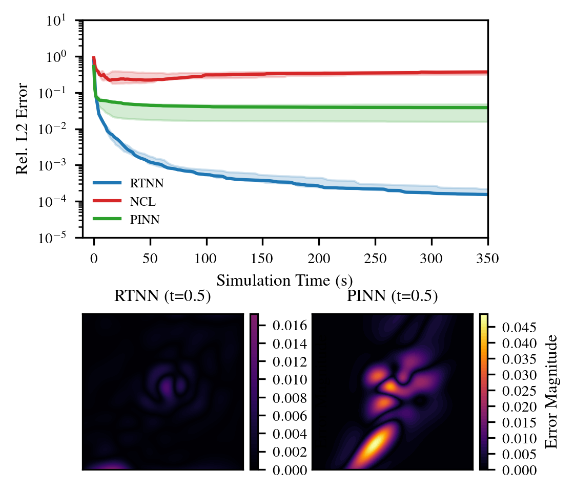
Results and Discussion.
Table 1 summarizes the results, while Figure 1 presents the evolution of the relative error over simulation time. Our RTNN significantly outperforms both PINN and NCL, achieving a median relative error that is two orders of magnitude lower than PINN and four orders of magnitude lower than NCL. Furthermore, RTNN demonstrates stable convergence while maintaining competitive training times.
| Method | Relative Error | Wall Time (s) |
|---|---|---|
| RTNN | 9.92e-05 | 596.34 |
| NCL | 3.87e-01 | 2008.57 |
| PINN | 3.82e-02 | 365.67 |
3.3 Incompressible Navier-Stokes Equation
We next consider the incompressible Navier-Stokes equations, which include additional viscous forces compared to inviscid Euler flows.
Governing Equations.
The incompressible Navier-Stokes system in the -dimensional case is given by:
| (16) | ||||
| (17) |
where represents the velocity field, denotes the pressure field, and is the kinematic viscosity. Equation (16) enforces the incompressibility condition, ensuring that the divergence of the velocity field is zero. Meanwhile, equation (17) balances the convective, pressure, and viscous forces within the fluid. The term specifically models the internal fluid friction due to viscosity.
DFST Formulation and Stress Decomposition.
These equations can be expressed in a divergence-free symmetric tensor (DFST) form. We define a tensor
such that
Here, the term represents the convective flux, while is the total stress tensor decomposed as
where the deviatoric part captures viscous stresses via
Exact incompressibility.
To enforce exact incompressibility (i.e., ), observe that any contributions to come specifically from basis 2-forms containing . Consequently, by choosing the corresponding coefficients to vanish whenever the wedge product includes in , we ensure that consists only of the identity term we added for stability, thus achieving exact incompressibility.
RTNN Parametrization.
Following Section 3.2, we employ an RTNN to represent the solution. From its block structure, we extract the physical fields as:
Here, represents the density field, while correspond to the velocity components. The viscous stress tensor can be computed via automatic differentiation applied directly to the velocity field. Instead, we define:
Although this introduces additional computational complexity, it can be mitigated using Taylor-mode automatic differentiation. The stress tensor can decomposed into an isotropic part and a deviatoric part:
Viscous Residual and Loss Function.
To enforce momentum balance, we focus on matching the RTNN-derived deviatoric stress with the velocity-based viscous stress . Define:
Because pressure can act as a scalar offset in this formulation, ensuring correct deviatoric stresses is sufficient to satisfy the momentum equation. Consequently, our training objective can be written:
where and enforce boundary and initial conditions, and penalizes any available labeled measurements. All loss terms are formulated in the least squares sense.
Experimental Setups.
We validate our approach on three representative incompressible Navier–Stokes scenarios:
-
•
3D Beltrami Flow We consider the three-dimensional Beltrami flow at a Reynolds number of to verify the accuracy of our RTNN framework. The computational domain is discretized using 2,601 interior collocation points to enforce the PDE residuals, supplemented by 961 boundary and initial condition points to impose the necessary constraints. An MLP with 4 hidden layers and 50 neurons per layer employing Tanh activation functions is utilized. The model is trained using 100,000 iterations of the L-BFGS optimizer without any labeled data. Validation is performed against 26,000 interior points sampled within the domain to assess the model’s performance. Detailed setup information and error plots are provided in Section B.2.
-
•
Steady Flow around a NACA Airfoil This experiment investigates the steady laminar flow at around a NACA 0012 airfoil. The steady-state problem is addressed by treating time as a dummy dimension set to zero in the forward pass. The computational domain is discretized with 40,000 collocation points to enforce PDE residuals and boundary conditions, alongside 2,000 labeled data points obtained from an in-house Reynolds-Averaged Navier-Stokes (RANS) solver to supervise the training. An MLP consisting of 4 hidden layers and 50 neurons per layer with Tanh activation functions is employed. The model undergoes 50,000 iterations of the L-BFGS optimizer. Validation is conducted on the 14,000 collocation points to evaluate accuracy. Further setup details and visual results are provided in Section B.4.
-
•
Cylinder Wake We simulate a two-dimensional unsteady vortex-shedding flow at around a circular cylinder centered at . The computational domain is defined as with the time interval , discretized in increments of . The domain is discretized using 40,000 interior collocation points to enforce the PDE residuals and 5,000 boundary and initial condition points to apply the necessary constraints. A 4-layer, 50-neuron MLP with Tanh activation functions is trained using 50,000 iterations of the L-BFGS optimizer without any labeled data. Validation is performed using Direct Numerical Simulation (DNS) data from Raissi et al. (2019a) to assess the model’s performance. Comprehensive setup details and error analyses are presented in Section B.3.
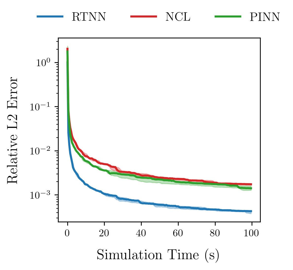
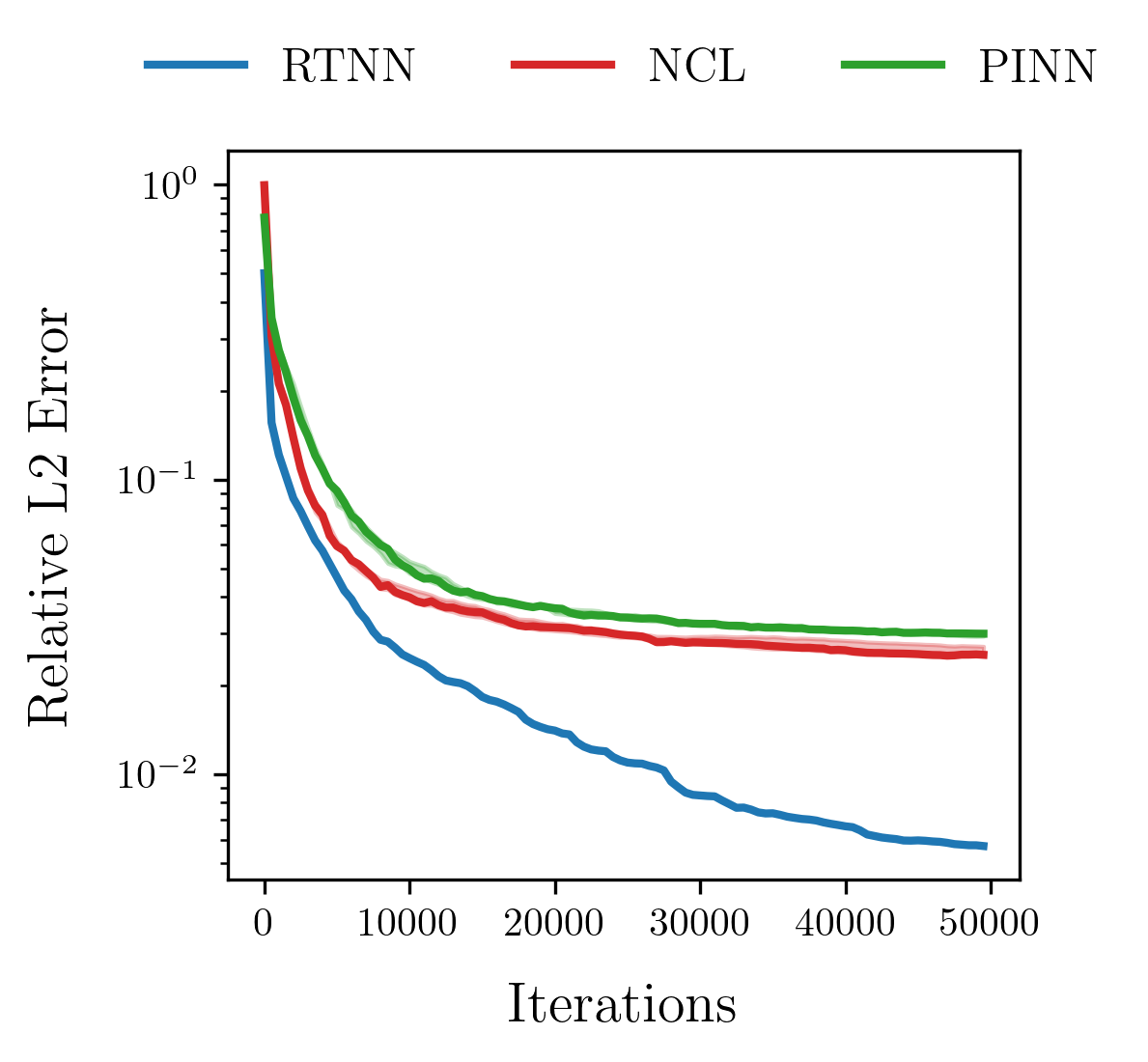
Results and Discussion.
Table 2 summarize the performance of our RTNN formulation compared to NCL and standard PINNs by showing median average relative error accross all fields and wall times, while Figures 4, 3 and 2 summarize the training dynamics for each experiment. As observed in the table, our ansatz delivers improved accuracy while achieving comparable training times.
Across all three test cases, the RTNN approach consistently yields lower relative errors, indicating its potential for robust, data-efficient modeling of incompressible Navier–Stokes flows for both self-supervised learning in the PINN manner and in in scarce-data scenarios.
| Cylinder | Airfoil | Beltrami | ||||
| Method | rL2 Error | Time (s) | rL2 Error | Time (s) | rL2 Error | Time (s) |
| RTNN | 5.70e-03 | 1.21e+03 | 1.44e-02 | 1.10e+03 | 4.28e-04 | 2.97e+02 |
| NCL | 2.54e-02 | 2.46e+03 | 1.53e-01 | 2.39e+03 | 1.73e-03 | 1.00e+03 |
| PINN | 2.99e-02 | 3.12e+02 | 2.48e-01 | 1.06e+03 | 1.41e-03 | 1.82e+02 |
3.4 Magnetohydrodynamics (MHD)
We next consider the incompressible resistive magnetohydrodynamics (MHD) equations, which couple fluid velocity and pressure to a magnetic field. The governing PDEs on a domain are:
| (18) | ||||
| (19) | ||||
| (20) |
where is the velocity field (2D case), is the pressure, is the magnetic‐field vector, is the kinematic viscosity, is the magnetic diffusivity, and .
Vector‐Potential Formulation of the Magnetic Field.
To enforce exactly, we parametrize via a vector potential :
In 2D, we may simply take , so that automatically satisfies . The induction equation (19) then becomes an evolution for :
Divergence‐Free Symmetric Tensor (DFST) for Momentum.
Similar to the Navier–Stokes case, we unify incompressibility and momentum conservation in the DSFT Form:
| (21) |
where is:
with the the Maxwell magnetic stress.
for magnetic field .
RTNN Parametrization for 2D Incompressible MHD
Let be a RTNN. From its block structure, we extract the physical fields as:
We parametrize the magnetic field via a separate network outputting a scalar potential :
Define the Maxwell stress (including its isotropic part):
We then let
so is the purely fluid portion of the stress once advection and magnetic terms have been subtracted. We then proceed in the same manner as section 3.3.
and define the viscous stress term
Training Objective.
Enforcing momentum balance then requires . We form a residual
penalized in the loss. In addition, we include the induction equation residual
Leading to the final training objective:
The first two terms penalize violations of momentum conservation (viscous + magnetic) and induction equations, respectively. and enforce boundary and initial conditions, and integrates available labeled observations. All loss terms are formulated in the least squares sense.
Experimental setup
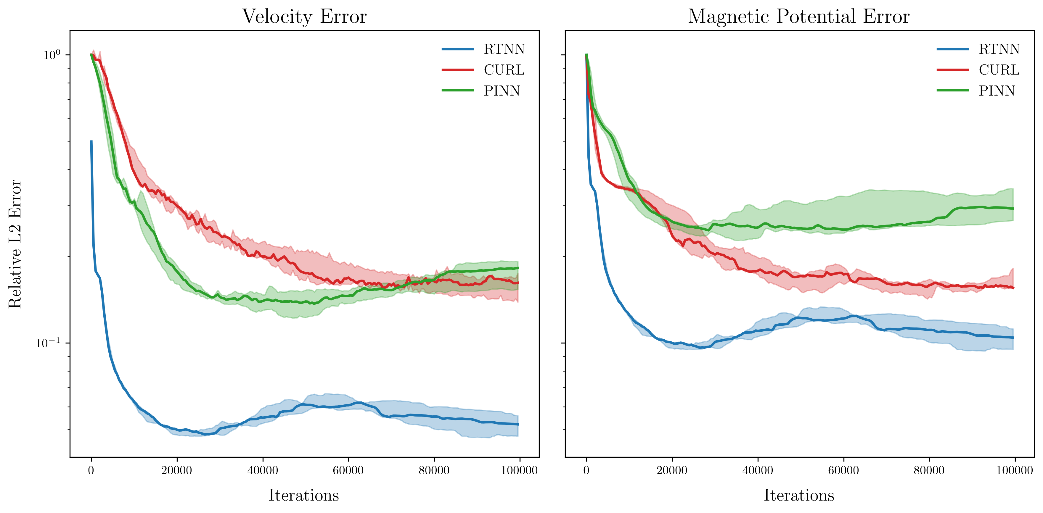
We train and validate our method on a three-dimensional periodic incompressible MHD flow in with Reynolds numbers and . The simulation covers the time interval for training and tests at . Training data is generated using a spectral solver, with initial velocity and magnetic field sampled from Gaussian random fields. Periodic boundary conditions are strictly enforced in all cases using the approach described in (Dong & Ni, 2021). We employ a Separable Physics-Informed Neural Network (SPINN) (Cho et al., 2023) comprising 5 hidden layers and 500 neurons per layer to handle the structured 3D grid, discretized into 101 × 128 × 128 points. The model is trained using 50,000 iterations of the L-BFGS optimizer. Validation at utilizes spectral solver data to evaluate performance. We compare three approaches: (i) our RTNN-based method, (ii) a SPINN baseline with penalized residuals, and (iii) a Curl-SPINN parametrizing velocity and magnetic fields as the curl of a scalar potential. Additional details and performance plots are provided in Section B.5.
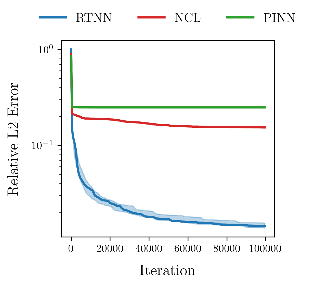
Results and Discussion
| Method | rL2 Error (Velocity) | rL2 Error (B) | Wall Time (s) |
|---|---|---|---|
| RTNN | 2.34e-02 | 1.04e-01 | 2340.41 |
| Curl-SPINN | 1.61e-01 | 1.55e-01 | 1191.67 |
| SPINN | 1.82e-01 | 2.93e-01 | 414.73 |
Table 3 reports the relative errors for both velocity and magnetic fields and Figure 5 shows the error evolution through training accross seeds. Our RTNN significantly improves velocity accuracy compared to the baselines and also enhances the accuracy of magnetic field predictions. Additionally, we demonstrated that RTNN can be incorporated into coupled systems for more complex problems.
4 Discussion and Conclusion
We introduced Riemann Tensor Neural Networks (RTNNs), a new class of neural architectures tailored for encoding divergence-free symmetric tensors (DFSTs). By construction, RTNNs exactly satisfy the DSFT conditions that encodes conservation of mass and momentum. Our theoretical results confirm that RTNNs are universal approximators of DFSTs, and our numerical benchmarks illustrate that they consistently improve accuracy compared to baselines such as standard PINNs and methods enforcing only part of the conservation (e.g., mass alone).
Limitations and Future Work
While our experiments focus on fluid dynamics applications using MLPs, RTNNs have the potential to extend to diverse systems like Euler–Fourier, relativistic Euler, Boltzmann, to name but a few. Future work includes enhancing algorithm performance, extending RTNNs to operator learning frameworks, and reducing computational costs by developing architectures with more efficient differential operators. Additionally, exploring function space optimization techniques (Jnini et al., 2024b; Müller & Zeinhofer, 2023) could further improve the accuracy of RTNNs.
Acknowledgments
A.J. acknowledges support from a fellowship provided by Leonardo S.p.A. L.B was funded by the European Union under NextGenerationEU. Views and opinions expressed are however those of the author(s) only and do not necessarily reflect those of the European Union or The European Research Executive Agency. Neither the European Union nor the granting authority can be held responsible for them.
5 Impact Statement
This paper presents work whose goal is to advance the field of Machine Learning. There are many potential societal consequences of our work, none which we feel must be specifically highlighted here.
References
- Bonfanti et al. (2024) Bonfanti, A., Bruno, G., and Cipriani, C. The challenges of the nonlinear regime for physics-informed neural networks. In The Thirty-eighth Annual Conference on Neural Information Processing Systems, 2024. URL https://openreview.net/forum?id=FY6vPtITtE.
- Bradbury et al. (2018) Bradbury, J., Frostig, R., Hawkins, P., Johnson, M. J., Leary, C., Maclaurin, D., Necula, G., Paszke, A., VanderPlas, J., Wanderman-Milne, S., and Zhang, Q. JAX: composable transformations of Python+NumPy programs, 2018. URL http://github.com/google/jax.
- Cai et al. (2021) Cai, S., Mao, Z., Wang, Z., Yin, M., and Karniadakis, G. E. Physics-informed neural networks (PINNs) for fluid mechanics: A review. Acta Mechanica Sinica, 37(12):1727–1738, 2021.
- Cho et al. (2023) Cho, J., Nam, S., Yang, H., Yun, S.-B., Hong, Y., and Park, E. Separable physics-informed neural networks, 2023. URL https://arxiv.org/abs/2306.15969.
- Dong & Ni (2021) Dong, S. and Ni, N. A method for representing periodic functions and enforcing exactly periodic boundary conditions with deep neural networks. Journal of Computational Physics, 435:110242, June 2021. ISSN 0021-9991. doi: 10.1016/j.jcp.2021.110242. URL http://dx.doi.org/10.1016/j.jcp.2021.110242.
- Ethier & Steinman (1994) Ethier, C. R. and Steinman, D. A. Exact fully 3d navier–stokes solutions for benchmarking. International Journal for Numerical Methods in Fluids, 19:369–375, 1994. URL https://api.semanticscholar.org/CorpusID:62789476.
- Giles & Maxwell (1987) Giles, C. L. and Maxwell, T. Learning, invariance, and generalization in high-order neural networks. Applied optics, 26(23):4972–4978, 1987.
- Greydanus et al. (2019a) Greydanus, S., Dzamba, M., and Yosinski, J. Hamiltonian neural networks. Advances in Neural Information Processing Systems, 32, 2019a.
- Greydanus et al. (2019b) Greydanus, S., Dzamba, M., and Yosinski, J. Hamiltonian neural networks, 2019b. URL https://arxiv.org/abs/1906.01563.
- Haghighat et al. (2021) Haghighat, E., Raissi, M., Moure, A., Gomez, H., and Juanes, R. A physics-informed deep learning framework for inversion and surrogate modeling in solid mechanics. Computer Methods in Applied Mechanics and Engineering, 379:113741, 2021.
- Hendriks et al. (2020) Hendriks, J., Jidling, C., Wills, A., and Schön, T. Linearly constrained neural networks. arXiv preprint arXiv:2002.01600, 2020.
- Hu et al. (2023) Hu, Z., Shukla, K., Karniadakis, G. E., and Kawaguchi, K. Tackling the curse of dimensionality with physics-informed neural networks. arXiv preprint arXiv:2307.12306, 2023.
- Jnini et al. (2024a) Jnini, A., Goordoyal, H., Dave, S., Korobenko, A., Vella, F., and Fraser, K. Physics-constrained deepONet for surrogate CFD models: a curved backward-facing step case. In ICLR 2024 Workshop on AI4DifferentialEquations In Science, 2024a. URL https://openreview.net/forum?id=zRef200Ucc.
- Jnini et al. (2024b) Jnini, A., Vella, F., and Zeinhofer, M. Gauss-newton natural gradient descent for physics-informed computational fluid dynamics. 2024b. URL https://api.semanticscholar.org/CorpusID:267740226.
- Karniadakis et al. (2021) Karniadakis, G. E., Kevrekidis, I. G., Lu, L., Perdikaris, P., Wang, S., and Yang, L. Physics-informed machine learning. Nature Reviews Physics, 3(6):422–440, 2021.
- Kidger & Lyons (2020) Kidger, P. and Lyons, T. Universal approximation with deep narrow networks, 2020. URL https://arxiv.org/abs/1905.08539.
- Kovachki et al. (2021) Kovachki, N., Li, Z., Liu, B., Azizzadenesheli, K., Bhattacharya, K., Stuart, A., and Anandkumar, A. Neural operator: Learning maps between function spaces. arXiv preprint arXiv:2108.08481, 2021.
- Lagaris et al. (1998) Lagaris, I. E., Likas, A., and Fotiadis, D. I. Artificial neural networks for solving ordinary and partial differential equations. IEEE transactions on neural networks, 9(5):987–1000, 1998.
- LeCun et al. (1998) LeCun, Y., Bottou, L., Bengio, Y., and Haffner, P. Gradient-based learning applied to document recognition. Proceedings of the IEEE, 86(11):2278–2324, 1998.
- Li et al. (2020) Li, Z., Kovachki, N., Azizzadenesheli, K., Liu, B., Bhattacharya, K., Stuart, A., and Anandkumar, A. Fourier neural operator for parametric partial differential equations. arXiv preprint arXiv:2010.08895, 2020.
- Müller & Zeinhofer (2023) Müller, J. and Zeinhofer, M. Achieving high accuracy with PINNs via energy natural gradient descent. ICML, 2023.
- Müller & Zeinhofer (2024) Müller, J. and Zeinhofer, M. Position: Optimization in sciml should employ the function space geometry, 2024. URL https://arxiv.org/abs/2402.07318.
- Nocedal & Wright (1999) Nocedal, J. and Wright, S. J. Numerical optimization. Springer, 1999.
- Raissi et al. (2019a) Raissi, M., Perdikaris, P., and Karniadakis, G. E. Physics-informed neural networks: A deep learning framework for solving forward and inverse problems involving nonlinear partial differential equations. Journal of Computational physics, 378:686–707, 2019a.
- Raissi et al. (2019b) Raissi, M., Perdikaris, P., and Karniadakis, G. E. Physics-informed neural networks: A deep learning framework for solving forward and inverse problems involving nonlinear partial differential equations. Journal of Computational physics, 378:686–707, 2019b.
- Richter-Powell et al. (2022) Richter-Powell, J., Lipman, Y., and Chen, R. T. Neural conservation laws: A divergence-free perspective. Advances in Neural Information Processing Systems, 35:38075–38088, 2022.
- Serre (1997) Serre, D. Solutions classiques globales des équations d’euler pour un fluide parfait incompressible. Annales de l’Institut Fourier, 47(1):139–153, 1997. URL https://www.numdam.org/articles/10.5802/aif.1563/.
- Serre (2018) Serre, D. Divergence-free positive symmetric tensors and fluid dynamics. Annales de l’Institut Henri Poincaré (Analyse Non Linéaire), 35(5):1209–1234, 2018. URL https://arxiv.org/abs/1705.00331.
- Serre (2019) Serre, D. Compensated integrability. applications to the vlasov–poisson equation and other models of mathematical physics. Journal de Mathématiques Pures et Appliquées, 127:67–88, 2019.
- Serre (2021) Serre, D. Hard spheres dynamics: Weak vs strong collisions. Archive for Rational Mechanics and Analysis, 240(1):243–264, 2021.
- Wang et al. (2021) Wang, S., Teng, Y., and Perdikaris, P. Understanding and mitigating gradient flow pathologies in physics-informed neural networks. SIAM Journal on Scientific Computing, 43(5):A3055–A3081, 2021.
Appendix A Proofs
A.1 Proof of Theorem 2.1
In this section, we prove the main result on the representation of divergence-free symmetric tensors (Theorem A.1), which states that (symmetric and divergence-free) exactly coincides with the image of the map , where satisfies Riemann-like symmetries.
We first recall the classification of Riemann-like -tensors (Lemma A.2), and then prove the surjectivity of the map (Lemma A.4). Combining these two ingredients completes the proof of Theorem A.1.
A.1.1 Main Theorem: Representation of Divergence-Free Symmetric Tensors
Theorem A.1 (Representation of Divergence-Free Symmetric Tensors on a Flat Manifold).
Let be an -dimensional real vector space with a fixed basis , and let denote the corresponding dual basis of . Let denote the space of 2-forms on . Consider the space of all -tensors defined on a flat manifold equipped with a Levi-Civita connection , satisfying the following symmetries:
-
1.
Antisymmetry within index pairs:
-
2.
Symmetry between pairs:
Let be a fixed basis of , where . Define the tensors:
Then:
-
1.
The space of divergence-free, symmetric -tensors on the flat manifold is exactly the image of the map
-
2.
Moreover, any such can be expressed as
where are smooth scalar functions.
Proof Outline.
By Lemma A.2, every with the above symmetries can be expanded in the basis . Hence can be written in the claimed form. We also check that is symmetric and divergence-free using flatness (commuting covariant derivatives) plus the antisymmetries. Finally, Lemma A.4 shows that any symmetric, divergence-free arises from some , establishing that the image of the map is the space of such .
A.1.2 Classification of Riemann-like Tensors
Lemma A.2 (Classification of Riemann-like -Tensors).
Let be an -dimensional real vector space, and let be the space of 2-forms on . Denote
Consider the vector space
There is a canonical vector-space isomorphism between this space and . In particular, its dimension is
Moreover, if is a basis for , then a corresponding basis in the space of such -tensors is given by
Proof of Lemma A.2.
Step 1: From to a symmetric bilinear form. Given with the stated symmetries, define for :
Since and are antisymmetric in their respective index pairs, and is antisymmetric in and , this is well-defined. The symmetry implies that is symmetric as a bilinear form on . Hence .
Step 2: From a symmetric bilinear form back to . Conversely, given , define
A straightforward check shows that inherits antisymmetry in , antisymmetry in , and the pair-exchange symmetry .
Step 3: Isomorphism and basis. These two constructions are linear inverses of each other, yielding a vector-space isomorphism between our -tensors and . The dimension follows from standard linear algebra. If is a basis of , then forms a basis for . Mapping these to -tensors via the above correspondence yields the stated basis . ∎
A.1.3 Surjectivity of the Map
As discussed, the second key ingredient for Theorem A.1 is showing that every divergence-free, symmetric -tensor can be obtained from some Riemann-like -tensor . Equivalently, the map
is surjective.
Lemma A.3 (Surjectivity of ).
Let be any Riemann-like -tensor (i.e. satisfying the symmetries of Lemma A.2). Define Then is automatically symmetric and divergence-free. Moreover, is onto: for any given symmetric, divergence-free -tensor , there exists a Riemann-like such that .
Proof.
Part 1: We first verify that if , then is symmetric and divergence-free.
- Symmetry: Using , we get
- Divergence-free: In flat space, covariant derivatives commute, so
Because is antisymmetric in , one shows that . Hence
Part 2 (Surjectivity): We now show that given any symmetric, divergence-free , we can solve for some Riemann-like . The argument below is spelled out for Dirichlet boundary conditions, but a similar idea works for Neumann or other boundary conditions.
A.2 Surjectivity of the map
Theorem A.4 (Surjectivity of the ).
We will now prove that the following map is surjective:
| (22) | ||||
| (23) |
where is a Riemann-like tensor and is a symmetric divergence-free tensor.
Proof.
This is equivalent to showing that for any given there exists a such that .
We will show it for Dirichlet boundary conditions, the proof for Neumann boundary conditions is similar but more complicated.
Let be symmetric, divergence-free and vanishing at the boundary:
| (24) | ||||
| (25) | ||||
| (26) |
Let be the Green’s function for the Laplacian operator with Dirichlet boundary conditions:
| (27) | ||||
| (28) |
Note that Green’s function satisfies .
Define as the convolution of with the Green’s function of the Laplacian:
| (29) |
We verify that is symmetric and divergence-free.
Since is symmetric (), we write:
| (30) | ||||
The divergence of is:
| (31) |
Using the fact that , we rewrite:
| (32) |
Using the identity:
| (33) |
We have:
| (34) | ||||
Since is divergence-free (), the first term vanishes:
| (35) |
| (36) |
and so, finally:
| (37) |
We have now a tensor with the following properties:
| (38) | ||||
We can now easily define a tensor with the desired properties from . Just let:
| (39) | ||||
We now verify the Riemann-like properties of :
| (40) | ||||
| (41) | ||||
| (42) | ||||
| (43) | ||||
So, since we can build an inverse for every , the map is surjective.
∎
A.2.1 Combining the Lemmas to Prove Theorem A.1
Proof of Theorem A.1.
(1) Symmetry and divergence-free for . By Lemma A.4 (Part 1), the tensor is always symmetric and divergence-free if is Riemann-like.
(2) Surjectivity: Every symmetric, divergence-free arises from some . By Lemma A.4 (Part-2), the map is onto the space of such .
(3) Basis and explicit representation. From Lemma A.2, any Riemann-like can be expanded in the basis . Consequently,
for some scalar functions . This shows that every can indeed be written in the claimed form.
Hence all parts of the statement hold, and the proof is complete. ∎
A.3 Proof of theorem A.5
Theorem A.5 (Universal Approximation for RTNN).
Let be a compact domain, and let be any divergence-free symmetric tensor field on . For any , there exists a Riemann Tensor Neural Network with a fixed narrow width and arbitrary depth, such that
| (44) |
where denotes the Frobenius norm.
Proof.
To prove Theorem A.5, we proceed in two main steps:
-
1.
Surjectivity of the Map from to : By Theorem A.4, the map
(45) defined by
(46) is surjective. This implies that for any divergence-free symmetric tensor field , there exists a tensor with Riemann-like symmetries such that
(47) -
2.
Approximation of Tensor Using Neural Networks: Since is a linear combination of scalar functions, specifically
(48) where are fixed basis tensors and are scalar coefficient functions, we can approximate each using deep narrow neural networks.
By the Universal Approximation Theorem for deep narrow neural networks (Kidger & Lyons, 2020), for each scalar function and for any , there exists a neural network such that
(49) where is a constant dependent on the norms of the basis tensors and the chosen tensor norm .
Construct the approximated tensor as
(50) Applying the map to , we obtain the approximated tensor :
(51) Error Propagation:
The approximation error in each propagates linearly to . Specifically, we have
(52) where accounts for the bounds on the second-order partial derivatives over the compact domain , and the final equality holds by the choice of .
Therefore, by appropriately choosing the neural networks to approximate each scalar coefficient within , we ensure that the approximated tensor satisfies
(53)
∎
Appendix B Additional resources for Experiments
B.1 Euler Equation
The simulation of the 2D isentropic Euler vortex is based on analytical solutions, ensuring precise modeling of vortex dynamics. Below, we provide detailed initial and boundary conditions, as well as a summary of the experimental setup parameters and hyperparameters.
| Parameter | Value |
|---|---|
| Optimizers | BFGS |
| Architecture | 4-layer Multilayer Perceptron, width 50 |
| Activation Function | Tanh |
| Domain | |
| Time Interval | |
| Collocation Points (Interior) | 1,000 |
| Collocation Points (Boundary) | 200 |
| Validation Points | 10,000 |
| Evaluation Metric | Relative Error |
Initial Conditions: The initial density, velocity components, and temperature distributions are defined based on the analytical solution of the Euler vortex:
| (54) | ||||
| (55) | ||||
| (56) | ||||
| (57) |
where represents the radial distance from the vortex center .
Boundary Conditions: On the boundaries of the spatial domain , we impose fixed values for density, velocity, and pressure:
B.2 Beltrami Flow
| Parameter | Value |
|---|---|
| Optimizers | BFGS |
| Architecture | 4-layer Multilayer Perceptron, width 50 |
| Activation Function | Tanh |
| Domain | |
| Time Interval | |
| Collocation Points (Interior) | 10,000 |
| Collocation Points (Boundary) | 961 per face |
| Validation Points | 10,000 |
| Evaluation Metric | Relative Error |
We consider the unsteady three-dimensional Beltrami flow originally described by Ethier & Steinman (1994) at . The spatial domain is and time ranges over . The exact solutions are:
and
These expressions satisfy the incompressible Navier–Stokes equations exactly, making the Beltrami flow an ideal test for verifying numerical methods. We use 10,000 interior collocation points to enforce the PDE residual and 961 boundary/initial points per face for constraints; an additional 10,000 points in the interior serve as a validation set. We report the training dynamics in Figure B.2.
B.3 Cylinder Wake
| Parameter | Value |
|---|---|
| Optimizers | BFGS |
| Architecture | 4-layer Multilayer Perceptron, width 50 |
| Activation Function | Tanh |
| Domain | |
| Time Interval | , |
| Interior Collocation Points | 40,000 |
| Boundary/Initial Points | 5,000 |
| Evaluation Metric | Relative Error |
For the two-dimensional cylinder wake at , we consider a circular cylinder centered at . The downstream domain is in space, with the simulation time interval discretized in increments of . We train a 4-layer MLP (width 50, Tanh activations) on 40,000 interior collocation points and 5,000 boundary/initial points, without using labeled data. We validate the solution against direct numerical simulation (DNS) from Raissi et al. (2019a). We report the training dynamics in Figure 3
B.4 NACA Airfoil
| Parameter | Value |
|---|---|
| Optimizers | BFGS |
| Architecture | 4-layer Multilayer Perceptron, width 50 |
| Activation Function | Tanh |
| Evaluation Metric | Relative Error |
We investigate the steady laminar flow at around a NACA 0012 airfoil. This problem is recast as a steady Navier–Stokes system by treating time as a dummy dimension. An MLP with 4 hidden layers (width 50, Tanh activations) is trained with labeled data from our in-house RANS solver with 2’000 data points and 40’000 collocation points for PDE residuals. We use 12’000 data points to validate the recovered fields. We report the training dynamics in Figure 4
B.5 MHD
We train and validate our method on a three-dimensional periodic incompressible Magnetohydrodynamics (MHD) flow within the domain , with Reynolds numbers and . The simulation covers the time interval for training and tests at . Training data is generated using a spectral solver, ensuring high accuracy, with initial velocity and magnetic field sampled from Gaussian random fields. Periodic boundary conditions are strictly enforced to maintain physical consistency across the domain. We employ a Separable Physics-Informed Neural Network (SPINN) (Cho et al., 2023) with 5 hidden layers and 500 neurons per layer to handle the structured 3D grid, discretized into 101 × 128 × 128 points along each respective dimension. The model is trained using 50,000 iterations of the L-BFGS optimizer to effectively minimize the loss function. Validation at utilizes spectral solver data to assess performance and ensure accurate replication of MHD flow characteristics. We compare three approaches: (i) our RTNN-based method, (ii) a SPINN baseline with penalized residuals, and (iii) a Curl-SPINN parametrizing velocity and magnetic fields as the curl of a scalar potential. Additional details and performance plots are provided below.
| Parameter | Value |
|---|---|
| Optimizer | L-BFGS |
| Architecture | Separable Physics-Informed Neural Network (SPINN) |
| Hidden Layers | 5 |
| Neurons per Layer | 500 |
| Activation Function | Tanh |
| Domain | |
| Time Interval | Training: , Testing: |
| Grid Discretization | points |
| Reynolds Number | |
| Magnetic Reynolds Number | |
| Training Iterations | 50,000 |
| Validation Data | Spectral solver data at |
| Evaluation Metric | Relative Error |
∎