Geodesic Diffusion Models for Medical Image-to-Image Generation

Abstract

Diffusion models transform an unknown data distribution into a Gaussian prior by progressively adding noise until the data become indistinguishable from pure noise. This stochastic process traces a path in probability space, evolving from the original data distribution (considered as a Gaussian with near-zero variance) to an isotropic Gaussian. The denoiser then learns to reverse this process, generating high-quality samples from random Gaussian noise. However, standard diffusion models, such as the Denoising Diffusion Probabilistic Model (DDPM), do not ensure a geodesic (i.e., shortest) path in probability space. This inefficiency necessitates the use of many intermediate time steps, leading to high computational costs in training and sampling. To address this limitation, we propose the Geodesic Diffusion Model (GDM), which defines a geodesic path under the Fisher-Rao metric with a variance-exploding noise scheduler. This formulation transforms the data distribution into a Gaussian prior with minimal energy, significantly improving the efficiency of diffusion models. We trained GDM by continuously sampling time steps from 0 to 1 and using as few as 15 evenly spaced time steps for model sampling. We evaluated GDM on two medical image-to-image generation tasks: CT image denoising and MRI image super-resolution. Experimental results show that GDM achieved state-of-the-art performance while reducing training time by 50× compared to DDPM and 10× compared to Fast-DDPM, with 66× faster sampling than DDPM and a similar sampling speed to Fast-DDPM. These efficiency gains enable rapid model exploration and real-time clinical applications. Our code is publicly available at: https://github.com/mirthAI/GDM-VE.

1 Introduction

Diffusion models [4, 8, 20, 21] have recently emerged as powerful tools for high-quality image generation [2, 17]. In the forward diffusion process, image data gradually transform into Gaussian noise, while the reverse diffusion process incrementally refines random noise into a high-quality image. Due to their ability to generate high-quality images with stable training, diffusion models have gained traction in medical imaging [16, 5, 15, 24]. However, achieving high-quality results typically requires hundreds to thousands of intermediate steps, posing a significant computational bottleneck, particularly for real-time medical applications.

Various methods have been proposed to accelerate the reverse sampling process. Training-based methods leverage knowledge distillation to train a smaller student model [18, 11, 13] or optimize the sampling trajectory for specific tasks [19, 14, 9]. However, these methods introduce additional computational overhead. Alternatively, efficient numerical solvers have been developed to efficiently solve the reverse stochastic or ordinary differential equation [20, 10]. More recently, Fast-DDPM [7] has been introduced to improve both training and sampling efficiency by optimizing time-step utilization.

We argue that standard diffusion models are suboptimal from a geometric perspective. The forward diffusion process traces a trajectory in the space of Gaussian distributions, starting with a Gaussian whose mean represents the image data and whose variance approaches zero, and ending with a prior Gaussian (e.g., a standard Gaussian). Ideally, this trajectory should be a geodesic—the shortest path under a Riemannian metric in probability space. A natural choice for this metric is the Fisher-Rao metric, which governs the curvature of how distributions evolve. However, existing diffusion models [4, 7] do not follow geodesic paths, causing the image distribution to traverse unnecessary or anomalous intermediate states. This inefficiency leads to suboptimal information propagation, longer training and sampling times, and degraded image quality. Enforcing a "straight-line" path in probability space could mitigate these issues, reducing computational costs while preserving generative quality.

We introduce the Geodesic Diffusion Model (GDM), which enforces a geodesic path between the image distribution and a prior Gaussian under the Fisher-Rao metric. This ensures optimal diffusion along the shortest path in both forward and reverse processes. With a geodesic noise scheduler, GDM transforms pure noise into the target distribution with minimal energy, accelerating model convergence during training. Since the diffusion path is a "straight line", fewer time steps are needed to solve the underlying differential equation, significantly improving sampling efficiency. We evaluated GDM on two conditional medical image-to-image generation tasks: CT image denoising using a single conditional image and MRI image super-resolution using two conditional images. GDM outperformed convolutional neural networks (CNNs), generative adversarial networks (GANs), DDPM [4], and Fast-DDPM [7] while also reducing training time by approximately 50× compared to DDPM and 10× compared to Fast-DDPM.

2 Methods

2.1 Mathematical Background

The forward diffusion process progressively adds noise to a high-quality image sample $x_{0}$ until it becomes indistinguishable from pure noise:

$$q(x_{t}|x_{0})=\mathcal{N}(x_{t};\alpha_{t}x_{0},\sigma_{t}^{2}\mathbb{I}),\quad t\in[0,1],$$ (1)

where $\alpha_{t}$ and $\sigma_{t}$ are continuous functions of time $t$. These functions are often referred to as the noise scheduler of the diffusion process. The two most common choices for noise schedulers are variance-preserving (VP) and variance-exploding (VE). In the VP setting, $\alpha_{t}$ monotonically decreases from $1$ to $0$, while $\sigma_{t}$ monotonically increases from $0$ to $1$. In the VE setting, $\alpha_{t}=1$ for all $t$, and $\sigma_{t}$ increases from $\sigma_{\min}$ to $\sigma_{\max}$, where $\sigma_{\min}$ is close to 0 and $\sigma_{\max}$ is much larger than 1.

With negligible error, we can approximate $x_{0}$ as a Gaussian distribution $\mathcal{N}(x_{0},\sigma_{\min}^{2}\mathbb{I})$ with near-zero variance. Under this assumption, Equation (1) defines a path in the space of Gaussian distributions with isotropic covariance. The widely DDPM and its variants employ a VP noise scheduler. However, this choice does not define a geodesic (i.e., the shortest) path in the space of Gaussian distributions, which can limit the efficiency of both model training and sampling. In this paper, we adopt the VE noise scheduler for mathematical simplicity in finding geodesics between the data distribution and a Gaussian prior. Under the VE setting, the diffusion process simplifies to:

$$q(x_{t}|x_{0})=\mathcal{N}(x_{0},\sigma_{t}^{2}\mathbb{I}),\quad t\in[0,1],$$ (2)

which can be expressed using the following stochastic differential equation (SDE):

$$dx_{t}=\sqrt{(\sigma_{t}^{2})^{\prime}}dW_{t},$$ (3)

where $W_{t}$ is a standard Wiener process. According to [21], the reverse process of $x_{t}$ can be described using an ordinary differential equation (ODE):

$$dx_{t}=-\frac{1}{2}(\sigma_{t}^{2})^{\prime}\nabla_{x_{t}}\log p(x_{t})\,dt,$$ (4)

where $p(x_{t})$ denotes the probability density of $x_{t}$. In diffusion models, we use neural networks to learn the score function $\nabla_{x_{t}}\log p(x_{t})$ for every given $x_{t}$, which enables us to solve the above ODE and generate new images from random noise.

2.2 The Fisher-Rao Metric

The Fisher-Rao metric is a natural Riemannian metric that determines the length of any path in the space of parameterized Gaussian distributions, enabling the identification of the shortest path between two Gaussian distributions. Given a probability distribution $p(x;\theta_{1},\dots,\theta_{k})$ parameterized by $\theta=(\theta_{1},\dots,\theta_{k})^{T}$, the Fisher information matrix $I(\theta)$ is defined as:

$$I(\theta)=\mathbb{E}\left[\frac{\partial\log p(x;\theta)}{\partial\theta}\left(\frac{\partial\log p(x;\theta)}{\partial\theta}\right)^{T}\right],$$ (5)

It quantifies the sensitivity of the probability distribution to variations in its parameters by capturing the expected curvature (second derivative) of the log-likelihood function. The Fisher information matrix defines the Riemannian metric in the space of probability distributions, and the Fisher-Rao distance is the geodesic distance induced by this metric:

$$d_{FR}(p(x;\theta_{1}),p(x;\theta_{2})=\min_{\theta(t)}\int_{0}^{1}\left|\dot{\theta}(t)\right|_{I(\theta(t))}dt,$$ (6)

where $\left|\dot{\theta}(t)\right|_{I(\theta(t))}=\sqrt{\dot{\theta}(t)^{T}I(\theta(t))\dot{\theta}(t)}$ and $p(x;\theta(t))$ is a path connecting the two distributions $p(x;\theta_{1})$ and $p(x;\theta_{2})$.

2.3 Geodesic Diffusion Models

Consider a multivariate Gaussian distribution with an isotropic covariance matrix: $p(x|\mu,\sigma)=\frac{1}{(2\pi\sigma^{2})^{n/2}}\exp\left(-\frac{1}{2\sigma^{2}}\|x-\mu\|^{2}\right)$, where the parameter vector is given by $\theta=(\mu,\sigma)^{T}$. The corresponding Fisher information matrix is given by:

$$I(\theta)=\begin{bmatrix}\frac{1}{\sigma^{2}}I&0\\ 0&\frac{2n}{\sigma^{2}}\end{bmatrix}.$$ (7)

To simplify our analysis, we focus on variance-exploding noise schedulers, where the latent variable follows: $x_{t}\sim\mathcal{N}(x_{t};x_{0},\sigma^{2}_{t}\mathbb{I})$, with $\theta=\sigma$. The length of a path connecting two distributions $\mathcal{N}(x_{0},\sigma_{\min}^{2}\mathbb{I})$ and $\mathcal{N}(x_{0},\sigma_{\max}^{2}\mathbb{I})$ is:

$$L=\int_{0}^{1}\sqrt{\frac{2n(\dot{\sigma}_{t})^{2}}{\sigma_{t}^{2}}}dt=\int_{0}^{1}\sqrt{2n}\frac{\dot{\sigma}_{t}}{\sigma_{t}}dt=\sqrt{2n}\cdot\ln\left(\frac{\sigma_{\max}}{\sigma_{\min}}\right).$$ (8)

Since geodesic paths must maintain a constant speed, we have:

$$\sigma_{t}=\sigma_{\min}\left(\frac{\sigma_{\max}}{\sigma_{\min}}\right)^{t}.$$ (9)

Here, we propose Geodesic Diffusion Models (GDMs), which use the noise scheduler from Equation 9. Unlike DDPM, which follows a non-optimal path, GDM traverses the shortest path in probability space and therefore (1) converges faster during training, (2) requires fewer diffusion steps during sampling, and (3) reduces computational cost while maintaining high-quality image generation.

2.3.1 Model Training

We apply the geodesic diffusion model to conditional image-to-image generation tasks, where the goal is to generate a high-quality image $x_{0}$ given a conditional image $c$. We denote the joint distribution of the image and its conditional counterpart as $p_{\text{joint}}(x_{0},c)$, and the marginal distribution of conditional images as $p_{c}(c)$.

During training, we randomly sample pairs $(x_{0},c)\sim p_{\text{joint}}(x_{0},c)$ and time steps $t\sim U([0,1])$. We then perturb $x_{0}$ by adding noise: $x_{t}=x_{0}+\sigma_{t}\epsilon$, where $\epsilon\sim\mathcal{N}(0,\mathbb{I})$ is a random noise sample, and $\sigma_{t}$ is defined in Equation 9. We train a U-Net denoiser using the following loss function:

$$E_{(x_{0},c),t,\epsilon}\left\|\epsilon-\epsilon_{\theta}\big{(}x_{0}+\sigma_{t}\epsilon,c,t\big{)}\right\|^{2}.$$ (10)

where $\epsilon_{\theta}$ estimates the score function (up to a scaling factor) at each $x_{t}$, i.e., it estimates $\epsilon=-\sigma_{t}\nabla_{x_{t}}\log p(x_{t})$.

2.3.2 Model Sampling

During model sampling, we use $N$ uniformly spaced time steps between $t=1$ and $t=0$. In our experiments, we set $N=15$. The sampling process begins by drawing random noise $x_{1}$ from the prior Gaussian distribution $\mathcal{N}(0,\sigma_{\max}^{2}\mathbb{I})$ and conditioning on an image $c$. We then employ a first-order Euler solver to approximate the solution to the reverse ODE (Equation 4), given by:

$$x_{t_{k-1}}=x_{t_{k}}+(t_{k-1}-t_{k})\dot{\sigma}_{t_{k}}\epsilon_{\theta}(x_{t_{k}},c,t_{k})$$ (11)

where $t_{k}$ and $t_{k-1}$ denote the current and next time steps in the denoising process, $\dot{\sigma}_{t_{k}}$ represents the time derivative of the geodesic variance-exploding noise schedule at $t_{k}$, and $\epsilon_{\theta}$ is the trained image denoiser. The complete sampling procedure is outlined in Algorithm 1.

1 Hyperparameter: number of sampling steps $N$

2 $x_{1}\sim\mathcal{N}(0,\sigma_{max}^{2}\mathbb{I})$

3 $c\sim p_{\text{c}}(c)$

4 for $k=N,\cdots,1$  do

5    $x_{t_{k-1}}=x_{t_{k}}+(t_{k-1}-t_{k})\dot{\sigma}_{t_{k}}\epsilon_{\theta}(x_{t_{k}},c,t_{k})$

6   

7 end for

return $x_{0}$

Algorithm 1 Sampling of Geodesic Diffusion Model

3 Experiments and Results

We evaluated our geodesic diffusion model on two conditional image generation tasks: CT image denoising, conditioned on a single low-dose CT image, and multi-image MRI super-resolution, conditioned on two neighboring MR slices.

3.1 Datasets and Implementation Details

3.1.1 Low-Dose and Full-Dose Lung CT Dataset

The publicly available dataset [12] includes paired low-dose and normal-dose chest CT volumes. Normal-dose scans were acquired at standard clinical dose levels, while low-dose scans were simulated at 10% of the routine dose. The dataset comprises 48 patients, with 38 randomly assigned for training and 10 for evaluation, resulting in 13,211 and 3,501 pairs of 2D low-dose and normal-dose CT images, respectively. All images were resized to 256 × 256 pixels and normalized to the range [-1, 1].

3.1.2 Prostate MRI Dataset

The publicly available dataset [22] consists of MRI volumes with an in-plane resolution of 0.547 mm × 0.547 mm and an inter-slice distance of 1.5 mm. For training and testing, we formed triplets of three consecutive MRI slices, using the first and third slices as the input and the middle slice as the ground truth. In total, we extracted 6,979 triplets from 120 MRI volumes for training and 580 triplets from 10 MRI volumes for evaluation. All slices were resized to 256 × 256 pixels and normalized to the range [-1, 1].

3.1.3 Evaluation Metrics

To assess the quality of the generated images, we used Peak Signal-to-Noise Ratio (PSNR) and Structural Similarity Index Measure (SSIM). PSNR quantifies the difference between the generated and ground-truth images by measuring the ratio of maximum possible signal power to distortion, with higher values indicating better fidelity. SSIM evaluates perceived image quality by comparing luminance, contrast, and structural details, providing a more perceptually relevant assessment than PSNR.

3.1.4 Implementation Details

Our model is based on a U-Net architecture from DDIM [20]. We use the Adam optimizer with a learning rate of 0.0002 and a batch size of 16. The training is conducted using Python 3.10.6 and PyTorch 1.12.1. All experiments are performed on a single NVIDIA A100 GPU with 80GB of memory. In Equation 9, we set $\sigma_{\text{min}}=0.002$ and $\sigma_{\text{max}}=80$.

3.2 CT Image Denoising

Table 1 compares GDM’s performance and computational efficiency with four baseline models, including two diffusion models (DDPM and Fast-DDPM), a convolution-based model (REDCNN [1]), and a GAN-based method (DU-GAN [6]), for CT denoising. GDM significantly improves computational efficiency, reducing training time by 56.4× compared to DDPM and 10.4× compared to Fast-DDPM, due to its geodesic diffusion path. It also achieves the best image generation quality while maintaining an inference time comparable to Fast-DDPM and 68× shorter than DDPM. These results demonstrate GDM’s effectiveness in delivering high-quality denoising with improved efficiency.

Table 1: Quantitative results of CT image denoising. DDPM, Fast-DDPM, and GDM converged at 2 M, 400 K, and only 45 K iterations, respectively.

Model	PSNR	SSIM	Training Time	Inference Time
REDCNN [1]	36.37	0.910	3 h	0.5 s
DU-GAN [6]	36.25	0.902	20 h	3.8 s
DDPM [4]	35.36	0.873	141 h	21.4 min
Fast-DDPM [7]	37.47	0.916	26 h	12.5 s
GDM	37.88	0.924	2.5 h	18.8 s

Figure 1 presents a low-dose lung CT, its corresponding normal-dose CT, and the normal-dose predictions from each model. The lung fissure in the normal-dose CT was not successfully reconstructed by REDCNN and DU-GAN. In contrast, diffusion-based methods preserved the fissure structure, with GDM generating the clearest and most continuous reconstruction. This enables more precise lung partitioning and enhances disease analysis across regions separated by the fissure.

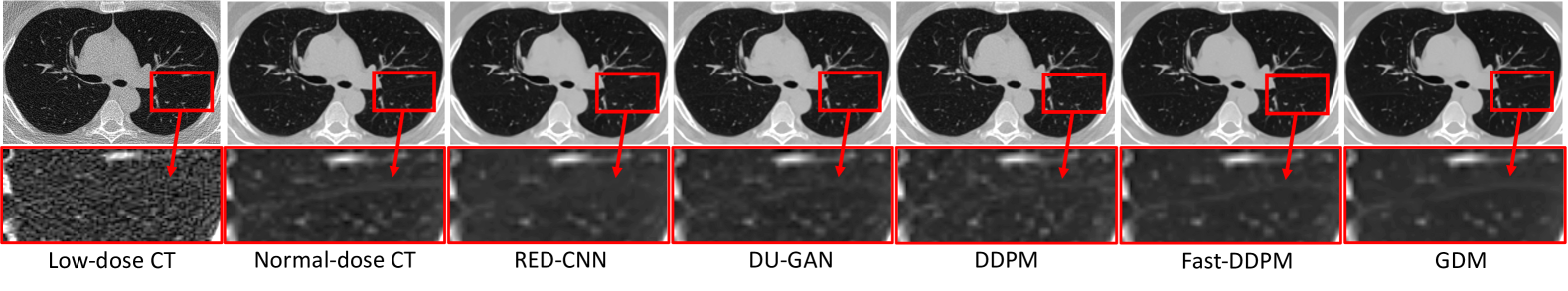
Figure 1: Qualitative results of CT image denoising.

3.3 MR Image Super-Resolution

Table 2 compares GDM with a convolution-based method (miSRCNN [3] ), a GAN-based method (miSRGAN [23]), and two diffusion models for MRI image super-resolution. The results show that GDM achieves state-of-the-art performance, attaining the highest PSNR (27.42) and SSIM (0.893) among all models. GDM also enhances computational efficiency, reducing training time to just 3 hours, compared to 136 hours for DDPM and 26 hours for Fast-DDPM. Moreover, while matching Fast-DDPM in inference speed, GDM further improves image quality, demonstrating its effectiveness in both efficiency and performance.

Table 2: Quantitative results of Super-Resolution: DDPM, Fast-DDPM, and GDM trained with 2M, 400k, and only 45k iterations, miSRCNN, miSRGAN

Model	PSNR	SSIM	Training Time	Inference Time
miSRCNN [3]	26.48	0.870	1 h	0.01 s
miSRGAN [23]	26.79	0.880	40 h	0.04 s
DDPM [4]	25.31	0.831	136 h	3.7 min
Fast-DDPM [7]	27.09	0.887	26 h	2.3 s
GDM	27.42	0.893	3 h	3.5 s

Figure 2 shows the results of predicting the center MRI slice from the previous and next slices in a prostate MRI triplet. The bright spots in the upper left corner of the center slice were not well predicted by DDPM, while our GDM model produced an image with intensity resembling the ground truth center slice and the clearest reconstruction.

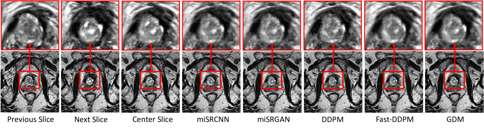
Figure 2: Qualitative results of MRI image super-resolution.

3.4 Ablation Study

Table 3 evaluates the impact of the number of sampling steps on the performance of GDM across the denoising and super-resolution tasks. The results indicate that GDM achieves its best generation performance with 15 sampling steps, reaching the highest PSNR and SSIM. Notably, increasing the number of sampling steps beyond 15 does not lead to an improvement in performance. This may be because GDM follows a geodesic path, and the noise scheduler already optimally guides the model, making extra steps unnecessary and inefficient.

Table 3: Performance of GDM with different numbers of sampling steps.

Sampling Steps	Denoising		Super Resolution
	PSNR	SSIM	PSNR	SSIM
15	37.88	0.924	27.42	0.893
20	37.87	0.923	27.39	0.893
100	37.30	0.910	27.39	0.892
1000	36.11	0.890	26.31	0.872

4 Discussion and Conclusion

This work introduces Geodesic Diffusion Models (GDMs), which optimize the diffusion process by ensuring that the transformation between data distributions follows the shortest path in probability space. This structured approach reduces inefficiencies, allowing for a more direct and computationally effective generative process. Experimental results demonstrate that GDM achieves competitive performance across various medical image generation tasks while significantly reducing computational overhead. These improvements highlight the potential of GDMs in advancing medical imaging research and real-time clinical applications.

Future work will explore extensions of GDM to three-dimensional medical image generation and further investigate adaptive noise schedulers that dynamically optimize the diffusion trajectory. Additionally, we aim to evaluate GDM’s applicability in multi-modal medical imaging to enhance integration across different data sources. The flexibility and efficiency of GDM make it a promising direction for future developments in diffusion-based generative modeling.

References

- [1] Hu Chen, Yi Zhang, Mannudeep K. Kalra, Feng Lin, Yang Chen, Peixi Liao, Jiliu Zhou, and Ge Wang. Low-dose ct with a residual encoder-decoder convolutional neural network. IEEE Transactions on Medical Imaging, 36(12):2524–2535, 2017.
- [2] Prafulla Dhariwal and Alexander Nichol. Diffusion models beat gans on image synthesis. Advances in neural information processing systems, 34:8780–8794, 2021.
- [3] Chao Dong, Chen Change Loy, Kaiming He, and Xiaoou Tang. Image super-resolution using deep convolutional networks. IEEE Transactions on Pattern Analysis and Machine Intelligence, 38(2):295–307, 2016.
- [4] Jonathan Ho, Ajay Jain, and Pieter Abbeel. Denoising diffusion probabilistic models. Advances in neural information processing systems, 33:6840–6851, 2020.
- [5] Xinrong Hu, Yu-Jen Chen, Tsung-Yi Ho, and Yiyu Shi. Conditional diffusion models for weakly supervised medical image segmentation, 2023.
- [6] Zhizhong Huang, Junping Zhang, Yi Zhang, and Hongming Shan. Du-gan: Generative adversarial networks with dual-domain u-net-based discriminators for low-dose ct denoising. IEEE Transactions on Instrumentation and Measurement, 71:1–12, 2022.
- [7] Hongxu Jiang, Muhammad Imran, Linhai Ma, Teng Zhang, Yuyin Zhou, Muxuan Liang, Kuang Gong, and Wei Shao. Fast-ddpm: Fast denoising diffusion probabilistic models for medical image-to-image generation. arXiv preprint arXiv:2405.14802, 2024.
- [8] Diederik P Kingma and Max Welling. Auto-encoding variational bayes. arXiv preprint arXiv:1312.6114, 2013.
- [9] Zhifeng Kong and Wei Ping. On fast sampling of diffusion probabilistic models, 2021.
- [10] Cheng Lu, Yuhao Zhou, Fan Bao, Jianfei Chen, Chongxuan Li, and Jun Zhu. Dpm-solver: A fast ode solver for diffusion probabilistic model sampling in around 10 steps. Advances in Neural Information Processing Systems, 35:5775–5787, 2022.
- [11] Eric Luhman and Troy Luhman. Knowledge distillation in iterative generative models for improved sampling speed. arXiv preprint arXiv:2101.02388, 2021.
- [12] C McCollough, B Chen, D Holmes, X Duan, Z Yu, L Xu, S Leng, and J Fletcher. Low dose ct image and projection data (ldct-and-projection-data)(version 4). Med. Phys, 48:902–911, 2021.
- [13] Chenlin Meng, Robin Rombach, Ruiqi Gao, Diederik Kingma, Stefano Ermon, Jonathan Ho, and Tim Salimans. On distillation of guided diffusion models. In Proceedings of the IEEE/CVF Conference on Computer Vision and Pattern Recognition, pages 14297–14306, 2023.
- [14] Alexander Quinn Nichol and Prafulla Dhariwal. Improved denoising diffusion probabilistic models. In International conference on machine learning, pages 8162–8171. PMLR, 2021.
- [15] Muzaffer Özbey, Onat Dalmaz, Salman UH Dar, Hasan A Bedel, Şaban Özturk, Alper Güngör, and Tolga Çukur. Unsupervised medical image translation with adversarial diffusion models. IEEE Transactions on Medical Imaging, 2023.
- [16] Walter HL Pinaya, Petru-Daniel Tudosiu, Jessica Dafflon, Pedro F Da Costa, Virginia Fernandez, Parashkev Nachev, Sebastien Ourselin, and M Jorge Cardoso. Brain imaging generation with latent diffusion models. In MICCAI Workshop on Deep Generative Models, pages 117–126. Springer, 2022.
- [17] Robin Rombach, Andreas Blattmann, Dominik Lorenz, Patrick Esser, and Björn Ommer. High-resolution image synthesis with latent diffusion models. In Proceedings of the IEEE/CVF conference on computer vision and pattern recognition, pages 10684–10695, 2022.
- [18] Tim Salimans and Jonathan Ho. Progressive distillation for fast sampling of diffusion models. arXiv preprint arXiv:2202.00512, 2022.
- [19] Robin San-Roman, Eliya Nachmani, and Lior Wolf. Noise estimation for generative diffusion models. arXiv preprint arXiv:2104.02600, 2021.
- [20] Jiaming Song, Chenlin Meng, and Stefano Ermon. Denoising diffusion implicit models. arXiv preprint arXiv:2010.02502, 2020.
- [21] Yang Song, Jascha Sohl-Dickstein, Diederik P Kingma, Abhishek Kumar, Stefano Ermon, and Ben Poole. Score-based generative modeling through stochastic differential equations. arXiv preprint arXiv:2011.13456, 2020.
- [22] Geoffrey A Sonn, Shyam Natarajan, Daniel JA Margolis, Malu MacAiran, Patricia Lieu, Jiaoti Huang, Frederick J Dorey, and Leonard S Marks. Targeted biopsy in the detection of prostate cancer using an office based magnetic resonance ultrasound fusion device. The Journal of urology, 189(1):86–92, 2013.
- [23] Rewa R. Sood, Wei Shao, Christian Kunder, Nikola C. Teslovich, Jeffrey B. Wang, Simon J.C. Soerensen, Nikhil Madhuripan, Anugayathri Jawahar, James D. Brooks, Pejman Ghanouni, Richard E. Fan, Geoffrey A. Sonn, and Mirabela Rusu. 3d registration of pre-surgical prostate mri and histopathology images via super-resolution volume reconstruction. Medical Image Analysis, 69:101957, 2021.
- [24] Boxiao Yu, Savas Ozdemir, Yafei Dong, Wei Shao, Tinsu Pan, Kuangyu Shi, and Kuang Gong. Robust whole-body pet image denoising using 3d diffusion models: evaluation across various scanners, tracers, and dose levels. European Journal of Nuclear Medicine and Molecular Imaging, pages 1–14, 2025.