Multi-Cali Anything: Dense Feature Multi-Frame Structure-from-Motion for Large-Scale Camera Array Calibration
Abstract
Calibrating large-scale camera arrays, such as those in dome-based setups, is time-intensive and typically requires dedicated captures of known patterns. While extrinsics in such arrays are fixed due to the physical setup, intrinsics often vary across sessions due to factors like lens adjustments or temperature changes. In this paper, we propose a dense-feature-driven multi-frame calibration method that refines intrinsics directly from scene data, eliminating the necessity for additional calibration captures. Our approach enhances traditional Structure-from-Motion (SfM) pipelines by introducing an extrinsics regularization term to progressively align estimated extrinsics with ground-truth values, a dense feature reprojection term to reduce keypoint errors by minimizing reprojection loss in the feature space, and an intrinsics variance term for joint optimization across multiple frames. Experiments on the Multiface dataset show that our method achieves nearly the same precision as dedicated calibration processes, and significantly enhances intrinsics and 3D reconstruction accuracy. Fully compatible with existing SfM pipelines, our method provides an efficient and practical plug-and-play solution for large-scale camera setups. Our code is publicly available at: https://github.com/YJJfish/Multi-Cali-Anything
I INTRODUCTION
Camera calibration is a crucial task in computer vision, particularly for applications like multi-view 3D reconstruction, virtual reality (VR), and augmented reality (AR). It involves estimating intrinsic parameters (e.g., focal lengths, principal points, and distortion coefficients) and extrinsic parameters (rotation and translation) that define the geometric relationship between the image and the world. Traditional methods use images of well-defined patterns, such as checkerboards, to achieve accurate parameter estimation.
While effective, these methods face limitations in large-scale systems, such as VR headsets or camera domes with dozens or hundreds of cameras. The primary challenge lies in the necessity for an additional calibration capture session before each scene capture. Although the extrinsics in these systems remain stable due to their physical setup, intrinsics often change due to factors like lens adjustments or temperature changes. Consequently, every time the intrinsics change, a new time-consuming calibration process is required before capturing actual scene data. The inefficiency of this workflow motivates the need for more efficient solutions.
Recent advances in Structure-from-Motion (SfM) pipelines, such as Pixel-Perfect SfM [1] and VGGSfM [2], have provided efficient tools for joint estimation of camera parameters and 3D scene structure. These methods can perform camera calibration directly from scene data without a separate calibration session. However, SfM pipelines are typically designed to estimate extrinsics and intrinsics simultaneously, and they do not provide an option to utilize known ground-truth extrinsics and refine only intrinsics, leading to suboptimal intrinsics calibration. In large-scale camera array setups where the extrinsics are already well-known, this lack of flexibility results in unnecessary estimation errors and reduced accuracy. Besides, the single frame processing of these pipelines causes inconsistencies in multi-frame datasets, reducing accuracy and robustness.
To overcome these challenges, we propose a dense-feature-driven multi-frame calibration method optimized for large-scale setups. By leveraging outputs from SfM pipelines and assuming stable extrinsics from a one-time calibration, our method refines intrinsic parameters and improves sparse 3D reconstructions without requiring dedicated calibration captures. This approach is ideal for scenarios where extrinsics are stable but intrinsics frequently change, achieving state-of-the-art results on the Multiface [3] dataset.
The primary contributions of our method are threefold:
-
•
We propose an extrinsics regularization method to iteratively refine estimated extrinsics toward ground-truth, ensuring robust convergence without local minima.
-
•
We introduce a dense feature reprojection term that minimizes reprojection errors in the feature space, reducing the influence of keypoint noise.
-
•
We design a multi-frame optimization method which uses an intrinsics variance term to get more accurate intrinsics across frames for multi-frame datasets.
This paper is organized as follows. Section II reviews prior work on camera calibration and SfM. Section III presents our proposed method in detail. Section IV conducts experiments on the Multiface dataset, including quantitative comparisons, qualitative results, and ablation study. Section V summarizes the contributions and outlines future work.
II RELATED WORK
Camera calibration and SfM have been extensively studied for reconstructing 3D scenes and estimating camera parameters. Here, we review prior work in three key areas: traditional calibration methods, general SfM techniques, and recent advances leveraging dense features, highlighting their limitations in the context of large-scale camera arrays with fixed extrinsics and varying intrinsics.
Traditional camera calibration typically relies on controlled setups with known patterns or objects. For instance, Loaiza et al. [4] proposed a one-dimensional invariant pattern with four collinear markers, leveraging its simplicity for multi-camera systems. Usamentiaga et al. [5] introduced a calibration plate with laser-illuminated protruding cylinders for precise 3D measurements, while Huang et al. [6] utilized a cubic chessboard to enforce multi-view constraints. These methods offer high accuracy but require dedicated calibration sessions, limiting scalability for large-scale arrays due to spatial constraints and setup overhead. To address scalability, Moreira et al. [7] proposed VICAN, an efficient algorithm for large camera networks that estimates extrinsics using dynamic objects and bipartite graph optimization. While effective for extrinsic calibration, VICAN does not refine intrinsics independently, a critical need in fixed setups where intrinsics vary across sessions due to lens adjustments or environmental factors.
SfM-based calibration methods provide a scalable alternative by jointly estimating camera parameters and 3D structures from scene data. COLMAP [8, 9] is a widely adopted pipeline, balancing robustness and efficiency through incremental optimization. OpenMVG [10] and HSfM [11] enhance scalability with modular designs and hierarchical processing, respectively. Pixel-Perfect SfM [1] improves precision by refining keypoints with featuremetric optimization, reducing reprojection errors. Recent global approaches, such as GLOMAP [12], revisit SfM with deep features for consistent multi-view registration. However, these methods typically estimate intrinsics and extrinsics simultaneously, lacking flexibility to refine intrinsics alone when extrinsics are fixed—a common scenario in dome-based camera arrays.
Deep learning has further advanced SfM. VGGSfM [2] introduces an end-to-end differentiable pipeline with visual geometry grounding, improving feature robustness, though it assumes centered principal points, reducing adaptability. DUSt3R [13] predicts dense point maps unsupervised, enhancing 3D reconstruction but sacrificing geometric precision in camera parameters. Feature extraction methods like SIFT [14], SuperPoint [15], R2D2 [16], and DISK [17], paired with matching techniques such as SuperGlue [18] and S2DNet [19], provide reliable correspondences, indirectly supporting SfM. Despite these advances, general SfM methods lack mechanisms for multi-frame consistency, crucial for refining intrinsics across sessions in fixed arrays.
Recent SfM research has shifted toward dense feature matching to improve robustness and reconstruction quality. Seibt et al. [20] introduced DFM4SFM, which leverages dense feature matching with homography decomposition to enhance correspondence accuracy in SfM, particularly for challenging scenes. Similarly, Lee and Yoo [21] proposed Dense-SfM, integrating dense consistent matching with Gaussian splatting to achieve dense, accurate 3D reconstructions, excelling in texture-sparse regions. Detector-Free SfM [22] eliminates traditional keypoint detectors, relying entirely on dense matching for robustness, though at a high computational cost. These methods demonstrate the power of dense features but are designed for general SfM tasks, optimizing both intrinsics and extrinsics without exploiting known extrinsics or ensuring multi-frame consistency.
Our approach is motivated to target large-scale camera arrays with fixed extrinsics. We build on existing SfM pipelines by introducing additional refinements with extrinsics regularization, dense-feature reprojection, and multi-frame optimization to refine intrinsics directly from scene data. Unlike traditional calibration methods, our method eliminates the necessity for dedicated calibration captures while still achieving high precision. Different from other SfM pipelines [8, 1, 2] which do not provide intrinsic-only refinement, our method utilizes known ground-truth extrinsics to improve the accuracy of intrinsics. Achieving nearly the same precision as dedicated calibration methods on the Multiface [3] dataset, our plug-and-play solution advances scalable calibration for real-world applications.
III APPROACH
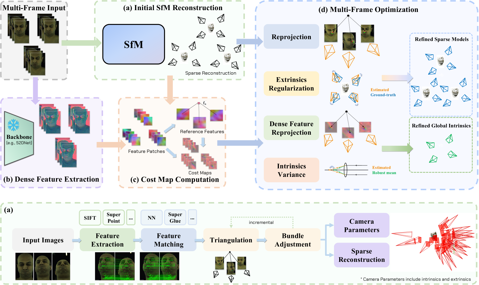
Fig. 1 illustrates the architecture of our proposed method: (a) shows the initial SfM process, which acts as the foundation of the pipeline. (b) highlights the dense feature extraction module, where a backbone network, such as S2DNet, is used to compute dense feature maps from the input images, capturing rich feature details. (c) focuses on cost map computation, a crucial step for optimizing memory and computational efficiency. Computing reprojection errors based on raw dense feature maps can be time-consuming and memory-intensive. Instead, these dense feature maps can be proprocessed into compact cost maps to significantly reduce resource usage and improve efficiency. Finally, (d) presents the optimization stage, which performs a multi-frame dense-feature-driven bundle adjustment (BA). This module refines both sparse reconstructions and camera parameters, outputting a globally consistent set of camera intrinsics and enhanced sparse reconstructions.
III-A Background
In this work, a frame refers to a specific time point at which multiple cameras simultaneously capture the object. Each camera captures one image per frame, resulting in a unique image for every combination of a frame and a camera. Formally, given a dataset with frames and cameras, the total number of captured images is . This assumption is valid under large-scale camera array in dome-based setups. Besides, we assume all cameras follow the pinhole camera model, with four intrinsic parameters: , , , . However, it is easy to be extended to more complex models.
Traditional BA minimizes the total reprojection loss:
| (1) |
where is the frame index. The subscript is needed because traditional BA only works with single frame data. is the set of triangulated 3D points in the -th frame. is a set of (camera index, 2D keypoint) pairs in the track of the 3D point . For example, means the 3D point is observed in the -th camera view, and its corresponding 2D keypoint in the image space is . , , are estimated extrinsics and intrinsics of the -th camera, based on the -th frame data. transforms and projects a point in the 3D world space to 2D image space. is a loss function (e.g. Cauchy loss). In this work, we use:
| (2) |
where represents the normalized reprojection loss, which is normalized by the total number of observations and incorporates a weighting factor to balance with other loss terms, ensuring robustness across frames with varying numbers of observations.
| Method | ‰ | ‰ | ‰ | ‰ | ‰ | ‰ | |||||||||
| COLMAP [8, 9] (SIFT [14]+NN) | 240.107 | 370.769 | 197.697 | 31.610 | 48.867 | 26.095 | 66.786 | 112.163 | 47.742 | 42.415 | 72.848 | 29.834 | |||
| Fix Extrinsic | 117.781 | 122.004 | 112.627 | 15.574 | 16.136 | 14.897 | 1.594 | 1.682 | 1.455 | 0.955 | 1.010 | 0.873 | |||
| Pixel-Perfect [1] (Disk [17]+NN) | 313.362 | 359.700 | 268.225 | 41.203 | 47.331 | 35.277 | 66.886 | 76.557 | 58.248 | 42.040 | 49.425 | 36.684 | |||
| Fix Extrinsic | 179.227 | 183.157 | 176.467 | 23.683 | 24.205 | 23.320 | 5.264 | 5.447 | 5.078 | 2.909 | 3.001 | 2.798 | |||
| Pixel-Perfect (R2D2 [16]+NN) | 126.477 | 211.908 | 64.953 | 16.540 | 27.800 | 8.501 | 61.212 | 96.716 | 42.744 | 39.093 | 63.352 | 26.318 | |||
| Fix Extrinsic | 91.132 | 103.760 | 83.591 | 12.052 | 13.727 | 11.054 | 2.950 | 3.358 | 2.603 | 1.860 | 2.043 | 1.647 | |||
| Pixel-Perfect (SuperPoint [15]+NN) | 406.536 | 728.230 | 138.871 | 53.937 | 97.041 | 18.185 | 220.455 | 469.903 | 107.160 | 137.272 | 279.020 | 66.045 | |||
| Fix Extrinsic | 10.456 | 24.965 | 4.414 | 1.389 | 3.313 | 0.582 | 2.686 | 4.290 | 1.883 | 1.726 | 2.521 | 1.257 | |||
| Pixel-Perfect (SuperPoint+SuperGlue [18]) | 490.563 | 634.495 | 227.274 | 65.008 | 84.246 | 30.119 | 207.518 | 300.653 | 142.050 | 130.619 | 190.479 | 86.182 | |||
| Fix Extrinsic | 7.307 | 14.157 | 3.808 | 0.965 | 1.873 | 0.502 | 2.391 | 3.534 | 1.384 | 1.563 | 2.146 | 0.986 | |||
| DUSt3R [13] (Linear) | 5854.966 | 5982.099 | 5570.567 | 774.200 | 791.681 | 739.994 | 163.994 | 164.348 | 163.778 | 104.706 | 104.928 | 104.567 | |||
| Fix Extrinsic | 5885.447 | 6087.489 | 5602.540 | 776.848 | 805.607 | 742.758 | 156.384 | 157.863 | 154.685 | 93.320 | 94.269 | 92.218 | |||
| DUSt3R (DPT) | 9959.293 | 10114.131 | 9760.731 | 1309.893 | 1329.840 | 1283.910 | 164.321 | 164.702 | 163.716 | 104.895 | 105.115 | 104.549 | |||
| Fix Extrinsic | 9878.869 | 10023.006 | 9727.524 | 1300.423 | 1318.947 | 1280.676 | 170.561 | 171.531 | 169.178 | 104.892 | 105.471 | 104.069 | |||
| VGGSfM [2] | 560.150 | 1056.412 | 413.168 | 73.191 | 137.347 | 53.895 | 164.713 | 164.713 | 164.713 | 105.052 | 105.052 | 105.052 | |||
| Fix Extrinsic | 120.997 | 131.599 | 111.526 | 15.918 | 17.316 | 14.686 | 6.645 | 7.894 | 5.964 | 4.067 | 4.869 | 3.666 | |||
| Ours (Single frame) | 6.598 | 8.916 | 2.950 | 0.870 | 1.178 | 0.396 | 2.227 | 2.845 | 1.546 | 1.483 | 1.789 | 1.106 | |||
| Ours (Multiple frames) | 5.405 | / | / | 0.712 | / | / | 1.994 | / | / | 1.335 | / | / | |||
III-B Extrinsics Regularization
Traditional SfM methods jointly estimate extrinsics and intrinsics, but they lack mechanisms to refine intrinsics effectively when ground-truth extrinsics are known. We address this problem by introducing an extrinsics regularization term:
| (3) |
where and represent the ground-truth extrinsics of the -th camera. Rather than directly substituting the estimated extrinsics with the ground-truth values, we use an iterative method to guide the estimated values toward the ground-truth values. We initialize and with small values in the first optimization iteration. These coefficients are gradually increased in subsequent iterations, progressively constraining extrinsics. Once and are sufficiently large, the estimated extrinsics converge to ground-truth values, ensuring more accurate intrinsics estimation.
This method effectively mitigates the risk of converging to local minima in BA, which is inherently a non-convex problem. Although there may be dozens of iterations depending on the termination threshold, each iteration converges rapidly in just a few steps, ensuring overall efficiency of the process.
III-C Dense Feature Reprojection
Even with known ground-truth extrinsics, it is challenging to achieve intrinsics as accurate as those obtained through a dedicated calibration process. This limitation arises because the aforementioned BA process relies heavily on 2D keypoints, which are inherently noisy. The noise in keypoint detection propagates through the optimization process, leading to estimated intrinsics deviating from ground-truth values.
To address this issue, we are inspired by Pixel-Perfect SfM [1], which mitigates keypoint noise by performing optimization in feature space rather than relying solely on raw reprojection error. Specifically, for the -th frame and -th camera, we use a convolutional neural network (CNN) to compute a dense feature map of size , where and are the height and width of the input image, and the feature map has channels. The CNN is trained to enforce viewpoint consistency: for a given interest point in the scene, the CNN generates identical feature vectors at its projected locations in images, regardless of the observing cameras. This property allows the reprojection error to be measured not only in image space but also in feature space, effectively reducing the influence of noisy keypoints. After extracting the dense feature map , we compute a reference feature vector for each 3D point . The reference feature is defined as the keypoint feature vector closest to the mean of all keypoint feature vectors within the track:
| (4) | ||||
| (5) | ||||
| (6) |
where performs bicubic interpolation on the dense feature map. denotes the set of feature vectors interpolated at the keypoint positions in the track. represents the robust mean of these feature vectors, computed under the loss function . Finally, is defined as the reference feature, chosen as the keypoint feature vector closest to .
We then incorporate a dense feature reprojection term into the loss function, which aligns dense feature representations across frames. This term penalizes discrepancies between the feature vectors at projection locations and the reference features, reducing the influence of noisy observations on intrinsics estimation:
| (7) | ||||
| (8) |
where is a weighting factor that balances the contribution of this term relative to others in the total loss.
In practice, it is impossible to load all dense feature maps in memory at the same time, and is very inefficient to perform bicubic interpolation and compute losses in the -dimensional feature space. To address this issue, inspired by Pixel-Perfect SfM [1], we only keep patches around keypoints, and preprocess these feature patches into -dimensional cost maps:
| (9) |
Then, we use the following equation to evaluate the new dense feature reprojection loss:
| (10) | ||||
| (11) |
This helps us improve memory and computational usage.
| No. | Reprojection | Extrinsics | Progressive | Dense Feature | Intrinsics | Multiface | ||||||||
| Regularization | Coefficient | Reprojection | Variance | ‰ | ‰ | |||||||||
| (1) | ✓ | ✗ | ✗ | ✗ | ✗ | 7.307 | 14.157 | 3.808 | 0.965 | 2.391 | 3.534 | 1.384 | 1.563 | |
| (2) | ✓ | ✓ | ✗ | ✗ | ✗ | 9.318 | 18.778 | 4.815 | 1.229 | 2.200 | 3.175 | 1.176 | 1.437 | |
| (3) | ✓ | ✓ | ✓ | ✗ | ✗ | 6.616 | 8.924 | 2.991 | 0.873 | 2.241 | 2.859 | 1.548 | 1.492 | |
| (4) | ✓ | ✗ | ✗ | ✓ | ✗ | 7.371 | 13.904 | 3.645 | 0.975 | 2.407 | 3.431 | 1.455 | 1.574 | |
| (5) | ✓ | ✓ | ✗ | ✓ | ✗ | 9.247 | 18.856 | 4.647 | 1.220 | 2.203 | 3.176 | 1.175 | 1.440 | |
| (6) | ✓ | ✓ | ✓ | ✓ | ✗ | 6.598 | 8.916 | 2.950 | 0.870 | 2.227 | 2.845 | 1.546 | 1.483 | |
| (7) | ✓ | ✓ | ✓ | ✓ | ✓ | 5.405 | / | / | 0.712 | 1.994 | / | / | 1.335 | |
COLMAP

PixelSfM
VGGSfM
Ours

III-D Intrinsics Variance
Traditional SfM pipelines are designed to process single-frame data independently. When applied to a dataset with multiple frames, these methods are executed separately for each frame, resulting in multiple sets of camera parameters, which causes inconsistencies, as the same physical camera should ideally have the same intrinsics across all frames.
To address this issue, we propose using global intrinsics, denoted as , for each camera. These parameters are shared across all frames and remain independent of the frame index. To enforce consistency, we define an intrinsics variance term that penalizes deviations between frame-specific intrinsics estimated by SfM and global intrinsics :
| (12) | ||||
where are the estimated focal length and principal point parameters of the -th camera based on the -th frame data, and are the global intrinsic parameters in . The coefficients and control the regularization strength, accounting for the different magnitudes of focal lengths and principal points. Similar to the extrinsics regularization term, and are progressively increased during optimization. This iterative strategy ensures that the solution remains flexible during the initial stages to avoid convergence to local minima. In the later stages, the frame-specific intrinsics gradually align with the frame-independent global intrinsics, resulting in consistent intrinsics estimation across all frames.
Finally, the overall objective function is defined as:
| (13) |
III-E Implementation
Our implementation is designed as a plug-and-play add-on to existing SfM pipelines, enhancing them with intrinsic refinement. It processes sparse models in the COLMAP [8, 9] format and performs refinement using the proposed approach. Dense feature maps are extracted using S2DNet [19]. For reference feature computation, we use the iteratively reweighted least squares (IRLS) [23] method to calculate the robust mean of feature vectors. This process is parallelized using CUDA kernels, enabling efficient computation on large-scale datasets. Similarly, the cost map computation is fully implemented in CUDA to ensure high efficiency and scalability for large inputs. To robustly handle outliers during optimization, we employ a Cauchy loss function with a scale factor of 0.25.
In our implementation, we use in the initialization stage. During optimization, are multiplied with a scale factor of after each iteration. The whole process terminates when exceeds the threshold . The overall optimization is performed using the Ceres Solver [24], which offers robust and efficient performance for large-scale non-linear optimization tasks.
IV EXPERIMENTS
IV-A Metrics
We evaluate the accuracy of a camera’s intrinsics using absolute and relative L1 errors of focal lengths and principal points. For a single-frame method, it will be executed once for each frame, resulting one set of camera intrinsic parameters for each frame. Assume are the ground-truth intrinsic parameters of the -th camera. The errors of this frame are computed as the mean of all cameras’ errors in this frame:
| (14) | ||||
| (15) | ||||
| (16) | ||||
| (17) |
Then we compute the mean, maximum, and minimum errors over all frames to capture result variability.
For our multi-frame method, there is only one global set of camera intrinsics which are independent of the frame index . We then compute the errors as follows:
| (18) | ||||
| (19) | ||||
| (20) | ||||
| (21) |
There are no maximum or minimum errors as the results of our multi-frame method are independent of frame indices. We place slash symbols “ / ” in the corresponding table fields.
COLMAP
PixelSfM
VGGSfM
Ours
Linear
Linear + Ours
DPT
DPT + Ours

IV-B Quantitative Results
We compared our approach with several state-of-the-art methods, including COLMAP, Pixel-Perfect SfM, DUSt3R, and VGGSfM, on eight frames of the E057 expression of the Multiface dataset. For COLMAP, Pixel-Perfect SfM, and VGGSfM, we append a BA stage with fixed extrinsics after them to evaluate their performances when ground-truth extrinsics are known. For DUSt3R, its implementation already provides the option to fix extrinsics. For our method, we use the sparse output of Pixel-Perfect SfM with SuperPoint and SuperGlue as our input data.
Table I report absolute and relative errors for focal lengths and principal points. Our multi-frame approach achieved the lowest errors for focal lengths, with of and of ‰. If multi-frame optimization is disabled, our method still surpasses others, with of and of ‰. For principal points, our multi-frame approach achieved for and ‰ for , outperforming others except for COLMAP. However, the differences are ignorable, and COLMAP has significantly higher focal length errors. Because camera intrinsics are defined by both focal lengths and principal points, the overall intrinsics of COLMAP are still very inaccurate and can lead to inconsistency in downstream reconstruction tasks.
Among all the methods, DUSt3R achieves the worst performance, with errors significantly higher than all other approaches. Unlike traditional geometry-based SfM pipelines, DUSt3R employs a learning-based method to estimate dense point maps, which are then used to recover camera parameters. While this approach can produce visually plausible 3D reconstructions, it lacks strict geometric constraints, leading to significant inaccuracies in intrinsic estimation.
VGGSfM, on the other hand, demonstrates exceptional robustness in camera registration, successfully registering all 38 cameras. It also provides more accurate extrinsics estimation than other methods when ground-truth extrinsics are unknown. However, VGGSfM assumes the principal points are centered at the image center and only supports the simple pinhole camera model with , limiting its ability to recover accurate intrinsic parameters. As a result, its intrinsic reconstruction remains comparable to other SfM methods and is still surpassed by our method.
These quantitative results highlight the effectiveness of our approach. In practice, the errors of our approach are negligible, meaning that in most tasks our results can be used as if they were obtained by a dedicated calibration process.
IV-C Qualitative Results
Accurate camera intrinsics are crucial for downstream tasks such as dense 3D reconstruction. Since intrinsics are difficult to visualize directly, we assess their impact by comparing reprojection errors and evaluating 3D reconstructions generated with different intrinsic estimates.
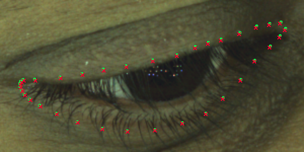
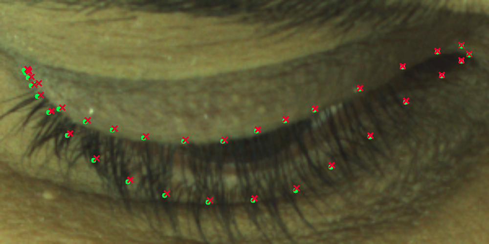
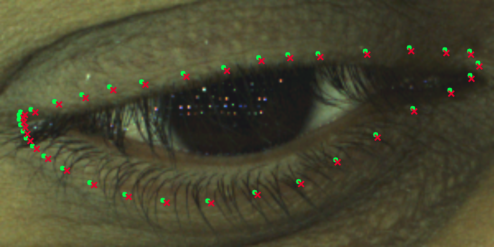
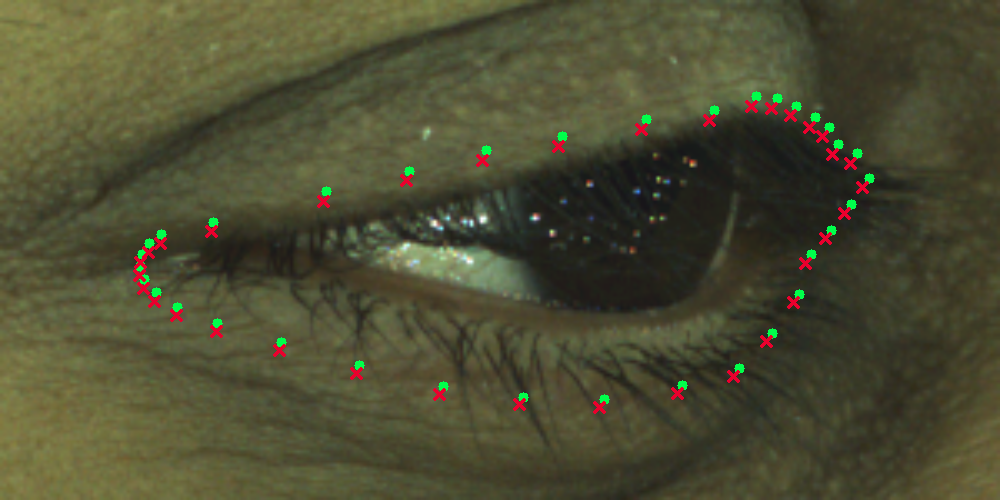
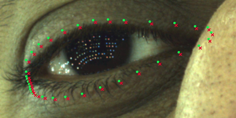
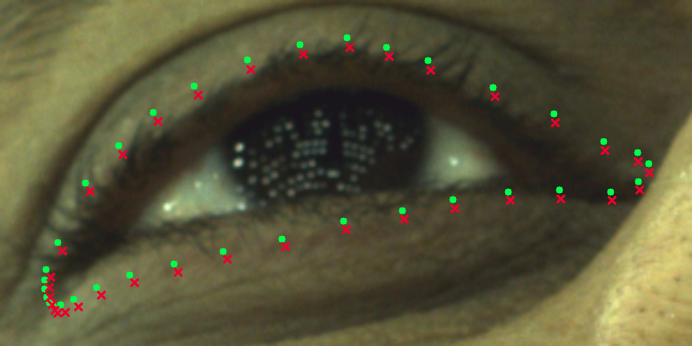
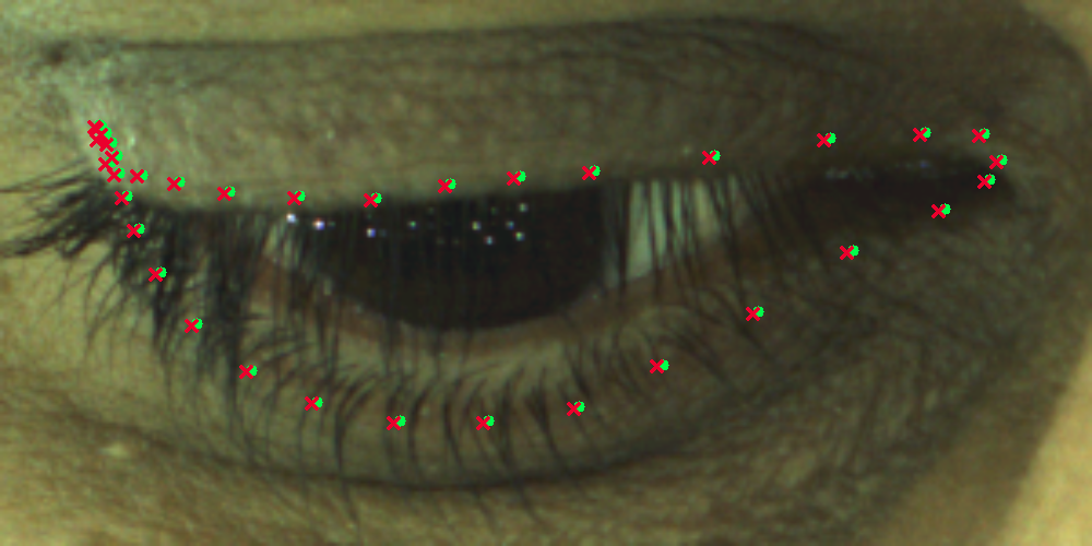
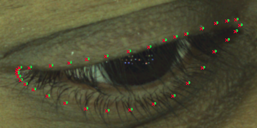
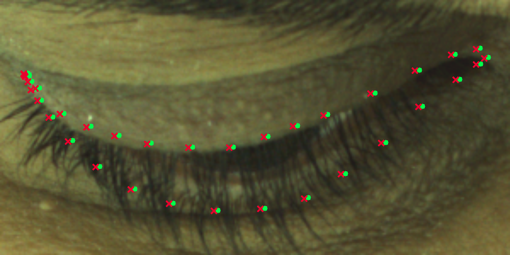
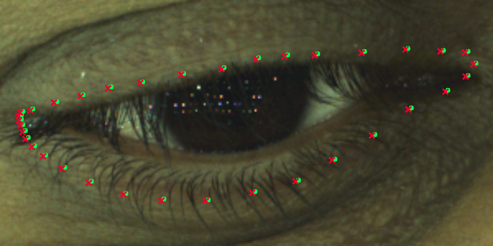
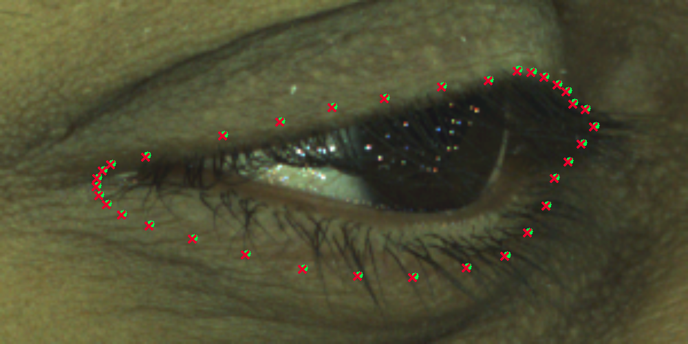
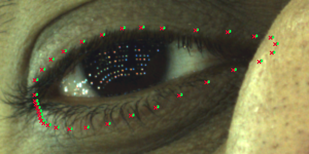
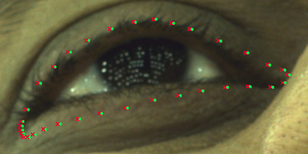
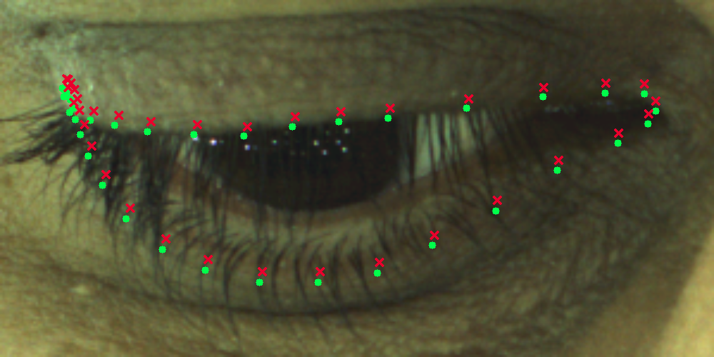
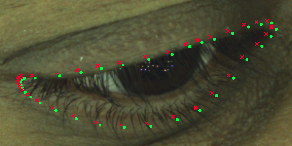
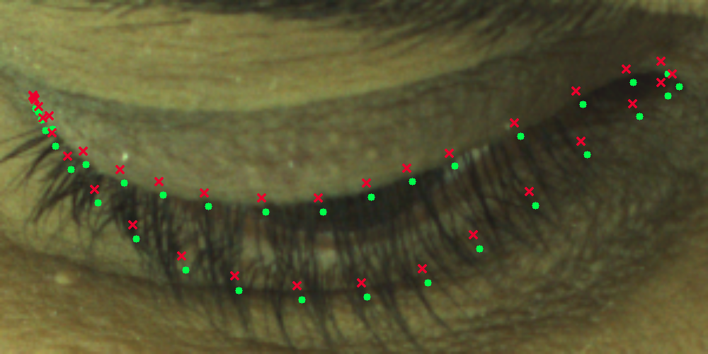
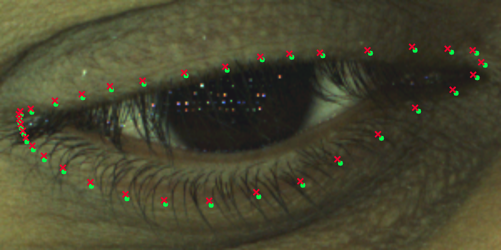
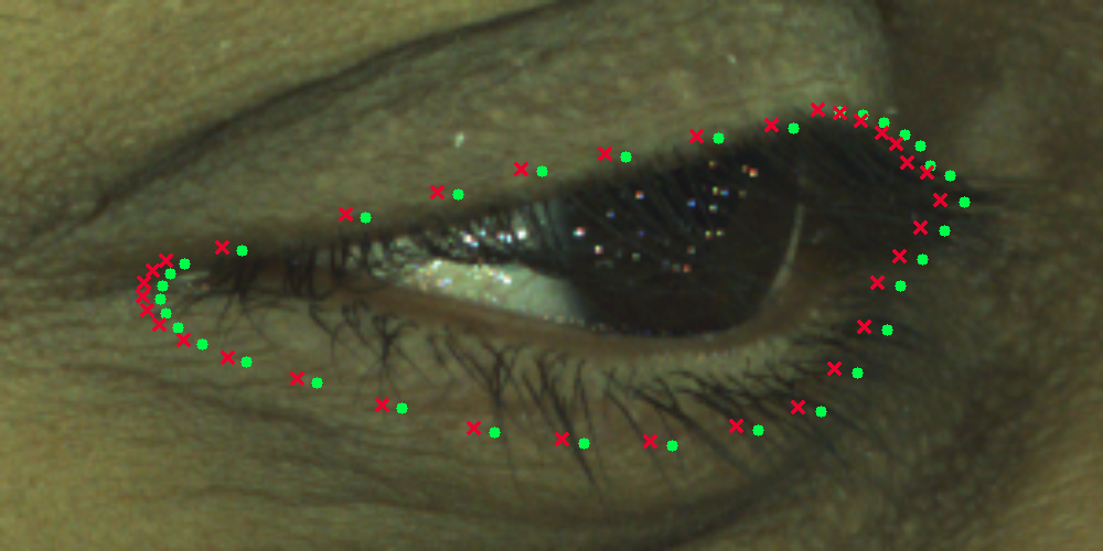
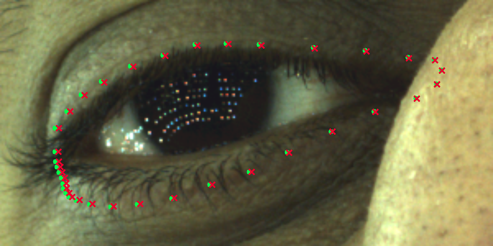
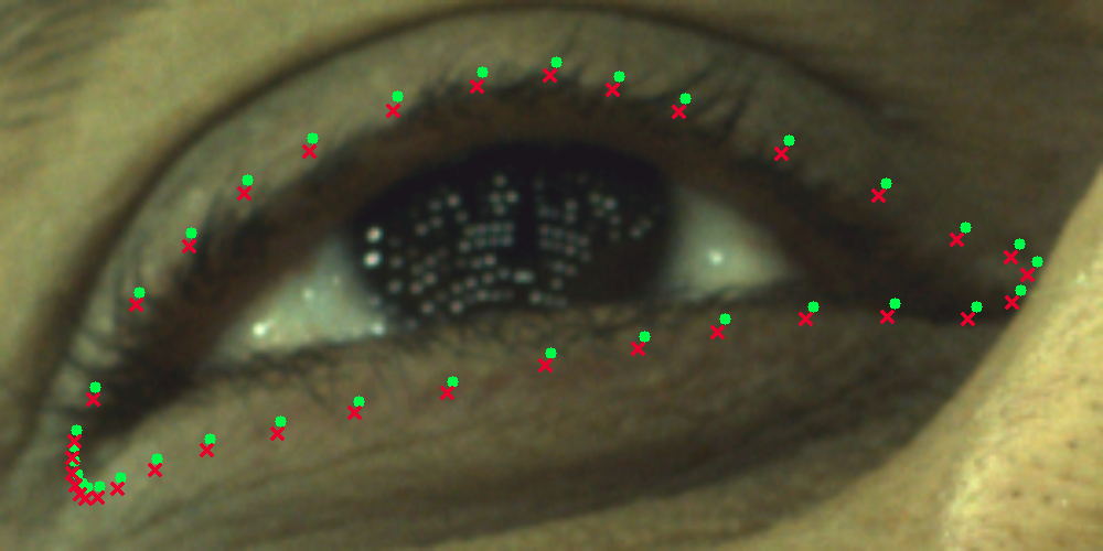
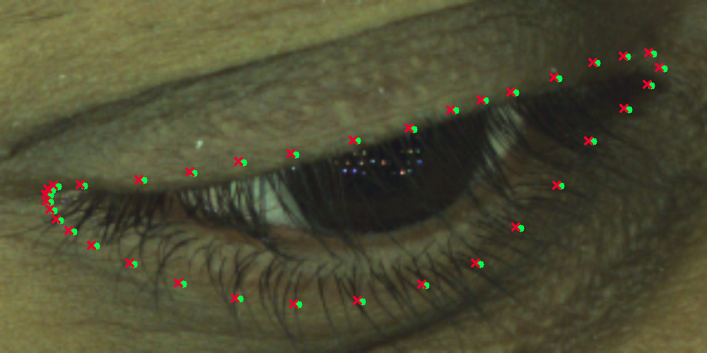
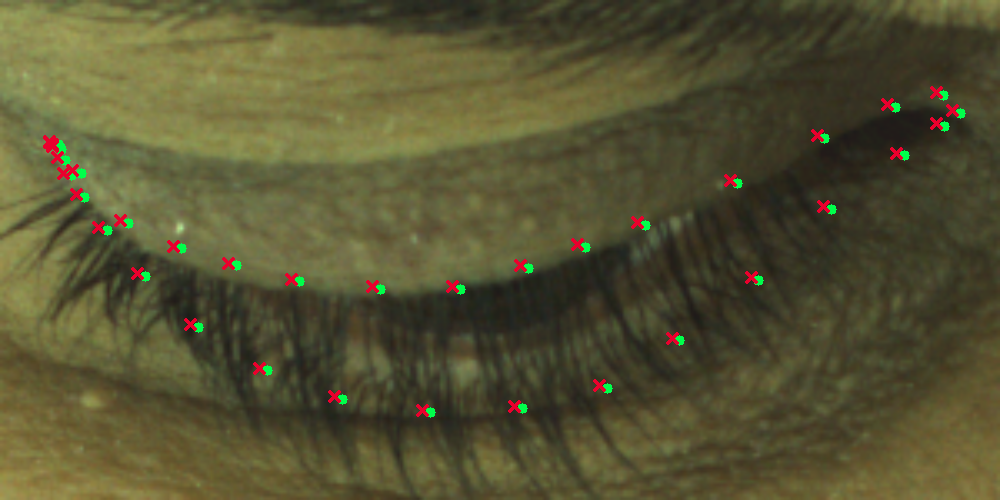
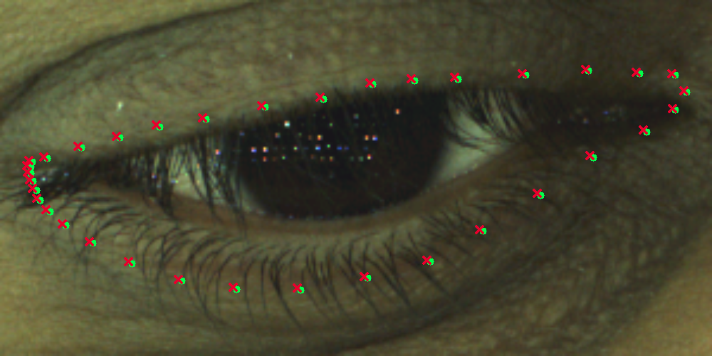
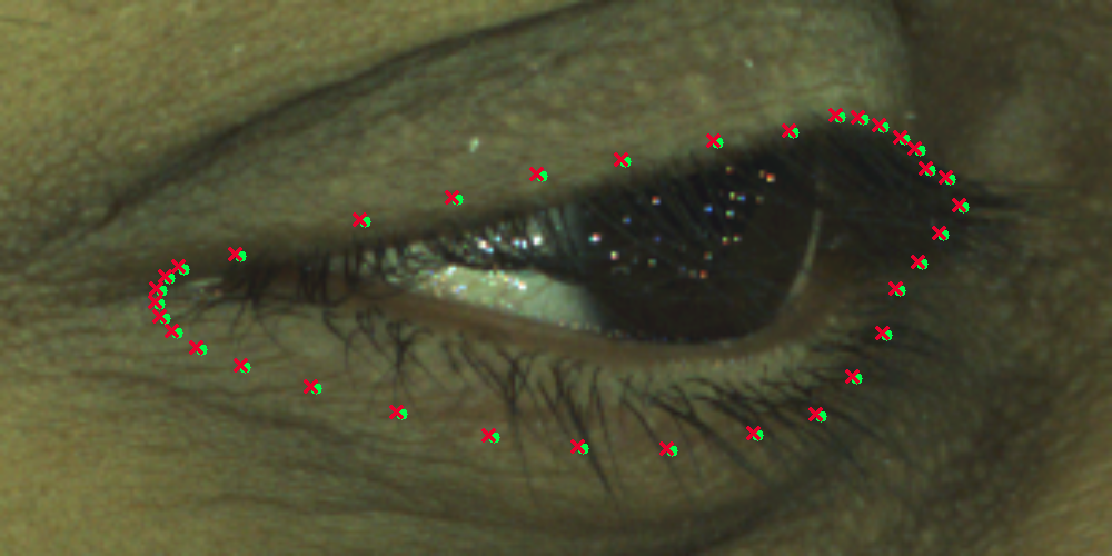
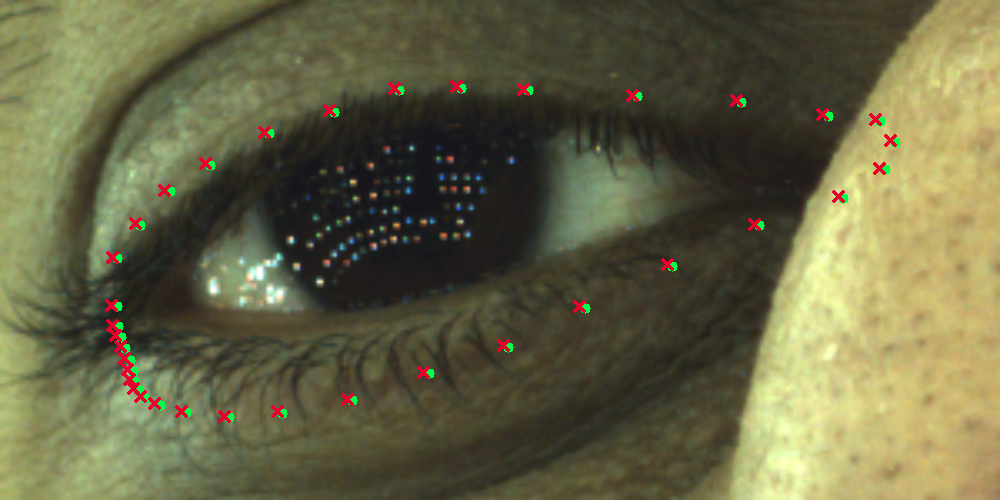
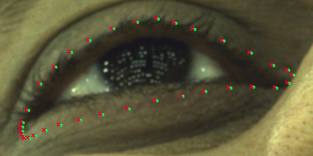
Fig. 2 visualizes reprojection errors for intrinsics estimated by COLMAP, Pixel-Perfect SfM, VGGSfM, and our method. We sample a few points on the ground-truth mesh and project them onto images using both ground-truth and estimated intrinsics. Our method achieves the smallest reprojection error.
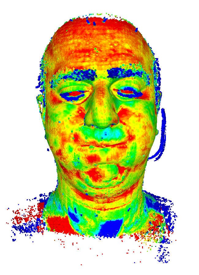
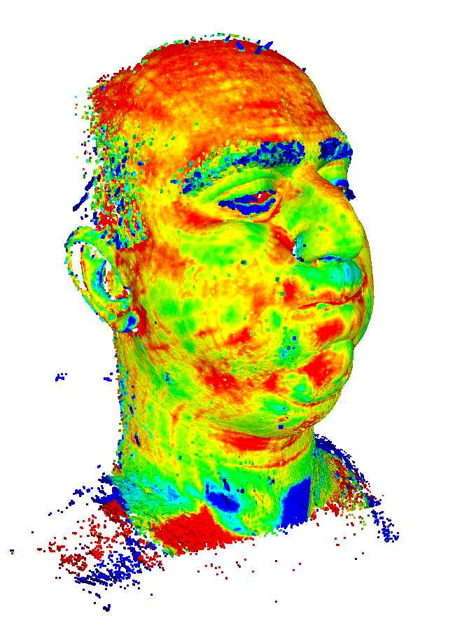
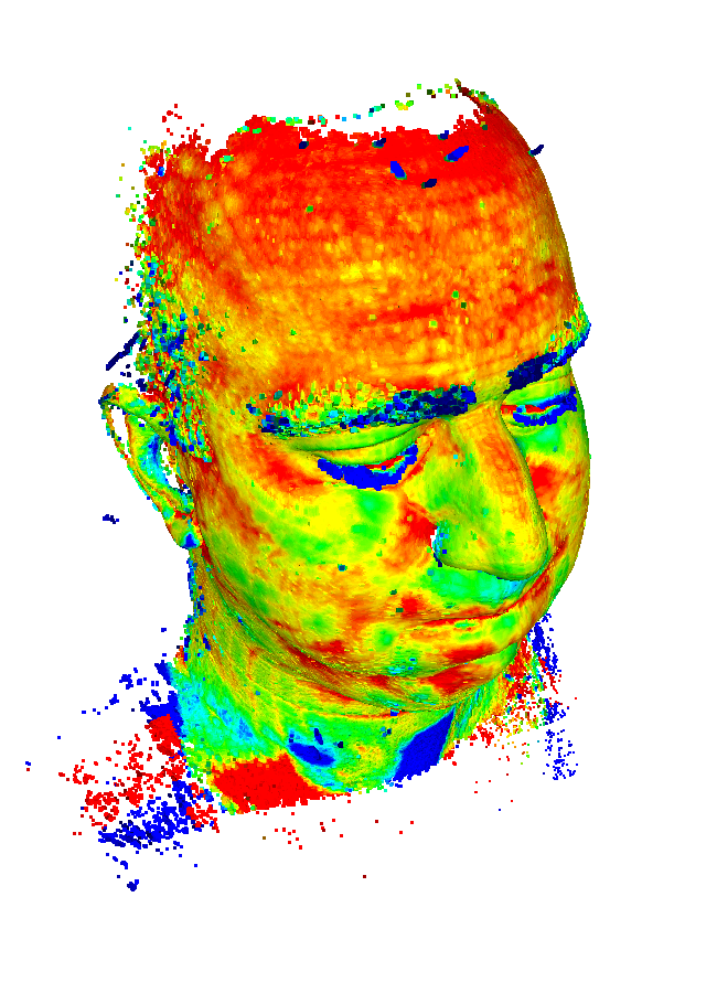
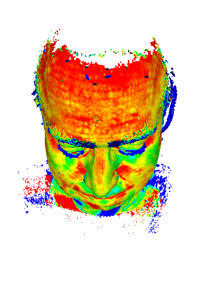
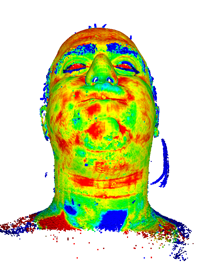
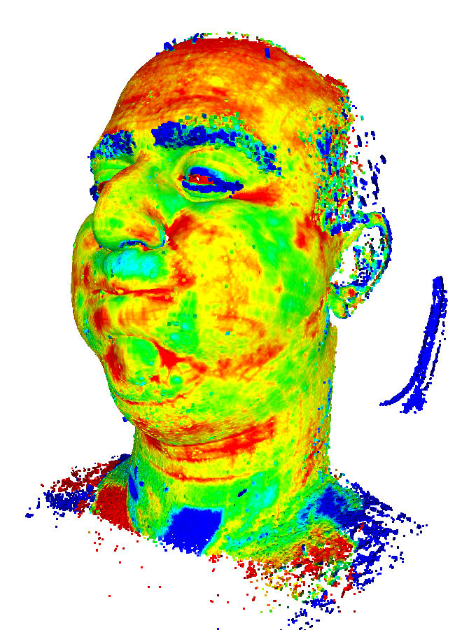
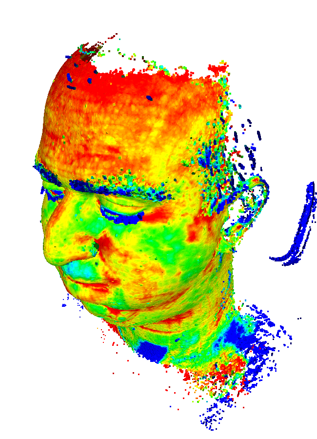
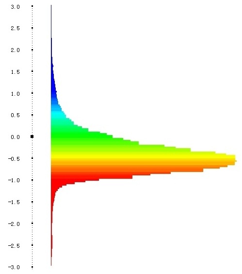
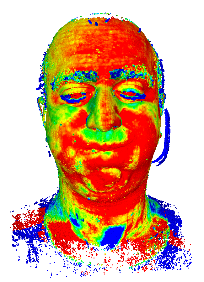
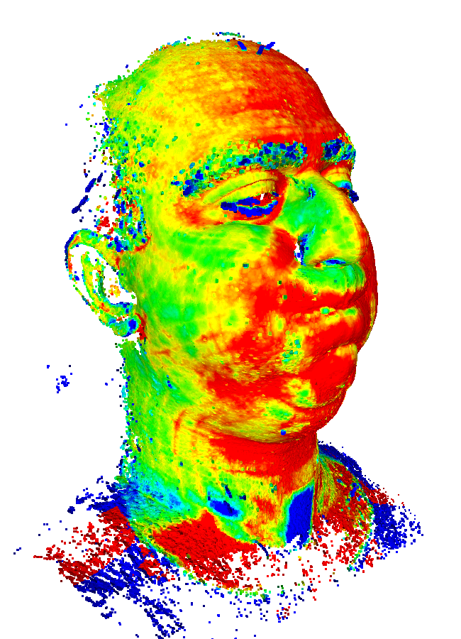
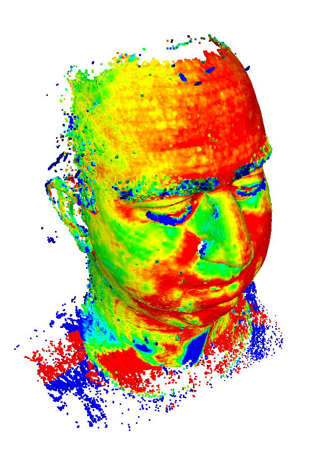
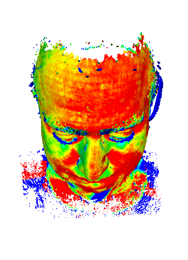
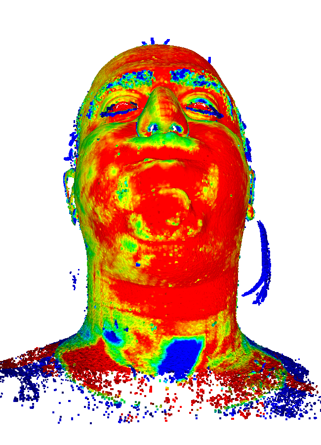
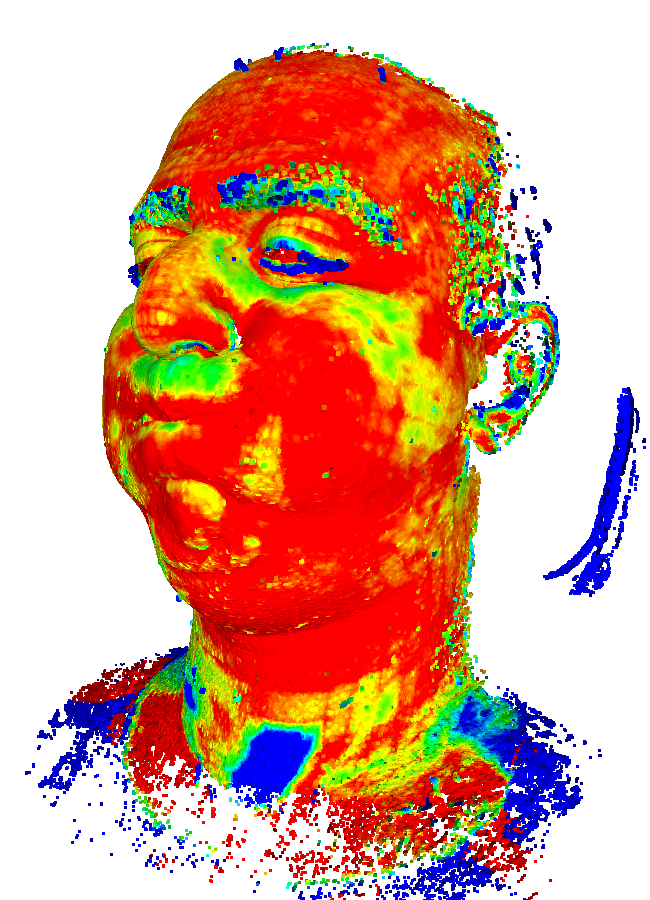
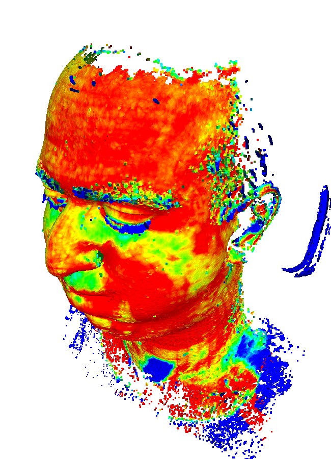
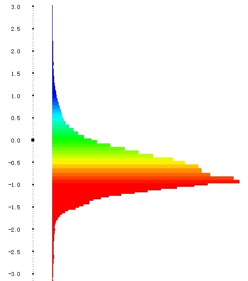
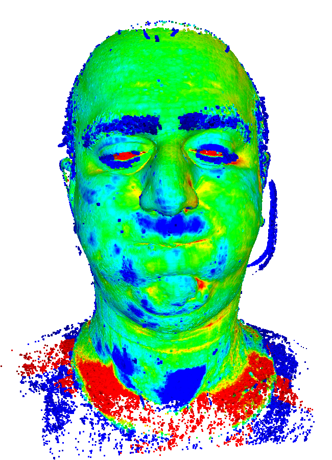
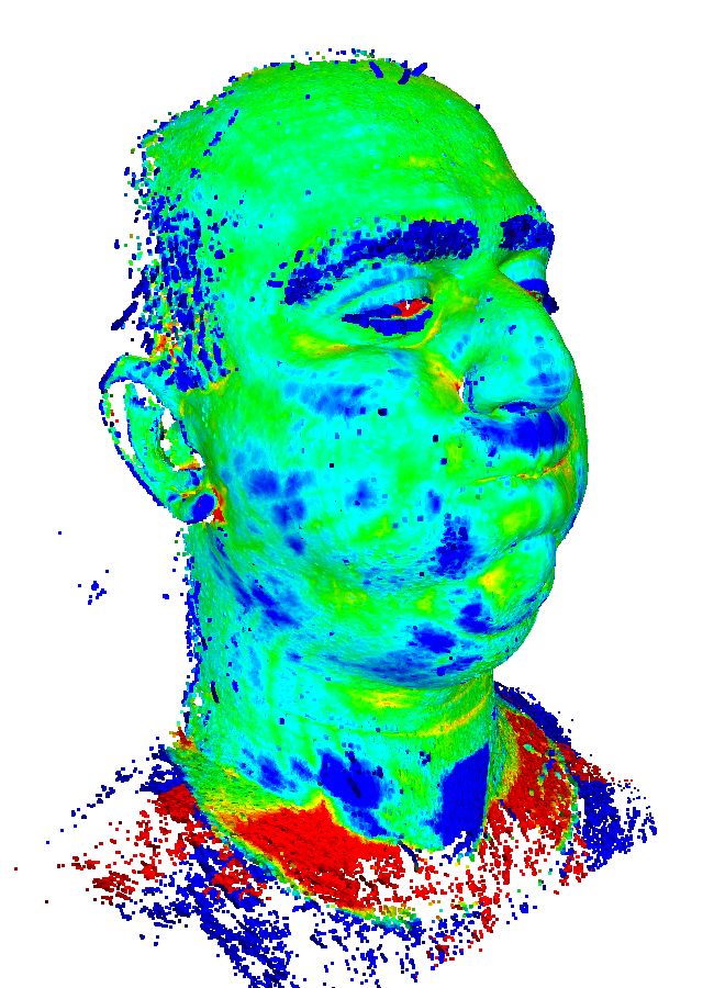
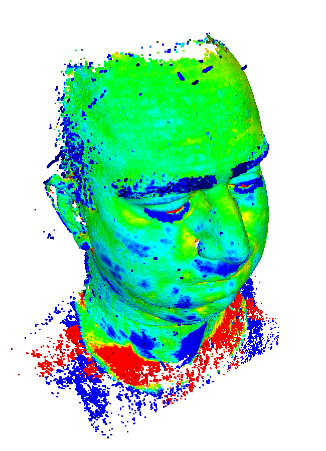
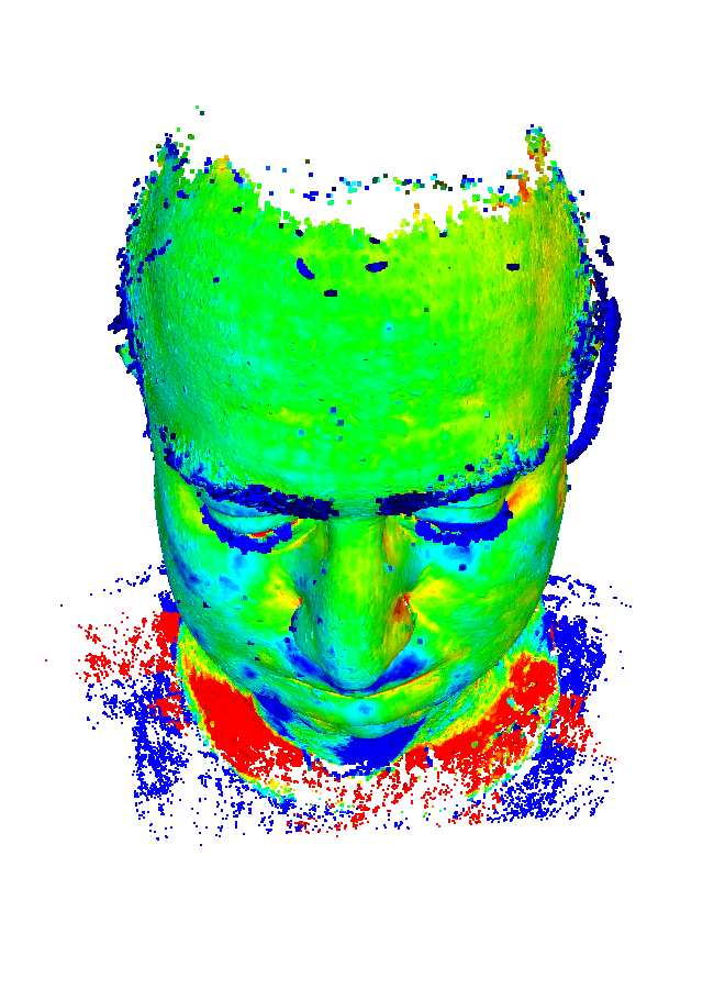
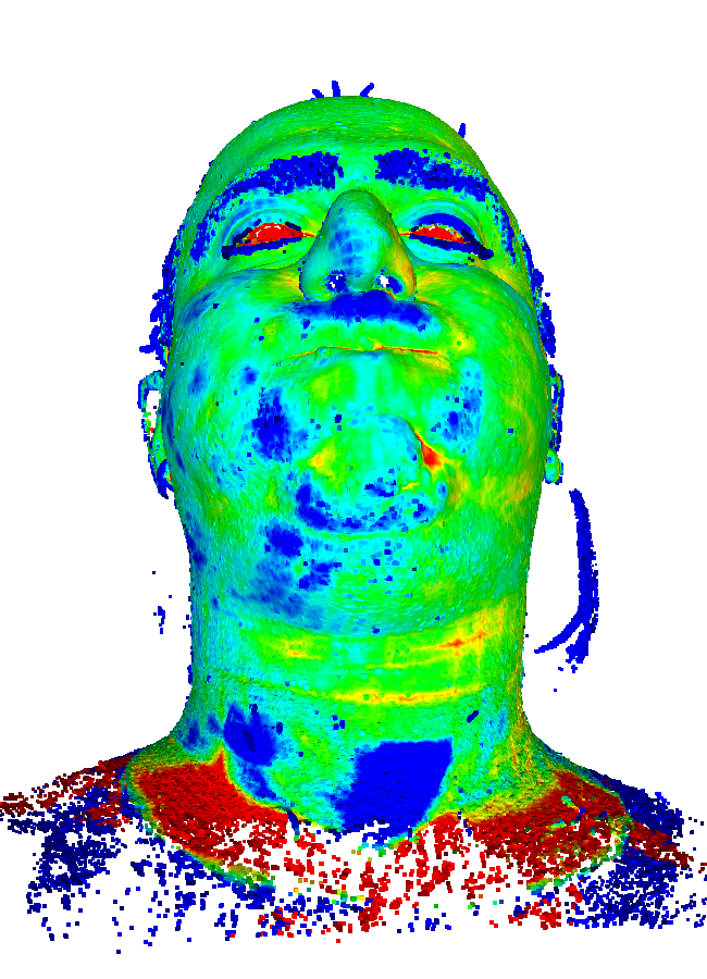
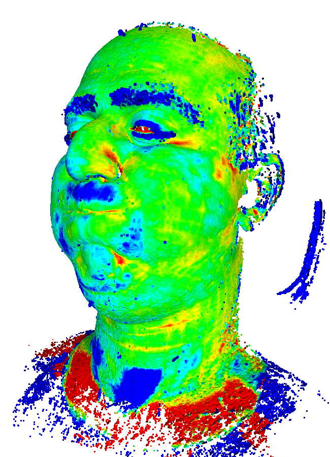
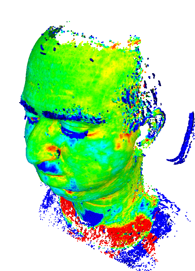
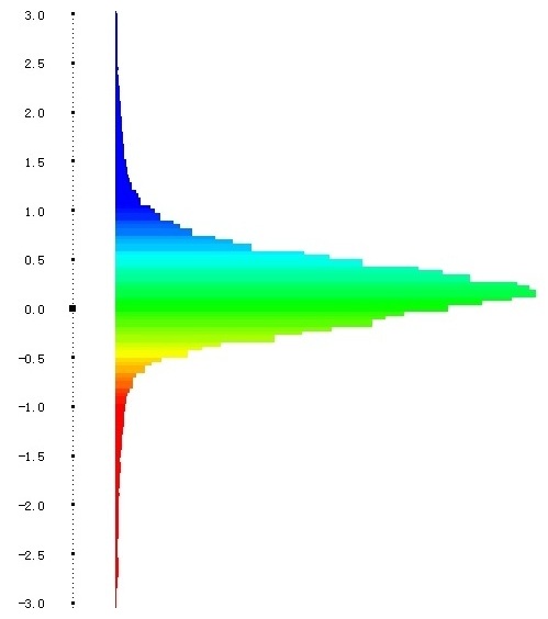
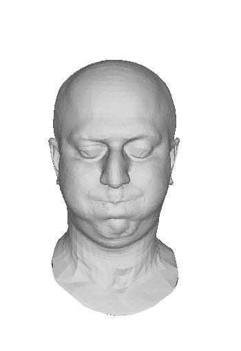
Fig. 3 compares multi-view stereo (MVS) reconstructions using COLMAP’s MVS pipeline with different intrinsics as input. We compute point-wise distances to the ground-truth mesh and visualize them in RGB colors, where blue represents positive errors, red indicates negative errors, and green denotes near-zero deviation. Our method exhibits a tighter concentration around green, demonstrating superior intrinsic accuracy compared to other methods.
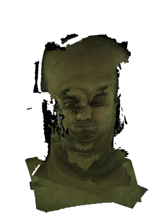
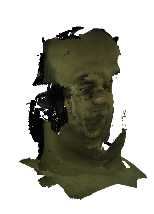
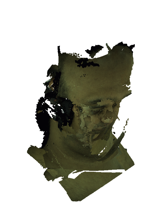
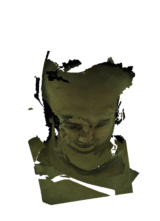
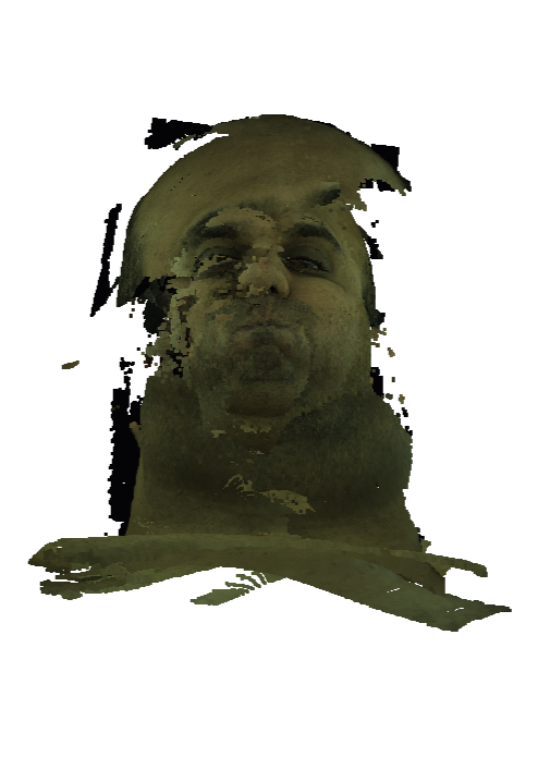
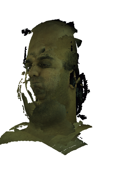
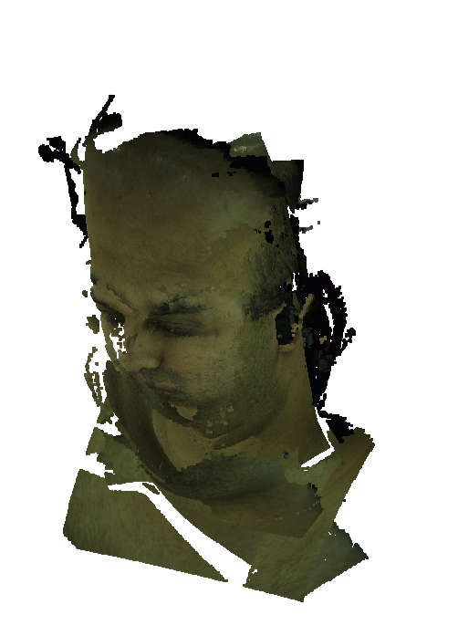
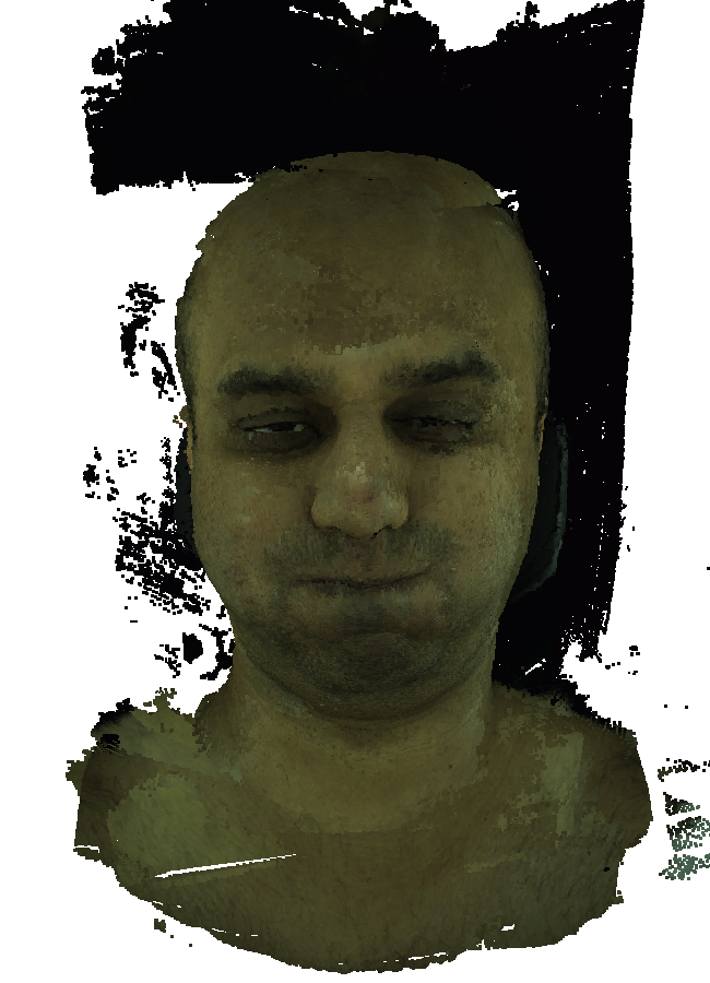
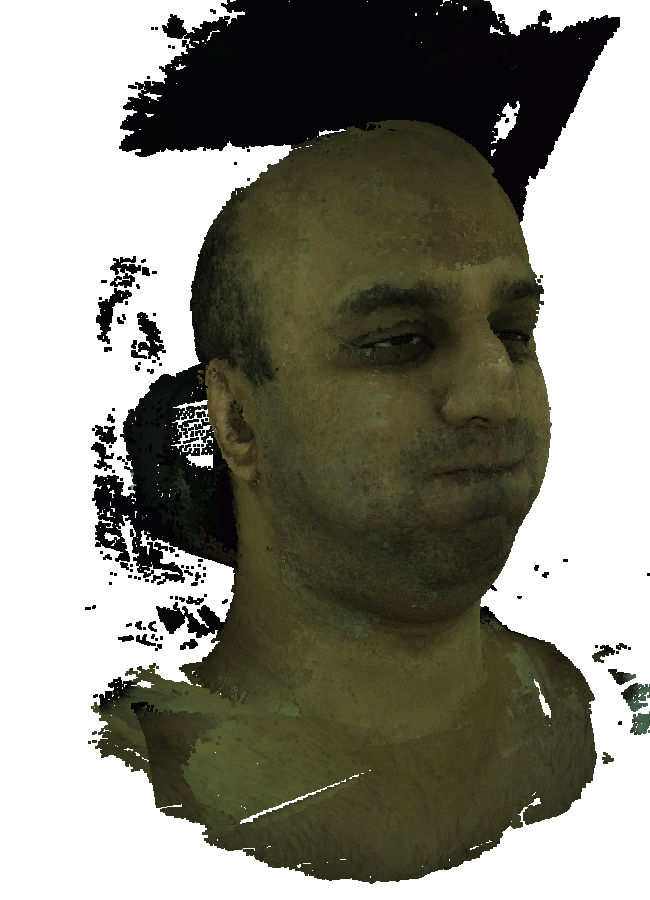
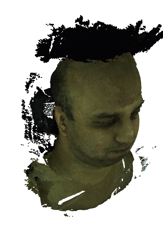
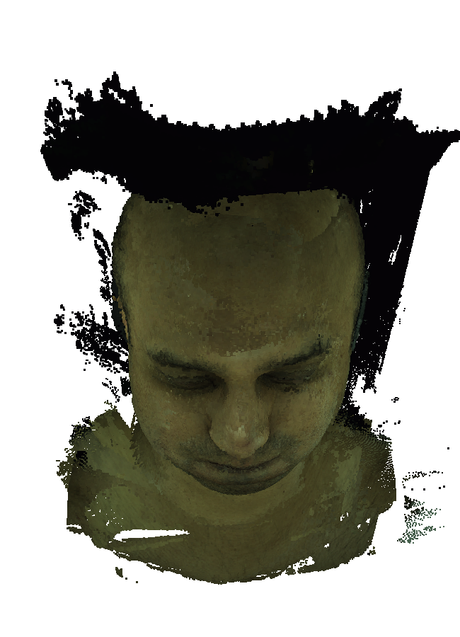
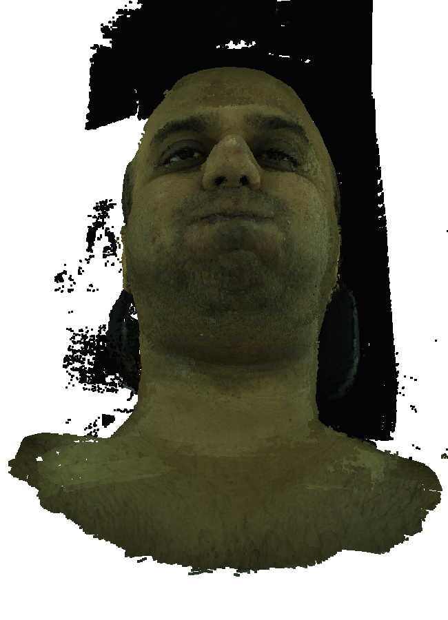
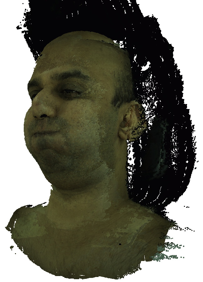
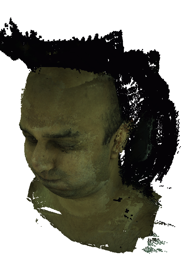
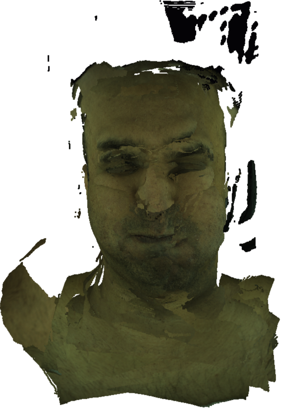
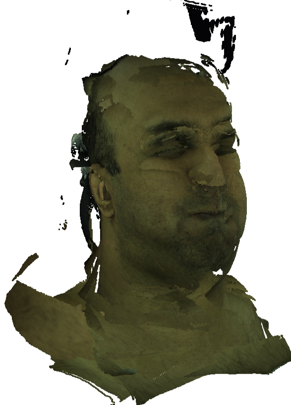
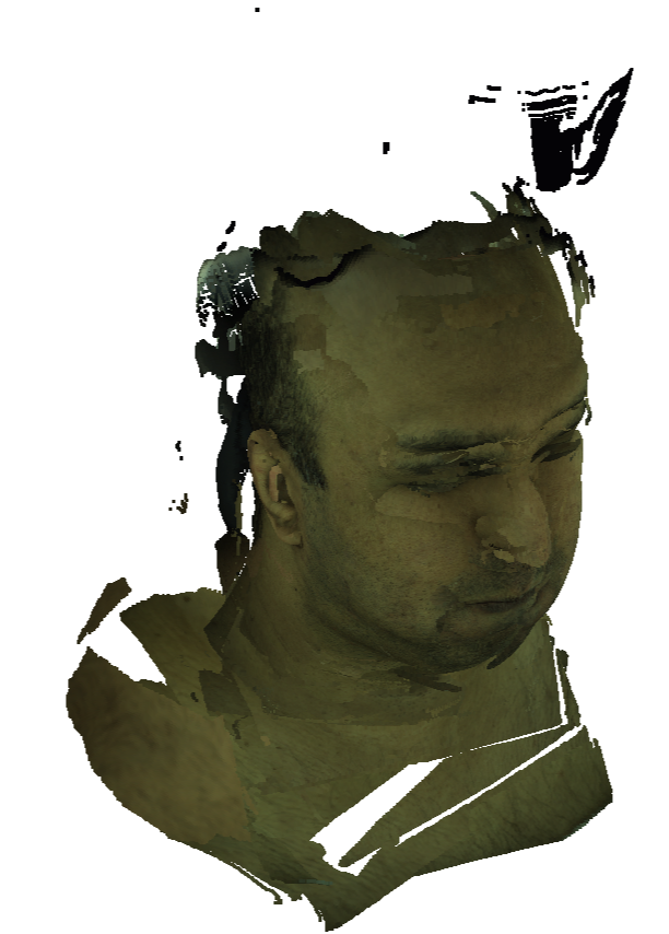
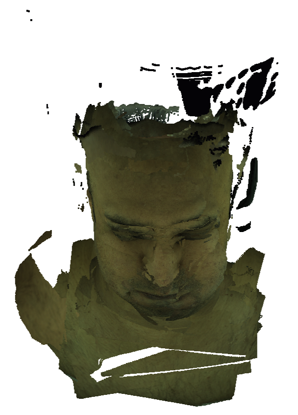
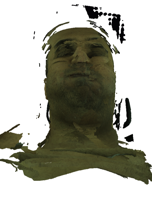
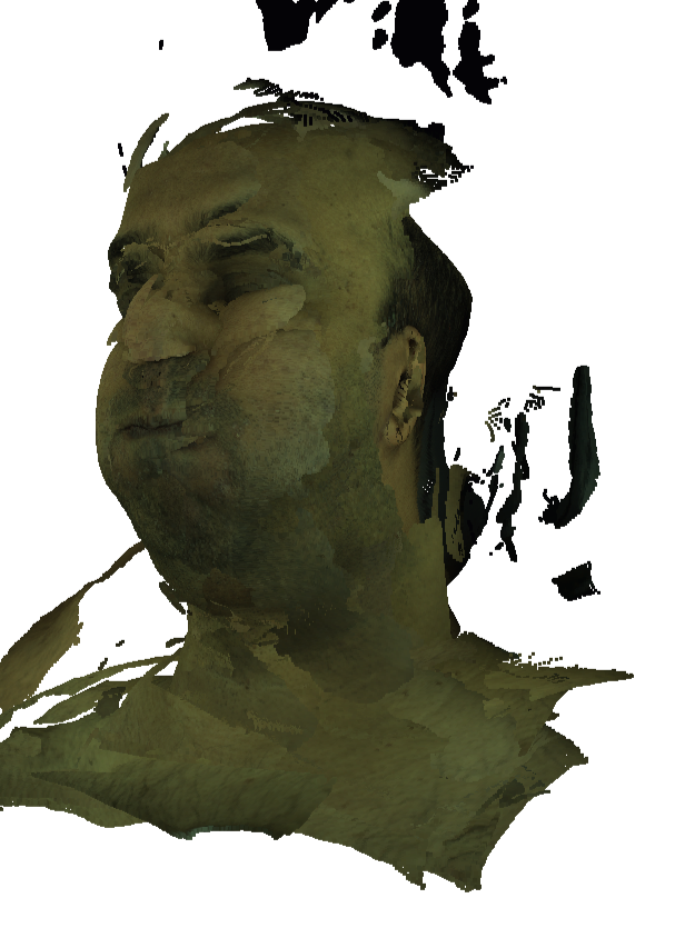
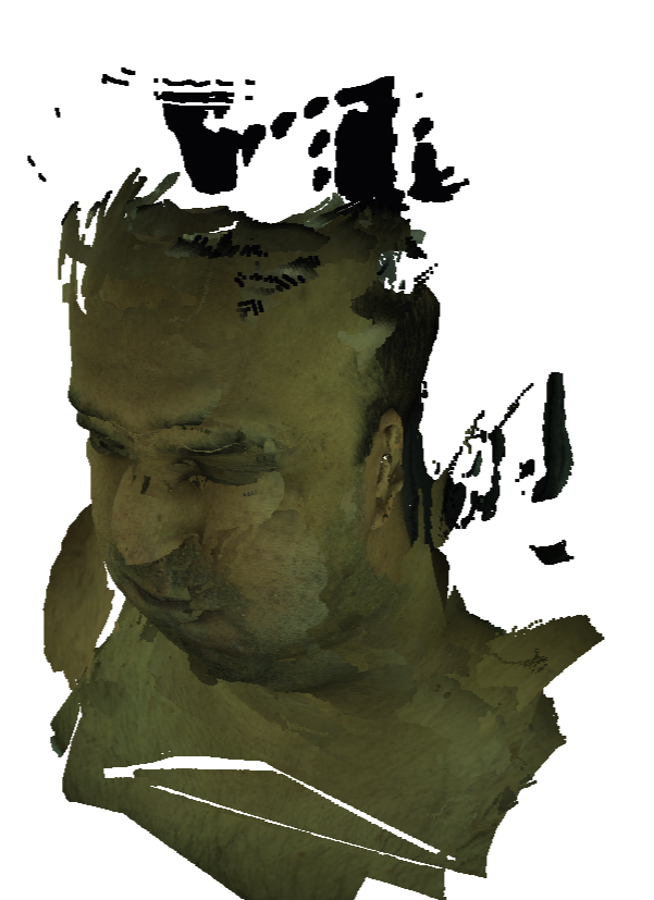
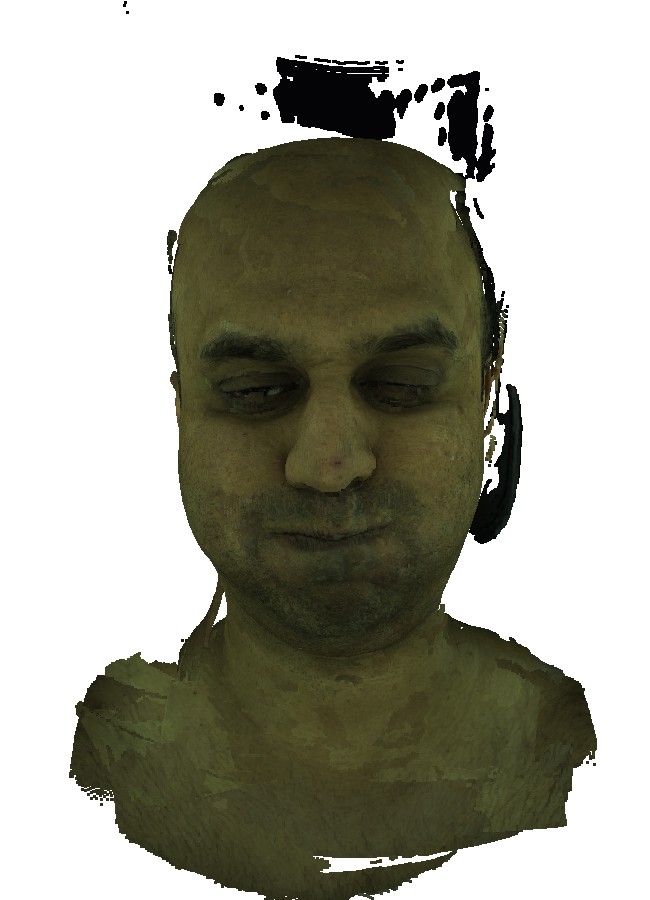
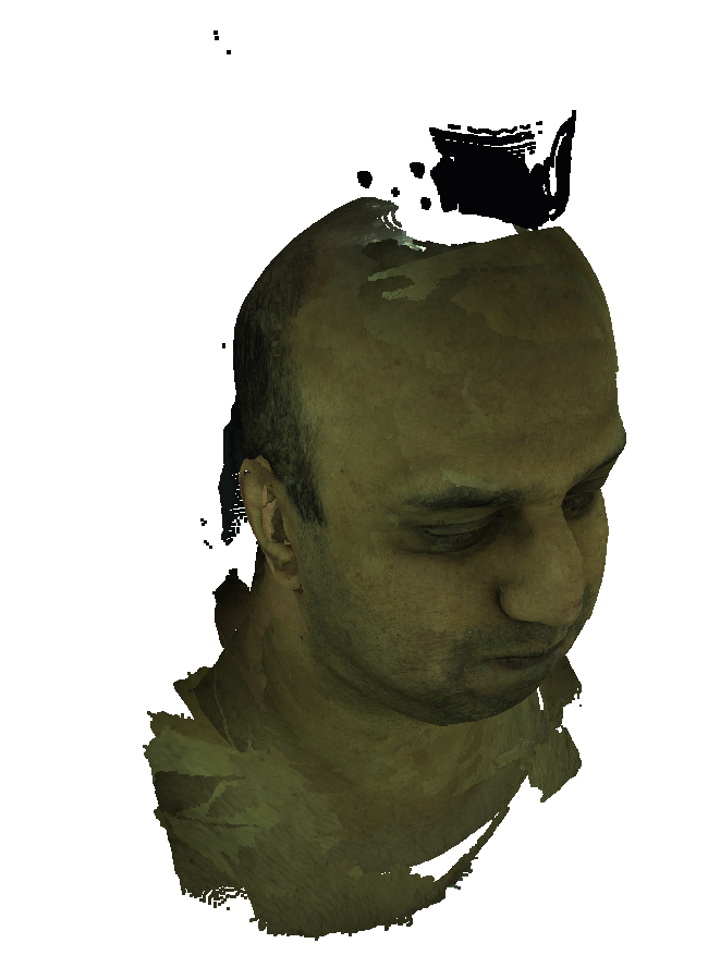
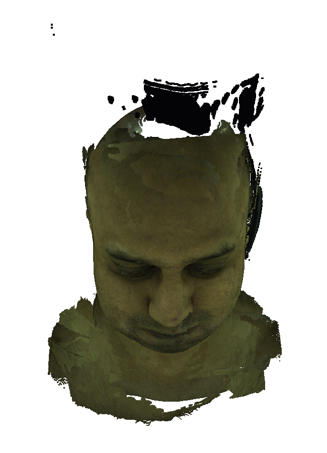
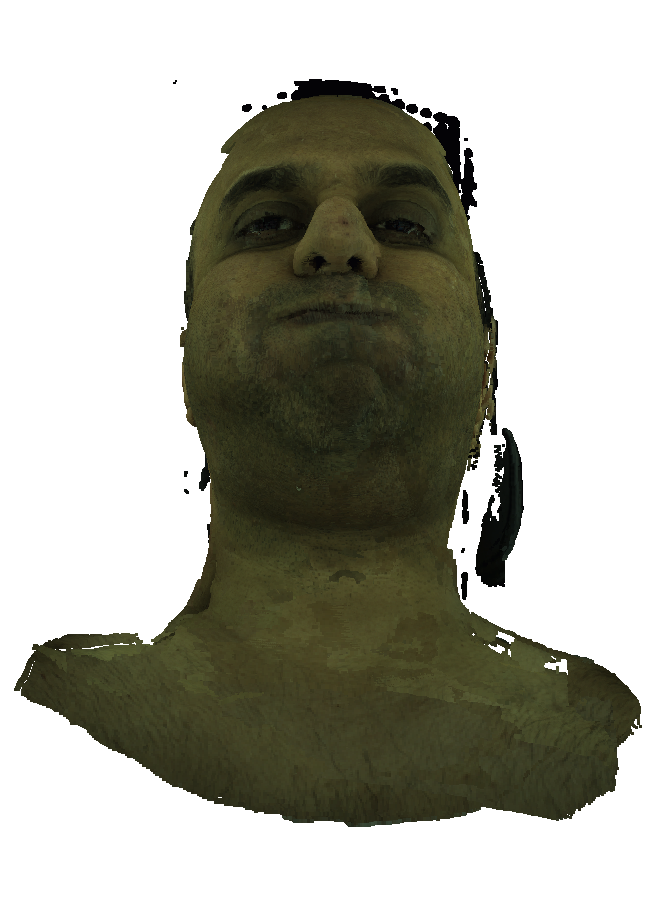
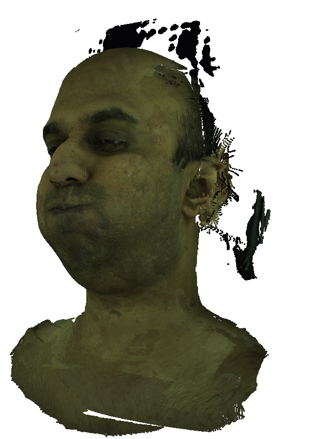
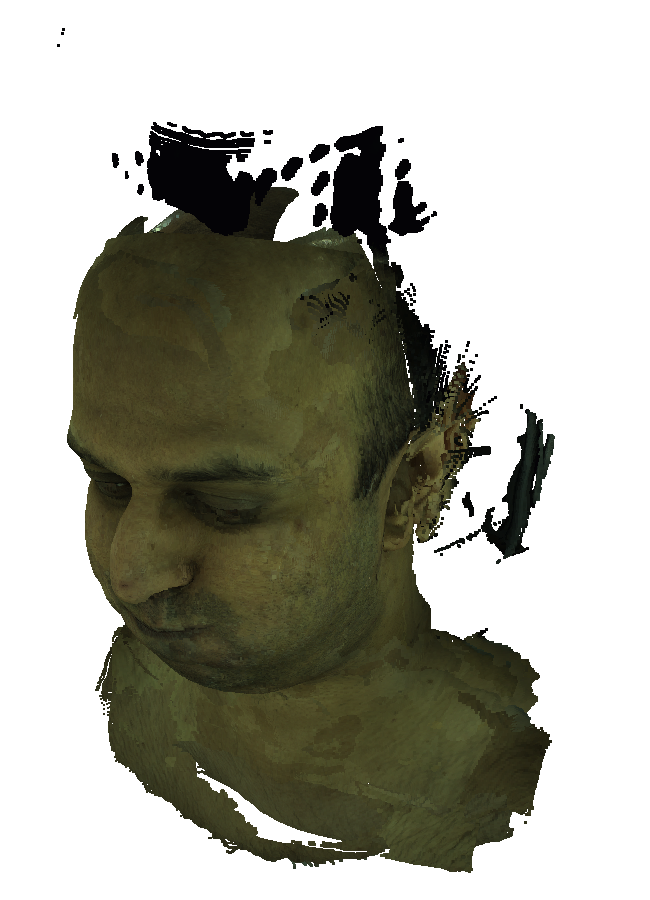
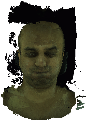
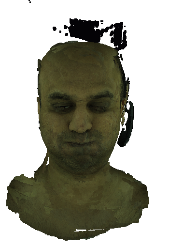
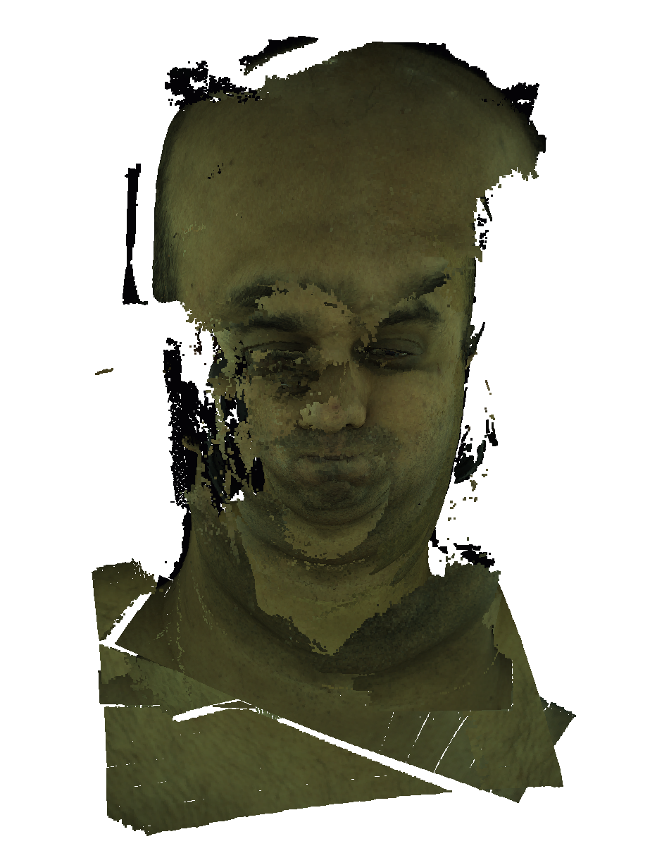
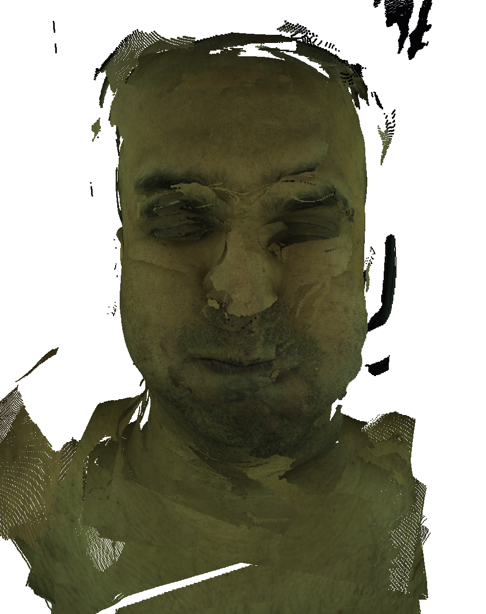
Additionally, we evaluate the effect of intrinsics on DUSt3R reconstructions, using its linear and DPT head models. We provide DUSt3R with ground-truth extrinsics but test two sets of intrinsics: (1) intrinsics estimated by DUSt3R and (2) intrinsics refined by our method. As shown in Fig. 4, the models using DUSt3R’s intrinsics exhibit large noise and depth inconsistencies, whereas models reconstructed using our refined intrinsics achieve more stable and accurate geometry. Moreover, because DUSt3R’s intrinsics significantly deviate from ground-truth, the reconstructed models differ in scale from the ground-truth mesh, as shown in Fig. 5.
IV-D Ablation Study
We conducted an ablation study to evaluate the impact of each component, as summarized in Table II. Starting with the baseline using only the reprojection term (Row 1), the absolute focal length and principal point errors are and , respectively. Adding the extrinsics regularization term (Row 2) slightly increases the focal length error, highlighting the importance of progressive coefficient adjustment. With this adjustment (Row 3), errors decrease to and . Including the dense feature reprojection term (Row 6) further reduces errors to and . Finally, adding the intrinsics variance term for multi-frame optimization (Row 7) achieves the best results, with absolute focal length error of and absolute principal point error of , showcasing the combined effectiveness of these components.
V CONCLUSIONS
We proposed a dense-feature-driven multi-frame camera calibration method for large-scale camera arrays. By proposing extrinsics regularization, dense feature reprojection, and intrinsics variance terms with multi-frame optimization, our approach achieves calibration-level precision without dedicated captures. Compatible with existing SfM pipelines, it offers an efficient solution for large-scale setups. For future work, we aim to further optimize computational efficiency for handling a large number of input frames and extend our method to accommodate more complex camera models, including cameras with lens distortions.
References
- [1] P. Lindenberger, P.-E. Sarlin, V. Larsson, and M. Pollefeys, “Pixel-Perfect Structure-from-Motion with Featuremetric Refinement,” in International Conference on Computer Vision (ICCV), 2021.
- [2] J. Wang, N. Karaev, C. Rupprecht, and D. Novotny, “Visual geometry grounded deep structure from motion,” arXiv preprint arXiv:2312.04563, 2023.
- [3] C.-h. Wuu, N. Zheng, S. Ardisson, and et al., “Multiface: A Dataset for Neural Face Rendering,” in arXiv preprint arXiv:2207.11243, 2022. [Online]. Available: https://arxiv.org/abs/2207.11243
- [4] M. E. Loaiza, A. B. Raposo, and M. Gattass, “Multi-camera calibration based on an invariant pattern,” Computers & Graphics, vol. 35, no. 2, pp. 198–207, 2011.
- [5] R. Usamentiaga and D. F. García, “Multi-camera calibration for accurate geometric measurements in industrial environments,” Measurement, vol. 134, pp. 345–358, 2019.
- [6] L. Huang, F. Da, and S. Gai, “Research on multi-camera calibration and point cloud correction method based on three-dimensional calibration object,” Optics and Lasers in Engineering, vol. 115, pp. 32–41, 2019.
- [7] G. Moreira, M. Marques, J. P. Costeira, and A. Hauptmann, “VICAN: Very Efficient Calibration Algorithm for Large Camera Networks,” in IEEE International Conference on Robotics and Automation (ICRA), 2024, pp. 18 020–18 026.
- [8] J. L. Schönberger and J.-M. Frahm, “Structure-from-motion revisited,” in The IEEE/CVF Conference on Computer Vision and Pattern Recognition (CVPR), 2016.
- [9] J. L. Schönberger, E. Zheng, M. Pollefeys, and J.-M. Frahm, “Pixelwise View Selection for Unstructured Multi-View Stereo,” in European Conference on Computer Vision (ECCV), 2016.
- [10] P. Moulon, P. Monasse, R. Perrot, and R. Marlet, “Openmvg: Open multiple view geometry,” in Reproducible Research in Pattern Recognition: First International Workshop, RRPR 2016, Cancún, Mexico, December 4, 2016, Revised Selected Papers 1, 2017, pp. 60–74.
- [11] H. Cui, X. Gao, S. Shen, and Z. Hu, “HSfM: Hybrid structure-from-motion,” in Proceedings of the IEEE conference on computer vision and pattern recognition, 2017, pp. 1212–1221.
- [12] L. Pan, D. Baráth, M. Pollefeys, and J. L. Schönberger, “Global structure-from-motion revisited,” in European Conference on Computer Vision. Springer, 2025, pp. 58–77.
- [13] S. Wang, V. Leroy, Y. Cabon, B. Chidlovskii, and J. Revaud, “Dust3r: Geometric 3d vision made easy,” in Proceedings of the IEEE/CVF Conference on Computer Vision and Pattern Recognition (CVPR), 2024, pp. 20 697–20 709.
- [14] D. G. Lowe, “Distinctive Image Features from Scale-Invariant Keypoints,” International Journal of Computer Vision, vol. 60, no. 2, pp. 91–110, 2004.
- [15] D. DeTone, T. Malisiewicz, and A. Rabinovich, “SuperPoint: Self-Supervised Interest Point Detection and Description,” in 2018 IEEE/CVF Conference on Computer Vision and Pattern Recognition Workshops (CVPRW), 2018, pp. 337–33 712.
- [16] J. Revaud, C. De Souza, M. Humenberger, and P. Weinzaepfel, “R2D2: Reliable and Repeatable Detector and Descriptor,” in Advances in Neural Information Processing Systems (NeurIPS), vol. 32, 2019.
- [17] M. J. Tyszkiewicz, P. Fua, and E. Trulls, “DISK: learning local features with policy gradient,” in Advances in Neural Information Processing Systems (NeurIPS), 2020.
- [18] P.-E. Sarlin, D. DeTone, T. Malisiewicz, and A. Rabinovich, “SuperGlue: Learning Feature Matching With Graph Neural Networks,” in IEEE/CVF Conference on Computer Vision and Pattern Recognition (CVPR), 2020, pp. 4937–4946.
- [19] H. Germain, G. Bourmaud, and V. Lepetit, “S2DNet: Learning Image Features for Accurate Sparse-to-Dense Matching,” in European Conference on Computer Vision (ECCV), 2020, pp. 626–643.
- [20] S. Seibt, B. Von Rymon Lipinski, T. Chang, and M. E. Latoschik, “DFM4SFM - Dense Feature Matching for Structure from Motion,” in IEEE International Conference on Image Processing Challenges and Workshops (ICIPCW), 2023, pp. 1–5.
- [21] J. Lee and S. Yoo, “Dense-SfM: Structure from Motion with Dense Consistent Matching,” in arXiv preprint arXiv:2501.14277, 2025.
- [22] X. He, J. Sun, Y. Wang, S. Peng, Q. Huang, H. Bao, and X. Zhou, “Detector-free structure from motion,” in Proceedings of the IEEE/CVF Conference on Computer Vision and Pattern Recognition (CVPR), 2024, pp. 21 594–21 603.
- [23] P. W. Holland and R. E. Welsch, “Robust regression using iteratively reweighted least-squares,” Communications in Statistics - Theory and Methods, vol. 6, no. 9, pp. 813–827, 1977.
- [24] S. Agarwal, K. Mierle, and T. C. S. Team, “Ceres Solver,” 10 2023. [Online]. Available: https://github.com/ceres-solver/ceres-solver