Time-Varying Causal Survival Learning
Abstract
This work bridges the gap between staggered adoption designs and survival analysis to estimate causal effects in settings with time-varying treatments, addressing a fundamental challenge in medical research exemplified by the Stanford Heart Transplant study. In medical interventions, particularly organ transplantation, the timing of treatment varies significantly across patients due to factors such as donor availability and patient readiness, introducing potential bias in treatment effect estimation if not properly accounted for. We identify conditions under which staggered adoption assumptions can justify the use of survival analysis techniques for causal inference with time-varying treatments. By establishing this connection, we enable the use of existing survival analysis methods while maintaining causal interpretability. Furthermore, we enhance estimation performance by incorporating double machine learning methods, improving efficiency when handling complex relationships between patient characteristics and survival outcomes. Through both simulation studies and application to heart transplant data, our approach demonstrates superior performance compared to traditional methods, reducing bias and offering theoretical guarantees for improved efficiency in survival analysis settings.
1 Introduction
In healthcare, understanding the causal effect of medical interventions on patient survival is crucial. Heart transplantation is a compelling example, as demonstrated by the Stanford Heart Transplant study (Crowley and Hu, 1977; Zhu et al., 2021), where patients with end-stage heart failure undergo surgery to replace their failing hearts with healthy donor hearts. While this procedure is likely to extend patients’ lives on average, researchers are particularly interested in how treatment effects vary with patient characteristics and surgical details. Time-to-event outcomes measure how long until a critical event occurs—in transplant cases, this is often the duration from surgery until death or organ rejection. Understanding these heterogeneous treatment effects—how the impact varies as a function of patient characteristics—is essential for improving patient selection criteria, optimizing intervention timing, and ultimately enhancing survival outcomes in transplant medicine (Trulock et al., 2007; Kilic et al., 2021; DeFilippis et al., 2022)
However, measuring the causal effect of such medical interventions is not straightforward. After a patient is listed as a candidate for heart transplant, they must wait for an available donor heart before undergoing the procedure (Almond et al., 2009). This means patients who receive heart transplants experience both control time (waiting period) and treatment time (post-transplant period). This differs from traditional causal inference where treatment and control groups are determined at the study’s outset and remain fixed throughout.
If there were a fixed time before which patients remained in the control group and after which they received treatment, then we could use that fixed time to separate treatment and control groups and conduct causal inference. However, this approach fails because treatment timing is random and highly variable. The waiting time for a heart transplant ranges from a few days to more than a year (Evans et al., 1986; O’Connell et al., 1992). The wide variation in treatment timing makes it impossible to establish any fixed time point that could meaningfully separate treatment and control groups (Akintoye et al., 2020).
Staggered adoption designs in econometrics (Athey and Imbens, 2022) provide a way to estimate causal effects with random treatment times. These designs compare outcomes between treated and yet-to-be-treated units, using later-treated units as controls for earlier-treated ones. While these designs work well for repeatedly measured continuous outcomes, where a unit’s outcome is obtained at different times (e.g., to study a policy’s effect on a country’s GDP, you obtain the country’s GDP over many years, with some observations before the policy and some after), they cannot handle time-to-event outcomes that are observed only once—either at the event occurrence (such as mortality) or at study end.
To address this challenge, we extend staggered adoption designs to time-to-event outcomes by integrating survival analysis techniques (Cox, 1972; Klein and Moeschberger, 1997; Fleming and Harrington, 2005; Kalbfleisch and Prentice, 2011). Specifically, we use hazard functions to model the instantaneous probability of an event. Hazard functions allow us to characterize each unit’s contribution to the outcome at any time, regardless of whether the unit is in its control or treatment period. We characterize a set of assumptions under which hazard-based models can be used to solve this causal inference problem.
In addition to handling random treatment timing, we address the complex, non-linear relationships between covariates and outcomes that often arise in real-world applications (Hastie et al., 2009). To handle these complexities, we employ double machine learning (DML) techniques (Chernozhukov et al., 2018; Künzel et al., 2019; Nie and Wager, 2021; Gao and Hastie, 2021) in our estimation procedure. DML provides a powerful framework for improving estimation efficiency, allowing us to flexibly model non-linear relationships while maintaining robustness to potential model misspecifications.
The contributions of this paper are twofold. First, we bridge the gap between staggered adoption designs and survival analysis by identifying conditions under which time-varying treatment effects can be estimated in a survival framework. Specifically, we show how key assumptions from staggered adoption designs can be adapted to justify the use of existing survival analysis techniques for causal inference with time-varying treatments. Second, we propose an estimator that addresses the complexity of real-world data, enhancing performance through Double Machine Learning (DML) techniques to ensure unbiased and efficient estimation of treatment effects, thereby advancing survival analysis methods for handling time-varying treatments.
1.1 Literature Review
Our work builds on survival analysis, staggered adoption literature, and heterogeneous treatment effect literature. While survival analysis provides tools for modeling time-to-event data and recent causal inference literature offers insights into time-varying treatments, the intersection—causal inference for survival outcomes with variable treatment timing—remains relatively unexplored. This gap needs attention because the problem is ubiquitous.
This methodological challenge extends beyond healthcare applications. In business settings, companies like streaming services and cloud storage providers need to understand how their interventions affect time-dependent outcomes. For example, when companies offer free membership trials, they must evaluate how free trial participation causally influences the time until conversion to paid memberships (Gopalakrishnan and Park, 2021; Almathami et al., 2024). As in transplant studies, both the timing of the intervention (free trial start) and the outcome (conversion) vary across units, making traditional causal inference methods insufficient for estimating these effects.
There have been several works combining causal inference with survival analysis. However, these approaches primarily focus on static treatments or simple time-varying confounders, rather than addressing the complexities of variable treatment timing. For example, Robins et al. (1992) and Hern’an (2010) introduced key methodological frameworks for causal inference in survival settings. Li and Greene (2015) developed doubly robust estimators for survival outcomes, while Zhang et al. (2017) proposed methods for handling time-dependent confounding. Vansteelandt and Joffe (2014) considered time-varying treatments, but in their work, treatment timing is well-defined, such as scheduled half-year visits for people with HIV, and treatment can be reversed. In contrast, our work considers treatments with stochastic timing that cannot be reversed.
The challenges of treatments with random timing have been extensively studied in the econometrics literature, particularly in the context of difference-in-differences designs. Recent work by Athey and Imbens (2022) and Goodman-Bacon (2021) has highlighted the importance of properly accounting for treatment timing in panel data settings. Sun and Abraham (2021) provided crucial insights into the bias that can arise from ignoring treatment effect heterogeneity across adoption cohorts. Imai and Kim (2021) further developed these methods for handling staggered treatment adoption. However, despite its importance, this crucial structure of random treatment timing remains largely unexplored in survival analysis settings, where our work pioneers new methodological approaches.
Our work employs Cox models for treatment modeling and focuses on learning the hazard ratio for survival outcomes, and this is different from other recent work on Cox models in causal inference. In related work, Shaikh and Toulis (2021) developed a framework for testing treatment effects in time-varying settings using Cox models, but they concentrate on testing the null hypothesis of no treatment effect on continuous outcomes. In the biomedical domain, Zhu and Gallego (2022) considered time-varying treatments in electronic health records, but their setting differs from ours in that the treatment depends on time-varying covariates at each point, rather than following a staggered adoption pattern.
For heterogeneous treatment effect (HTE) estimation with time-to-event outcomes, researchers have developed various machine learning approaches, though none have explicitly addressed the staggered adoption design. Cui et al. (2023) developed causal survival forests that adjust for right censored time-to-event outcome using doubly robust estimating equations, while Xu et al. (2024) proposed censoring unbiased transformations with orthogonality properties that can be integrated with existing HTE learners in scenarios with or without competing risks. Xu et al. (2022) provided a comprehensive review and tutorial on extending metalearners to handle right-censored time-to-event data. Taking a different approach, Gao and Hastie (2021) applied the double machine learning framework to exponential families, with Cox models serving as a specific instance. More recently, Wang et al. (2024) addressed estimation for left-truncated right-censored (LTRC) data, a significant advancement in the field. Despite these developments, the literature lacks methods specifically designed for causal inference in time-to-event settings with variable treatment timing as encountered in staggered adoption designs.
The organization of the paper is as follows: In Section 2, we formalize the notation, introduce assumptions for the causal framework, and present the statistical problem. In Section 3, we review existing methods for handling time-varying treatments in survival analysis. In Section 4, we introduce our double machine learning framework for robust estimation of heterogeneous treatment effects. In Section 5, we present simulation results demonstrating the performance of our method. In Section 6, we analyze the Stanford Heart Transplant dataset to evaluate treatment effect heterogeneity. Section 7 concludes with a discussion of our findings and limitations.
2 Problem Set Up
2.1 Notation and data
Let capital letters denote random variables and lowercase letters denote their realizations. Consider units. Let denote the time until an event of interest occurs, such as time until mortality in transplant studies. Each unit has a set of potential outcomes for , denoted as , where represents the date (or time) when a binary treatment is first adopted by the unit. We refer to this as the adoption date, consistent with the terminology used in the staggered adoption literature (e.g., Athey and Imbens (2022)). A unit can adopt the treatment at any of the time point , or not adopt the treatment at all during the time of observation, which we denote as . We take a super-population perspective of , i.e., are i.i.d. for some probability distribution , the choice of which is discussed below. We observe for each unit in the population the adoption date . The observed event time of interest is denoted as .
We also observe pre-treatment covariates . We adapt the following standard causal assumptions from Rubin (1974):
Assumption 1 (Stable Unit Treatment Value Assumption, SUTVA): Each unit’s potential outcome is determined solely by its own treatment assignment, with no interference between units and uniform treatment versions. For each unit ,
where the observed outcome equals the potential outcome under the assigned treatment. This assumption tells how potential outcomes map to observed outcomes. This also assumes everyone receives the same version of treatment in healthcare settings, which might not hold in practice—for example, surgical procedures may vary by surgeon expertise or hospital resources—so caution is warranted when applying these methods in real-world clinical scenarios.
Assumption 2 (Unconfoundedness): The treatment assignment is unconfounded, conditional on covariates . Formally,
meaning that the treatment assignment is independent of the potential outcome , given the covariates .
In healthcare settings, this assumption may hold when treatment decisions are based solely on observed patient characteristics that are included in our covariate set. For heart transplantation, this would require that all factors influencing both transplant decisions and survival outcomes—such as disease severity, comorbidities, organ compatibility, and functional status—are measured and accounted for in our analysis. However, this assumption could be violated if unobserved factors like physician preferences, hospital protocols, or patient preferences that aren’t captured in medical records influence both transplantation decisions and survival outcomes.
Assumption 3 (Overlap): The probability of receiving treatment at time , conditional on covariates, is strictly between 0 and 1 for all units. Specifically,
This assumption ensures that each unit has a non-zero probability of receiving either treatment or control. In healthcare systems, particularly for organ transplantation, this probability is often determined by allocation scores that rank patients based on observed covariates. For heart transplantation, factors such as blood type compatibility, tissue matching, disease severity, geographical proximity to donor, and waiting time all contribute to a patient’s position on the waiting list Cascino et al. (2022); Khush et al. (2013); Parker et al. (2019); Power et al. (2024). This structured allocation system means that the overlap assumption requires careful validation, as certain combinations of covariates might effectively determine treatment timing with near certainty.
2.2 Distributional Assumption and Introduction of Hazard
For the triplet of covariates, treatment, and outcome , we impose the following general distributional assumptions:
Here, represents the marginal density of the covariates on , without any additional parametric assumptions. The functions and denote conditional densities on , corresponding to the treatment and outcome, respectively.
We also need to account for censoring. Censoring occurs when the event of interest—in this case, patient mortality—is not observed for all units within the study period. The censoring time, denoted as , represents the time at which the unit’s data becomes unavailable for observation.
Censoring can arise for several reasons: a patient may be lost to follow-up, the study period may end before mortality is observed, or administrative reasons may prevent further observation. For censored units, the exact event time is unknown; we only know that it exceeds the censoring time . To handle this, we introduce a binary indicator variable , where indicates censored data and indicates fully observed event times. Thus, the observed data consists of covariates , treatment adoption time , observed time (the minimum of event time and censoring time), and censoring indicator . We can represent each unit’s data as the tuple .
When censoring is present, we cannot directly estimate the distribution of event times. Instead of using the probability density function (pdf) , we parameterize the distribution using the hazard function (Cox, 1972; Kalbfleisch and Prentice, 2011). The hazard function at time represents the instantaneous rate of event occurrence:
The hazard function is particularly useful for censored data because it characterizes the risk of an event at time , given survival up to that time. The relationship between the pdf and the hazard function is:
where is the pdf and is the cumulative distribution function (cdf). This relationship is one-to-one—specifying the hazard function uniquely determines the underlying distribution of the time-to-event variable (Klein and Moeschberger, 1997).
Note that for each fixed , the number of counterfactual hazard functions is infinite, as is continuous on . To address this complexity, we introduce two “exclusion” assumptions that simplify the model.
The first assumption states that the exact future transplant date doesn’t affect current outcomes (Abbring and Van den Berg, 2005; Abbring, 2008):
Assumption 4: No Anticipation
For all and for all adoption dates such that ,
This reduces the infinite set of potential distributions for to a single one by assuming that before treatment adoption, the outcome event follows the baseline (or control) hazard . In practical terms, this means that future treatment adoption does not influence current outcomes.
The second assumption asserts that conditional on treatment adoption, the magnitude of the adoption time does not matter for potential outcomes, but only whether adoption has occurred by time . This assumption is more restrictive but likely holds when a unit’s characteristics and event time have a stable relationship that does not change with exposure duration. However, this assumption might not hold when and have a dynamic relationship—for example, when the effectiveness of the transplant depends on how long the patient has had it, or when patient characteristics change significantly over time post-transplant.
Assumption 5: Invariance to History
For all and for all adoption dates such that ,
Together, assumption 4 and 5 enable us to simplify to only two hazard functions—one for the control, , and one for the treated, . These assumptions have been widely adopted in the Difference-in-Differences (DID) literature. For a comprehensive list of related works, see Section 3.2 in Athey and Imbens (2022).
We can now represent the hazard for the potential outcome, by the following:
| (1) |
where is a binary function that indicates whether treatment has begun at time .
We model the hazard using the proportional hazards model (Cox, 1972):
| (2) |
where represents the baseline hazard function, which captures the underlying risk of event at time when all covariates are at their reference levels. Reference levels here denote the baseline values of covariates (zero for continuous variables or the specified baseline category for categorical variables) that define the baseline hazard to which all other covariate combinations are compared. The functions and represent the proportional hazards for the control and treatment groups. These functions can be either linear or non-linear functions of the covariates. A key advantage of this model is its ability to decouple the time component, , from the covariate-dependent components, and . This leads to a simplified treatment effect definition where the time component cancels out:
| (3) |
We refer to this as the heterogeneous log hazard ratio (HLHR), which measures the treatment effect on the hazard rate for a patient with covariate profile .
In this paper, we assume that the treatment effect, , follows a linear parametric form. While more flexible specifications are possible, we focus on this linear specification for several reasons. First, in the context of heart transplant studies, key patient characteristics like age, medical history, and physiological measures often have approximately linear relationships with treatment outcomes (Choudhry et al., 2019). Second, this specification mirrors the successful progression in the causal inference literature, where initial work on heterogeneous treatment effects for continuous outcomes began with linear models before expanding to more complex specifications (Imai and Ratkovic, 2013; Kennedy, 2023). Specifically, for some , we model as:
| (4) |
As a result, the hazard function can be expressed as:
| (5) |
where is the baseline hazard and is an indicator function that denotes whether the treatment has been adopted by time .
To estimate , we proceed in two steps. First, in Section 3, we review existing partial likelihood methods in survival analysis that perform well when is correctly specified. These methods can achieve consistent estimation even when belongs to a complex function space. Then, in Section 4, we introduce our main contribution: a double machine learning framework that provides robust estimation of heterogeneous treatment effects even when is complex and potentially misspecified.
3 Review of Handling Time-Varying Treatment in Survival Models
In this section, we review the incorporation of time-varying variables in survival models, as discussed in Fisher and Lin (1999); Kalbfleisch and Prentice (2011).
3.1 Review of Partial Likelihood and Ordinary Cox Regression
We begin by revisiting the ordinary Cox regression model to guide the reader through the derivation of maximum partial likelihood. In this subsection, we assume treatment is fixed from the start. Under this assumption, the hazard function takes the form:
| (6) |
where represents the control group log hazard as a function of covariates , and is the treatment indicator.
The partial likelihood (Cox, 1972) is constructed by summing terms over the instances when an event (e.g., conversion) occurs, that is, when for a particular unit . Let denote the risk set for unit , representing the set of individuals who have not yet experienced the event at time . Furthermore, denote as the treatment status for individual . The log partial likelihood for the model is then expressed as follows:
| (7) |
To estimate the parameters and , we maximize this partial likelihood. This method is widely used in practice due to its robustness, as it does not require explicit specification of the baseline hazard function , while still maintaining desirable statistical properties (Andersen et al., 1993).
3.2 Review of Handling Time-Varying Treatment
To accommodate time-varying treatment, we replace the fixed treatment indicator with a time-varying indicator :
| (8) |
where indicates whether the treatment has been initiated by time .
To address the issue of time-varying covariates, we incorporate time variation into the partial likelihood framework (Fisher and Lin, 1999; Kalbfleisch and Prentice, 2011). This extension allows for the correct modeling of covariates that change over time.
We retain the risk set as defined previously. Let represent the treatment status of unit at time . The partial likelihood for this time-varying model is then expressed as:
| (9) |
This approach of incorporating time-varying treatments within the partial likelihood framework maintains desirable statistical properties and produces consistent estimators (Kalbfleisch and Prentice, 2011). Recent work by Tay et al. (2023) has extended this framework to allow lasso fitting when is non-linear.
While the above time-varying survival models provide a foundation for our work, they face challenges in consistently estimating treatment effects when the baseline hazard is misspecified. To address this limitation, we now turn to a double machine learning framework that provides robustness to model misspecification.
4 Double Machine Learning Estimator
We now focus on efficient estimation of the treatment effect function in the time-varying Cox proportional hazards model specified in Equation 6. As mentioned above, a straightforward approach would be jointly estimating and the baseline hazard using the pseudo-likelihood in Equation 9.
However, this direct approach faces significant challenges because the baseline hazard acts as a nuisance function, and its estimation can interfere with the consistent estimation of the treatment effect. Traditional outcome-based methods that rely on correctly specifying the outcome model (in this case, the hazard function) are particularly vulnerable in this setting. This vulnerability arises because misspecification of the baseline hazard can directly bias the treatment effect estimates through the partial likelihood structure—errors in estimating propagate non-linearly through the risk set calculations, leading to biased estimates of .
To address these challenges, we adopt a double machine learning (DML) framework (Chernozhukov et al., 2018; Künzel et al., 2019; Nie and Wager, 2021; Gao and Hastie, 2021). The key insight of DML is to introduce propensity score estimation alongside the outcome model, providing double robustness and improved convergence rates.
Under the DML framework, the treatment effect estimator achieves favorable convergence rates through the product of nuisance parameter estimation errors. More precisely, let be our time-varying propensity score as defined in Equation 10, and let be our baseline log hazard function as defined in Equation 6. If we denote the L2 convergence rates of their estimators as and respectively, then through careful orthogonalization of the score function, the treatment effect estimator satisfies:
Here, represents the rate at which our estimate of the propensity score converges to the true propensity score as sample size increases, while represents the rate at which our estimate of the baseline log hazard converges to the true function. These rates capture the statistical efficiency of our nuisance parameter estimators, with smaller values indicating faster convergence.
This product structure is crucial: even if one nuisance component converges at a slower rate (e.g., ), the treatment effect estimator can still achieve the optimal -rate of convergence as long as the other component converges sufficiently fast (e.g., ). This property, known as rate double robustness, makes the estimator robust to moderate misspecification of either nuisance component. For a comprehensive theoretical analysis of these convergence properties in the general framework of orthogonal statistical learning, we refer readers to Foster and Syrgkanis (2023).
4.1 Time-Varying Causal Survival Learner (TV-CSL)
Building upon the work of Gao and Hastie (2021), we propose TV-CSL (Time-Varying Causal Survival Learner) to handle time-varying treatments. The model is characterized by:
| (10) |
Here, represents the probability of adoption by time for non-censored data. This is analogous to the “treatment probability” or the propensity score at time . When all data is not censored, . The full estimation procedure is presented in Algorithm 1.
Our work differs from Gao and Hastie (2021), which developed a DML method for linear heterogeneous effects under a Cox model with treatment fixed at baseline, in two key aspects. First, the outcome models differ: their work uses the hazard form in Equation 6, while we use the time-varying form in Equation 8. Second, the propensity scores are distinct: their nuisance function maps covariates to probabilities in , whereas our propensity score is a function of both and , representing the cumulative distribution of adoption time conditional on .
4.2 Theoretical justification
Similar to existing causal inference literature (Nie and Wager, 2021; Künzel et al., 2019), we can derive theoretical results for the reduction of the learning rate.
Proposition 4.1 (Convergence Rate of Parameter Estimation).
Let the model for be denoted as . Under the following regularity conditions:
-
1.
The covariates are bounded, the true parameter lies in a bounded region , and the nuisance functions , along with their estimators , are uniformly bounded;
-
2.
The minimal eigenvalues of the score derivative 111See the Appendix C for a definition of the score in are lower bounded by some constant ;
If , , and , , then
| (11) |
Proof: See Appendix C
Proposition 1 states that for to reach a certain level of accuracy, the conditions on and are relatively loose. Specifically, if we want the estimate of to achieve convergence, we only need the product of the convergence rates of the outcome model and treatment model to be . For example, could converge at rate and at rate . In comparison, outcome-based methods that do not use the treatment model can only achieve convergence rate.
This result build upon the framework established by Gao and Hastie (2021). It has profound implications for causal inference in survival settings with random treatment timing. The assumptions underlying this proposition require that our covariates and parameters remain within reasonable bounds, ensuring stability in our estimation procedure. The second assumption about minimal eigenvalues ensures that our estimation problem is well-conditioned and that small changes in the data do not lead to disproportionately large changes in our parameter estimates. Together, these assumptions create a framework where we can achieve faster convergence by leveraging both the treatment and outcome models, even when each individual model might be estimated with moderate accuracy. This double robustness property is particularly valuable in healthcare applications like transplantation studies, where both the treatment assignment mechanism and the survival process are complex and difficult to model perfectly.
5 Simulation Study
In this section, we conduct comprehensive simulation studies to evaluate our method’s performance relative to existing approaches. We identify scenarios where our method demonstrates superior performance and conditions where its advantages are less pronounced, providing practical guidance for practitioners.
5.1 Simulation Design
Let denote the number of samples, and denote the baseline covariates for unit . , with sample sizes varies among . We generate baseline covariates from a multivariate normal distribution: where is a 33 identity matrix. The treatment time follows an exponential distribution with a rate parameter that depends linearly on covariates: .
The survival time is generated through a hazard function model where is a linear baseline hazard function, represents the baseline risk model, captures the heterogeneous treatment effect, and is the treatment indicator. Following Künzel et al. (2019), we specify the baseline risk model using a non-linear sigmoid-based function: with scaled sigmoid . The treatment effect is specified as a linear combination of covariates: . We implement random censoring with a maximum follow-up time of 20: , where . These parameters ensure approximately 75% of observations are non-censored, with the censoring mechanism independent of both outcome and treatment. The simulation was repeated 100 times for each scenario, with sample sizes to evaluate the properties of the finite sample.
5.2 Methods for Comparison
We evaluate two approaches for estimating heterogeneous treatment effects:
S-Lasso Method:222The name derives from ”S-learner” as referenced in Künzel et al. (2019); Nie et al. (2021), combined with our use of lasso regularization. This method employs a single regression combining baseline risk and treatment effect through additive specification. It is ”singly robust” as it does not incorporate the treatment model. For and specification, we consider two settings:
-
•
Linear specification: and
-
•
Complex specification: Includes natural splines, squared terms, and all pairwise interactions. Specifically, is linear in natural splines, squared terms, and all pairwise interactions of , and is linear in natural splines, squared terms, and all pairwise interactions of multiplied by . This results in a substantially larger feature space that captures non-linear relationships and interaction effects between predictors. While this more flexible specification can model complex relationships more accurately, it comes with increased risk of overfitting and reduced interpretability compared to the linear specification. The choice between these specifications represents a classic bias-variance tradeoff.
The combined model is fit using Lasso regularization with cross-validated penalty parameter.
TV-CSL Method: This is our proposed doubly robust estimation through cross-fitting in two stages:
-
•
First stage estimates the treatment model under both correct (all covariates) and misspecified (single covariate) settings
-
•
Second stage estimates the baseline outcome model using Lasso with specifications matching S-Lasso
The Performance is evaluated using empirical Mean Squared Error (EMSE):
where this calculation is performed on an independently generated testing set to evaluate out-of-sample performance. The MSE measures estimation quality by capturing both bias and variance components. All reported values are averages across 100 simulation replications.
5.3 Results
Our simulation results demonstrate the relative performance of TV-CSL and S-Lasso under various specifications, focusing on estimation accuracy and robustness to model misspecification. We examine two key aspects: the impact of the treatment model specification and the performance under complex treatment effect specifications.
5.3.1 Effect of Treatment Model Specification
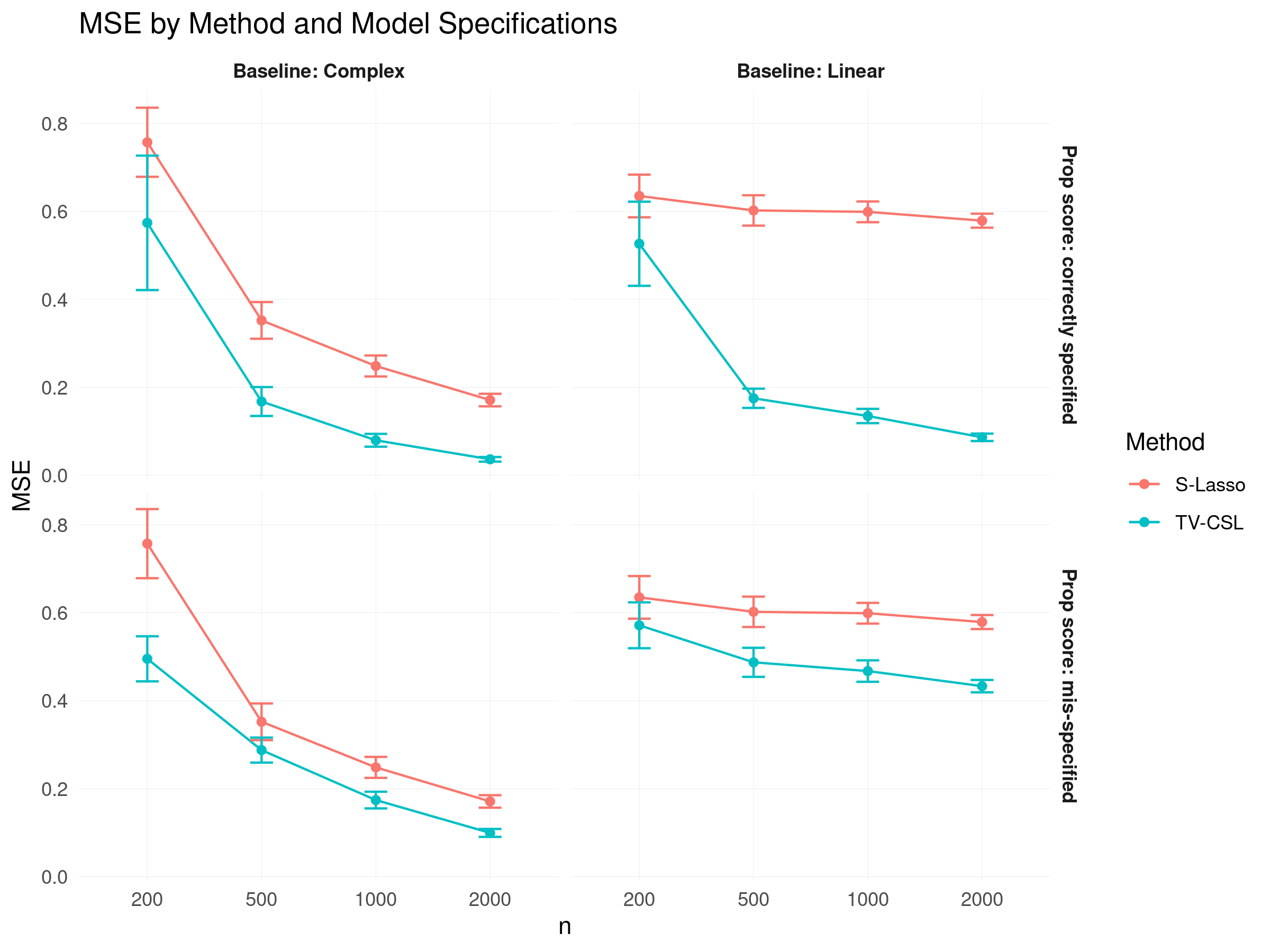
We first examine how the treatment model specification affects estimation quality. To isolate this effect, we maintain a correctly specified HTE model to ensure optimal conditions for both methods.
The results are shown in Figure 1. Both methods achieve lower MSE with the complex baseline outcome specification, which aligns with the true data-generating process where the baseline hazard () follows a non-linear pattern.
Comparing TV-CSL and S-Lasso, we observe that TV-CSL consistently outperforms S-Lasso regardless of treatment model specification, with the performance advantage being more pronounced when the treatment model is correctly specified. This aligns with our theoretical findings that the convergence rate depends on the product of errors in the nuisance estimators.
Notably, TV-CSL maintains its advantage over S-Lasso even when the treatment model is misspecified. This robustness can be attributed to the simplicity of our treatment model, where minor misspecifications have limited impact on the overall estimation error. The double machine learning framework effectively mitigates the impact of treatment model misspecification, allowing TV-CSL to maintain robust performance.
5.3.2 Performance Under Complex Treatment Effect Specifications
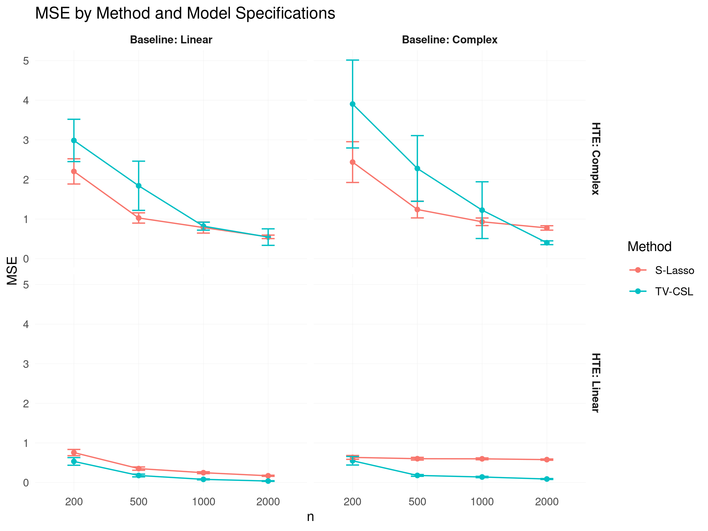
While our previous analysis focused on a linear (correctly specified) HTE model, we now evaluate the performance when using a complex model to estimate the HTE. Figure 2 presents these results.
For both methods, holding the outcome model fixed, the use of complex HTE specifications leads to higher MSE, though the magnitude of this increase varies between methods. This increased error can be attributed to the additional complexity in estimating the treatment effect model.
TV-CSL demonstrates superior performance relative to S-Lasso under two conditions: First, when the HTE model is correctly specified as linear, TV-CSL consistently outperforms S-Lasso across all sample sizes. This advantage stems from the double machine learning framework’s ability to reduce the impact of nuisance parameter estimation errors. Second, for complex HTE specifications, TV-CSL’s performance shows strong sample size dependency. While maintaining comparable performance at smaller sample sizes, TV-CSL outperforms S-Lasso at larger sample sizes.
6 Data Analysis – Stanford Heart Transplant dataset
The Stanford Heart Transplant dataset originates from the pioneering efforts of the Stanford Heart Transplantation Program, which began in the 1960s. The program aimed to extend the lives of patients suffering from severe heart conditions by providing them with heart transplants. Patients were admitted based on strict medical criteria, and donor hearts were matched primarily by blood type. The dataset tracks patient survival times from program acceptance through three key phases: the initial enrollment period, the waiting period for a suitable donor heart, and the post-transplant period. The primary goal is to evaluate how heart transplants affect patient survival, while accounting for various patient characteristics such as age and previous surgical history (Crowley and Hu, 1977).
In our analysis, we evaluate the performance of the TV-CSL method on the heart transplant dataset by examining: (a) the impact of incorporating time-varying information when evaluating transplant effects, and (b) the comparative effectiveness of TV-CSL with propensity score adjustments versus methods that do not use propensity scores.
6.1 Summary Statistics
The study includes 103 participants. We have the following covariates: Age: Patient’s age at enrollment; Surgery: A binary indicator of whether the patient underwent surgery before or during the study; and Year: The time of enrollment, measured as years since the study’s initiation in 1967, capturing the evolution of medical practices and study conditions over time.
In our analysis, we set the start time (tstart) to 0 for all participants and include “Year” as a covariate representing time since study initiation. Following standard practice in survival analysis (Klein and Moeschberger, 1997), we choose this approach rather than setting tstart to the value of “Year” and omitting it as a covariate. This ensures comparable risk assessment across patients because time zero represents a clinically meaningful baseline: the point at which each patient was determined to be gravely ill and admitted to the study. Since all patients share this common clinical starting point, they have similar baseline hazards, aligning with the assumptions of the Cox proportional hazards model.
The summary statistics are presented in Table 1. In this study, the average age of participants is 45.17 years, with a standard deviation of 9.80 years. Approximately 16% of the participants had surgery before or during the study, as indicated by a mean value of 0.16 for the surgery variable. The year variable, representing time since the study began, has an average of 3.36 years with a standard deviation of 1.86 years, reflecting variability in enrollment timing among participants. Additionally, 67% of participants (69 individuals) received a heart transplant.
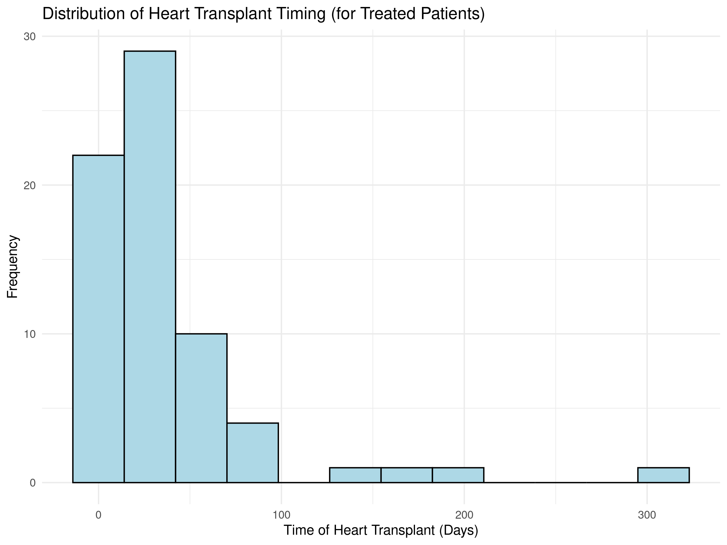
The distribution of heart transplants over time is depicted in Figure 3. This histogram illustrates the timing of transplants, highlighting any temporal trends or clustering of transplants throughout the study period. Understanding this distribution is essential for assessing time-related factors that may impact outcomes and for properly adjusting the model to account for these temporal effects.
| Variable | mean | sd | |
|---|---|---|---|
| 1 | age | 45.17 | 9.80 |
| 2 | surgery | 0.16 | 0.36 |
| 3 | year | 3.36 | 1.86 |
| 4 | trt | 0.67 | 0.47 |
6.2 Showing effect of ignoring in time-variation in treatment using HTE
In this section, we assess the impact of incorporating time-varying information on the marginal effect of treatment. Specifically, we compare two Cox proportional hazards models: one that ignores the time-varying nature of the transplant variable and treats it as a fixed covariate, and another that includes the time-varying effect by dynamically updating transplant status throughout the study.
Here we consider the same baseline regressors (age, surgery, and year), but now use them to estimate the heterogeneous treatment effects (HTE). We focus on the coefficients related to the interaction between the treatment (transplant status) and the baseline covariates to understand how the treatment effect varies across different subgroups of the population.
Table 2 shows differences between the two models. In the model ignoring treatment time, the surgery-treatment interaction shows a significant effect (, ), suggesting a transplant benefit for patients who have had previous surgery. However, this effect disappears in the model that includes treatment time (, ). The treatment variable itself also shows this difference. Other interactions remain non-significant in both models.
To summarize, ignoring time variation can lead to inflated treatment effect estimates. This occurs because ignoring time variation mistakenly treats control time as treatment time, whereas accounting for time variation correctly captures the temporal nature of treatment administration.
| Variable | Ignore Treatment Time | Include Treatment Time | ||
|---|---|---|---|---|
| Coef (SE) | P-value | Coef (SE) | P-value | |
| Trt | -1.504 (0.292) | 0.00 | 0.117 (0.340) | 0.73 |
| Age Trt | -0.259 (0.285) | 0.36 | 0.286 (0.254) | 0.26 |
| Surgery Trt | -2.191 (0.778) | 0.00 | -0.557 (0.777) | 0.47 |
| Year Trt | 0.206 (0.261) | 0.43 | 0.421 (0.260) | 0.11 |
6.3 Effects of Machine Learning and Time-Varying Causal Survival Learning
After demonstrating the effect of ignoring time-variation in treatment, we now focus on including time-variation and comparing an outcome-based method (S-lasso) to a cross-fit, doubly robust method (TV-CSL).
To do this, we first estimate and from the original dataset using TV-CSL and use these estimates as ground truth. To achieve reliable estimates, we exclude the binary variable surgery because it has a true-to-false ratio of 76% (82 of 108). During cross-fitting, this variable could result in even more extreme ratios, hence leading to unreliable estimates. We also use a linear model for because, as observed in simulations, simpler models are preferable with small sample sizes (the sample size here is 108) to avoid issues with cross-fitting.
We then design a linear treatment model and sample the treatment times. Note that these treatment times represent the waiting period after a patient enters the registry and is primarily matched by blood type (though blood type data is unavailable). Age should not be a dependent factor, but years of admission could impact treatment time to model donor availability. Therefore, we use a univariate linear model: .
We repeat the sampling-estimation procedure 100 times. The comparison is based on the average mean squared difference between the estimated effect and the ”true” effect.
| Baseline Outcome Model | ||
|---|---|---|
| Method | complex | linear |
| S-lasso | 0.386 | 0.492 |
| TV-CSL | 1.220 | 1.150 |
Table 3 presents the mean squared error (MSE) comparison between different methodological approaches. We have the following findings: First, TV-CSL performs worse than the single-fit method across both baseline models. This aligns with our simulation findings regarding small sample performance. Second, when using single S-lasso, the complex baseline outcome model shows modest improvement over its linear counterpart, with MSEs of 0.386 and 0.492 respectively.
7 Conclusion
In this paper, we propose a novel framework for estimating causal effects of time-varying treatments on time-to-event outcomes by extending the staggered adoption framework from econometrics to a survival analysis setting. Our approach leverages the Cox proportional hazards model and incorporates double machine learning (DML) to address complexities in real-world data, such as nonlinear covariate relationships and high-dimensional settings. Through simulations, we demonstrate that our estimator effectively reduces bias and improves efficiency compared to traditional outcome-based methods.
The implications of this work extend beyond healthcare to domains with time-dependent outcomes and random intervention timing. In healthcare, our method enables better understanding of how interventions like organ transplants affect patient survival based on individual characteristics, helping improve patient selection and timing of procedures. In business settings, particularly subscription-based services, our framework enables more accurate estimation of how interventions like free trials causally affect time-to-conversion outcomes. By accounting for both intervention timing and unit characteristics while maintaining methodological rigor, our approach provides reliable insights for optimizing customer acquisition and retention strategies across industries.
Our proposed estimator advances the capabilities of causal inference in survival analysis, providing a robust approach for analyzing staggered treatment adoption with time-varying interventions in diverse applied contexts.
7.1 Limitations and Future Work
Our study has several limitations that warrant discussion. A key limitation is our assumption of linear treatment effect heterogeneity. Although this specification allows substantial methodological progress and provides interpretable results for medical decision-making, treatment effects in complex medical interventions may exhibit non-linear patterns across patient characteristics. Future work could extend our framework to accommodate more flexible specifications of using non-parametric or semi-parametric approaches.
Another limitation is that in reality, there is an instantaneous increase in risk immediately after heart transplant. This occurs because some patients may experience severe rejection reactions when receiving a new heart (Lipkova et al., 2022). After surviving this critical period, the patient’s risk typically decreases. In future work, rather than modeling a single hazard function post-transplant as we did, we should consider two distinct hazard functions: one capturing the elevated risk immediately after transplant, and another reflecting the lower risk level that follows successful adaptation.
Another promising direction is to develop testing procedures for identifying which patients benefit most from transplantation, building upon our effect estimation framework. While Dukes et al. (2024) established testing procedures for continuous outcomes, similar methodologies could be developed for time-to-event outcomes.
References
- Abbring (2008) Jaap H Abbring. The event-history approach to program evaluation. In Modelling and Evaluating Treatment Effects in Econometrics, pages 33–55. Emerald Group Publishing Limited, 2008.
- Abbring and Van den Berg (2005) Jaap H Abbring and Gerard J Van den Berg. Social experiments and instrumental variables with duration outcomes. 2005.
- Akintoye et al. (2020) Emmanuel Akintoye, Doosup Shin, Paulino Alvarez, and Alexandros Briasoulis. State-level variation in waitlist mortality and transplant outcomes among patients listed for heart transplantation in the us from 2011 to 2016. JAMA network open, 3(12):e2028459–e2028459, 2020.
- Almathami et al. (2024) Hassan Khader Y Almathami, Khin Than Win, and Elena Vlahu-Gjorgievska. Empirical evidence of internal and external factors influencing users’ motivation toward teleconsultation use. Telemedicine and e-Health, 30(1):141–156, 2024.
- Almond et al. (2009) Christopher SD Almond, Ravi R Thiagarajan, Gary E Piercey, Kimberlee Gauvreau, Elizabeth D Blume, Heather J Bastardi, Francis Fynn-Thompson, and TP Singh. Waiting list mortality among children listed for heart transplantation in the united states. Circulation, 119(5):717–727, 2009.
- Andersen et al. (1993) Per Kragh Andersen, Ørnulf Borgan, Richard D. Gill, and Niels Keiding. Statistical Models Based on Counting Processes. Springer Series in Statistics. Springer US, New York, NY, 1993. ISBN 978-0-387-94519-4, 978-1-4612-4348-9. 10.1007/978-1-4612-4348-9. URL http://link.springer.com/10.1007/978-1-4612-4348-9.
- Athey and Imbens (2022) Susan Athey and Guido W Imbens. Design-based analysis in difference-in-differences settings with staggered adoption. Journal of Econometrics, 226(1):62–79, 2022.
- Cascino et al. (2022) Thomas M. Cascino, Jeffrey S. McCullough, Xiaoting Wu, Michael J. Pienta, James W. Stewart, Robert B. Hawkins, Alexander A. Brescia, Ashraf Abou El Ala, Min Zhang, Pierre-Emmanuel Noly, Jonathan W. Haft, Jennifer A. Cowger, Monica Colvin, Keith D. Aaronson, Francis D. Pagani, Donald S. Likosky, Michigan Congestive Heart Failure Investigators, Khalil M Nassar, Paul Tang, Grace Chung, Tessa Watt, Michael P Thompson, and Allison M Janda. Comparison of Evaluations for Heart Transplant Before Durable Left Ventricular Assist Device and Subsequent Receipt of Transplant at Transplant vs Nontransplant Centers. JAMA Network Open, 5(11):e2240646, November 2022. ISSN 2574-3805. 10.1001/jamanetworkopen.2022.40646. URL https://jamanetwork.com/journals/jamanetworkopen/fullarticle/2798133.
- Chernozhukov et al. (2018) Victor Chernozhukov, Denis Chetverikov, Mert Demirer, Esther Duflo, Christian Hansen, Whitney Newey, and James Robins. Double/debiased machine learning for treatment and structural parameters, 2018.
- Choudhry et al. (2019) Swati Choudhry, Yunfei Wang, Susan W Denfield, Antonio G Cabrera, Jack F Price, Hari P Tunuguntla, Vikas R Dharnidharka, Charles E Canter, and William J Dreyer. A recipient risk prediction tool for short-term mortality after pediatric heart transplantation. Transplantation, 103(11):2434–2439, 2019.
- Cox (1972) David R Cox. Regression models and life-tables. Journal of the Royal Statistical Society: Series B (Methodological), 34(2):187–202, 1972.
- Crowley and Hu (1977) John Crowley and Marie Hu. Covariance analysis of heart transplant survival data. Journal of the American Statistical Association, 72(357):27–36, 1977.
- Cui et al. (2023) Yifan Cui, Michael R Kosorok, Erik Sverdrup, Stefan Wager, and Ruoqing Zhu. Estimating heterogeneous treatment effects with right-censored data via causal survival forests. Journal of the Royal Statistical Society Series B: Statistical Methodology, 85(2):179–211, 2023.
- DeFilippis et al. (2022) Ersilia M DeFilippis, Kiran K Khush, Maryjane A Farr, Amy Fiedler, Arman Kilic, and Michael M Givertz. Evolving characteristics of heart transplantation donors and recipients: Jacc focus seminar. Journal of the American College of Cardiology, 79(11):1108–1123, 2022.
- Dukes et al. (2024) Oliver Dukes, Mats J Stensrud, Riccardo Brioschi, and Aaron Hudson. Nonparametric tests of treatment effect homogeneity for policy-makers. arXiv preprint arXiv:2410.00985, 2024.
- Evans et al. (1986) Roger W Evans, Diane L Manninen, Louis P Garrison, and Anthony M Maier. Donor availability as the primary determinant of the future of heart transplantation. Jama, 255(14):1892–1898, 1986.
- Fisher and Lin (1999) Lloyd D. Fisher and D. Y. Lin. Time-dependent covariates in the cox proportional-hazards regression model. Annual Review of Public Health, 20(1):145–157, May 1999. ISSN 0163-7525, 1545-2093. 10.1146/annurev.publhealth.20.1.145. URL https://www.annualreviews.org/doi/10.1146/annurev.publhealth.20.1.145.
- Fleming and Harrington (2005) Thomas R. Fleming and David P. Harrington. Counting processes and survival analysis. Wiley series in probability and statistics. Wiley-Interscience, New York, 2005. ISBN 978-0-471-76988-0.
- Foster and Syrgkanis (2023) Dylan J. Foster and Vasilis Syrgkanis. Orthogonal Statistical Learning, June 2023. URL http://arxiv.org/abs/1901.09036. arXiv:1901.09036 [cs, econ, math, stat].
- Gao and Hastie (2021) Zijun Gao and Trevor Hastie. Estimating heterogeneous treatment effects for general responses. arXiv preprint arXiv:2103.04277, 2021.
- Goodman-Bacon (2021) Andrew Goodman-Bacon. Difference-in-differences with variation in treatment timing. Journal of econometrics, 225(2):254–277, 2021.
- Gopalakrishnan and Park (2021) Arun Gopalakrishnan and Young-Hoon Park. The impact of coupons on the visit-to-purchase funnel. Marketing Science, 40(1):48–61, 2021.
- Hastie et al. (2009) Trevor Hastie, Robert Tibshirani, Jerome H Friedman, and Jerome H Friedman. The elements of statistical learning: data mining, inference, and prediction, volume 2. Springer, 2009.
- Hern’an (2010) Miguel A Hern’an. The hazards of hazard ratios. Epidemiology, 21(1):13–15, 2010.
- Imai and Kim (2021) Kosuke Imai and In Song Kim. On the use of two-way fixed effects regression models for causal inference with panel data. Political Analysis, 29(3):405–415, 2021.
- Imai and Ratkovic (2013) Kosuke Imai and Marc Ratkovic. Estimating treatment effect heterogeneity in randomized program evaluation. 2013.
- Kalbfleisch and Prentice (2011) John D Kalbfleisch and Ross L Prentice. The statistical analysis of failure time data. John Wiley & Sons, 2011.
- Kennedy (2023) Edward H. Kennedy. Towards optimal doubly robust estimation of heterogeneous causal effects, August 2023. URL http://arxiv.org/abs/2004.14497. arXiv:2004.14497 [math, stat].
- Khush et al. (2013) Kiran K. Khush, Rebecca Menza, John Nguyen, Jonathan G. Zaroff, and Benjamin A. Goldstein. Donor Predictors of Allograft Use and Recipient Outcomes After Heart Transplantation. Circulation: Heart Failure, 6(2):300–309, March 2013. ISSN 1941-3289, 1941-3297. 10.1161/CIRCHEARTFAILURE.112.000165. URL https://www.ahajournals.org/doi/10.1161/CIRCHEARTFAILURE.112.000165.
- Kilic et al. (2021) Arman Kilic, Michael A Mathier, Gavin W Hickey, Ibrahim Sultan, Victor O Morell, Suresh R Mulukutla, and Mary E Keebler. Evolving trends in adult heart transplant with the 2018 heart allocation policy change. JAMA cardiology, 6(2):159–167, 2021.
- Klein and Moeschberger (1997) John P. Klein and Melvin L. Moeschberger. Survival Analysis. Statistics for Biology and Health. Springer New York, New York, NY, 1997. ISBN 978-1-4757-2730-2 978-1-4757-2728-9. 10.1007/978-1-4757-2728-9. URL http://link.springer.com/10.1007/978-1-4757-2728-9.
- Künzel et al. (2019) Sören R. Künzel, Jasjeet S. Sekhon, Peter J. Bickel, and Bin Yu. Metalearners for estimating heterogeneous treatment effects using machine learning. Proceedings of the National Academy of Sciences, 116(10):4156–4165, March 2019. ISSN 0027-8424, 1091-6490. 10.1073/pnas.1804597116. URL https://pnas.org/doi/full/10.1073/pnas.1804597116.
- Li and Greene (2015) Lingling Li and Tom Greene. Evaluating the effect of health care interventions using doubly robust estimation. Statistics in Medicine, 34(3):539–559, 2015.
- Lipkova et al. (2022) Jana Lipkova, Tiffany Y Chen, Ming Y Lu, Richard J Chen, Maha Shady, Mane Williams, Jingwen Wang, Zahra Noor, Richard N Mitchell, Mehmet Turan, et al. Deep learning-enabled assessment of cardiac allograft rejection from endomyocardial biopsies. Nature medicine, 28(3):575–582, 2022.
- Nie and Wager (2021) Xinkun Nie and Stefan Wager. Quasi-oracle estimation of heterogeneous treatment effects. Biometrika, 108(2):299–319, 2021.
- Nie et al. (2021) Xinkun Nie, Emma Brunskill, and Stefan Wager. Learning when-to-treat policies. Journal of the American Statistical Association, 116(533):392–409, 2021.
- O’Connell et al. (1992) John B O’Connell, Robert C Bourge, Maria Rosa Costanzo-Nordin, David J Driscoll, James P Morgan, EA Rose, and BF Uretsky. Cardiac transplantation: recipient selection, donor procurement, and medical follow-up. a statement for health professionals from the committee on cardiac transplantation of the council on clinical cardiology, american heart association. Circulation, 86(3):1061–1079, 1992.
- Parker et al. (2019) William F. Parker, Allen S. Anderson, Robert D. Gibbons, Edward R. Garrity, Lainie F. Ross, Elbert S. Huang, and Matthew M. Churpek. Association of Transplant Center With Survival Benefit Among Adults Undergoing Heart Transplant in the United States. JAMA, 322(18):1789, November 2019. ISSN 0098-7484. 10.1001/jama.2019.15686. URL https://jamanetwork.com/journals/jama/fullarticle/2754791.
- Power et al. (2024) Alyssa Power, Kurt R. Sweat, Alvin Roth, John C. Dykes, Beth Kaufman, Michael Ma, Sharon Chen, Seth A. Hollander, Elizabeth Profita, David N. Rosenthal, Lynsey Barkoff, Chiu-Yu Chen, Ryan R. Davies, and Christopher S. Almond. Contemporary Pediatric Heart Transplant Waitlist Mortality. Journal of the American College of Cardiology, 84(7):620–632, August 2024. ISSN 07351097. 10.1016/j.jacc.2024.05.049. URL https://linkinghub.elsevier.com/retrieve/pii/S0735109724075624.
- Robins et al. (1992) James M Robins, Andrea Rotnitzky, and Lue Ping Zhao. Estimation of regression coefficients when some regressors are not always observed. Journal of the American Statistical Association, 87(420):1013–1022, 1992.
- Rubin (1974) Donald B Rubin. Estimating causal effects of treatments in randomized and nonrandomized studies. Journal of educational Psychology, 66(5):688, 1974.
- Shaikh and Toulis (2021) Azeem M Shaikh and Panos Toulis. Randomization tests in observational studies with staggered adoption of treatment. Journal of the American Statistical Association, 116(536):1835–1848, 2021.
- Sun and Abraham (2021) Liyang Sun and Sarah Abraham. Estimating dynamic treatment effects in event studies with heterogeneous treatment effects. Journal of econometrics, 225(2):175–199, 2021.
- Tay et al. (2023) J. Kenneth Tay, Balasubramanian Narasimhan, and Trevor Hastie. Elastic Net Regularization Paths for All Generalized Linear Models. Journal of Statistical Software, 106(1):1–31, 2023. 10.18637/jss.v106.i01. URL https://www.jstatsoft.org/index.php/jss/article/view/v106i01.
- Trulock et al. (2007) Elbert P Trulock, Jason D Christie, Leah B Edwards, Mark M Boucek, Paul Aurora, David O Taylor, Fabienne Dobbels, Axel O Rahmel, Berkeley M Keck, and Marshall I Hertz. Registry of the international society for heart and lung transplantation: twenty-fourth official adult lung and heart–lung transplantation report—2007. The Journal of heart and lung transplantation, 26(8):782–795, 2007.
- Van der Vaart (2000) Aad W Van der Vaart. Asymptotic statistics, volume 3. Cambridge university press, 2000.
- Vansteelandt and Joffe (2014) Stijn Vansteelandt and Marshall Joffe. Structural Nested Models and G-estimation: The Partially Realized Promise. Statistical Science, 29(4), November 2014. ISSN 0883-4237. 10.1214/14-STS493. URL https://projecteuclid.org/journals/statistical-science/volume-29/issue-4/Structural-Nested-Models-and-G-estimation--The-Partially-Realized/10.1214/14-STS493.full.
- Wang et al. (2024) Yuyao Wang, Andrew Ying, and Ronghui Xu. Learning treatment effects under covariate dependent left truncation and right censoring, November 2024. URL http://arxiv.org/abs/2411.18879. arXiv:2411.18879 [stat].
- Xu et al. (2024) Shenbo Xu, Raluca Cobzaru, Stan N. Finkelstein, Roy E. Welsch, Kenney Ng, and Zach Shahn. Estimating Heterogeneous Treatment Effects on Survival Outcomes Using Counterfactual Censoring Unbiased Transformations, September 2024. URL http://arxiv.org/abs/2401.11263. arXiv:2401.11263 [stat].
- Xu et al. (2022) Yizhe Xu, Nikolaos Ignatiadis, Erik Sverdrup, Scott Fleming, Stefan Wager, and Nigam Shah. Treatment Heterogeneity for Survival Outcomes, September 2022. URL http://arxiv.org/abs/2207.07758. arXiv:2207.07758 [stat].
- Zhang et al. (2017) Ping Zhang, Fei Wang, Jianying Hu, and Robert Sorrentino. Mining electronic health records using real-world evidence for clinical research. IEEE Intelligent Systems, 32(6):50–56, 2017.
- Zhu and Gallego (2022) Jie Zhu and Blanca Gallego. Causal inference for observational longitudinal studies using deep survival models. Journal of Biomedical Informatics, 131:104119, 2022.
- Zhu et al. (2021) Yuanjia Zhu, Bharathi Lingala, Michael Baiocchi, Veronica Toro Arana, Kiah M Williams, Yasuhiro Shudo, Philip E Oyer, and Y Joseph Woo. The stanford experience of heart transplantation over five decades. European Heart Journal, 42(48):4934–4943, 2021.
Appendix A Derivation of the TV-CSL Estimator
The main technique involves expanding the log-likelihood of the data around the true parameter to obtain a score that approximates the true parameter at the fastest possible rate. See the next section for a derivation of the likelihood expansion. A key result from that section is the estimating equation resulting from the optimal score:
| (12) |
Use the tower property to take inside, we obtain
| (13) |
where
Note that . Taking inside, we obtain
| (14) |
Hence we need
| (15) |
Here, is the marginal censoring probability.
Hence, . When for all , i.e., when all observations are not-censored, then is the treated probability at time for a unit with covariate .
Appendix B Key Lemma for Deriving the Score Function
Here we derive the key lemma that shows how the estimator is obtained. The key step is to calculate the expansion of the likelihood. Let denote the log-likelihood of the exponential family. Lemma 1 of Gao and Hastie (2021) states that for arbitrary , the likelihood of satisfies
where .
Further
| (16) |
The key insight is that we parametrize , where . Instead of parametrizing using and , we re-parametrize it by adding and subtracting to obtain double robustness.
When comparing and , we keep and fixed, choosing and . This implies that . We can then apply this to Equation 16:
| (17) |
Move the negative sign, we have
| (18) |
We take the expectation, and maximize the LHS by differentiating , and set the derivactive to zero (this is to find the tangent direction)
| (19) |
This says
| (20) |
We also want . This is because we are taking one-dimentional efficient scores so we finally need tangency. The condition is that the numerator is zero, i.e.
| (21) |
Plugin , and taking as random variables, we have
Appendix C Proof of Proposition 1
Proof333The proof structure follows the approach of Gao and Hastie (2021), which we have independently verified for our specific context of survival analysis with random treatment timing. In subsequent versions, we will extend this foundation with additional martingale arguments that address the survival model present in our setting, further strengthening the theoretical guarantees for our estimator.: We write , where is a unit directional vector, and is the distance from to . Similarly, we can write , where . By the assumption of proposition 1, , .
The score function for the partial likelihood of the -th sample is:
where .
Denote the expected score as and define the empirical score . For simplicity, we write as
We first show is consistent under . Taylor’s expansion of at is
where .
Note that (See Fleming and Harrington (2005), Chapter 8 for a proof). Thus . We now argue where .
We make the following decomposition:
The last term in the bracket is an empirical process term. Given that our score function is a Donsker class, and is consistent, the empirical process term is (Lemma 19.24 of Van der Vaart (2000)).
Furthermore, by mean value theorem,
for some .
Thus,
| (22) |
Furthermore, by central limit theorem (CLT),
Notice that are bounded, i.e., they are both
Then, because the minimum eigenvalue of and is lower bounded, the above turns to :
Therefore, is consistent.
We now prove the rate result. To do this, we make a second order Taylor’s expansion of at :
where .
The first order Taylor’s expansion of at is:
where we apply the CLT in the second equation and use in the last equation due to the Neyman orthogonality of the score function for the partial likelihood (see Appendix in Gao and Hastie (2021) for a proof). A similar analysis holds for .
Combining these results:
where we use the boundedness of the second derivatives. Since the minimal eigenvalue of is uniformly lower bounded by , we have:
This completes the proof.
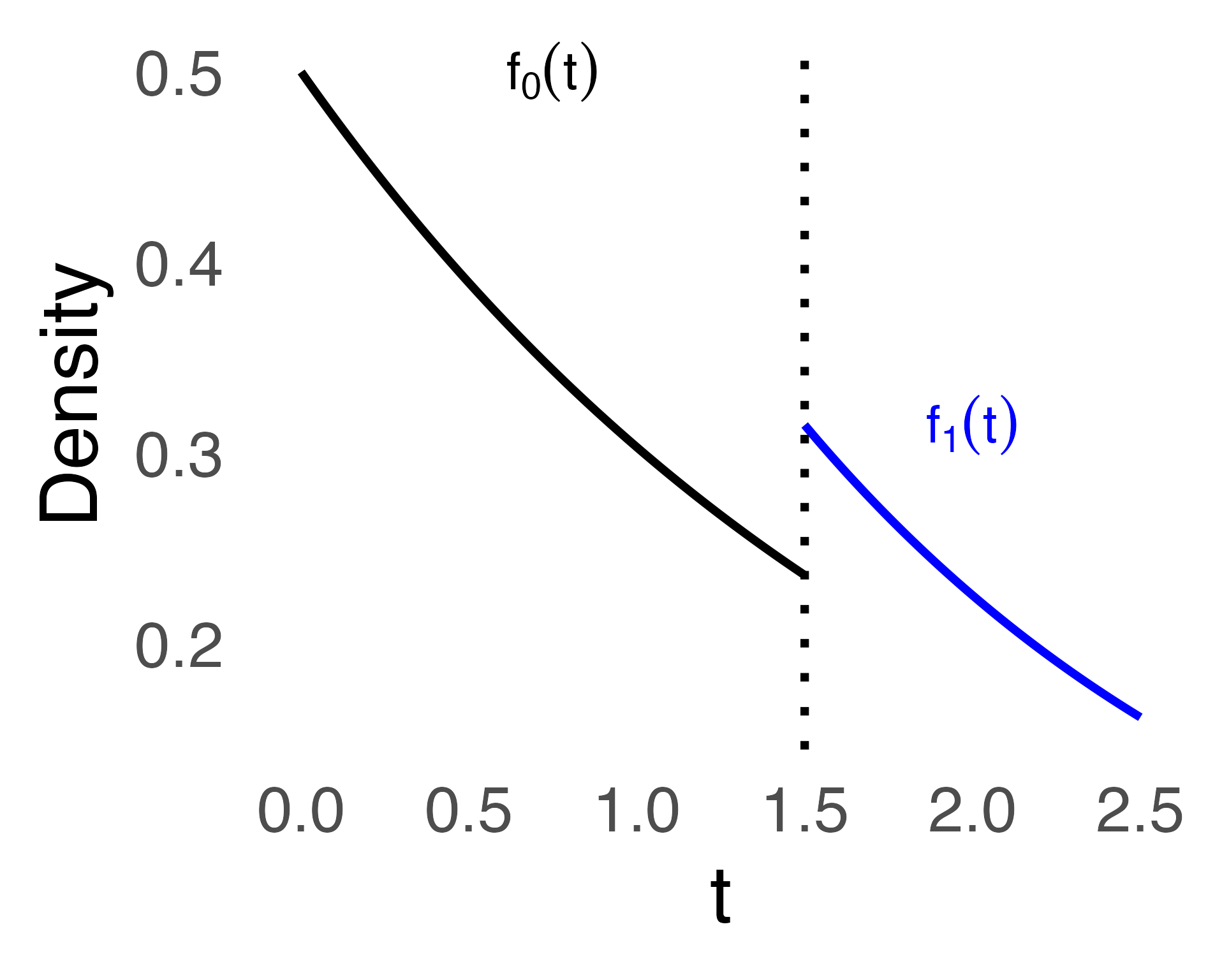
Appendix D Parametrizing the PDF for the Piecewise Cox Model
Given two probability density functions (PDFs) and , there are two ways to parametrize the desired piecewise PDF to show treatment effect. Both parametrizations integrate to one and are illustrated in Figure 4.
Parametrization 1:
| (23) |
Parametrization 2:
| (24) |
Question:
Are these parametrizations equivalent? If not, which one is preferable?
Answer:
No, they are not equivalent in general. Let’s convert Parametrizations 1 and 2 into hazard functions. We only need to compare the expressions for . For clarity of notation, we omit the conditioning on in the derivations below.
Parametrization 1:
For :
The denominator:
Therefore:
Parametrization 2:
For :
The denominator:
Therefore:
Discussion
Parametrization 1 yields , while Parametrization 2 yields . These are equivalent only when is constant. For example, if , the parametrizations differ. Therefore, the equivalence PDF parametrization from the paper’s hazard model corresponds to Parametrization 1.