Quantile Residual Lifetime Regression for Multivariate Failure Time Data

Abstract

The quantile residual lifetime (QRL) regression is an attractive tool for assessing covariate effects on the distribution of residual life expectancy, which is often of interest in clinical studies. When the study subjects are exposed to multiple events of interest, the failure times observed for the same subject are potentially correlated. To address such correlation in assessing the covariate effects on QRL, we propose a marginal semiparametric QRL regression model for multivariate failure time data. Our new proposal facilitates estimation of the model parameters using unbiased estimating equations and results in estimators, which are shown to be consistent and asymptotically normal. To overcome additional challenges in inference, we provide three methods for variance estimation based on resampling techniques and a sandwich estimator, and further develop a Wald-type test statistic for inference. The simulation studies and a real data analysis offer evidence of the satisfactory performance of the proposed method.

Key words: Multivariate failure times; quantile residual lifetime; inverse probability of censoring weighting; perturbation resampling; sandwich estimator.

1 Introduction

Multivariate failure times arise frequently in biomedical research due to study subjects’ exposure to multiple types of failure events, recurrence of the same event type in longitudinal studies, or subjects being nested within clusters. This clustering may arise from various scenarios, including recurrence of the same event type in longitudinal studies, or the same event type occurring in clustered organs on the same subject such as the time to blindness of the two eyes (Diabetic Retinopathy Study Research Group,, 1976) and tooth extraction times (Caplan et al.,, 2005) on the same subject. Failure times of interest obtained from the same cluster exhibit inherent association, which needs to be accounted for in the analysis of such data.

Studying the distribution of residual lifetime generally provides valuable insights into disease prevention or treatment strategies for individuals at different life stages, especially for those who may not be at short-term risk of disease (Conner et al.,, 2022). In the Framingham heart study (Tsao and Vasan,, 2015), each study subject may experience several cardiovascular diseases (events), such as coronary heart disease, myocardial infarction and hypertension, and potential dependence arises among the multiple disease event times obtained from a subject (cluster). It is interesting in this study to assess the effects of risk factors, e.g., BMI, blood pressure, cholesterol level, smoking and gender, on the distribution of remaining life times to the occurrence of each disease given that a subject is known to be disease-free at some followup time point. Since the dependence structure among multiple residual life times of a subject is unknown in practice, it poses both theoretical and computational challenges in regression analysis.

Classical methods of handling correlated failure times can be basically divided into three classes. The first class explicitly models the dependence among multivariate failure times within a subject/cluster through frailty, which is often assumed to follow a known distribution from some positive scale family (Aalen,, 1988; Duchateau and Janssen,, 2008). The second class employs a copula function to model the underlying association within the same cluster (Othus and Li,, 2010; Kwon et al.,, 2022; He et al.,, 2024). The third class consists of marginal models, initially proposed by Liang and Zeger, (1986) for longitudinal outcomes. The marginal model approach has been widely adopted and remains an active area of research. In particular, it has been extensively studied in the context of multivariate survival data under the Cox proportional hazards or AFT models (e.g. Cai and Prentice,, 1995; Jin et al.,, 2006; Chen et al.,, 2010; Lin,, 2014; Xu et al.,, 2023) and censored quantile regression (Yin and Cai,, 2005; Wang and Fygenson,, 2009). The basic idea of marginal models is model the marginal distributions of multivariate outcomes as for independent observations, and treats associations among outcomes as a nuisance. Without specifying the correlation structure, this approach allows for more flexible, parsimonious models and is computationally more efficient than frailty or copula-based models.

Our work in this paper focuses on the marginal method for regression analysis of multivariate residual lifetimes. As an alternative to the aforementioned marginal models, regression analysis based on residual lifetimes has attracted considerable interests in clinical studies due to its ease of understanding and capability to align with the demands in practice. For example, in cancer studies with patients who survived after some initial treatments, their remaining lifetimes are often of interest in evaluating the efficacy of the followup therapies. Compared to relative risks, the remaining life expectancy is more straightforward and readily understandable for patients. Recently, the frailty model was extended to regression analysis of mean residual lifetimes in multicenter studies by Huang et al., (2019) using a hierarchical likelihood approach. It is noted that failure times in biomedical studies often exhibit censorship, outliers and heteroscedasticity, which particularly leads to covariate effects on the remaining lifetimes varying over different follow-up stages. To this end, quantile regression appears more appropriate than the mean-based regression for the remaining lifetimes.

The quantile residual lifetime (QRL) regression, which leverages the strengths of censored quantile regression (Peng and Huang,, 2008; Wang and Wang,, 2009), investigates the relationship between the quantile residual lifetimes and a set of covariates, and it has gained increased attention recently. A review of early developments of the QRL models can be found in the monograph by Jeong, (2014). Jeong et al., (2008) proposed nonparametric estimation for the median residual lifetimes. Semiparametric QRL regression analysis has been investigated for univariate failure time outcomes. Jung et al., (2009) extended Ying et al., (1995)’s median regression model to quantile residual lifetimes and mimicked the least square estimating equations to construct an estimating equation for quantile coefficients. They suggested a grid search method to find some appropriate roots, which is computationally expensive especially in the presence of a large number of covariates because the estimating equation is neither monotone nor continuous. For testing significance, they studied a score-type test. Zhou and Jeong, (2011) and Kim et al., (2012) proposed case-weighted empirical-likelihood ratio test. Built upon Jung et al., (2009)’s method, Ma and Wei, (2012) estimated quantile coefficient by spline smoothing instead and suggested a Wald-type test statistic. For data with longitudinal covariates, Li et al., (2016) and Lin et al., (2019) developed an unbiased estimating equation that is solved via linear programming. All these existing inferential methods for QRL models are under the independence assumption for failure times.

In the presence of multivariate or clustered failure times, applying these methods by ignoring possible correlations among outcome data may result in biases in variance estimation and loss of statistical power for testing hypotheses in consequence. To circumvent this issue, we study a marginal QRL regression model for multivariate failure time data, extending the idea of QRL regression Li et al., (2016) to accommodate the correlation among multiple failure time outcomes of a subject. We develop semiparametric estimating equations for parameter estimation and show theoretical properties of the resulting estimator regardless of the true dependence structures. A major hurdle in inference for QRL regression is variance estimation of parameter estimators. To this end, we propose three methods to estimate the covariance matrix of the estimated regression coefficients accounting for the dependence of the multivariate failure times properly and compare their performance numerically.

The rest of this article is organized as follows. In Section 2, we introduce notation for data and the proposed marginal QRL regression model first, and then provide the estimating equations for model parameters. In Section 3, we establish asymptotic properties of the resulting estimator and provide methods for variance estimation for inference. The performance of the proposed estimators is examined through extensive simulation studies in Section 4. We present an application to the analysis of the Flamingham Heart data in Section 5, followed by concluding remarks in Section 6.

2 Methodology

2.1 Data and marginal QRL regression model

Consider a sample comprising $n$ clusters with each cluster containing $m_{i}$ observations. Consequently, the total number of observations in the sample amounts to $N=\sum_{i=1}^{n}m_{i}$. Let $T_{ij}$ represent the $j$-th event time of cluster $i$ for $j=1,\ldots,m_{i}$ and $i=1,\ldots,n$ and $\mathbf{X}_{ij}$ be the associated baseline covariate vector with the first element being one. At a specific time point $t_{0}$, we define $\theta_{\tau,t_{0}}$ as the $\tau$-th conditional quantile of the residual lifetime on a logarithmic scale, i.e., $\log(T_{ij}-t_{0})$, conditional on the covariates $\mathbf{X}_{ij}$ and subject to the constraint $T_{ij}>t_{0}$. As a result, $\theta_{\tau,t_{0}}$ satisfies the equation $\operatorname{Pr}(\log(T_{ij}-t_{0})\leq\theta_{\tau,t_{0}}|T_{ij}\geq t_{0},\mathbf{X}_{ij})=\tau$, which is equivalent to

$$\operatorname{Pr}(t_{0}\leq T_{ij}\leq t_{0}+\exp(\theta_{\tau,t_{0}})|\mathbf{X}_{ij})=\tau\operatorname{Pr}(T_{ij}\geq t_{0}|\mathbf{X}_{ij}).$$ (1)

For the $\tau$-th quantile of the remaining lifetimes among clusters whose event times are beyond time $t_{0}$, the linear QRL regression is assumed in the form of

$$\theta_{\tau,t_{0}}=\mathbf{X}_{ij}^{T}\bm{\alpha}_{\tau,t_{0}},$$ (2)

where $\bm{\alpha}_{\tau,t_{0}}$ is the vector of coefficients at time $t_{0}$ for covariate vector $\mathbf{X}_{ij}$ at some quantile level $\tau\in(0,1)$. Under model (2), $T_{ij}$ can be modeled as

$$\log(T_{ij}-t_{0})=\mathbf{X}_{ij}^{T}\bm{\alpha}_{\tau,t_{0}}+{\color[rgb]{0,0,0}e_{ij}^{\tau}},{\color[rgb]{0,0,0}j=1,\cdots,m_{i};i=1,\cdots,n}$$ (3)

where ${\color[rgb]{0,0,0}e_{ij}^{\tau}}$’s are correlated within the same cluster but independent across clusters. For the sake of identifiability, we set the conditional $\tau$th quantile of ${\color[rgb]{0,0,0}e_{ij}^{\tau}}$ to zero given $\mathbf{X}_{ij}$ and $T_{ij}>t_{0}$.

2.2 Estimation procedure

For ease of presentation, we omit $\tau$ and $t_{0}$ in the coefficient vector $\bm{\alpha}$ in the following. When all survival times are exactly observed, the estimator of $\bm{\alpha}$ can be obtained by solving the following estimating equations for $\bm{\alpha}$:

$$\sum\limits_{i}\sum\limits_{j}\mathbf{X}_{ij}I(T_{ij}\geq t_{0})[I\{T_{ij}\leq t_{0}+\exp(\mathbf{X}_{ij}^{T}\bm{\alpha})\}-\tau]=0.$$ (4)

In the presence of right censoring, the survival outcome $T_{ij}$ is observed as $Y_{ij}=\min(T_{ij},C_{ij})$ along with the censoring indicator ${\color[rgb]{0,0,0}\Delta_{ij}}=I(T_{ij}\leq C_{ij})$, and $C_{ij}$ is the corresponding censoring time. It is assumed that $T_{ij}$ and $C_{ij}$ are conditionally independent given $\mathbf{X}_{ij}$, and $C_{ij}$ independently follows a distribution with the survival function $G(\cdot)$, which is independent from $\mathbf{X}_{ij}$. With right-censored multivariate failure time data, one may modify equations in (4) by adjusting censoring. Let $\bm{\alpha}_{0}$ be the true value of $\bm{\alpha}$. Note that

$$\begin{split}&E\left[\frac{{\color[rgb]{0,0,0}\Delta_{ij}}}{G(Y_{ij})}I\{Y_{ij}\leq t_{0}+\exp(\mathbf{X}_{ij}^{T}\bm{\alpha}_{0})\}\Bigg{|}Y_{ij}\geq t_{0},\mathbf{X}_{ij}\right]\\ &=\frac{\operatorname{Pr}\left\{t_{0}\leq T_{ij}=Y_{ij}\leq C_{ij},T_{ij}\leq t_{0}+\exp(\mathbf{X}_{ij}^{T}\bm{\alpha}_{0})\Bigg{|}\mathbf{X}_{ij}\right\}}{G(Y_{ij})\operatorname{Pr}\left\{Y_{ij}\geq t_{0}|\mathbf{X}_{ij}\right\}}\\ &=\frac{\operatorname{Pr}\left\{t_{0}\leq T_{ij}\leq t_{0}+\exp(\mathbf{X}_{ij}^{T}\bm{\alpha}_{0})|\mathbf{X}_{ij}\right\}}{\operatorname{Pr}\left\{T_{ij}\geq t_{0}|\mathbf{X}_{ij}\right\}G(t_{0})}=\frac{\tau}{G(t_{0})}.\end{split}$$ (5)

This motivates us to form a modified estimating equation for $\bm{\alpha}$ as

$$S_{N}(\bm{\alpha})=\frac{1}{N}\sum\limits_{i}\sum\limits_{j}\mathbf{X}_{ij}I(Y_{ij}\geq t_{0})\left[\frac{{\color[rgb]{0,0,0}\Delta_{ij}}I\left\{Y_{ij}\leq t_{0}+\exp(\mathbf{X}_{ij}^{T}\bm{\alpha})\right\}}{\widehat{G}(Y_{ij})/\widehat{G}(t_{0})}-\tau\right]=0,$$ (6)

where $\widehat{G}(\cdot)$ is the Kaplan-Meier estimator of $G$ based on observations $\{Y_{ij},1-{\color[rgb]{0,0,0}\Delta_{ij}}\}$. The estimating equation (6) can be viewed as a multivariate version of Li et al., (2016)’s method, designed to account for the correlation among multivariate time-to-event data. In the independent cases with time-independent covariates, $S_{N}(\bm{\alpha})$ in (6) reduces to the estimating function used in Li et al., (2016). The estimator for $\bm{\alpha}$, denoted by $\widehat{\bm{\alpha}}$, can be obtained as the solution to the estimating equations in (6). Equivalently, it is the minimizer of the following linear programming problem:

$$\begin{split}\frac{1}{N}\sum\limits_{i}\sum\limits_{j}&\frac{I(Y_{ij}\geq t_{0}){\color[rgb]{0,0,0}\Delta_{ij}}}{\widehat{G}(Y_{ij})/\widehat{G}(t_{0})}\rho_{\tau}\left\{\log(Y_{ij}-t_{0})-\mathbf{X}_{ij}^{T}\bm{\alpha}\right\}\\ &+I(Y_{ij}\geq t_{0})\rho_{\tau}\left\{A-\mathbf{X}_{ij}^{T}\bm{\alpha}\left[1-\frac{{\color[rgb]{0,0,0}\Delta_{ij}}}{\widehat{G}(Y_{ij})/\widehat{G}(t_{0})}\right]\right\},\end{split}$$ (7)

where $\rho_{\tau}(u)=u[\tau-I(u<0)]$ is the quantile loss function, and $A$ is a constant chosen to be exceptionally large such that $A>\max\limits_{i,j}\{\log(Y_{ij}-t_{0})\}$. We adopt the fast interior point algorithm (Portnoy and Koenker,, 1997) to solve this linear programming problem, which can be readily implemented via function rq() in R library quantreg using the weighted QR model on the augmented data set comprising of pseudo responses $\{(\log(Y_{11}-t_{0}),\cdots,\log(Y_{nm_{n}}-t_{0}),A,\cdots,A\}$ with corresponding covariates $\{\mathbf{X}_{11},\cdots,\mathbf{X}_{nm_{n}},\mathbf{X}_{11}^{*},\cdots,\cdots,\mathbf{X}_{nm_{n}}^{*}\}$ with $\mathbf{X}_{ij}^{*}=\left[1-{\color[rgb]{0,0,0}\Delta_{ij}}\widehat{G}(t_{0})/\widehat{G}(Y_{ij})\right]\mathbf{X}_{ij}$. An alternative optimization algorithm analogue to Li and Peng, (2015) may be considered, in which all artificial observations $\{\mathbf{X}_{ij}^{*}\}_{i,j}$ are treated as a whole unit. In some cases, these two competing optimization algorithms have negligible differences in parameter estimation when there is enough number of exactly observed residual lifetimes. For our motivating data, the optimization (7) produces much more reasonable results compared to results from a classical censored quantile regression (that is, $t_{0}=0$). This may be because Li and Peng, (2015)’s method requires a large enough constant $A$ to bound the unified value $\sum\limits_{i}\sum\limits_{j}\left[1-\frac{{\color[rgb]{0,0,0}\Delta_{ij}}}{\widehat{G}(Y_{ij})/\widehat{G}(t_{0})}\right]I(Y_{ij}\geq t_{0})\mathbf{X}_{ij}^{T}\bm{\alpha}$ for any $\bm{\alpha}$ in the parameter space, possibly leading to unstable estimation procedure especially when the magnitude of $\bm{\alpha}$ or sample size is large.

Remark 1.

Once obtaining $\widehat{\bm{\alpha}}$, the $\tau$-th conditional quantile of the logarithm of the residual lifetime for a specific individual with covariates $\mathbf{x}$ can be estimated as $\widehat{\theta}_{\tau,t_{0}}=\mathbf{x}^{T}\widehat{\bm{\alpha}}_{\tau,t_{0}}$. In practice, the estimated conditional quantiles $\widehat{\theta}_{\tau,t_{0}}$ may not be monotonically increasing in $\tau$ due to lack of sufficient data and/or quantile crossing. To account for the nonmonotonicity problem, one may follow the rearrangement method developed by Chernozhukov et al., (2010) to construct monotone quantile curves by using the order statistics of the rearranged quantile estimates. The rearrangement procedure has been commonly used in various quantile regression models (Wang et al.,, 2012; Wang and Li,, 2013; Yu et al.,, 2021). Given asymptotic properties of $\widehat{\bm{\alpha}}$ and the Wald-type inference discussed in Section 3, the confidence intervals for $\widehat{\theta}_{\tau,t_{0}}$ can be subsequently constructed. As shown by Chernozhukov et al., (2010) and Wang et al., (2012) either theoretically or numerically, the quantile estimators with/without rearrangement exhibited nearly identical performance in estimation and inference.

3 Asymptotic Properties and Inference

3.1 Consistency and asymptotic normality

The following conditions are necessary to derive the asymptotic properties of the proposed estimator obtained from solving the estimating equation in (6). To associate with the total sample size $N$, in this section, we rewrite $\widehat{\bm{\alpha}}$ as $\widehat{\bm{\alpha}}_{N}$.

Condition 1.

The parameter space for $\bm{\alpha}$, say $\mathcal{D}$, is a compact region with $\bm{\alpha}_{0}$ in the interior. For any $\bm{\alpha}\in\mathcal{D}$, suppose that there exists $t_{u}$ such that $\operatorname{Pr}\left\{\log(Y_{ij}-t_{0})\geq t_{u})|\mathbf{X}_{ij}\right\}$ is uniformly bounded away from zero and $\mathbf{X}_{ij}^{T}\bm{\alpha}\leq t_{u}$ with probability one.

Condition 2.

The estimator $\widehat{G}$ has $\sup\limits_{t\leq t_{u}}|\widehat{G}(t)-G(t)|=o(N^{-1/2+\epsilon})$ for any $\epsilon>0$.

Condition 3.

Given $T_{ij}>t_{0}$, the conditional distribution functions $F_{e}(e|\mathbf{X}_{ij})=\operatorname{Pr}({\color[rgb]{0,0,0}e_{ij}^{\tau}}\leq e|\mathbf{X}_{ij})$ have densities $f_{e}(\cdot|\mathbf{X}_{ij})$ which is Lipschitz continuous in the neighborhood of 0. We assume that $N^{-1}\sum_{ij}\operatorname{Pr}(T_{ij}\geq t_{0}|\mathbf{X}_{ij})f_{e}(0|\mathbf{X}_{ij})\mathbf{X}_{ij}\mathbf{X}_{ij}^{T}$ converges almost surely to a positive definite and bounded matrix, denoted by $\Lambda$.

Condition 4.

1) The cluster size $m_{i}$ is finite. 2) $\mathbf{X}_{ij}$ are uniformly bounded for $j=1,\cdots,m_{i}$ and $i=1,\cdots,n$.

Condition 1 is an standard condition for quantile residual lifetime regression and commonly imposed in literature (Jung et al.,, 2009). Condition 2 holds in most cases when $\hat{G}$ is the Kaplan-Meier estimator (Csörgő and Horváth,, 1983). Condition 3 is to ensure $\inf\limits_{\bm{\alpha}:||\bm{\alpha}-\bm{\alpha}_{0}||=\epsilon}||\overline{S}_{N}(\bm{\alpha})||>0$ for any $\epsilon>0$, which is needed to establish consistency of the estimator $\widehat{\bm{\alpha}}_{N}$. Matrix $\Lambda$, defined in Condition 3, will be part of the slope matrix in estimator’ asymptotic variance, and its positive definiteness and boundness guarantee the asymptotic normality of the estimator $\widehat{\bm{\alpha}}_{N}$. Condition 4 is a weak assumption and commonly seen in literature.

To justify the asymptotic properties of the proposed estimator, we consider the conditional expectation of the proposed estimating function (6) with substitution of true censoring distribution and define

$$\overline{S}_{N}(\bm{\alpha})=\frac{1}{N}\sum\limits_{i}\sum\limits_{j}\mathbf{X}_{ij}G(t_{0})\left[\operatorname{Pr}\left\{t_{0}\leq T_{ij}\leq t_{0}+\exp(\mathbf{X}_{ij}^{T}\bm{\alpha})|\mathbf{X}_{ij}\right\}-\tau\operatorname{Pr}\left\{T_{ij}\geq t_{0}|\mathbf{X}_{ij}\right\}\right].$$ (8)

By the definition of quantile residual lifetime function in equation (1), it follows that $\bm{\alpha}_{0}$ is the unique root of $\overline{S}_{N}(\bm{\alpha})=0$ for some commonly used distributions of the failure time $T$, provided that its survival function is continuous and strictly decreasing with a closed form (Jeong,, 2014).

Theorem 1.

(Consistency.) Under Conditions 1-3, $\widehat{\bm{\alpha}}_{N}$ satisfying $S_{N}(\widehat{\bm{\alpha}}_{N})=o(1)$ converges almost surely to $\bm{\alpha}_{0}$ as $N\rightarrow\infty$.

Lemma 1.

If Condition 1 holds, $N^{1/2}S_{N}(\bm{\alpha}_{0})$ converges to a zero-mean normal distribution with the asymptotic covariance matrix $\Sigma$ as defined in the proof of this lemma in the Appendix.

Theorem 2.

(Asymptotic normality.) Under Conditions 1- 4, $\widehat{\bm{\alpha}}_{N}$ satisfying $S_{N}(\widehat{\bm{\alpha}}_{N})=o(N^{-1/2})$ is asymptotically normal, i.e., $N^{1/2}(\widehat{\bm{\alpha}}_{N}-\bm{\alpha}_{0})\xrightarrow{d}N(0,V(\bm{\alpha}_{0}))$, where $V(\bm{\alpha}_{0})=\widetilde{\Lambda}^{-1}\Sigma\widetilde{\Lambda}^{-1}$, $\widetilde{\Lambda}=G(t_{0})\Lambda$.

The proofs of Lemma 1 and Theorems 1-2 are provided in the Appendix. The main challenge in proving asymptotic properties is to account for association among multivariate failure time data. To our knowledge this issue has not been addressed in the literature regarding parameter estimation in quantile residual lifetime regression. To prove the consistency of the proposed estimator, we adopt arguments established by Resnick, (2019) in the Lévy’s theorem, White, (1980) in their Lemma 2.2 and Van der Vaart, (2000) in Theorem 5.9. Based on martingale processes involving in estimation of censoring distribution as well as the Lyapunov central limit theorem, we can show results in our new Lemma 1. The asymptotic normality of $\widehat{\bm{\alpha}}_{N}$ follows from Lemma 1 and similar arguments developed by He and Shao, (1996) and Wang and Fygenson, (2009). It is worth noting that Condition 4 is essential for applying He and Shao, (1996)’s theorems to the model we considered. In fact, this condition can be extended to the situation in which $m_{i}=o(n^{\varrho})$ holds for some constant $0<\varrho<1/5$ and $N^{-1}\sum\limits_{i}\sum\limits_{j,k}\mathbf{X}_{ij}\mathbf{X}_{ik}^{T}<\infty$.

Remark 2.

Though our estimating function for the regression coefficients essentially keeps the same form as that for univariate survival data given by Li et al., (2016), the asymptotic variances of the estimated regression coefficients address the association among multivariate data. To further illustrate this, we consider the error terms in model (3) having an exchangeable correlation structure as an example. Suppose that $\operatorname{Pr}(e_{ij}\leq 0,e_{ij^{\prime}}\leq 0|T_{ij}>t_{0},T_{ij^{\prime}}>t_{0},\mathbf{X}_{ij},\mathbf{X}_{ij^{\prime}})=\delta$ for any $j\neq j^{\prime}$, where $\delta$ measures the within-cluster dependence. In this case, the middle matrix $\Sigma$ in variance matrix $\bm{V}(\alpha_{0})$ is the sum of the following three components: $I_{1}=\frac{1}{N}\sum\limits_{i=1}^{n}\operatorname{Var}\psi_{i}(\bm{\alpha}_{0})$, $I_{2}=\frac{1}{N}\sum\limits_{i=1}^{n}\operatorname{Var}\eta_{i}(\bm{\alpha}_{0})$, $I_{3}=\frac{2}{N}\sum\limits_{i=1}^{n}\operatorname{Cov}(\psi_{i}(\bm{\alpha}_{0}),\eta_{i}(\bm{\alpha}_{0}))$, where $\psi_{i}$ and $\eta_{i}$ are defined in the supplementary material. After some calculations, $I_{1}$ can be written as

$$\begin{split}I_{1}&=\frac{1}{N}\sum\limits_{i=1}^{n}\sum_{j}\mathbf{X}_{ij}\mathbf{X}_{ij}^{T}I(Y_{ij}\geq t_{0})\left(\frac{\tau G(t_{0})}{G(Y_{ij})}-\tau^{2}\right)\\ &+\frac{1}{N}\sum\limits_{i=1}^{n}\sum_{j,j^{\prime}}\mathbf{X}_{ij}\mathbf{X}_{ij^{\prime}}^{T}I(Y_{ij}\geq t_{0},Y_{ij^{\prime}}\geq t_{0})\left(\delta-\tau^{2}\right).\end{split}$$

The explicit expressions for $I_{2}$ and $I_{3}$ are complicated and lengthy, and thus omitted here for brevity. It is noted that when $\delta\in(\tau^{2},\tau]$, the errors are positively correlated, whereas for $\delta\in[0,\tau^{2})$, they are negatively correlated. When $\delta=\tau^{2}$, the errors are independent. Ignoring the within-cluster dependence by assuming $\delta=\tau^{2}$ leads to biased estimation for the asymptotic standard deviation of the estimator $\widehat{\alpha}_{N}$.

3.2 Inference

The asymptotic normality of the proposed estimator established in Theorem 2 offers evidence for the feasibility of the Wald-type inference and construction of confidence intervals. An additional challenge for inference is to estimate the variance of the proposed estimator. To directly estimate the asymptotic variance matrix $V(\bm{\alpha}_{0})$ is impractical since it takes a complicated form involving the unknown error density function $f_{e}(0|\mathbf{X}_{ij})$ for computing $\Lambda$ and unknown censoring distribution function in $\Sigma$. To overcome this problem, we develop three approaches, including a perturbation resampling, sandwich estimators and multiplier bootstrap based sandwich estimators, for asymptotic variance estimation of $\widehat{\bm{\alpha}}_{N}$.

3.2.1 Resampling method

It is worthwhile noted that the conventional bootstrapping by sampling with replacement is not appropriate for data from the longitudinal/clustered studies. To this end, a feasible way is to bootstrap and repeatedly solve a perturbation version of (6). Jin et al., (2003) proposed analogous perturbation resampling procedure for estimating the limiting variance matrices in AFT models without requiring density estimation or numerical derivatives and showed its validity. This resampling approach has been widely applied to survival data especially when estimating equations are non-smooth (Yin and Cai,, 2005; Peng and Huang,, 2008; Li et al.,, 2016). It is also applicable for a wide variety of models and not limited to independent cases (Hagemann,, 2017; Galvao et al.,, 2023). To obtain a consistent variance estimator, we consider a similar perturbation resampling method and account for the possible heterogeneity in the data.

In particular, we first generate independent and identically distributed positive multipliers $\gamma_{i}$ from an exponential distribution with $E(\gamma_{i})=\operatorname{Var}(\gamma_{i})=1$, for $i=1,..,n$. We define the randomly perturbed version of $S_{N}(\bm{\alpha})$ as

$$S_{N}^{*}(\bm{\alpha})=\frac{1}{N}\sum\limits_{i}\gamma_{i}\sum\limits_{j}\mathbf{X}_{ij}I(Y_{ij}\geq t_{0})\left[\frac{{\color[rgb]{0,0,0}\Delta_{ij}}I\left\{Y_{ij}\leq t_{0}+\exp(\mathbf{X}_{ij}^{T}\bm{\alpha})\right\}}{G^{*}(Y_{ij})/G^{*}(t_{0})}-\tau\right]$$ (9)

and $G^{*}(\cdot)$ in (9) is a perturbed version of the Kaplean-Meier estimator in the form of

$$G^{*}(t)=\prod\limits_{ij:Y_{ij}\leq t}\left\{1-\frac{{\color[rgb]{0,0,0}d}\overline{N}^{*}(Y_{ij})}{\overline{Y}^{*}(Y_{ij})}\right\},$$

where $\overline{N}^{*}(t)=\sum\limits_{k=1}^{n}\gamma_{k}\sum\limits_{l=1}^{m_{i}}I(\delta_{kl}=0,Y_{kl}\leq t)$, $\overline{Y}^{*}(t)=\sum\limits_{k=1}^{n}\gamma_{k}\sum\limits_{l=1}^{m_{i}}I(Y_{kl}\geq t)$ and ${\color[rgb]{0,0,0}d}\overline{N}^{*}(t)=\overline{N}^{*}(t)-\overline{N}^{*}(t-)$. Then the resampled estimate $\widehat{\bm{\alpha}}^{*}$ is obtained by solving the updated estimating equations $S_{N}^{*}(\bm{\alpha})=0$.

Theorem 3.

Under Conditions 1- 4, the conditional distribution of $N^{1/2}(\widehat{\bm{\alpha}}^{*}-\widehat{\bm{\alpha}})$ given the observed data converges to the same limiting distribution of $N^{1/2}(\widehat{\bm{\alpha}}_{N}-\alpha_{0})$.

The proof of Theorem 3 is in line with that of Theorem 2 to some extent, with its sketch given in the Appendix. Therefore, the variance of $\widehat{\bm{\alpha}}_{N}$ can be estimated using the sample variance of $B$ resampled estimates, $(\widehat{\bm{\alpha}}^{*(1)},\cdots,\widehat{\bm{\alpha}}^{*(B)})$, which are obtained by repeating the above resampling procedure for $B$ times.

3.2.2 A closed-form sandwich estimator

We consider estimation of $\Lambda$ first, in which $f_{e}(0|\mathbf{X}_{ij})$ is unknown. Wang et al., (2019) proposed quantile regression with correlated data and estimate $f_{e}(0|\mathbf{X}_{ij})$ by a well-known quotient estimation method. Specifically, based on the large-sample behavior of regression quantile spacing shown by Goh and Knight, (2009), the conditional density function $f_{e}(0|\mathbf{X}_{ij})$ can be consistently estimated using the difference quotient

$$\hat{f}_{e}(0|\mathbf{X}_{ij})=\frac{2h_{N}}{\mathbf{X}_{ij}^{T}\left[\widehat{\bm{\alpha}}_{\tau+h_{N},t_{0}}-\widehat{\bm{\alpha}}_{\tau-h_{N},t_{0}}\right]},$$ (10)

where $h_{N}$ is a bandwidth parameter such that $h_{N}\rightarrow 0$ as $N$ goes to infinity, $\widehat{\bm{\alpha}}_{\tau+h_{N},t_{0}}$ and $\widehat{\bm{\alpha}}_{\tau-h_{N},t_{0}}$ are the roots of the estimating equation in (6) at the residual time point $t_{0}$ and two specific quantile levels $\tau+h_{N}$ and $\tau-h_{N}$. In practice, we follow Hall and Sheather, (1988) and take

$$h_{N}=1.57N^{-1/3}\left[1.5\phi^{2}\left\{\Phi^{-1}(\tau)\right\}/(2\left\{\Phi^{-1}(\tau)\right\}^{2}+1)\right]^{1/3},$$

where $\phi$ and $\Phi$ are the density and distribution functions of the standard normal distribution, respectively. It follows from Hendricks and Koenker, (1992) that $\widehat{\widetilde{\Lambda}}=N^{-1}\sum_{ij}\widehat{G}(t_{0})I(Y_{ij}\geq t_{0})\hat{f}_{e}(0|\mathbf{X}_{ij})\mathbf{X}_{ij}\mathbf{X}_{ij}^{T}\xrightarrow{P}\widetilde{\Lambda}$. As pointed by Koenker, (2005), the crossing issues may occur in the estimated conditional quantile planes, and so for implementation we may replace $\hat{f}_{e}(0|\mathbf{X}_{ij})$ simply by its positive part in (10), that is,

$$\hat{f}_{e}(0|\mathbf{X}_{ij})=\max\left\{0,\frac{2h_{N}}{\mathbf{X}_{ij}^{T}\left[\widehat{\bm{\alpha}}_{\tau+h_{N},t_{0}}-\widehat{\bm{\alpha}}_{\tau-h_{N},t_{0}}\right]-\epsilon}\right\},$$ (11)

where $\epsilon$ is a small positive constant used to avoid dividing by zero in some rare cases. In addition to equations (10)-(11), another approach based on a kernel density estimation proposed by Powell, (1991) can be adopted for estimating $f_{e}(0|\mathbf{X}_{ij})$ and the consistency of $\widehat{\widetilde{\Lambda}}$ maintains as well (Koenker,, 2005).

To estimate $\Sigma$, we can use a closed-form direct approximation given by

$$\begin{split}\widehat{\Sigma}&=N^{-1}\sum_{i=1}^{n}(\widehat{\psi}_{i}+\widehat{\eta}_{i})(\widehat{\psi}_{i}+\widehat{\eta}_{i})^{T},\end{split}$$

where

$$\widehat{\psi}_{i}=\sum\limits_{j=1}^{m_{i}}\mathbf{X}_{ij}I(Y_{ij}\geq t_{0})\left[\frac{{\color[rgb]{0,0,0}\Delta_{ij}}I\left\{Y_{ij}\leq t_{0}+\exp(\mathbf{X}_{ij}^{T}\widehat{\bm{\alpha}}_{N})\right\}}{\widehat{G}(Y_{ij})/\widehat{G}(t_{0})}-\tau\right],$$

$$\begin{split}\widehat{\eta}_{i}&=\sum\limits_{k,j}\frac{\mathbf{X}_{kj}\delta_{kj}I\left\{t_{0}\leq Y_{kj}\leq t_{0}+\exp(\mathbf{X}_{kj}^{T}\widehat{\bm{\alpha}}_{N})\right\}}{\widehat{G}(Y_{kj})/\widehat{G}(t_{0})}\times\\ &\qquad\left[\sum\limits_{l}\dfrac{(1-\delta_{il})I(t_{0}\leq Y_{il}\leq Y_{kj})}{\sum_{r,s}I(Y_{rs}\geq Y_{il})}-\sum\limits_{l}\sum\limits_{u,v}\dfrac{(1-\delta_{uv})I\{Y_{uv}\leq\min(Y_{il},Y_{kj})\}}{(\sum_{r,s}I(Y_{rs}\geq Y_{uv}))^{2}}\right]\end{split}$$

with plugging in the Kaplan-Meier estimator $\hat{G}(\cdot)$ of $G(\cdot)$. This direct approximation replaces all unknown quantities in $\Sigma$ with their sample version estimates, which have closed forms but are complicated owing to the martingale processes and non-parametric estimation for cumulative hazard function of the censoring variable.

Based on the sandwich estimator with estimated slope matrix $\widehat{\widetilde{\Lambda}}$ and estimated middle matrix $\widehat{\Sigma}$, the Wald-type statistic for testing the hypothesis $H_{0}:\bm{\alpha}=\bm{\alpha}_{0}$ can be consequently constructed by $\mathcal{W}_{N}=N(\widehat{\bm{\alpha}}_{N}-\bm{\alpha}_{0})^{T}(\widehat{\widetilde{\Lambda}}^{-1}\widehat{\Sigma}\widehat{\widetilde{\Lambda}}^{-1})^{-1}(\widehat{\bm{\alpha}}_{N}-\bm{\alpha}_{0})$. It follows from the Slutsky’s theorem that $\mathcal{W}_{N}$ converges in distribution to the same limiting distribution as $N(\widehat{\bm{\alpha}}_{N}-\bm{\alpha}_{0})^{T}(\widetilde{\Lambda}^{-1}\Sigma\widetilde{\Lambda}^{-1})^{-1}(\widehat{\bm{\alpha}}_{N}-\bm{\alpha}_{0})$. Then the conventional $\chi^{2}$ test can be applied to test the hypothesis about regression coefficients at some specific quantile level.

3.2.3 Resampling-based Sandwich estimator

By integrating the strengths of both the resampling and sandwich estimator approaches, we develop a resampling-based sandwich estimator to improve the accuracy of the sandwich estimator, while circumventing repeatedly solving equation (9) in the resampling method. Similar methods have been studied by Zeng and Lin, (2008) and Chiou et al., (2015) under different models to achieve consistent variance estimators.

For the asymptotic variance matrix $V(\bm{\alpha}_{0})=\widetilde{\Lambda}^{-1}\Sigma\widetilde{\Lambda}^{-1}$, estimators of $\widetilde{\Lambda}$ and $\Sigma$ can be obtained from a computationally efficient resampling procedure without the need of solving estimating equations. Given a set of random multipliers $(\gamma_{1},\cdots,\gamma_{n})$ generated as in Subsection 3.2.1, the perturbed estimating function $S_{N}^{*}(\bm{\alpha})$ in (9) evaluated at the estimate $\widehat{\bm{\alpha}}_{N}$ (the root of equations in (6)) is obtained. Then repeating this $B$ times, we obtain the set $\{S_{N}^{*(k)}(\hat{\bm{\alpha}}_{N}),k=1,\cdots,B\}$, and the sample variance of $\{\sqrt{N}S_{N}^{*(k)}(\hat{\bm{\alpha}}_{N}),k=1,\cdots,B\}$ provides the resampled estimate of $\Sigma$, denoted by $\widehat{\Sigma}^{*}$. Next, we generate $B$ random samples, denoted by $\{Z_{k},k=1,\cdots,B\}$, from a multivariate normal distribution with mean zero and covariance matrix $(\widehat{\Sigma}^{*})^{-1}$. Following the resampling method given by Zeng and Lin, (2008), the inverse of the sample covariance matrix of $\{\sqrt{N}S_{N}(\widehat{\bm{\alpha}}_{N}+N^{-1/2}Z_{k}),k=1,\cdots,B\}$ can be used as a consistent estimator of $V(\bm{\alpha}_{0})$.

4 Simulation studies

In this section, we conduct simulation studies to assess the performance of the proposed estimators in various situations. Particularly, data are generated with individual-level covariates in Scenarios 1, with cluster-level covariates and different marginal distributions of error terms in Scenarios 2-3, and with heterogeneous errors in Scenario 4. We also examine the performance of the proposed methods under various types of dependence structures in Scenarios 5-7, and for the case with multiple covariates in Scenario 8. The simulation setups for Scenarios 1-4 are provided below, while those for Scenarios 5-8 are detailed in the Supplementary Material.

Scenario 1 is designed to evaluate the finite sample performance of our proposal under the longitudinal study with an individual-level covariate. For each observation case $j$ of individual $i$ with $j=1,\cdots,m$ and $i=1,\cdots,n$, we generate a single baseline covariate, $x_{ij}$, independently from a uniform distribution on the interval $[0,1]$, and survival outcome $T_{ij}$ following a multivariate accelerated failure time model in the form of

$$\log T_{ij}=\beta_{0}+\beta_{1}x_{ij}+\epsilon_{ij},$$ (12)

where $\exp(\epsilon_{ij})$ marginally follows an exponential distribution with the rate parameter $\lambda=0.69$. We construct the joint distribution of $(\epsilon_{i1},\cdots,\epsilon_{im})$ through a Clayton copula with Kendall’s tau of 0, 0.5 and 0.8, corresponding to the independent, moderate correlated and strongly correlated cases, respectively. We take the values of $(\beta_{0},\beta_{1})$ as $(1,1)$. Under model (12) with the above setting, parameters in the corresponding quantile residual lifetime model (3) are given by $\bm{\alpha}_{0}(\tau,t_{0})=(\alpha_{0}(\tau,t_{0}),\alpha_{1}(\tau,t_{0}))$, where $\alpha_{0}(\tau,t_{0})=\log[-\lambda^{-1}\log(1-\tau)]+\beta_{0}$ and $\alpha_{1}(\tau,t_{0})=\beta_{1}$.

In Scenario 2, a cluster-level covariate is considered in the working AFT model (12) to mimic community randomized studies or patients with multiple disease progressions in practice. The scheme for data generation is same as in Scenario 1 except taking $x_{ij}=x_{i}$ with $x_{i}$ being generated from $\text{Uniform}(0,1)$ for all $j=1,\cdots m$ observations of cluster $i$. A Clayton copula joint distribution is also considered for the error terms with Kendall’s tau equal 0.5.

Scenario 3 considers a residual lifetime model with error term marginally from a logistic distribution. Same as in Scenario 2, a cluster-level covariate $x_{i}$ is independently from $\text{Uniform}[0,1]$. The failure time outcome $T_{ij}$ is generated from the residual lifetime model:

$$\log(T_{ij}-t_{m})=\beta_{0}+\beta_{1}{\color[rgb]{0,0,0}x_{i}}+\sigma\epsilon_{ij},$$ (13)

where $\epsilon_{ij}$ marginally follows a standard logistic distribution, leading to a baseline log-logistic distribution for the residual lifetime $T_{ij}-t_{m}$. The joint distribution of $(\epsilon_{i1},\cdots,\epsilon_{im})$ is given by a Clayton copula with Kendall’s tau equal 0.5. We take $t_{m}=1$, $\beta_{0}=1$, $\beta_{1}=0$ and $\sigma=0.5$ in (13), corresponding to $\alpha_{1}(\tau,t_{0})=0$ and

$$\alpha_{0}(\tau,t_{0})=\left\{\begin{array}[]{cc}\log\left[\exp\left(\sigma\log\left(\frac{\tau}{1-\tau}\right)+\beta_{0}\right)-t_{0}+t_{m}\right],&t_{0}\leq t_{m}\\ \log\left[\left(\frac{\tau+\exp(-\frac{\beta_{0}}{\sigma})(t_{0}-t_{m})^{\frac{1}{\sigma}}}{1-\tau}\right)^{\sigma}\exp(\beta_{0})-t_{0}+t_{m}\right],&t_{0}>t_{m}\end{array}\right.$$

in model (3).

Scenario 4 is designed to illustrate the substantial gains of the quantile residual lifetime regression compared to the Cox or AFT model, particularly in handling heterogeneous data and revealing how covariate effects vary across different quantile levels. The failure time outcome $T_{ij}$ follows the model given by $\log T_{ij}=\beta_{0}+\beta_{1}x_{ij}+(1-ax_{ij})\epsilon_{ij}$, where $\beta_{0}=1$, $\beta_{1}=2$, covariate $x_{ij}=x_{i}$ and $x_{i}\sim\text{Bernoulli}(0.5)$. The degree of heteroscedasticity rises with increasing values of $a$. The generation of $(\epsilon_{i1},\cdots,\epsilon_{im})$ is same as in Scenario 2 in the main manuscript except the rate parameter $\lambda=2$. Consequently, the true regression coefficients in model (3) are $\alpha_{0}(\tau,t_{0})=\log[-\lambda^{-1}\log(1-\tau)]+\beta_{0}$ and

$$\alpha_{1}(\tau,t_{0})=\left\{\begin{array}[]{cc}-a\log(-\lambda^{-1}\log(1-\tau))+\beta_{1},&t_{0}=0,\\ \log\left\{\frac{t_{0}[1-\lambda^{-1}t_{0}^{-1/(1-a)}\log(1-\tau)\exp(\frac{\beta_{0}+\beta_{1}}{1-a})]^{1-a}-t_{0}}{-\lambda^{-1}\log(1-\tau)\exp(\beta_{0})}\right\},&t_{0}\neq 0.\end{array}\right.$$

Their values, determined for $\tau=0.25,0.5$ and $t_{0}=0,1,2$, can be found in Table 4. Under this setup, with a fixed quantile level, the covariate effect decreases as $t_{0}$ increases. While given a fixed $t_{0}$, the covariate effect decreases as the quantile level increases.

In all scenarios, we consider the cluster size $m=3$ or 10. The number of clusters is configured as $n=200$ or $500$. The censoring time variable $C_{ij}$ is generated from a uniform distribution over the interval $[0,20]$, achieving a censoring rate between $20\%$ and $40\%$.

Based on 500 simulated data sets for each simulation setting, results of the estimation of regression coefficients $\alpha_{0}$ and $\alpha_{1}$ are summarized in Tables 1-4 for Scenarios 1-4 and Supplementary Tables S.1-S.4 for Scenarios 5-8, respectively, in terms of averaged bias of point estimates, the Monte Carlo standard derivation (MCSD) of point estimates, the average of standard error (ASE), and the empirical coverage percentage (CP) of the $95\%$ confidence intervals. For standard errors, we report the results of three variance estimators: the fully resampling method (FR), the closed-form sandwich estimator (CFS) and the resampling-based sandwich estimator (RBS) proposed in subsection 3.2, in comparison with the fully resampling estimator of variance proposed by Li et al., (2016) for independent failure times (IFR) with time-independent covariates. All perturbation resampling-based estimators of variance are computed based on $B=500$ multiplier replicates.

In general, it can be seen from these tables that the estimated regression coefficients appear to be asymptotically unbiased. Biases and standard deviations of point estimates decrease as the number of clusters or cluster size increases. Their standard errors obtained from FR/CFS/RBS are generally close to the Monte Carlo empirical standard deviation of the estimates. The coverage probabilities based on FR/CFS/RBS variance estimators also reasonably approach the nominal level 0.95.

To be specific, as shown in Supplementary Table S.1 under Scenario 1 with independent survival outcomes, IFR, FR, CFS and RBS variance estimators yield similar results in terms of average estimated standard error as well as coverage probability. With stronger dependence among failure time outcomes, corresponding to higher values of Kendall’s tau as demonstrated in Table 1 and Table S.2, the IFR estimator is more likely to underestimate standard errors particularly for $\alpha_{0}$ as the cluster size increases. Similar trends can be found across various situations in Scenarios 2-8. As shown in Tables 2-4 and Tables S.3-S.4, the IFR estimator ignores the dependence of correlated failure times, leading to considerably lower ASE than the benchmark MCSD and empirical CP lower than the nominal 95%. The underestimation issue of the IFR estimator becomes more pronounced as the correlation among failure times strengthens, the cluster size increases, or $t_{0}$ is small. It is observed that the performance of the IFR estimator improves as $t_{0}$ increases, especially when $t_{0}=2$ in our simulation setups. A possible reason for this improvement is that both the values of MCSD and ASE increase as a result of smaller sample sizes under the restricted population where $T_{ij}>t_{0}$.

On the other hand, the proposed estimators closely match MCSD and produce reasonable coverage probabilities near the nominal level, highlighting the importance of accounting for within-cluster dependence to ensure accurate variance estimation and reliable inference. Results summarized in Supplementary Tables S.3-S.4 demonstrate the outperformance of the proposed marginal method in addressing diverse dependence structures for multivariate failure times even though an independent working model is used. These promising findings further exhibit a degree of robustness of the method across different types of copula.

Each of the three variance estimators we proposed has unique advantages. The FR estimator provides the best performance but is less computationally efficient, requiring at least 55% more time than the RBS estimator. The CFS estimator stands out for its elegant form and computational efficiency. However, the CFS estimator tends to be slightly conservative with higher CP for larger $t_{0}$, possibly due to bandwidth selection, and becomes inestimable at high quantile level as indicated by the difference quotient in Equation (10). The RBS estimator is a trade-off between computational efficiency and accuracy, performing well in most scenarios. While it falls behind the FR estimator in a few cases, its performance improves with larger sample sizes, making it the most practical choice.

5 An illustrative example

In this section, we utilized the proposed method to analyze a subset of data from the renowned Framingham heart study (Tsao and Vasan,, 2015) discussed in Section 1. The data set is available in the R package riskCommunicator. Participants in this study have undergone biennial examinations since the study entry, and all subjects are continually monitored for cardiovascular outcomes. Our specific focus was on middle-aged patients aged between 30 and 50 years who were part of the first examination cycle. We excluded subjects with a history of prevalent coronary heart disease, prevalent hypertension, myocardial infarction, or fatal coronary heart disease prior to the first examination. Additionally, subjects who passed away without experiencing any of these diseases were removed to avoid issues related to semi-competing risks. Missing observations were also excluded, resulting in a remaining sample size of 1753 patients in our analysis.

Researchers aimed to identify the effects of covariates on the occurrence of angina pectoris, myocardial infarction, coronary insufficiency, or fatal coronary heart disease (ANYCHD) and as well as hypertensive (HYPERTEN) events. The latter were defined as instances where high blood pressure was treated during the first examination or during the second examination when either the systolic blood pressure reached 140 mmHg or the diastolic blood pressure reached 90 mmHg. The survival times of interest were the time until the first ANYCHD event and the time until the first HYPERTEN event. The two times were measured in days and recorded from the same individual might be correlated. The bivariate times can either be observed directly or subjected to censoring due to death or loss of follow-up, resulting in a censoring rate of $62.3\%$. The risk factors of interest included body mass index (BMI), systolic blood pressure (SYSBP, measured in mmHg), current cigarette smoking at the time of examination (CURSMOKE, yes= 1 and no= 0), sex (female= 1 and male= 0), and serum total cholesterol level (measured in mg/dL) in logarithmic transformation. Preliminary analysis indicated that these risk factors had no significant effects on censoring variables. Given that only $37.7\%$ of the survival times are observable, it’s important to note that coefficients at quantile levels exceeding 0.4 cannot be reliably estimated.

Supplementary Figures S.1-S.2 illustrate the comprehensive trajectories of coefficient estimations as $\tau$ increases with some particular values of $t_{0}$. In these figures, the black curves represent coefficient estimates, accompanied by their 95$\%$ RBS (red dashed curves) confidence intervals. At lower quantile levels and smaller $t_{0}$, RBS and CFS show similar trends. However, CFS estimator becomes unstable and unestimable for higher quantile levels and larger $t_{0}$, thus CFS estimator is omitted in Supplementary Figures S.1-S.2. Table 5 summarizes estimates of regression coefficients and their significance as well as $\tau$-th conditional quantile of the logarithm of residual lifetime $\theta_{\tau,t_{0}}^{(k)}$ for selected patient $k$ for $k=1,2$ under $\tau=0.1,0.2,0.3$ quantile level and $t_{0}=0,1200,2400$ (days). Patient 1 is a female and non-smoker and has the minimum BMI, SYSBP, TOTCHOL among the sample, while Patient 2 is a female and smoker who has the maxmimum values of BMI, SYSBP and TOTCHOL. The IFR/RBS variance estimator with the number of replicates $B=500$ are used to compute the significance. It is noteworthy that the intercept exhibits a significant impact on event times. Moreover, both BMI and systolic blood pressure demonstrate significance, particularly at lower quantiles or for smaller values of $t_{0}$.

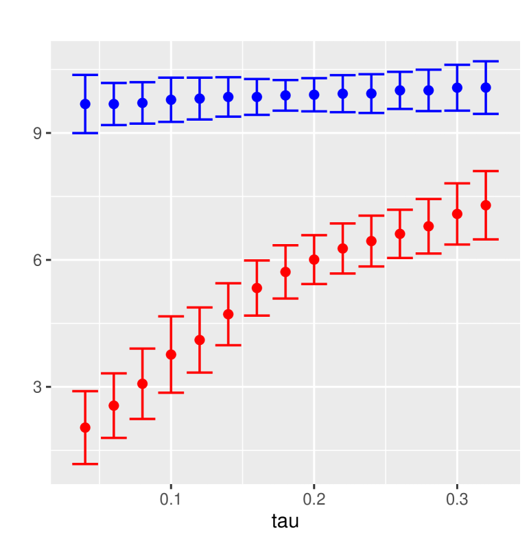
Figure 1: Prediction intervals of the logarithm residual lifetime with $t_{0}=1200$ over different quantile levels of $\tau$ for the selected patient 1 (in blue color) and patient 2 (in red color).

Note that the estimates of $\theta_{\tau,t_{0}}^{(1)}$ in Table 5 do not increase as $\tau$ increases, suggesting a crossing quantile problem in the analysis. Thus we further use a rearrangement procedure proposed by Chernozhukov et al., (2010) to construct a monotone quantile curve, denoted by $\theta_{\tau,t_{0}}^{(k)*}$ in the table. It can be seen from this table that patients with smoke hobby and higher values of BMI, SYSBP and TOTCHOL face higher risks and have shorter remaining time until the occurrence of severe cardiovascular diseases. Moreover, to illustrate the effects of the rearrangement procedure in prediction, we consider $t_{0}=1200$ and calculate the complete estimated $\theta_{\tau,t_{0}}^{(k)*}$ at different quantile levels $\tau$ for both selected patients. Figure 1 visualizes the prediction intervals at different quantile levels for the first and second patients, respectively. Notably, the difference between the two typical patients is quite large at small quantile levels, and lessens as quantile level increases.

6 Discussion

This article introduces a marginal QRL regression approach to address potential correlation among multivariate failure times particularly when there are multiple failure event types or groups of subjects in the study. The estimation process is computationally simple and stable, making it attractive for practical applications. Our proposed variance estimators in Section 3.2 are particularly tailored for the estimator $\widehat{\alpha}_{N}$, which is obtained by solving the estimation equation (6). These asymptotic variance estimators address the within-cluster dependence, making subsequent inference more reliable. This marginal approach is valuable when the relationship between quantile residual lifetimes and covariates is of interest, given that a subject is known to be disease-free at a specific time point. Our proposal leaves the underlying correlation structure completely unspecified, making it robust to potential misspecification and flexible in modeling various multivariate failure times.

The estimating equation (6) is analogous to the well-known generalized estimating equations (GEE) approach with an independent working correlation structure. The GEE method has been extended to quantile regression for longitudinal data in the literature, such as Jung, (1996), Fu and Wang, (2012) and Leng and Zhang, (2014). We adopt the independent working model in light of the considerations as follows. 1) The choice of the working correlation structure should be a trade-off between simplicity and potential efficiency loss from misspecification. 2) Since the association is considered as nuisance in the marginal models, a simpler working correlation will generally suffice, with the independent working structure being recommended by Fahrmeir and Tutz, (2013). Our simulation results demonstrate the promising performance of the proposed method across various dependence structures and copula types.

While we acknowledge that incorporating within-cluster dependence may improve efficiency, integrating the idea of the GEE approach within the framework of the multivariate quantile residual lifetime model poses challenges. As a potential direction for future work, we consider the following weighted estimating equations for residual lifetimes:

$$\frac{1}{n}\sum\limits_{i=1}^{n}\mathbf{X}_{i}^{T}\bm{\mathcal{W}}_{i}^{-1}\bm{\zeta}_{i}=\mathbf{0},$$ (14)

where $\mathbf{X}_{i}=(\mathbf{X}_{i1},\cdots,\mathbf{X}_{im_{i}})^{T}$, $\bm{\zeta_{i}}=(\zeta_{i1},\cdots,\zeta_{im_{i}})^{T}$ with

$$\zeta_{ij}=I(Y_{ij}\geq t_{0})\left[\Delta_{ij}I\left\{Y_{ij}\leq t_{0}+\exp(\mathbf{X}_{ij}^{T}\bm{\alpha})\right\}\widehat{G}(t_{0})/\widehat{G}(Y_{ij})-\tau\right].$$

$\bm{\mathcal{W}}_{i}$ is a working covariance matrix of $\bm{\zeta}_{i}$ and can be expressed as $\bm{\mathcal{W}}_{i}=\bm{\Gamma}_{i}^{\frac{1}{2}}\mathbf{A}_{i}\bm{\Gamma}_{i}^{\frac{1}{2}}$, where $\bm{\Gamma}_{i}=\hbox{diag}\{\sigma^{2}_{i1},\cdots,\sigma^{2}_{im_{i}}\}$ with $\sigma^{2}_{ij}$ being the dispersion of $\zeta_{ij}$. $\mathbf{A}_{i}$ is a correlation matrix that can be specified with some unknown parameters or as a linear combination of some known basis matrices (Qu et al.,, 2000). It is noted that potential issues may arise from (14) demanding more in-depth exploration. First, the dependence may vary with quantile levels or the time points $t_{0}$, making it difficult to specify a proper working correlation structure. Second, as $t_{0}$ increases, the number of individuals with $T_{ij}\geq t_{0}$ will decrease, and the unstable estimation may become more severe for larger $t_{0}$ if an inappropriate correlation structure is imposed. Besides, the potential efficiency gains from incorporating a weight function require further investigation through theoretical justification and numerical studies.

Additionally, we assume the censoring variable $C_{ij}$’s are i.i.d from a distribution independent from $\mathbf{X}_{ij}$. In practice, it may be necessary to verify this assumption about the censoring distribution before applying the proposed method. Our method can be simply improved by incorporating covariates in modeling the censoring times through Cox proportional hazards model for example, and replace $\widehat{G}(\cdot)$ in (6) with $\widehat{G}(\cdot|X)$. Further study of its theoretical justification is also warranted.

Supporting Information

The supplementary material contains an appendix for technical proofs of the lemma and theorems referenced in Section 3 and additional numerical results referenced in Sections 4-5.

Table 1: Estimation results based on 500 replicates for quantile level $\tau=0.5$ under Scenario 1 with Kendall’s tau=0.5.

			$\alpha_{0}(0.5,t_{0})$				$\alpha_{1}(0.5,t_{0})$			runtime
$(n,m)$			$t_{0}=0$	$t_{0}=1$	$t_{0}=2$		$t_{0}=0$	$t_{0}=1$	$t_{0}=2$	(s)
(200,3)	bias		-0.007	-0.009	-0.005		0.008	0.019	0.017
	MCSD		0.146	0.155	0.174		0.235	0.259	0.289
	ASE	IFR	0.130	0.150	0.173		0.235	0.267	0.303
		FR	0.146	0.158	0.178		0.24	0.268	0.303	5.75
		CFS	0.142	0.164	0.196		0.234	0.276	0.332	0.262
		RBS	0.139	0.149	0.167		0.227	0.249	0.281	3.502
	CP	IFR	0.924	0.932	0.942		0.956	0.938	0.958
		FR	0.958	0.95	0.958		0.96	0.958	0.964
		CFS	0.948	0.958	0.964		0.956	0.948	0.98
		RBS	0.95	0.932	0.94		0.946	0.944	0.94
(500,3)	bias		0.002	0.003	0.001		0.004	0.005	0.008
	MCSD		0.087	0.096	0.109		0.138	0.161	0.186
	ASE	IFR	0.082	0.094	0.108		0.147	0.166	0.188
		FR	0.09	0.099	0.11		0.148	0.167	0.188	9.948
		CFS	0.09	0.104	0.122		0.146	0.173	0.206	0.673
		RBS	0.087	0.096	0.106		0.142	0.161	0.178	6.265
	CP	IFR	0.920	0.936	0.952		0.940	0.950	0.963
		FR	0.956	0.956	0.948		0.958	0.96	0.942
		CFS	0.95	0.954	0.978		0.938	0.962	0.98
		RBS	0.946	0.95	0.938		0.954	0.95	0.938
(200,10)	bias		-0.007	-0.003	0		0.004	0.001	-0.002
	MCSD		0.104	0.099	0.105		0.129	0.144	0.163
	ASE	IFR	0.070	0.081	0.092		0.127	0.143	0.159
		FR	0.1	0.102	0.106		0.129	0.147	0.165	10.978
		CFS	0.099	0.105	0.116		0.126	0.151	0.181	0.825
		RBS	0.096	0.098	0.103		0.125	0.141	0.159	6.363
	CP	IFR	0.868	0.906	0.946		0.946	0.952	0.960
		FR	0.954	0.962	0.95		0.954	0.95	0.944
		CFS	0.952	0.972	0.97		0.946	0.966	0.972
		RBS	0.948	0.948	0.944		0.948	0.942	0.932

Table 2: Estimation results based on 500 replicates for quantile level $\tau=0.5$ under Scenario 2.

			$\alpha_{0}(0.5,t_{0})$				$\alpha_{1}(0.5,t_{0})$			runtime
$(n,m)$			$t_{0}=0$	$t_{0}=1$	$t_{0}=2$		$t_{0}=0$	$t_{0}=1$	$t_{0}=2$	(s)
(200,3)	bias		-0.008	-0.002	-0.014		0.003	0.001	0.006
	MCSD		0.174	0.19	0.191		0.313	0.33	0.334
	ASE	IFR	0.131	0.15	0.173		0.238	0.269	0.303
		FR	0.179	0.184	0.164		0.317	0.328	0.291	9.672
		CFS	0.178	0.191	0.179		0.314	0.34	0.315	0.358
		RBS	0.169	0.173	0.154		0.295	0.306	0.268	5.806
	CP	IFR	0.848	0.90	0.929		0.844	0.894	0.927
		FR	0.948	0.94	0.908		0.948	0.944	0.925
		CFS	0.948	0.948	0.939		0.946	0.95	0.946
		RBS	0.936	0.926	0.892		0.936	0.93	0.894
(500,3)	bias		-0.009	-0.009	-0.011		0.011	0.012	0.013
	MCSD		0.109	0.111	0.123		0.197	0.195	0.212
	ASE	IFR	0.082	0.093	0.108		0.148	0.166	0.188
		FR	0.112	0.116	0.118		0.198	0.205	0.208	13.584
		CFS	0.111	0.121	0.129		0.196	0.213	0.227	0.905
		RBS	0.107	0.111	0.114		0.188	0.195	0.199	7.001
	CP	IFR	0.868	0.896	0.909		0.850	0.908	0.909
		FR	0.946	0.966	0.942		0.954	0.96	0.952
		CFS	0.946	0.972	0.963		0.952	0.964	0.969
		RBS	0.932	0.956	0.927		0.942	0.952	0.944
(200,10)	bias		-0.003	-0.002	-0.006		0.002	-0.003	0.002
	MCSD		0.166	0.148	0.142		0.283	0.264	0.256
	ASE	IFR	0.071	0.081	0.094		0.127	0.143	0.163
		FR	0.156	0.147	0.132		0.274	0.262	0.239	14.968
		CFS	0.155	0.153	0.145		0.272	0.273	0.262	0.879
		RBS	0.151	0.142	0.128		0.263	0.254	0.23	7.404
	CP	IFR	0.606	0.692	0.780		0.612	0.708	0.766
		FR	0.926	0.938	0.927		0.938	0.954	0.936
		CFS	0.926	0.946	0.951		0.934	0.964	0.953
		RBS	0.92	0.922	0.91		0.92	0.94	0.925

Table 3: Estimation results based on 500 replicates for quantile level $\tau=0.5$ under Scenario 3.

			$\alpha_{0}(0.5,t_{0})$				$\alpha_{1}(0.5,t_{0})$			runtime
$(n,m)$			$t_{0}=0$	$t_{0}=1$	$t_{0}=2$		$t_{0}=0$	$t_{0}=1$	$t_{0}=2$	(s)
(200,3)	bias		0.003	0.004	-0.003		-0.01	-0.015	-0.009
	MCSD		0.088	0.119	0.165		0.161	0.217	0.296
	ASE	IFR	0.069	0.094	0.133		0.123	0.165	0.235	9.662
		FR	0.092	0.126	0.167		0.163	0.221	0.295	10.724
		CFS	0.092	0.131	0.185		0.161	0.229	0.324	0.445
		RBS	0.09	0.12	0.161		0.158	0.212	0.283	6.031
	CP	IFR	0.884	0.888	0.884		0.856	0.848	0.874
		FR	0.968	0.966	0.956		0.952	0.948	0.936
		CFS	0.968	0.972	0.974		0.948	0.962	0.96
		RBS	0.958	0.962	0.95		0.94	0.928	0.93
(500,3)	bias		-0.001	-0.003	-0.004		0.003	0.005	0.006
	MCSD		0.057	0.077	0.1		0.1	0.136	0.175
	ASE	IFR	0.043	0.057	0.082		0.075	0.101	0.142	21.31
		FR	0.057	0.077	0.104		0.1	0.135	0.18	23.796
		CFS	0.057	0.082	0.115		0.1	0.143	0.2	1.286
		RBS	0.056	0.076	0.101		0.098	0.133	0.175	12.957
	CP	IFR	0.852	0.856	0.88		0.852	0.846	0.892
		FR	0.946	0.946	0.958		0.95	0.952	0.954
		CFS	0.948	0.962	0.97		0.95	0.968	0.97
		RBS	0.94	0.94	0.952		0.944	0.946	0.95
(200,10)	bias		0	-0.001	-0.003		-0.005	-0.008	-0.007
	MCSD		0.075	0.102	0.131		0.131	0.18	0.234
	ASE	IFR	0.037	0.05	0.071		0.065	0.087	0.124	31.27
		FR	0.079	0.108	0.136		0.138	0.189	0.237	35.872
		CFS	0.079	0.114	0.152		0.138	0.198	0.264	1.609
		RBS	0.077	0.105	0.132		0.135	0.183	0.231	13.949
	CP	IFR	0.696	0.688	0.734		0.706	0.684	0.722
		FR	0.966	0.964	0.95		0.948	0.948	0.944
		CFS	0.966	0.972	0.974		0.948	0.96	0.966
		RBS	0.962	0.958	0.942		0.936	0.932	0.944

Table 4: Estimation results based on 500 replicates under Scenario 4 ($n=200,m=10)$).

			$\alpha_{0}(0.25,t_{0})$				$\alpha_{1}(0.25,t_{0})$				$\alpha_{0}(0.5,t_{0})$				$\alpha_{1}(0.5,t_{0})$
$a$			$t_{0}=0$	$t_{0}=1$	$t_{0}=2$		$t_{0}=0$	$t_{0}=1$	$t_{0}=2$		$t_{0}=0$	$t_{0}=1$	$t_{0}=2$		$t_{0}=0$	$t_{0}=1$	$t_{0}=2$
0.1	truth		-0.939	-0.939	-0.939		2.194	2.127	2.09		-0.06	-0.06	-0.06		2.106	2.068	2.044
	bias		-0.009	-0.005	-0.003		-0.003	-0.007	-0.01		-0.005	-0.008	0.002		-0.007	-0.003	-0.013
	MCSD		0.16	0.118	0.15		0.211	0.188	0.218		0.102	0.09	0.108		0.142	0.14	0.157
	ASE	IFR	0.064	0.095	0.144		0.089	0.118	0.163		0.047	0.07	0.106		0.068	0.089	0.122
		FR	0.166	0.116	0.147		0.226	0.186	0.203		0.109	0.091	0.109		0.15	0.138	0.15
		CFS	0.166	0.123	0.162		0.226	0.198	0.225		0.109	0.097	0.12		0.15	0.146	0.166
		RBS	0.155	0.111	0.138		0.213	0.178	0.191		0.106	0.088	0.105		0.145	0.133	0.145
	CP	IFR	0.552	0.89	0.936		0.59	0.768	0.848		0.642	0.878	0.932		0.672	0.782	0.872
		FR	0.954	0.944	0.946		0.964	0.952	0.94		0.97	0.95	0.94		0.962	0.956	0.94
		CFS	0.954	0.952	0.966		0.964	0.96	0.966		0.97	0.96	0.966		0.962	0.96	0.964
		RBS	0.938	0.936	0.928		0.952	0.946	0.92		0.962	0.94	0.93		0.956	0.95	0.928
0.2	truth		-0.939	-0.939	-0.939		2.388	2.276	2.202		-0.06	-0.06	-0.06		2.212	2.148	2.101
	bias		-0.009	-0.005	-0.003		-0.003	-0.007	-0.01		-0.005	-0.008	0.002		-0.005	-0.002	-0.012
	MCSD		0.16	0.118	0.15		0.201	0.183	0.213		0.102	0.09	0.108		0.135	0.134	0.153
	ASE	IFR	0.064	0.095	0.144		0.086	0.115	0.161		0.047	0.07	0.106		0.065	0.086	0.12
		FR	0.165	0.116	0.147		0.215	0.181	0.201		0.109	0.091	0.109		0.143	0.132	0.147
		CFS	0.166	0.123	0.162		0.216	0.192	0.223		0.109	0.097	0.12		0.143	0.14	0.162
		RBS	0.156	0.111	0.138		0.204	0.174	0.191		0.106	0.087	0.105		0.138	0.127	0.141
	CP	IFR	0.554	0.89	0.938		0.596	0.766	0.864		0.642	0.876	0.932		0.672	0.802	0.866
		FR	0.954	0.942	0.946		0.97	0.944	0.94		0.972	0.948	0.94		0.956	0.954	0.948
		CFS	0.954	0.952	0.966		0.97	0.95	0.96		0.972	0.962	0.966		0.956	0.96	0.97
		RBS	0.938	0.936	0.928		0.956	0.936	0.932		0.962	0.938	0.928		0.952	0.944	0.94
0.5	truth		-0.939	-0.939	-0.939		2.97	2.839	2.71		-0.06	-0.06	-0.06		2.53	2.445	2.361
	bias		-0.009	-0.005	-0.003		0.001	-0.004	-0.008		-0.005	-0.008	0.002		-0.002	0.001	-0.01
	MCSD		0.16	0.118	0.15		0.176	0.152	0.185		0.102	0.09	0.107		0.117	0.111	0.131
	ASE	IFR	0.064	0.095	0.144		0.075	0.105	0.153		0.047	0.07	0.106		0.057	0.079	0.113
		FR	0.165	0.116	0.147		0.188	0.152	0.183		0.109	0.091	0.109		0.125	0.112	0.13
		CFS	0.166	0.123	0.162		0.188	0.161	0.203		0.109	0.097	0.12		0.125	0.119	0.143
		RBS	0.156	0.111	0.139		0.177	0.146	0.174		0.105	0.088	0.105		0.12	0.108	0.126
	CP	IFR	0.554	0.89	0.936		0.584	0.838	0.894		0.642	0.876	0.932		0.686	0.858	0.912
		FR	0.954	0.942	0.944		0.968	0.94	0.956		0.972	0.948	0.942		0.966	0.952	0.954
		CFS	0.954	0.952	0.966		0.968	0.954	0.978		0.972	0.962	0.968		0.966	0.958	0.974
		RBS	0.938	0.936	0.928		0.958	0.926	0.94		0.962	0.938	0.93		0.954	0.938	0.942

Table 5: Estimation of regression coefficients and quantile of the residual lifetime $\theta_{\tau,t_{0}}^{(k)}$ ($k=1,2$) for the Framingham heart data with $\tau=0.1,0.2,0.3$ quantiles of ANYCHD/HYPERTEN times after the first examination at $t_{0}=0,1200,2400$ (days), respectively.

		$t_{0}=0$			$t_{0}=1200$				$t_{0}=2400$
		$\tau=0.1$	$\tau=0.2$	$\tau=0.3$		$\tau=0.1$	$\tau=0.2$	$\tau=0.3$		$\tau=0.1$	$\tau=0.2$	$\tau=0.3$
Estimates
Intercept		17.046	14.916	13.862		17.808	14.218	13.071		12.641	12.842	11.446
BMI		-0.045	-0.039	-0.023		-0.076	-0.034	-0.023		-0.021	-0.016	-0.011
SYSBP		-0.045	-0.038	-0.029		-0.046	-0.034	-0.022		-0.033	-0.024	-0.014
CURSMOKE		0.061	0.01	-0.026		0.082	-0.026	-0.051		-0.113	-0.086	-0.053
SEX		0.07	0.077	0.015		-0.014	0.131	0.035		0.253	0.071	0.049
log(TOTCHOL)		-0.512	-0.196	-0.197		-0.536	-0.202	-0.217		-0.093	-0.215	-0.158
$\theta_{\tau,t_{0}}^{(1)}$		10.125	10.171	10.075		10.07	9.932	9.813		9.295	9.543	9.422
$\theta_{\tau,t_{0}}^{(1)*}$		9.973	10.105	10.163		9.785	9.904	10.07		9.295	9.473	9.543
$\theta_{\tau,t_{0}}^{(2)}$		4.699	5.836	6.824		3.763	6.008	7.087		5.846	6.762	7.786
$\theta_{\tau,t_{0}}^{(2)*}$		4.699	5.836	6.824		3.763	6.008	7.087		5.846	6.762	7.786
SE- RBS
(Intercept)		1.161**	0.982**	1.101**		1.686**	1.093**	1.391**		1.382**	1.357**	1.934**
BMI		0.01**	0.009**	0.008**		0.017**	0.011**	0.012*		0.013	0.013	0.016
SYSBP		0.003**	0.003**	0.004**		0.004**	0.004**	0.005**		0.004**	0.004**	0.009
CURSMOKE		0.078	0.066	0.061		0.104	0.068	0.068		0.092	0.069	0.112
SEX		0.069	0.066	0.056		0.106	0.069*	0.075		0.091**	0.071	0.106
log(TOTCHOL)		0.226**	0.185	0.172		0.292*	0.188	0.208		0.266	0.215	0.285
$\theta_{\tau,t_{0}}^{(1)}$		0.158**	0.151**	0.218**		0.267**	0.2**	0.276**		0.216**	0.234**	0.439**
$\theta_{\tau,t_{0}}^{(2)}$		0.231**	0.204**	0.267**		0.461**	0.295**	0.369**		0.317**	0.339**	0.415**
SE- IFR
(Intercept)		1.118**	0.742**	0.562**		1.387**	0.761**	0.617**		1.47**	0.907**	0.539**
BMI		0.01**	0.008**	0.006**		0.016**	0.011**	0.009**		0.014	0.011	0.006*
SYSBP		0.003**	0.002**	0.002**		0.004**	0.002**	0.002**		0.004**	0.002**	0.002**
CURSMOKE		0.077	0.053	0.033		0.109	0.053	0.039		0.114	0.052*	0.028*
SEX		0.079	0.062	0.04		0.115	0.068*	0.053		0.095**	0.072	0.07
log(TOTCHOL)		0.221**	0.143	0.105*		0.282*	0.146	0.117*		0.288	0.166	0.085*
$\theta_{\tau,t_{0}}^{(1)}$		0.134**	0.101**	0.076**		0.182**	0.104**	0.081**		0.207**	0.114**	0.067
$\theta_{\tau,t_{0}}^{(2)}$		0.231**	0.187**	0.138**		0.34**	0.229**	0.175**		0.324**	0.218**	0.185**
* and ** indicate significance at levels 0.1 and 0.05, respectively. The significance is computed based on
RBS/IFR variance estimators.

Supplementary Material for
“Quantile Residual Lifetime Regression for Multivariate Failure Time Data”

Appendix A Technical Proofs

Proof of Theorem 1.

The strong consistency of $\widehat{\bm{\alpha}}_{N}$ can obtained from Lévy’s theorem (Resnick,, 2019), Lemma 2.2 of White, (1980) and Theorem 5.9 of Van der Vaart, (2000). In detail, it remains to verify 1) $||S_{N}(\bm{\alpha})-\overline{S}_{N}(\bm{\alpha})||\rightarrow_{a.s.}0$ uniformly for all $\bm{\alpha}\in\mathcal{D}$; 2) $\inf\limits_{\bm{\alpha}:||\bm{\alpha}-\bm{\alpha}_{0}||=\epsilon}||\overline{S}_{N}(\bm{\alpha})||$ is strictly positive for any $\epsilon>0$. By Conditions 1-2, the proof of the former result is similar to the proof of consistency under an independent case, readers can refer to the appendix in Li et al., (2016). We now show the latter result. From the model (3) and the fact that $\operatorname{Pr}\left\{T_{ij}\geq t_{0}+\exp(\mathbf{X}_{ij}^{T}\bm{\alpha}_{0})|\mathbf{X}_{ij}\right\}-(1-\tau)\operatorname{Pr}\left\{T_{ij}\geq t_{0}|\mathbf{X}_{ij}\right\}=0$, we can see that

$$\begin{split}&\operatorname{Pr}\left\{T_{ij}\geq t_{0}+\exp(\mathbf{X}_{ij}^{T}\bm{\alpha})|\mathbf{X}_{ij}\right\}-(1-\tau)\operatorname{Pr}\left\{T_{ij}\geq t_{0}|\mathbf{X}_{ij}\right\}\\ &=\operatorname{Pr}\left\{T_{ij}\geq t_{0}+\exp(\mathbf{X}_{ij}^{T}\bm{\alpha})|\mathbf{X}_{ij}\right\}-\operatorname{Pr}\left\{T_{ij}\geq t_{0}+\exp(\mathbf{X}_{ij}^{T}\bm{\alpha}_{0})|\mathbf{X}_{ij}\right\}\\ &=\operatorname{Pr}({\color[rgb]{0,0,0}e_{ij}^{\tau}}\geq\mathbf{X}_{ij}^{T}(\bm{\alpha}-\bm{\alpha}_{0})|\mathbf{X}_{ij})-\operatorname{Pr}({\color[rgb]{0,0,0}e_{ij}^{\tau}}\geq 0|\mathbf{X}_{ij})\\ &=F_{e}(0|\mathbf{X}_{ij})-F_{e}(\mathbf{X}_{ij}^{T}(\bm{\alpha}-\bm{\alpha}_{0})|\mathbf{X}_{ij})\\ &=f_{e}(0|\mathbf{X}_{ij})\mathbf{X}_{ij}^{T}(\bm{\alpha}-\bm{\alpha}_{0}).\end{split}$$

Thus, by Conditions 1 and 3, $\inf\limits_{\bm{\alpha}:||\bm{\alpha}-\bm{\alpha}_{0}||=\epsilon}||\overline{S}_{N}(\bm{\alpha})||>0$ for any $\epsilon>0$. We now have completed the proof of the consistency of the proposed estimator under the multivariate setting. ∎

Proof of Lemma 1.

$N^{1/2}S_{N}(\bm{\alpha}_{0})$ can be expressed as

$$\begin{split}&N^{1/2}S_{N}(\bm{\alpha}_{0})=N^{-1/2}\sum\limits_{i}\psi_{i}(\bm{\alpha}_{0})\\ &+N^{-1/2}\sum\limits_{i}\sum\limits_{j}\mathbf{X}_{ij}{\color[rgb]{0,0,0}\Delta_{ij}}I\left\{t_{0}\leq Y_{ij}\leq t_{0}+\exp(\mathbf{X}_{ij}^{T}\bm{\alpha}_{0})\right\}\Bigg{[}\frac{\widehat{G}(t_{0})}{\widehat{G}(Y_{ij})}-\frac{G(t_{0})}{G(Y_{ij})}\Bigg{]},\end{split}$$ (A.1)

where

$$\psi_{i}(\bm{\alpha})=\sum\limits_{j=1}^{m_{i}}\mathbf{X}_{ij}I(Y_{ij}\geq t_{0})\left[\frac{{\color[rgb]{0,0,0}\Delta_{ij}}I\left\{Y_{ij}\leq t_{0}+\exp(\mathbf{X}_{ij}^{T}\bm{\alpha})\right\}}{G(Y_{ij})/G(t_{0})}-\tau\right].$$

The second term in (A.1) involves the estimator of $G$ and can be represented by virtue of martingale processes. We see from (Fleming and Harrington,, 2013) that

$$\widehat{G}_{n}(s)-G(s)=-G(s)\dfrac{1}{N}\sum_{i}\int_{-\infty}^{s}\dfrac{dM_{i}(u)}{y(u)}+o(1)$$ (A.2)

where $M_{i}(u)=\sum_{j}I(Y_{ij}\leq u,{\color[rgb]{0,0,0}\Delta_{ij}}=0)-\int_{0}^{u}I(Y_{ij}\geq t)d\wedge_{G}(t)$ and at-risk indicator $y(u)=\lim_{n\rightarrow\infty}N^{-1}\sum_{i,j}I(Y_{ij}\geq u)$, $\bm{\wedge}_{G}(u)$ is the cumulative hazard function of the censoring variables $C_{ij}$. Through simple algebraic manipulations, (A.1) can be written as

$$N^{1/2}S_{N}(\bm{\alpha}_{0})=N^{-1/2}\sum\limits_{i}\bm{\omega}_{i}(\bm{\alpha}_{0})+o(1),$$ (A.3)

where $\bm{\omega}_{i}(\bm{\alpha})=\psi_{i}(\bm{\alpha})+\eta_{i}(\bm{\alpha})$, and

$$\begin{split}\eta_{i}(\bm{\alpha}_{0})&=\sum\limits_{k,j}\frac{\mathbf{X}_{kj}\delta_{kj}I\left\{t_{0}\leq Y_{kj}\leq t_{0}+\exp(\mathbf{X}_{kj}^{T}\bm{\alpha}_{0})\right\}}{NG(Y_{kj})/G(t_{0})}\int_{t_{0}}^{Y_{kj}}\dfrac{dM_{i}(u)}{y(u)}.\end{split}$$

By Condition 1, the Lyapunov central limit theorem and martingale central limit theorem, the distribution of $N^{1/2}S_{N}(\bm{\alpha}_{0})$ is asymptotically normal with mean zero and covariance matrix $\Sigma=N^{-1}\sum_{i=1}^{n}\bm{\omega}_{i}(\bm{\alpha}_{0})\bm{\omega}_{i}(\bm{\alpha}_{0})^{T}$. ∎

Proof of Theorem 2.

As seen from the proof of Lemma 1, $NS_{N}(\bm{\alpha})$ is asymptotically equivalent to sums of independent random vectors, $\bm{\omega}_{i}(\bm{\alpha})$, we then explore the limiting distribution of $\widehat{\bm{\alpha}}_{N}$ based on the asymptotic properties of $\bm{\omega}_{i}(\bm{\alpha})=\psi_{i}(\bm{\alpha})+\eta_{i}(\bm{\alpha})$. Since $\widehat{\bm{\alpha}}_{N}$ satisfies $S_{N}(\widehat{\bm{\alpha}}_{N})=o(N^{-1/2})$, we see that

$$\begin{split}\sum\limits_{i=1}^{n}\psi_{i}(\widehat{\bm{\alpha}}_{N})&=\sum\limits_{i=1}^{n}\sum\limits_{j=1}^{m_{i}}\mathbf{X}_{ij}I(Y_{ij}\geq t_{0})\left[\frac{{\color[rgb]{0,0,0}\Delta_{ij}}I\left\{Y_{ij}\leq t_{0}+\exp(\mathbf{X}_{ij}^{T}\widehat{\bm{\alpha}}_{N})\right\}}{G(Y_{ij})/G(t_{0})}-\tau\right]\\ &=o(N^{1/2})+\sum\limits_{i}\sum\limits_{j}\mathbf{X}_{ij}{\color[rgb]{0,0,0}\Delta_{ij}}I\left\{t_{0}\leq Y_{ij}\leq t_{0}+\exp(\mathbf{X}_{ij}^{T}\widehat{\bm{\alpha}}_{N})\right\}\Bigg{[}\frac{G(t_{0})}{G(Y_{ij})}-\frac{\widehat{G}(t_{0})}{\widehat{G}(Y_{ij})}\Bigg{]}\\ &=o(N^{1/2})-\sum\limits_{i=1}^{n}\eta_{i}(\widehat{\bm{\alpha}}_{N})+o(1),\end{split}$$

where the second equality is derived from substituting $S_{N}(\widehat{\bm{\alpha}}_{N})$ into, the third is from Equation (A.1). Note that $\bm{\omega}_{i}(\bm{\alpha})$’s are independent and $\sum\limits_{i=1}E\bm{\omega}_{i}(\bm{\alpha})=N\overline{S}_{N}(\bm{\alpha})$. Thus, by Condition 4, we have $\sum\limits_{i=1}^{n}\bm{\omega}_{i}(\widehat{\bm{\alpha}}_{N})=o(n^{1/2})$, which is same as (2.1) in He and Shao, (1996). Using the similar techniques in Wang and Fygenson, (2009), we also denote $u_{i}(\bm{\alpha},d)=\sup\limits_{||\bm{\gamma}-\bm{\alpha}||\leq d}||\bm{\omega}_{i}(\bm{\gamma})-\bm{\omega}_{i}(\bm{\alpha})||$. According to He and Shao, (1996), it remains to show conditions B3-B4, B5’ and B8 in their Theorem 2 are satisfied under our setting.

B3. Denote $\widetilde{e}_{ij}(\bm{\alpha})=\log(Y_{ij}-t_{0})-\mathbf{X}_{ij}^{T}\bm{\alpha}$,$e_{ij}(\bm{\alpha})=\log(T_{ij}-t_{0})-\mathbf{X}_{ij}^{T}\bm{\alpha}$. By the fact that $\sup\limits_{t\leq t_{u}}|\widehat{G}(t)-G(t)|=o(N^{-1/2+\epsilon})$ for any $\epsilon>0$, we see that for $||\bm{\alpha}-\bm{\alpha}_{0}||\leq d_{0}$ and $d\leq d_{0}$,

$$\begin{split}&u_{i}(\bm{\alpha},d)\\ &=\sup\limits_{||\bm{\gamma}-\bm{\alpha}||\leq d}\Bigg{|}\Bigg{|}\sum\limits_{j}\mathbf{X}_{ij}{\color[rgb]{0,0,0}\Delta_{ij}}I(T_{ij}\geq t_{0})\frac{\widehat{G}(t_{0})}{\widehat{G}(Y_{ij})}\Bigg{[}I\left\{e_{ij}(\alpha)\leq\mathbf{X}_{ij}^{T}(\bm{\gamma}-\bm{\alpha})\right\}-I\left\{e_{ij}(\alpha)\leq 0\right\}\Bigg{]}\Bigg{|}\Bigg{|}\\ &\leq c_{1}\sum\limits_{j}||\mathbf{X}_{ij}||{\color[rgb]{0,0,0}\Delta_{ij}}I(T_{ij}\geq t_{0})\frac{G(t_{0})}{G(Y_{ij})}\sup\limits_{||\bm{\gamma}-\bm{\alpha}||\leq d}I\left\{e_{ij}(\bm{\alpha})\leq\max(0,\mathbf{X}_{ij}^{T}(\bm{\gamma}-\bm{\alpha})\right\}\\ &\leq c_{1}\sum\limits_{j}||\mathbf{X}_{ij}||{\color[rgb]{0,0,0}\Delta_{ij}}I(T_{ij}\geq t_{0})\frac{G(t_{0})}{G(Y_{ij})}I\left\{e_{ij}(\bm{\alpha})\leq d||\mathbf{X}_{ij}||\right\}\\ &:=c_{1}B_{i},\end{split}$$

for some constant $c_{1}$. From Condition 1, there exists some constant $c_{2}$ such that

$$\begin{split}E(B_{i}^{2}|\mathbf{X}_{ij},T_{ij}\geq t_{0})&\leq n_{i}\left(G(t_{0})\right)^{2}\sum\limits_{j}||\mathbf{X}_{ij}||^{2}\operatorname{Pr}\left\{e_{ij}(\alpha)\leq d||\mathbf{X}_{ij}||\right\}/G(Y_{ij})\\ &\leq c_{2}n_{i}\sum\limits_{j}||\mathbf{X}_{ij}||^{2}\operatorname{Pr}\left\{e_{ij}(\alpha)\leq d||\mathbf{X}_{ij}||\right\}\\ &\leq c_{2}n_{i}\sum\limits_{j}||\mathbf{X}_{ij}||^{2}\left[1+f_{e}(0|\mathbf{X}_{ij})d||\mathbf{X}_{ij}||\right]+O(d^{2})\end{split}$$

Then, results in Condition B3 of He and Shao, (1996) follows by fixing $a_{i}=c_{3}d^{-1}\sqrt{n_{i}\sum\limits_{j}||\mathbf{X}_{ij}||^{2}\left[1+f_{e}(0|\mathbf{X}_{ij})d||\mathbf{X}_{ij}||\right]}$ for some constant $c_{3}$.

B4. Under Conditions 3-4, $A_{n}=\sum\limits_{i}a_{i}=O(n)$, Condition B4 of He and Shao, (1996) can be obtained. Condition B5 follows by taking $d_{n}=n^{-1/4}\log n$.

B8. Taking the Taylor expansion of $\overline{S}_{N}(\bm{\alpha})$ at $\bm{\alpha}_{0}$ yields

$$N^{1/2}(\overline{S}_{N}(\widehat{\bm{\alpha}}_{N})-\overline{S}_{N}(\bm{\alpha}_{0}))=N^{1/2}(\widehat{\bm{\alpha}}_{N}-\bm{\alpha}_{0})\Lambda G(t_{0})+o(1),$$

where $\Lambda$ is defined in Condition 3. Consequently, Condition B8 of He and Shao, (1996) holds.

Therefore, all conditions in Theorem 2.2 of He and Shao, (1996) hold, and we can apply their theorem, yielding the Bahadur representation in the form of

$$\begin{split}&N^{1/2}(\widehat{\bm{\alpha}}_{N}-\bm{\alpha}_{0})=-N^{-1/2}\Lambda^{-1}(G(t_{0}))^{-1}\sum\limits_{i=1}\bm{\omega}_{i}(\bm{\alpha}_{0})+o_{p}(1)\end{split}$$ (A.4)

Thus, by the Lyapunov central limit theorem, $N^{1/2}(\widehat{\bm{\alpha}}_{N}-\bm{\alpha})$ is asymptotically normal with covariance matrix as $\operatorname{Cov}\left\{N^{1/2}(\widehat{\bm{\alpha}}_{N}-\bm{\alpha})\right\}=\widetilde{\Lambda}^{-1}\Sigma\widetilde{\Lambda}^{-1}$, with $\widetilde{\Lambda}=G(t_{0})\Lambda$.

∎

Proof of Theorem 3.

It can be straightforwardly verified that the difference between the perturbed $G^{*}$ and the truth $G$ can be asymptotically represented by sums of independent random processes in analogy to Eq(A.2). Then, given $E(\gamma_{i})=1$, following the arguments in proofs of Lemma 1 and Theorem 2, we can similarly get

$$N^{1/2}(\widehat{\bm{\alpha}}^{*}-\bm{\alpha}_{0})=-N^{-1/2}\Lambda^{-1}(G(t_{0}))^{-1}\sum\limits_{i=1}\gamma_{i}\bm{\omega}_{i}(\bm{\alpha}_{0})+o_{p}(1).$$ (A.5)

When coupled with Eq (A.4), this implies that

$$N^{1/2}(\widehat{\bm{\alpha}}^{*}-\widehat{\bm{\alpha}}_{N})=-N^{-1/2}\Lambda^{-1}(G(t_{0}))^{-1}\sum\limits_{i=1}(\gamma_{i}-1)\bm{\omega}_{i}(\bm{\alpha}_{0})+o_{p}(1).$$ (A.6)

Since $\operatorname{Var}(\gamma_{i})=1$, we have

$$\begin{split}&\operatorname{Cov}\left[N^{-\frac{1}{2}}\sum\limits_{i=1}(\gamma_{i}-1)\bm{\omega}_{i}(\bm{\alpha}_{0})\Bigg{|}\{Y_{ij},{\color[rgb]{0,0,0}\Delta_{ij}},\mathbf{X}_{ij}\}_{i=1,\cdots,n;j=1,\cdots,m_{i}}\right]\\ &=N^{-1}\sum_{i=1}^{n}\bm{\omega}_{i}(\bm{\alpha}_{0})\bm{\omega}_{i}(\bm{\alpha}_{0})^{T}=\Sigma.\end{split}$$

It follows that given observed data, the conditional distribution of $\sqrt{N}(\widehat{\bm{\alpha}}^{*}-\widehat{\bm{\alpha}}_{N})$ is asymptotically equivalent to the unconditional distribution of $\sqrt{N}(\widehat{\bm{\alpha}}_{N}-\bm{\alpha}_{0})$, thereby justifying the perturbation-based covariance estimation procedure.

∎

Appendix B Additional Numerical Results

Scenario 5. We consider a Frank copula model for the error terms, keeping the scheme for data generation the same as in Scenario 2.

Scenario 6. Unlike the exchangeable dependence considered in Scenarios 1-3 and the new Scenario 5, we adopt an AR(1) dependence structure in this scenario. Particularly, the error terms satisfy $\exp(\epsilon_{ij})\sim Exp(1)$ marginally and are jointly modeled by a Guassian copula with AR(1) correlation of $0.7^{|j-k|}$ between $\epsilon_{ij}$ and $\epsilon_{ik}$ for $j\neq k$. All the other setups remain the same as in Scenario 2.

Scenario 7. A cluster-level covariate $x_{ij}=x_{i}$ is considered, where $x_{i}$ is independently generated from a Bernoulli$(0.5)$. The error terms $(\epsilon_{i1},\cdots,\epsilon_{im})$ follow a multivariate normal distribution with mean zero and covariance matrix $0.64\Sigma_{\epsilon}$, where the $(j,k)$-th entry of $\Sigma_{\epsilon}$ is $0.7^{|j-k|}$. The failure time outcomes $T_{ij}$ are generated from the AFT model $\log T_{ij}=\beta_{0}+\beta_{1}x_{i}+\epsilon_{ij}$ with coefficients $\beta_{0}=0.5$ and $\beta_{1}=1$. In this setting, parameters in the QRL model (3) are obtained by

$$\alpha_{0}(\tau,t_{0})=\left\{\begin{array}[]{cc}\beta_{0}+\Phi_{0.8}^{-1}(\tau),&t_{0}=0,\\ \log\Big{\{}-t_{0}+\exp\left[\beta_{0}+\Phi_{0.8}^{-1}\left\{(1-\tau)\Phi_{0.8}(\log t_{0}-\beta_{0})+\tau\right\}\right]\Big{\}},&t_{0}\neq 0,\end{array}\right.$$

$$\alpha_{1}(\tau,t_{0})=\left\{\begin{array}[]{cc}\beta_{1},&t_{0}=0,\\ \log\left\{\frac{-t_{0}+\exp\left[\beta_{0}+\beta_{1}+\Phi_{0.8}^{-1}\left\{(1-\tau)\Phi_{0.8}(\log t_{0}-\beta_{0}-\beta_{1})+\tau\right\}\right]}{-t_{0}+\exp\left[\beta_{0}+\Phi_{0.8}^{-1}\left\{(1-\tau)\Phi_{0.8}(\log t_{0}-\beta_{0})+\tau\right\}\right]}\right\},&t_{0}\neq 0,\end{array}\right.$$

where $\Phi_{0.8}(\cdot)$ is the cumulative distribution function of a zero-mean normal variable with a standard deviation of 0.8.

Scenario 8. The multivariate failure times is generated from the model: $\log T_{ij}=\beta_{0}+\beta_{1}x_{1i}+\beta_{2}x_{2i}+\beta_{3}x_{3ij}+\epsilon_{ij}$, where $x_{1i}\sim\text{Bernoulli}(0.5)$, $x_{2i}\sim\text{Uniform}[0,1]$, $x_{3ij}\sim N(0,1)$, $\beta_{0}=\beta_{1}=0.6$, $\beta_{2}=0.8$, $\beta_{3}=0.4$. The assumption for the error terms is the same as in Scenario 2. Under this setup, $\alpha_{0}(\tau,t_{0})=\log[-\lambda^{-1}\log(1-\tau)]+\beta_{0}$, $\alpha_{1}(\tau,t_{0})=\beta_{1}$, $\alpha_{2}(\tau,t_{0})=\beta_{2}$ and $\alpha_{3}(\tau,t_{0})=\beta_{3}$.

Estimation results under Scenarios 5-7 are summarized in Table S.3, which consistently highlight the outperformance of the proposed marginal method in addressing diverse dependence structures for multivariate failure times even based on an independent working model. These promising findings further exhibit a degree of robustness of the method across different types of copula. Simulation results for Scenario 8, summarized in Table S.4, also demonstrate that the overall performance of the proposed estimators is promising compared to the IFR estimator. Particularly, its superiority for the coefficients associated with cluster-level covariates $x_{1i}$ and $x_{2i}$ is greater than for the individual-level covariate $x_{3ij}$.

Table S.1: Estimation results based on 500 replicates for quantile level $\tau=0.5$ under Scenario 1 with Kendall’s tau=0.

			$\alpha_{0}(0.5,t_{0})$				$\alpha_{1}(0.5,t_{0})$			runtime
$(n,m)$			$t_{0}=0$	$t_{0}=1$	$t_{0}=2$		$t_{0}=0$	$t_{0}=1$	$t_{0}=2$	(s)
(200,3)	bias		-0.013	-0.011	-0.015		0.026	0.024	0.028
	MCSD		0.13	0.147	0.17		0.238	0.263	0.29
	ASE	IFR	0.129	0.148	0.175		0.231	0.261	0.300
		FR	0.132	0.15	0.176		0.236	0.267	0.305	5.523
		CFS	0.128	0.156	0.191		0.23	0.273	0.327	0.285
		RBS	0.126	0.143	0.165		0.224	0.251	0.284	3.665
	CP	IFR	0.946	0.946	0.971		0.952	0.946	0.958
		FR	0.96	0.95	0.958		0.95	0.962	0.958
		CFS	0.946	0.954	0.978		0.952	0.954	0.972
		RBS	0.944	0.94	0.936		0.936	0.942	0.944
(500,3)	bias		-0.001	-0.003	-0.01		0.006	0.01	0.015
	MCSD		0.081	0.092	0.112		0.148	0.164	0.191
	ASE	IFR	0.082	0.094	0.109		0.148	0.166	0.188
		FR	0.082	0.092	0.107		0.147	0.163	0.186	10.104
		CFS	0.081	0.098	0.119		0.146	0.173	0.206	0.683
		RBS	0.08	0.089	0.103		0.142	0.157	0.178	6.714
	CP	IFR	0.952	0.958	0.959		0.948	0.938	0.943
		FR	0.96	0.954	0.934		0.95	0.956	0.946
		CFS	0.952	0.964	0.968		0.946	0.946	0.97
		RBS	0.95	0.946	0.922		0.944	0.946	0.938
(200,10)	bias		-0.004	-0.006	-0.004		0.009	0.014	0.011
	MCSD		0.071	0.079	0.092		0.127	0.136	0.155
	ASE	IFR	0.071	0.082	0.092		0.128	0.145	0.161
		FR	0.071	0.081	0.091		0.128	0.143	0.159	11.762
		CFS	0.07	0.085	0.101		0.127	0.149	0.176	1.207
		RBS	0.069	0.079	0.089		0.124	0.139	0.153	6.511
	CP	IFR	0.952	0.952	0.962		0.964	0.968	0.964
		FR	0.94	0.958	0.95		0.95	0.96	0.952
		CFS	0.948	0.962	0.972		0.964	0.968	0.976
		RBS	0.938	0.944	0.942		0.946	0.954	0.946

Table S.2: Estimation results based on 500 replicates for quantile level $\tau=0.5$ under Scenario 1 with Kendall’s tau=0.8.

			$\alpha_{0}(0.5,t_{0})$				$\alpha_{1}(0.5,t_{0})$			runtime
$(n,m)$			$t_{0}=0$	$t_{0}=1$	$t_{0}=2$		$t_{0}=0$	$t_{0}=1$	$t_{0}=2$	(s)
(200,3)	bias		-0.011	-0.007	-0.023		0.022	0.014	0.017
	MCSD		0.145	0.154	0.177		0.229	0.253	0.28
	ASE	IFR	0.127	0.147	0.171		0.23	0.259	0.295
		FR	0.151	0.171	0.16		0.237	0.27	0.255	5.905
		CFS	0.15	0.178	0.176		0.232	0.279	0.275	0.288
		RBS	0.143	0.162	0.15		0.223	0.251	0.236	3.603
	CP	IFR	0.914	0.95	0.935		0.94	0.956	0.957
		FR	0.958	0.976	0.921		0.954	0.964	0.931
		CFS	0.956	0.978	0.947		0.942	0.974	0.945
		RBS	0.954	0.96	0.919		0.934	0.946	0.911
(500,3)	bias		0.003	0.006	0.007		0	-0.006	-0.005
	MCSD		0.091	0.113	0.124		0.143	0.174	0.198
	ASE	IFR	0.082	0.094	0.107		0.147	0.166	0.187
		FR	0.096	0.108	0.113		0.149	0.17	0.181	10.822
		CFS	0.095	0.113	0.123		0.147	0.176	0.196	0.636
		RBS	0.093	0.104	0.108		0.143	0.163	0.173	5.685
	CP	IFR	0.926	0.892	0.908		0.954	0.926	0.945
		FR	0.96	0.934	0.923		0.956	0.926	0.936
		CFS	0.958	0.948	0.947		0.952	0.936	0.949
		RBS	0.952	0.928	0.915		0.944	0.924	0.919
(200,10)	bias		0.001	0.001	-0.005		0.003	0.004	-0.005
	MCSD		0.112	0.124	0.131		0.122	0.144	0.178
	ASE	IFR	0.069	0.081	0.092		0.125	0.142	0.16
		FR	0.114	0.126	0.121		0.13	0.155	0.162	13.032
		CFS	0.113	0.131	0.134		0.127	0.159	0.176	0.765
		RBS	0.108	0.12	0.116		0.127	0.15	0.156	6.002
	CP	IFR	0.776	0.8	0.822		0.948	0.938	0.921
		FR	0.954	0.944	0.932		0.956	0.948	0.935
		CFS	0.954	0.958	0.955		0.952	0.956	0.955
		RBS	0.944	0.93	0.926		0.952	0.944	0.917

Table S.3: Estimation results based on 500 replicates for quantile level $\tau=0.5$ under Scenarios 5-7 ($n=200,m=10$).

			$\alpha_{0}(0.5,t_{0})$				$\alpha_{1}(0.5,t_{0})$			runtime
Scenario			$t_{0}=0$	$t_{0}=1$	$t_{0}=2$		$t_{0}=0$	$t_{0}=1$	$t_{0}=2$	(s)
5	bias		-0.002	-0.006	-0.006		0.001	0.011	0.012
	MCSD		0.16	0.159	0.163		0.286	0.281	0.284
	ASE	IFR	0.071	0.081	0.093		0.129	0.144	0.163	32.295
		FR	0.16	0.157	0.162		0.282	0.277	0.284	27.902
		CFS	0.161	0.165	0.18		0.282	0.292	0.314	1.234
		RBS	0.155	0.151	0.156		0.27	0.265	0.273	11.775
	CP	IFR	0.6	0.684	0.748		0.598	0.682	0.75
		FR	0.956	0.954	0.95		0.954	0.952	0.946
		CFS	0.956	0.96	0.964		0.954	0.966	0.97
		RBS	0.954	0.94	0.936		0.952	0.942	0.94
6	bias		0.002	0	-0.007		-0.006	-0.007	0.001
	MCSD		0.113	0.106	0.121		0.203	0.194	0.213
	ASE	IFR	0.069	0.081	0.099		0.122	0.141	0.167	31.735
		FR	0.116	0.113	0.125		0.204	0.199	0.215	36.391
		CFS	0.116	0.12	0.139		0.203	0.21	0.238	1.888
		RBS	0.113	0.111	0.122		0.197	0.194	0.209	19.061
	CP	IFR	0.754	0.872	0.898		0.742	0.86	0.866
		FR	0.97	0.966	0.968		0.96	0.95	0.96
		CFS	0.968	0.97	0.98		0.956	0.966	0.978
		RBS	0.958	0.96	0.964		0.948	0.946	0.942
7	bias		-0.006	-0.012	-0.009		0.008	0.013	0.011
	MCSD		0.059	0.086	0.099		0.082	0.11	0.132
	SE	IFR	0.033	0.057	0.083		0.049	0.073	0.101	29.449
		FR	0.057	0.08	0.1		0.082	0.108	0.129	28.179
		CFS	0.056	0.085	0.112		0.082	0.114	0.143	1.384
		RBS	0.056	0.078	0.097		0.08	0.106	0.125	14.203
	CP	IFR	0.744	0.798	0.896		0.764	0.816	0.874
		FR	0.936	0.942	0.948		0.952	0.958	0.946
		CFS	0.936	0.956	0.966		0.952	0.966	0.976
		RBS	0.932	0.924	0.942		0.95	0.95	0.94

Table S.4: Estimation results based on 500 replicates for quantile level $\tau=0.5$ under Scenario 8.

			$\alpha_{0}(0.5,t_{0})$				$\alpha_{1}(0.5,t_{0})$				$\alpha_{2}(0.5,t_{0})$				$\alpha_{3}(0.5,t_{0})$
$(n,m)$			$t_{0}=0$	$t_{0}=1$	$t_{0}=2$		$t_{0}=0$	$t_{0}=1$	$t_{0}=2$		$t_{0}=0$	$t_{0}=1$	$t_{0}=2$		$t_{0}=0$	$t_{0}=1$	$t_{0}=2$
(200,3)	bias		-0.015	-0.006	-0.012		0.005	-0.003	0.008		0.016	0.014	0.007		0.004	0.005	0.001
	MCSD		0.195	0.206	0.243		0.17	0.179	0.204		0.296	0.307	0.351		0.066	0.084	0.099
	ASE	IFR	0.151	0.18	0.214		0.138	0.159	0.184		0.242	0.277	0.323		0.07	0.081	0.094
		FR	0.203	0.211	0.233		0.184	0.189	0.204		0.322	0.329	0.357		0.07	0.082	0.095
		CFS	0.196	0.212	0.245		0.179	0.192	0.217		0.309	0.333	0.379		0.067	0.082	0.1
		RBS	0.191	0.199	0.219		0.174	0.177	0.191		0.3	0.308	0.336		0.069	0.081	0.095
	CP	IFR	0.882	0.918	0.924		0.882	0.926	0.928		0.884	0.928	0.924		0.956	0.948	0.954
		FR	0.962	0.954	0.95		0.968	0.96	0.954		0.962	0.966	0.956		0.958	0.952	0.958
		CFS	0.952	0.956	0.96		0.964	0.96	0.97		0.954	0.966	0.97		0.944	0.948	0.966
		RBS	0.942	0.942	0.938		0.952	0.95	0.934		0.952	0.942	0.94		0.95	0.946	0.958
(500,3)	bias		-0.007	-0.006	-0.004		0.005	0	-0.006		0.002	0.009	0.016		0.003	0.005	0.002
	MCSD		0.127	0.13	0.144		0.119	0.123	0.126		0.195	0.193	0.21		0.044	0.052	0.062
	ASE	IFR	0.092	0.111	0.133		0.085	0.099	0.115		0.148	0.173	0.2		0.044	0.051	0.059
		FR	0.126	0.132	0.146		0.115	0.119	0.129		0.199	0.207	0.224		0.044	0.052	0.059
		CFS	0.124	0.135	0.157		0.113	0.122	0.139		0.195	0.212	0.241		0.043	0.053	0.065
		RBS	0.12	0.126	0.141		0.11	0.115	0.124		0.189	0.198	0.214		0.043	0.051	0.06
	CP	IFR	0.85	0.92	0.928		0.842	0.894	0.924		0.86	0.934	0.938		0.936	0.94	0.932
		FR	0.944	0.954	0.952		0.94	0.934	0.958		0.962	0.968	0.97		0.936	0.946	0.932
		CFS	0.942	0.958	0.966		0.932	0.95	0.972		0.962	0.972	0.978		0.934	0.954	0.946
		RBS	0.936	0.948	0.94		0.924	0.932	0.938		0.958	0.96	0.958		0.934	0.94	0.932
(200,10)	bias		-0.006	-0.01	-0.011		-0.001	-0.002	-0.003		-0.005	0.004	0.01		0.001	-0.001	0.001
	MCSD		0.175	0.152	0.15		0.161	0.143	0.142		0.28	0.252	0.244		0.037	0.043	0.051
	ASE	IFR	0.08	0.097	0.115		0.074	0.086	0.099		0.128	0.15	0.174		0.037	0.044	0.051
		FR	0.175	0.161	0.16		0.159	0.147	0.144		0.274	0.256	0.253		0.038	0.046	0.053
		CFS	0.172	0.166	0.174		0.157	0.153	0.158		0.269	0.265	0.276		0.037	0.047	0.058
		RBS	0.165	0.155	0.155		0.151	0.142	0.139		0.261	0.244	0.244		0.038	0.046	0.054
	CP	IFR	0.636	0.81	0.862		0.642	0.752	0.836		0.636	0.754	0.834		0.94	0.954	0.952
		FR	0.944	0.958	0.978		0.96	0.962	0.95		0.944	0.962	0.97		0.944	0.958	0.958
		CFS	0.938	0.97	0.984		0.956	0.972	0.974		0.94	0.968	0.986		0.94	0.958	0.976
		RBS	0.932	0.95	0.968		0.946	0.962	0.942		0.932	0.956	0.96		0.944	0.958	0.96

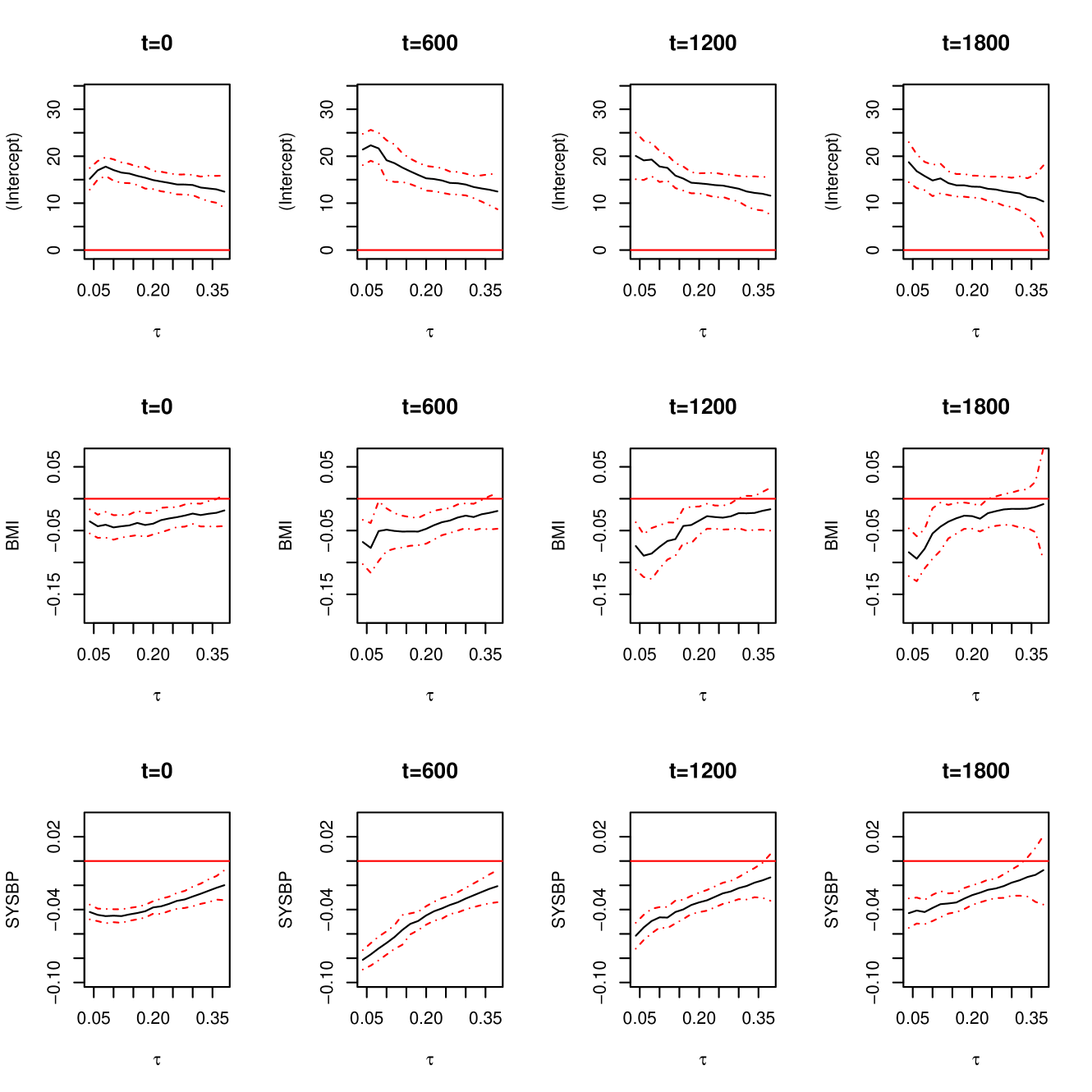
Figure S.1: Estimation results with different quantile levels and residual time points for the Framingham heart data.

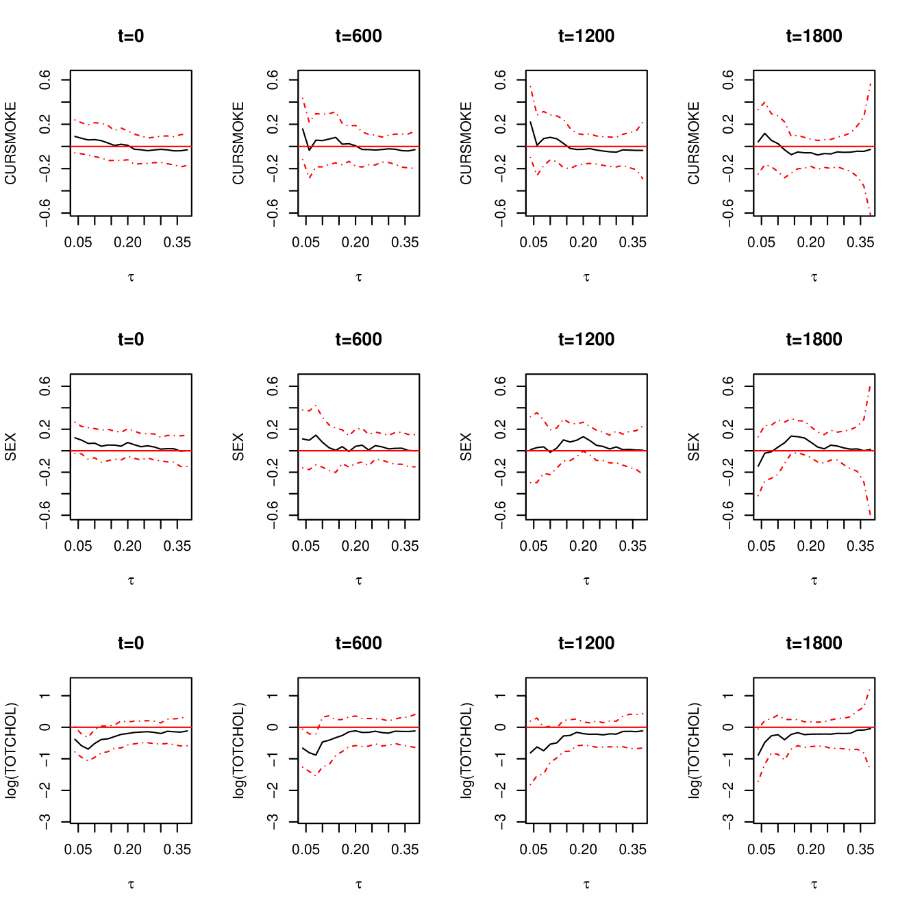
Figure S.2: Estimation results with different quantile levels and residual time points for the Framingham heart data.

References

- Aalen, (1988) Aalen, O. O. (1988). Heterogeneity in survival analysis. Statistics in medicine, 7(11):1121–1137.
- Cai and Prentice, (1995) Cai, J. and Prentice, R. L. (1995). Estimating equations for hazard ratio parameters based on correlated failure time data. Biometrika, 82(1):151–164.
- Caplan et al., (2005) Caplan, D. J., Cai, J., Yin, G., and White, B. A. (2005). Root canal filled versus non-root canal filled teeth: A retrospective comparison of survival times. Journal of Public Health Dentistry, 65(2):90–96.
- Chen et al., (2010) Chen, Y., Chen, K., and Ying, Z. (2010). Analysis of multivariate failure time data using marginal proportional hazards model. Statistica Sinica, 20(33):1025–1041.
- Chernozhukov et al., (2010) Chernozhukov, V., Fernández-Val, I., and Galichon, A. (2010). Quantile and probability curves without crossing. Econometrica, 78(3):1093–1125.
- Chiou et al., (2015) Chiou, S. H., Kang, S., and Yan, J. (2015). Semiparametric accelerated failure time modeling for clustered failure times from stratified sampling. Journal of the American Statistical Association, 110(510):621–629.
- Conner et al., (2022) Conner, S. C., Beiser, A., Benjamin, E. J., LaValley, M. P., Larson, M. G., and Trinquart, L. (2022). A comparison of statistical methods to predict the residual lifetime risk. European Journal of Epidemiology, pages 1–22.
- Csörgő and Horváth, (1983) Csörgő, S. and Horváth, L. (1983). The rate of strong uniform consistency for the product-limit estimator. Zeitschrift für Wahrscheinlichkeitstheorie und verwandte Gebiete, 62(3):411–426.
- Diabetic Retinopathy Study Research Group, (1976) Diabetic Retinopathy Study Research Group (1976). reliminary report on effects of photocoagulation therapy. American Journal of Ophthalmology, 81(4):383–396.
- Duchateau and Janssen, (2008) Duchateau, L. and Janssen, P. (2008). The frailty model. Springer.
- Fahrmeir and Tutz, (2013) Fahrmeir, L. and Tutz, G. (2013). Multivariate Statistical Modelling Based on Generalized Linear Models. Springer Science & Business Media.
- Fleming and Harrington, (2013) Fleming, T. R. and Harrington, D. P. (2013). Counting processes and survival analysis. John Wiley & Sons.
- Fu and Wang, (2012) Fu, L. and Wang, Y.-G. (2012). Quantile regression for longitudinal data with a working correlation model. Computational Statistics & Data Analysis, 56(8):2526–2538.
- Galvao et al., (2023) Galvao, A. F., Parker, T., and Xiao, Z. (2023). Bootstrap inference for panel data quantile regression. Journal of Business & Economic Statistics, 0:1–12.
- Goh and Knight, (2009) Goh, S. C. and Knight, K. (2009). Nonstandard quantile-regression inference. Econometric Theory, 25(5):1415–1432.
- Hagemann, (2017) Hagemann, A. (2017). Cluster-robust bootstrap inference in quantile regression models. Journal of the American Statistical Association, 112(517):446–456.
- Hall and Sheather, (1988) Hall, P. and Sheather, S. J. (1988). On the distribution of a studentized quantile. Journal of the Royal Statistical Society: Series B (Statistical Methodology), 50(3):381–391.
- He et al., (2024) He, W., Yi, G. Y., and Yuan, A. (2024). Analysis of multivariate survival data under semiparametric copula models. Canadian Journal of Statistics, 52(2):380–413.
- He and Shao, (1996) He, X. and Shao, Q.-M. (1996). A general bahadur representation of m-estimators and its application to linear regression with nonstochastic designs. The Annals of Statistics, 24(6):2608–2630.
- Hendricks and Koenker, (1992) Hendricks, W. and Koenker, R. (1992). Hierarchical spline models for conditional quantiles and the demand for electricity. Journal of the American statistical Association, 87(417):58–68.
- Huang et al., (2019) Huang, R., Xiang, L., and Ha, I. D. (2019). Frailty proportional mean residual life regression for clustered survival data: A hierarchical quasi-likelihood method. Statistics in Medicine, 38(24):4854–4870.
- Jeong, (2014) Jeong, J.-H. (2014). Statistical inference on residual life. Springer.
- Jeong et al., (2008) Jeong, J.-H., Jung, S.-H., and Costantino, J. P. (2008). Nonparametric inference on median residual life function. Biometrics, 64(1):157–163.
- Jin et al., (2003) Jin, Z., Lin, D., Wei, L., and Ying, Z. (2003). Rank-based inference for the accelerated failure time model. Biometrika, 90(2):341–353.
- Jin et al., (2006) Jin, Z., Lin, D., and Ying, Z. (2006). Rank regression analysis of multivariate failure time data based on marginal linear models. Scandinavian Journal of Statistics, 33(1):1–23.
- Jung, (1996) Jung, S.-H. (1996). Quasi-likelihood for median regression models. Journal Of the American Statistical Association, 91(433):251–257.
- Jung et al., (2009) Jung, S.-H., Jeong, J. H., and Bandos, H. (2009). Regression on quantile residual life. Biometrics, 65(4):1203–1212.
- Kim et al., (2012) Kim, M.-O., Zhou, M., and Jeong, J.-H. (2012). Censored quantile regression for residual lifetimes. Lifetime data analysis, 18:177–194.
- Koenker, (2005) Koenker, R. (2005). Quantile regression. Cambridge university press.
- Kwon et al., (2022) Kwon, S., Ha, I. D., Shih, J.-H., and Emura, T. (2022). Flexible parametric copula modeling approaches for clustered survival data. Pharmaceutical Statistics, 21(1):69–88.
- Leng and Zhang, (2014) Leng, C. and Zhang, W. (2014). Smoothing combined estimating equations in quantile regression for longitudinal data. Statistics and Computing, 24(1):123–136.
- Li et al., (2016) Li, R., Huang, X., and Cortes, J. (2016). Quantile residual life regression with longitudinal biomarker measurements for dynamic prediction. Journal of the Royal Statistical Society Series C: Applied Statistics, 65(5):755–773.
- Li and Peng, (2015) Li, R. and Peng, L. (2015). Quantile regression adjusting for dependent censoring from semicompeting risks. The Journal of the Royal Statistical Society, Series B (Statistical Methodology), 77(1):107–130.
- Liang and Zeger, (1986) Liang, K.-Y. and Zeger, S. L. (1986). Longitudinal data analysis using generalized linear models. Biometrika, 73(1):13–22.
- Lin, (2014) Lin, D. (2014). Marginal models for multivariate survival data. Wiley StatsRef: Statistics Reference Online.
- Lin et al., (2019) Lin, X., Li, R., Yan, F., Lu, T., and Huang, X. (2019). Quantile residual lifetime regression with functional principal component analysis of longitudinal data for dynamic prediction. Statistical Methods Medical Research, 28(4):1216–1229.
- Ma and Wei, (2012) Ma, Y. and Wei, Y. (2012). Analysis on censored quantile residual life model via spline smoothing. Statistic Sinina, 22(1):47–68.
- Othus and Li, (2010) Othus, M. and Li, Y. (2010). A gaussian copula model for multivariate survival data. Statistics in biosciences, 2:154–179.
- Peng and Huang, (2008) Peng, L. and Huang, Y. (2008). Survival analysis with quantile regression models. Journal of the American Statistical Association, 103(482):637–649.
- Portnoy and Koenker, (1997) Portnoy, S. and Koenker, R. (1997). The gaussian hare and the laplacian tortoise: computability of squared-error versus absolute-error estimators. Statistical Science, 12(4):279–300.
- Powell, (1991) Powell, J. L. (1991). Estimation of monotonic regression models under quantile restrictions. In Nonparametric and Semiparametric Models in Econometrics. Cambridge University Press.
- Qu et al., (2000) Qu, A., Lindsay, B. G., and Li, B. (2000). Improving generalised estimating equations using quadratic inference functions. Biometrika, 87(4):823–836.
- Resnick, (2019) Resnick, S. I. (2019). A probability path. Springer Science & Business Media.
- Tsao and Vasan, (2015) Tsao, C. W. and Vasan, R. S. (2015). The Framingham Heart Study: past, present and future. International Journal of Epidemiology, 44(6):1763–1766.
- Van der Vaart, (2000) Van der Vaart, A. W. (2000). Asymptotic statistics. Cambridge university press.
- Wang et al., (2019) Wang, H. J., Feng, X., and Dong, C. (2019). Copula-based quantile regression for longitudinal data. Statistica Sinica, 29:245–264.
- Wang and Fygenson, (2009) Wang, H. J. and Fygenson, M. (2009). Inference for censored quantile regression models in longitudinal studies. The Annals of Statistics, 37(2):756–781.
- Wang and Li, (2013) Wang, H. J. and Li, D. (2013). Estimation of extreme conditional quantiles through power transformation. Journal of the American Statistical Association, 108(503):1062–1074.
- Wang et al., (2012) Wang, H. J., Li, D., and He, X. (2012). Estimation of high conditional quantiles for heavy-tailed distributions. Journal of the American Statistical Association, 107(500):1453–1464.
- Wang and Wang, (2009) Wang, H. J. and Wang, L. (2009). Locally weighted censored quantile regression. Journal of the American Statistical Association, 104(487):1117–1128.
- White, (1980) White, H. (1980). Nonlinear regression on cross-section data. Econometrica, 48(3):721–746.
- Xu et al., (2023) Xu, Y., Zeng, D., and Lin, D. (2023). Marginal proportional hazards models for multivariate interval-censored data. Biometrika, 110(3):815–830.
- Yin and Cai, (2005) Yin, G. and Cai, J. (2005). Quantile regression models with multivariate failure time data. Biometrics, 61(1):151–161.
- Ying et al., (1995) Ying, Z., Jung, S. H., and Wei, L. J. (1995). Survival analysis with median regression models. Journal of the American Statistical Association, 90(429):178–184.
- Yu et al., (2021) Yu, T., Xiang, L., and Wang, H. J. (2021). Quantile regression for survival data with covariates subject to detection limits. Biometrics, 77(2):610–621.
- Zeng and Lin, (2008) Zeng, D. and Lin, D. Y. (2008). Efficient resampling methods for nonsmooth estimating functions. Biostatistics, 9(2):355–363.
- Zhou and Jeong, (2011) Zhou, M. and Jeong, J.-H. (2011). Empirical likelihood ratio test for median and mean residual lifetime. Statistics in Medicine, 30(2):152–159.