Speculative Ad-hoc Querying

Abstract.

Analyzing large datasets requires responsive query execution, but executing SQL queries on massive datasets can be slow. This paper explores whether query execution can begin even before the user has finished typing, allowing results to appear almost instantly. We propose SpeQL, a system that leverages Large Language Models (LLMs) to predict likely queries based on the database schema, the user’s past queries, and their incomplete query. Since exact query prediction is infeasible, SpeQL speculates on partial queries in two ways: 1) it predicts the query structure to compile and plan queries in advance, and 2) it precomputes smaller temporary tables that are much smaller than the original database, but are still predicted to contain all information necessary to answer the user’s final query. Additionally, SpeQL continuously displays results for speculated queries and subqueries in real time, aiding exploratory analysis. A utility/user study showed that SpeQL improved task completion time, and participants reported that its speculative display of results helped them discover patterns in the data more quickly. In the study, SpeQL improves user’s query latency by up to $289\times$ and kept the overhead reasonable, at $\$4$ per hour.

1. Introduction

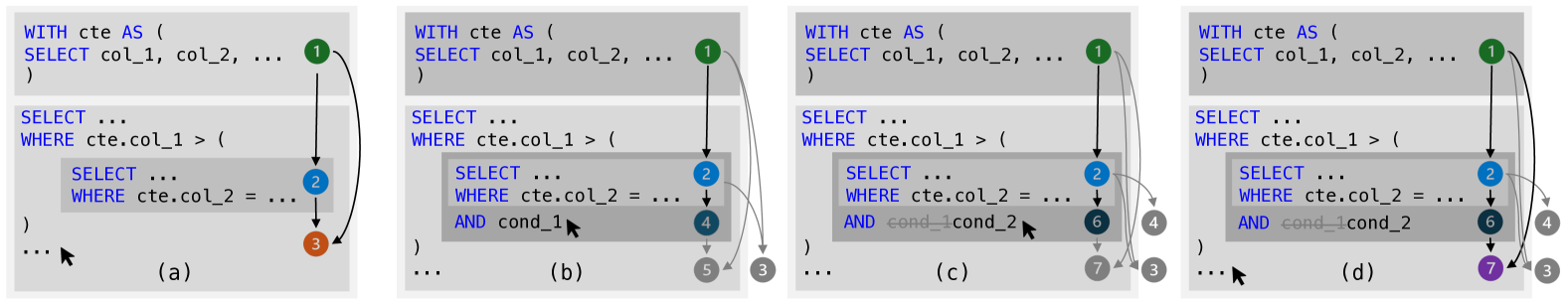
Figure 1. SpeQL’s workflow as the user edits the query. Each node represents a SELECT statement. SpeQL structures these nodes as a directed acyclic graph (DAG) and schedules their execution. The colored nodes indicate precomputed subqueries, while the result of the user’s highlighted (cursor-placed) query is previewed to the user.

Millions of business intelligence (BI (BIsurvey, )) users and tens of thousands of data warehouse (DW (DWSurvey, )) customers rely on interactive data exploration to discover insights that drive decision making. It is important to minimize the latency between when a user submits a query and when the results are displayed to them. Often, an unplanned, ad-hoc analytical query takes 10s of seconds or minutes. A database systems that reduces the latency to milliseconds can not only reduce friction, but even cause a user to discover useful insights in the data that they may have missed otherwise simply due to the latency in running every query (liu2014effects, ). The challenge is that datasets can span hundreds of gigabytes and queries can be complex and reference multiple tables. Faster computation may not be possible, even with the best techniques and optimizations.

This paper proposes speculative ad-hoc querying, a new avenue of speedup opened by Large Language Models (LLMs), and presents a system SpeQL, that precomputes the result while the user is typing, even before the user submits their SQL query. The challenge is that it is almost impossible, for LLMs and humans alike, to exactly predict everything a user will write, especially constants; thus simply autocompleting their query and executing it does not work. Consider a user incrementally constructing the following SQL query:

a: SELECT item FROM sales WHERE price > 5 AND  quantity > 50

b: SELECT item FROM sales WHERE price > 5 AND quantity > 10 

c: SELECT item FROM sales WHERE price > 5 AND quantity > 1 

While the LLM generates structurally and contextually relevant completion (grey in a), it rarely exactly matches the final query c. Instead of striving for perfect predictions, SpeQL prompts LLMs to generate standard code fixes and completions and uses logical rules to rewrite the SQL query and precompute portions of the data structures (see the next paragraph). This enables near-instantaneous results once the user finishes writing the query.

SpeQL exploits precomputation in both query planning/compilation and in execution. For planning/compilation, it suffices to predict the common query structures which will remain effective even if some conditions are different. To ensure the execution is also useful, SpeQL tries to predict a superset of the user’s intended query. As long as the final query belongs to the subset, the precomputation will be useful. For example, as the user types step a above, SpeQL postprocesses the LLM completion and issues:

d: CREATE TEMPORARY TABLE tb AS

SELECT item, quantity FROM sales WHERE price > 5;

This command runs asynchronously while the user continues editing. Assume the conditions are selective, when step b is completed, SpeQL issues

e: SELECT item FROM tb WHERE quantity > 10;

The query structure of e is simpler than b, allowing SpeQL to simplify planning and compilation. In addition, the execution uses the temporary table tb in d, much smaller than the original table sales. Finally, the user changes the constant and submits c, SpeQL rewrites the final query as

f: SELECT item FROM tb WHERE quantity > 1;

This shares the same structure as e, enabling the database to reuse the execution plan, further reducing planning/compilation time. For more complex queries, such as those involving subqueries or common table expressions (CTEs), SpeQL decomposes the query into multiple reusable temporary tables, structuring them as a directed acyclic graph (DAG), and schedules their creation accordingly.

The use of LLMs accounts for three patterns in how humans write ad-hoc queries. First, incomplete queries are rarely syntactically correct or parsable, even with an error-correcting parser. Second, users may not follow a predefined structure to write their query. Third, users may progressively add column or table names to the query. Precomputation on such a query will not be useful component for the future query, which is substantial in reality (shute2024sql, ).

The ability to perform speculative ad-hoc querying quickly allows SpeQL to offer another useful feature with minimal overhead: if the user’s cursor is placed over a subquery in the main query that they are constructing, SpeQL displays the result of the query in its UI. This ability to interactively peek at the intermediate results helps users debug their code and get desired data earlier. Naturally, the intermediate results are the result of speculation. To ensure that the user is always aware of exactly what the displayed results mean, the UI displays the speculated part of the code as an intuitive diff, seamlessly integrating with AI completion tools.

To assess SpeQL’s impact on user workflow, we conducted an IRB exempt utility/user study where 24 participants were given two questions to be answered using SQL queries. It showed that SpeQL presents significant ($p<0.05$) and effective speedup on a designed data exploration task, and 87.5% of the recruited participants agree SpeQL improves their productivity. Readers can access our SpeQL service (with demo) through a publicly accessible VS Code plugin.

SpeQL bears a strong resemblance to speculative execution in other domains, such as incremental search in search engines, and branch prediction and cache-line prefetching in CPUs. Instead of speculating on program execution, SpeQL uses LLMs to speculate on user’s coding behavior. As with any speculation, SpeQL is more expensive to run than a system that does not speculate. However, we incorporate mechanisms to reduce cost. When tuned to maximize performance and cost, it costs $1 per hour for LLMs and up to $3 per hour for query execution.

This paper makes two key contributions:

• We propose the concept of speculative ad-hoc querying, leveraging LLMs to guide speculative query execution and reduce latency when constructing analytical queries.

• We implement SpeQL, the first system for speculative ad-hoc querying on $O(100GB)$ analytical query workloads. Integrated with LLM speculation, SQL rewriting and scheduling, and UI/UX, SpeQL ensures efficient and end-to-end coordination among LLM inference, database processing, and user input. Leveraging open source parsing and transpiling functionalities, SpeQL can support multiple industrial-strength SQL engines, such as Amazon Redshift, Snowflake, Microsoft Synapse, Google BigQuery, among others. Through experiments on 103 industry-standard TPC-DS (tpcds, ) queries at a 100GB scale using Amazon Redshift, SpeQL reduces P90 planning latency by 94.42% (1.22 seconds), compilation latency by 99.99% (6.43 seconds), and execution latency by 87.23% (3.34 seconds), with a reasonable (7.72 seconds) P90 execution overhead. The improvements hold consistently for smaller (10GB) and larger (1000GB) datasets. We open source SpeQL as well as a plug-and-play VS Code extension on GitHub https://github.com/lihy0529/SpeQL.

2. Example of SpeQL Execution

Before describing the workings of SpeQL, we illustrate its functionality by running the TPC-DS Q1 benchmark (tpcds, ), demonstrating the sequence of events as a user types their analytical query.

As shown in Fig. 1 (a), the query contains a common table expression (CTE) and a subquery, with the subquery referencing the CTE. SpeQL decomposes the query into three components: the CTE ①, the subquery ②, and the main query ③. Assume the main query is now incomplete and not parsable. SpeQL tries to first debug the incomplete query by rectifying typos and syntactic errors using LLMs. Then a logic-driven postprocessing is performed to sequentially create temporary tables for these components and previews the result of the main query ③ to the user.

Next, suppose the user finds the subquery misses some conditions from the preview (Fig. 1 (b)). Instead of continuing the main query, they turns to the subquery and adds a filtering condition, cond_1, in it. Upon detecting this change, SpeQL uses the original subquery ② to predict and create a new subquery ④ and quickly previews its result. This is feasible because ④ is a subset of ②. Later, assume the user modifies cond_1 to cond_2, resulting in another new subquery ⑥ (Fig. 1 (c)). Although ⑥ is not a subset of ④, it remains a subset of ②. Consequently, SpeQL uses ② to create ⑥ and is still able to preview the result quickly.

Finally, suppose the user goes back to the main query (Fig. 1 (d)). Due to the subquery modifications of Fig. 1 (b), (c), the main query changes to ⑦. SpeQL re-executes the main query ⑦ based on ① and ⑥. This process also operates on precomputed temporary tables, which are typically smaller and more efficient to process than base tables.

The example highlights several features of SpeQL: (1) By reusing intermediate results, SpeQL minimizes redundant computation, reducing latency and cost. (2) The intermediate results allow users to iteratively refine their queries with immediate insights.

3. SpeQL design

Depending on the prediction accuracy, SpeQL employs three levels of speculative execution, as illustrated in Level 0$\sim$2 of Fig. 2. In the best case (Level 0), the prediction is perfect — for instance, when the user has nearly completed writing the query. In this scenario, SpeQL can precompute the exact query and display it instantly from the result cache on request. In the second-best case (Level 1), the user has entered enough of the query for SpeQL to guess which subset of the data the user is interested in and precompute temporary tables that filter the base data to a more relevant subset. At the earliest stages of query input (Level 2), SpeQL can guess the relevant tables and columns to prefetch data from disk into memory. In another orthogonal dimension of speculation (not shown in the figure), SpeQL can preplan and precompile queries since this only requires it to guess the query structure and not any of the constants. For this, SpeQL uses query planning and compilation caches already present in many relational database systems, such as Amazon Redshift (armenatzoglou2022amazon, ) and IBM DB2 (ibmplancache, ). SpeQL implements the logic that tells the database which temporary tables to compute and how to use them. Our evaluation shows that each type of speculation contributes to SpeQL’s overall performance.

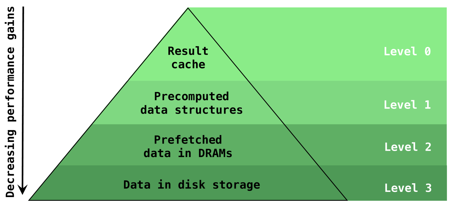
Figure 2. SpeQL proposes a multi-level optimization hierarchy to mitigate varying degrees of misprediction.

To implement these three levels of speculation, SpeQL consists of a pipeline of two components, an LLM-guided speculator (speculator, §3.1) and a logic-driven scheduler (scheduler, §3.2), between the user’s editor and the information retrieval endpoint, i.e., the database (Fig. 3). The speculator retrieves inputs from the editor, predicts a superset SQL query, and forwards it to the scheduler. The scheduler instructs the database to precompute portions of data structures and execute the queries to display intermediate results in the editor. The editor displays a clear, diff-like patch between the input and the speculative query in its UI, ensuring that users always have full visibility into what the displayed results mean.

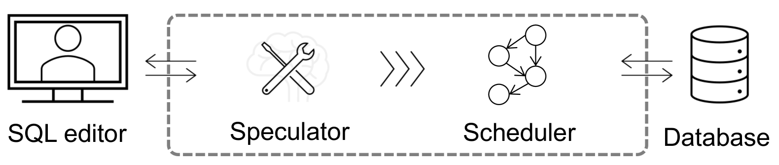
Figure 3. SpeQL’s modular architecture.

3.1. Speculator: predicting a superset

The first component, the speculator, aims to produce a superset SQL query whose results can be reused by the user’s future, possibly more precise, SQL query. It proceeds in three steps: (1) LLM-based debugging of the user input to produce a syntactically and semantically valid SQL query; (2) LLM-based autocompletion to hypothesize the user’s potential future additions; (3) Logic-driven merging of the debugged SQL query and the autocompleted text to form a superset SQL query. To provide necessary context to LLMs, in the first two steps, the speculator enriches the LLM prompts with the database schema (table and column names) and historical SQL queries from a preconfigured Meta FAISS vector database (douze2024faiss, ) using max cosine similarity.

3.1.1. Debugging

The debugging step fixes syntactic or semantic errors in the user’s incomplete query. This uses self-debugging (chen2023teaching, ) with up to $2N$ iterations. An iteration has two steps: (1) A syntax/semantic check (via SQLGlot’s SQL optimizer (mao2024sqlglot, )) that checks whether the query is correct. If it is, debugging is finished. (2) If not, SpeQL shows the current query and the error message to the LLM and instructs it to generate a revised version of the query by making minimal changes to the original. The loop fails if an error-free query is not generated even after $2N$ iterations. In this case, SpeQL decreases $N$ by one (if $N>1$) to save inference cost; otherwise, it restores $N$ to default. The loop often fails in early SQL query writing stages, e.g., when the user has not yet specified the referenced tables in the FROM clause.

3.1.2. Autocompletion

Upon receiving the debugged SQL query, the speculator asks the LLM again to predict what the user may next type in the cursor’s position. If the autocompletion is perfect, prexecuting the speculated SQL query enables the system to return the final result quickly once the SQL query finishes.

3.1.3. Over-projection

However, SpeQL does not really preexecute the autocompleted SQL query because it is inherently imperfect. Directly precomputing the speculated SQL query and storing its result as a temporary table does not work if the final query refers to columns not present in the speculation. This often happens since users can perform conditions on columns (e.g., in WHERE, JOIN clauses) but do not need to SELECT it. A simple fix is to SELECT all columns that might be referenced, but this risks adding too many columns. To address this, SpeQL introduces the concept of over-projection. In general, over-projection means speculating extra columns for SELECT and GROUP BY, but not extra conditions in WHERE, JOIN, or HAVING. We get the extra columns from the autocompleted text, and perform over-projection by adding every feasible column referenced in the autocompleted text to the SELECT and GROUP BY clauses of the debugged SQL query to construct the final superset SQL query.

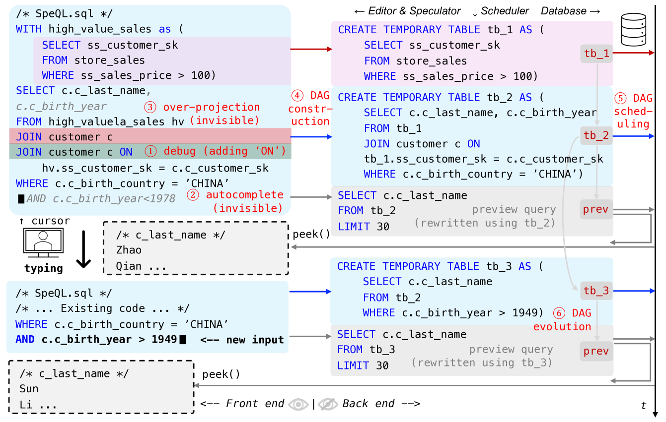
Figure 4. Running example referenced throughout §3. SpeQL fetches user input, using a speculator to debug (①), autocomplete (②), and over-project (③). The scheduler receives the superset query and constructs a DAG of query commands (④), dispatches the commands to precompute data structures or intermediate results (⑤), and evolves the DAG structure as the new input comes (⑥).

3.1.4. Example

When the user composes a SQL query, as depicted in the upper left corner of Fig. 4 (the first blue box), the speculator retrieves the user’s input and performs three steps to produce a superset SQL query: ① Debugging. The speculator debugs the SQL query by modifying ”JOIN customer c” to ”JOIN customer c ON” so that the SQL query is executable. The user can visualize this modification as a diff-like patch in the editor. ② Autocompletion. The speculator autocompletes a new condition ”AND c.c_birth_year > 1978”. This step assumes LLMs can predict the query structure (by prompting LLMs with the database schema and query history, see the initial paragraph of §3.1) but not the exact constants. ③ Over-projection. By string-matching each token in the autocompletion ([AND, c, c_birth_year, 1978]), the speculator identifies one column ”c_birth_year” and adds it to the SELECT clause, making a superset SQL query. This query remains reusable even if the constant (1978) is mispredicted. We explain the remaining parts of this figure in §3.2.

3.1.5. Optimizations.

LLM invocations for debugging can dominate runtime. To reduce the overhead, SpeQL uses two optimizations: (1) As discussed in §3.1.1, SpeQL makes $2N$ attempts to debug. In the first $N-1$ iterations, a small model (here, GPT-4o-mini) is instructed to output a local fix. A local fix is a JSON-formatted “diff file”, e.g., [{"old": "SELECT _col, FROM", "new": "SELECT _col FROM"}]. Producing this requires fewer output tokens than rewriting the query from scratch. In the $N^{th}$ iteration, a large model (here, GPT-4o) attempts a local fix. In the next $N-1$ iterations, the small model attempts complete rewrites. Finally, the large model attempts a complete rewrite. (2) It is inefficient to re-run the debugging every time the user types something. Instead, we cache the diff file from LLM debugging from a previous version of the query and directly apply it to the new version. If the patched query passes SQLGlot’s SQL optimizer (mao2024sqlglot, ) grammar check, we can skip LLM-based debugging entirely.

3.2. Scheduler: dispatching query commands

After receiving the superset query from the speculator, the scheduler decomposes it into multiple SELECT statements and dispatches their execution, creating partial data structures for future use and previewing intermediate results to the user.

3.2.1. DAG construction

For each superset query generated by the speculator (§3.1), the scheduler decomposes it into multiple SELECT statements and maps them to a directed acyclic graph (DAG). Each vertex in the DAG represents a SQL query, in one of two types: The first is a temporary table creation query, representing any SELECT statement augmented with over-projected columns (§3.1.3), converted to CREATE TEMPORARY TABLE statements by removing LIMIT and ORDER BY clauses and adding the CREATE TEMPORARY TABLE header. This way, they can be used as starting points for downstream queries. The second is the preview query, i.e., the most specific SELECT statement where the user’s cursor is placed. This does not have over-projected columns and has a LIMIT NUM_LINES clause to display only a few lines of the result. For example (Fig. 4 ④), the scheduler decomposes the superset query in the upper left corner into two SELECT statements: one for a common table expression (CTE) and one for the main query. Each of them is then mapped to a temporary table creation vertex (tb_1, tb_2) in the upper right of the figure. Because the user’s cursor is positioned within the main query, a third vertex (the gray box) is generated to represent the preview query. Notably, the grey box is an rewritten but equivalent version of the main query. We detail the rewriting algorithm in §3.2.2.

The edges in the DAG encode the input-output dependencies and subsumption dependencies among the vertices. Specifically, an edge exists from vertex $A$ to $B$ if either $A$ is a temporary table that is referred to by B (input-output dependency), or the result of $A$ is a more general or encompassing version of $B$ (subsumption). For example (Fig. 4 ④), in the figure’s upper right corner, an edge is drawn from the pink vertex (CTE) to the blue vertex (main query), because the blue query depends on the result of the CTE; Similarly, an edge connects the blue vertex to the gray vertex since the preview query is a subset of tb_2.

3.2.2. DAG scheduling

The scheduler dispatches the execution of the DAG vertices based on whether the user presses double ENTERs. (1) If SpeQL detects double ENTER key presses, it interprets this as a signal that the user wants immediate execution, prioritizing quick query result display. It first cancels all running jobs. Then it executes and displays the user highlighted (cursor-placed) SELECT statement. If ancestor temporary tables are available, SpeQL uses them. If not, it executes the query directly without creating any additional temporary tables. (2) If the user is typing but has not pressed double ENTERs, we prioritize precomputing the temporary tables. Here, we first execute the ancestors of the preview query, then the preview query, then the non-ancestors. In each category, the scheduler’s execution follows SQLGlot’s (mao2024sqlglot, ) inherent traversing order. A better scheduling order may exist but is future work. For now, we observe that any arbitrary topologically sorted order works well. (we will explain the reason in §3.2.3). Additionally, for each query execution, the scheduler applies a fine grained matching (a.k.a. view matching (halevy2001answering, )) mechanism to maximize the reuse of existing temporary tables. Specifically, it greedily searches the most recent created temporary tables. If the new query $A$ has a subset of projections and a superset of predicates of an existing temporary table $B$, the scheduler rewrites $A$ using $B$. Note that the greedy matching approach does not guarantee that the rewritten SQL is more efficient. For example, X JOIN R (where X = P JOIN Q is precomputed) may not always outperform P JOIN Q JOIN R. A cost-based approach using the database’s cardinality estimator is future work. For now, we observe that the greedy matching algorithm works well (we will explain the reason in §3.2.3).

For example (Fig. 4 ⑤), consider the three vertices shown in the upper right of the figure: (1) The creation of tb_1 (pink); (2) The creation of tb_2 (blue); (3) The preview query (gray). Since the user does not press double ENTERs, the scheduler first executes the ancestors of the preview query — that is, it processes tb_1 and then tb_2 (with tb_1 executed before tb_2 because it is the direct parent). If tb_2 is successfully created, the preview query is rewritten using tb_2 and postprocesses on it; Otherwise (e.g., due to a timeout), the preview query is computed directly from the base tables (not shown in the figure). The resulting preview is then delivered to the user’s editor as a side window (indicated by the first gray dashed box). Since no further non-ancestor vertices, the scheduler idles after the execution of the preview query.

3.2.3. DAG evolution

New input occurs as the user modifies the code, and the scheduler keeps evolving the DAG to match the new input. (1) If the cursor of the new input moves from one SELECT statement to another, or the user adds/deletes new texts, the DAG adds new vertices accordingly (see the example in the next paragraph). This ensures that only one additional temporary table creation vertex is new. This means the DAG scheduling order is often unique, and thus any arbitrary topologically sorted order in §3.2.2 often works. Additionally, since the user’s modifications are usually local, e.g., adding a new filtering condition, so the most recent temporary table is probably the smallest, optimal superset, so the greedy matching algorithm in §3.2.2 works. (2) Statements removed from the query become “grayed out” in the DAG and will not be scheduled for execution. However, any temporary tables already created remain available unless they are explicitly evicted (e.g., due to exceeding memory constraints, see §3.2.4).

Fig. 4 ⑥ is an example. Initially, the scheduler has decomposed the superset query (depicted in the blue upper left box) into three vertices: tb_1 (pink), tb_2 (blue), and the preview query (gray). Suppose the user now appends a new condition ”AND c.c_birth_year > 1949” to the main query. The speculator then generates an updated superset query (illustrated as the blue lower left box). Notice that the common table expression (CTE) remains unchanged; hence, the vertex corresponding to tb_1 persists. (1) Because the main query has been modified, the scheduler creates one new temporary table creation vertex for tb_3 (pink), and updates the preview query (displayed in the lower right gray box). (2) If tb_2 has not yet been created, e.g., due to a timeout, its vertex is removed (”grayed out”), and the dependency edge is reconfigured so that tb_3 depends directly on tb_1 (not shown in the figure). Conversely, if tb_2 is available, it remains active and subsumes tb_3, with an edge drawn from tb_2 to tb_3. Note that tb_2 is the smallest superset of tb_3. After the DAG has evolved, the scheduler returns to the DAG scheduling (⑤) step, waiting for the creation of tb_2, greedily using it to create tb_3, and finally using tb_3 to execute the updated preview query. The resulting output is then delivered to the user (as indicated by the gray dashed box on the lower left).

3.2.4. Optimizations

The scheduler includes several optimizations to make it more efficient and universal. (1) It incorporates abstract syntax tree (AST) level query optimizations for each SQL query. It uses SQLGlot’s SQL optimizer (mao2024sqlglot, ) to eliminate redundant operators and common sub-expressions, and thus simplifies the query structure. (2) Long-running queries are canceled once a predefined timeout is reached. If the query is a temporary table creation command, the scheduler skips it; If it is the preview query, SpeQL reverts to approximate query processing (garofalakis2001approximate, ) via random sampling of rows (a rate of 5% by default) to generate approximate results. This ensures that SpeQL remains responsive even when handling large datasets and computationally expensive queries. (3) It monitors memory usage and evicts the least recently used (LRU) temporary tables when resource limits are reached. We leave the development of eviction policies that consider additional resource metrics for future work.

3.3. Compatibility, privacy, and robustness

SpeQL ensures compatibility across cloud providers and SQL dialects. User preconfigures the input dialect, and SpeQL’s speculator encodes this information into LLM prompts to generate dialect-consistent output. The scheduler transforms the dialect to make it align with the endpoint (using SQLGlot (mao2024sqlglot, )). Further, compared with CREATE MATERIALIZED VIEW (gupta1995maintenance, ) command, SpeQL uses CREATE TEMPORARY TABLE (ben2000temporary, ) command which is widely supported and does not require elevated privileges.

SpeQL respects user privacy by creating only temporary tables, exist solely in the current session, invisible to data administrators and other users (ben2000temporary, ). Currently, SpeQL does not tune data distributions or create indices/tables that persist beyond the current session. SpeQL does not send any actual data to LLMs, enhancing security.

SpeQL guards that only safe commands — SELECT, CREATE/DROP TEMPORARY TABLE commands — can be issued to the database. Temporary tables are evicted when the user closes the current session (the editor), ensuring robustness.

4. Implementation

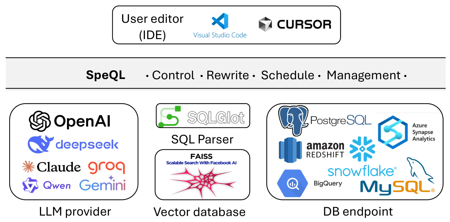
Figure 5. SpeQL serves as an intermediary between the user’s editor and the analytical SQL database.

We implemented SpeQL’s core logic using 8,000 lines of python (3.10.12), and its user interface is implemented as a VS Code ($\geqslant$ v1.90) plugin comprising 1,000 lines of TypeScript. SpeQL is thus an end-to-end agent system that orchestrates large language model (LLM) inference with database execution and human interaction (Fig. 5). In the future, it can be integrated into database management systems (DBMS (ramakrishnan2002database, )), IDE and business intelligence (BIs (negash2008business, )) tools to support engine-specific features like user-defined predicates and projections and incorporate common front-end features such as ordering buttons, column click-and-drag capabilities, data visualization tools, and query recommendations (chatzopoulou2009query, ).

SpeQL supports multiple LLM API providers, including OpenAI, Deepseek, Claude, Groq, Qwen and Gemini, among others, which allows users to choose their preferred models. SpeQL leverages the IndexFlatL2 index in the Meta FAISS vector database (douze2024faiss, ) to store and retrieve the most cosine-similar historical query to enrich LLM prompts, thereby guiding LLMs to generate more contextually relevant outputs.

To support multiple database endpoints such as Redshift, Synapse, BigQuery, and Snowflake, SpeQL uses their Python connectors and SQLGlot (mao2024sqlglot, ) to parse and transpile SQL between them.

5. Evaluation

5.1. Setup

5.1.1. Goal

We evaluate SpeQL’s performance and behavior (§5.2) and its impact on user productivity (§5.3). We do not evaluate SpeQL’s generalization over multiple LLMs and SQL engines, since it is a moving target and is not our primary contribution.

5.1.2. Dataset

We use two sources of SQL queries. First, we use 103 SQL queries from TPC-DS (tpcds, ), a widely used benchmark for online analytical processing (OLAP) workloads (chaudhuri1997overview, ), and accompanying data with scale factors of 10GB, 100GB, and 1000GB. TPC-DS has 103 complex queries that are diverse and stress many aspects of SpeQL’s performance. However, it does not have information on how a human originally typed the query. Thus, we emulate typing by revealing the query’s lines sequentially (line by line), allowing ample time for SpeQL to execute each line before progressing to the next. Our second source of SQL queries is from our user study, which has real typing data from a human using SpeQL to interactively explore the database answer a given analytical question. Here, the typing is realistic, but the queries are not as diverse.

5.1.3. Database endpoint

To accommodate the bursty nature of data exploration, we leverage Amazon Redshift’s serverless architecture with a maximum of 8 RPUs. This ensures that the database cost remains capped at $\$0.375\times 8=\$3$ per hour (redshift_pricing, ). Additionally, we use Redshift Spectrum to enable direct, on-demand querying of the TPC-DS dataset stored in Amazon S3 (TPC-DS_Data, ). This setup is extremely challenging as SpeQL has minimal control over the underlying architecture. However, it also highlights SpeQL’s generalizability across commercial systems with limited extensibility.

5.1.4. LLM API

We uses GPT-4o-2024-08-06 and GPT-4o-mini (OpenAI APIs) for LLM prediction to balance inference quality and cost, and uses text-embedding-3-large to create vector database to record query history. We select OpenAI APIs because they are the most well known, though others like Deepseek V3 (liu2024deepseek, ) and R1 (guo2025deepseek, ) may be more cost-efficient. Note that this paper aims to illustrate opportunities opened by LLMs. Training/fine-tuning/prompting/comparing LLMs are beyond its scope.

5.1.5. Baseline

Since SpeQL is the only one system supporting speculative execution during query construction, we use Amazon Redshift without speculative execution as the baseline.

5.1.6. Metrics

We measure performance using planning time, compilation time, and execution time as our primary metrics, which are three basic components of elapsed query time. To mitigate the impact of cold cache misses, we run all test cases twice, with execution time measured during the second run. However, as Redshift does not provide an option to disable the query compilation cache, planning and compilation time is measured during the first run. We are unable to accurately measure the elapsed time on benchmarking because the three components may overlap.

5.2. Benchmarking

For each query, we incrementally reveal the last 20 lines to SpeQL, one line at a time, to simulate user input behavior, ultimately generating 21 inputs. Upon receiving a new input, we allow SpeQL ample time to run temporary table creation or previewing commands, but each command has an ad-hoc timeout limit based on dataset size: 15 seconds for 10GB, 30 seconds for 100GB, and 60 seconds for 1000GB. We disable result cache because we run each query twice (§5.1.6) and enabling it would have produced spuriously good results for SpeQL. We do not evict created temporary tables so that temporary tables in previous steps remain available for future inputs.

5.2.1. Complex DAG

Our experiments reveal that these intermediate queries construct complex directed acyclic graphs (DAGs), comprising tens of vertices and edges on average, as summarized in Table. 1. Despite this complexity, the total size of temporary tables for each query averages only a few gigabytes, representing a significantly smaller scanning space compared to the base tables, which typically range from tens to thousands of gigabytes. This reduction in scanning space underscores the benefit of precomputation.

10G/100G/1000G	Median	Mean	Max
LOC in queries	39	48.4	227
# of temp tables	8/7/7	10.5/10.1/8.4	52/52/44
# of previews	13/13/11	13.5/13.0/11.0	21/21/21
# of edges	37/36/30	49.6/48.9/39.6	285/285/273
Total size (GB)	2.0/2.8/3.6	5.1/7.5/9.6	33.0/39.0/75.9

Table 1. Benchmarking measurement statistics. “LOC” is short for “lines of code”.

Shape (cnt)	Queries in TPC-DS 100GB
Tree (45)	1, 2, 4, 6, 11, 17, 18, 19, 22, 24, 24 (b), 25, 27, 29, 30, 31, 34, 35, 36, 38, 39, 39 (b), 42, 45, 46, 50, 53, 54, 59, 62, 64, 66, 67, 68, 70, 71, 73, 74, 75, 81, 85, 86, 89, 96, 99
Mesh (21)	10, 14, 14 (b), 28, 33, 44, 51, 56, 58, 60, 61, 65, 69, 76, 78, 80, 83, 87, 88, 90, 97
Linear (37)	3, 5, 7, 8, 9, 12, 13, 15, 16, 20, 21, 23, 23 (b), 26, 32, 37, 40, 41, 43, 47, 48, 49, 52, 55, 57, 63, 72, 77, 79, 82, 84, 91, 92, 93, 94, 95, 98

Table 2. Taxonomy of SpeQL dependency graphs.

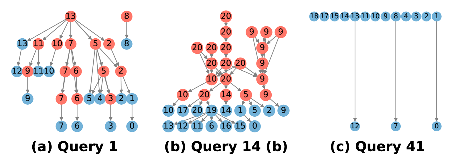
Figure 6. Tree-, mesh-, and linear-like DAGs. Orange vertices represents temporary table creation queries, and blue vertices represents preview queries. The number i represents the vertex created when the last i lines of code are revealed. ”0” indicates that the user has completed typing. DAGs of the remaining 100 TPC-DS (tpcds, ) queries are in Appendix (Fig. 13, 14, 15).

We manually categorize the DAGs into three distinct shapes: tree-like, mesh-like, and linear-like, as summarized in Table. 2. In this taxonomy, tree-like DAGs account for 43.7% of the dataset. They are characterized by numerous filtering (WHERE) conditions and are exemplified by TPC-DS Q1 (Fig. 6 (a)). For these queries, SpeQL can extract data from an initial superset that gradually refines into the final query as the user iterates.

/* TPC-DS Q1 includes many filtering conditions */
SELECT ... WHERE ctr1.ctr_total_return > (...)
AND s_store_sk = ctr1.ctr_store_sk
AND s_state = ‘TN’
AND ctr1.ctr_customer_sk = c_customer_sk ...

As queries grow more modular, exemplified by TPC-DS Q14 (b) (Fig. 6 (b)), the presence of multiple CTEs and subqueries transforms the structure into a mesh-like DAG, representing 20.4% of the dataset. In such cases, SpeQL tries to generate fine-grained temporary tables for each SELECT statement, so that significant changes to a single SELECT statement do not disrupt other statements, preserving their utility as components for future queries.

/* TPC-DS Q14 (b) has multiple CTEs and subqueries */
WITH cte_1 AS (SELECT ... INTERSECT SELECT ... INTERSECT SELECT ...), cte_2 AS (SELECT ... UNION ALL SELECT ... UNION ALL SELECT ...) SELECT ... from (SELECT ... WHERE ss_item_sk IN (SELECT ...) ... HAVING SUM (ss_quantity * ss_list_price) > (SELECT ...) UNION ALL SELECT ... WHERE cs_item_sk IN (SELECT ...) ... HAVING SUM (cs_quantity * cs_list_price) > (SELECT ...) UNION ALL SELECT ... WHERE ws_item_sk IN (SELECT ...) ... HAVING SUM (ws_quantity * ws_list_price) > (SELECT ...)) GROUP BY ROLLUP (...) ORDER BY ... LIMIT 100

Nevertheless, 35.9% of queries result in linear-like DAGs, where SpeQL struggles to precompute partial results, and the reasons are various: (1) In queries like TPC-DS Q13, the presence of non-associative aggregation functions (e.g., AVG ()) render temporary tables ineffective unless predictions are fully accurate. (2) In queries like TPC-DS Q23, SpeQL cannot precompute the long-running subqueries within timeout. (3) In queries like TPC-DS Q41 (Fig. 6 (c)), SpeQL fails to extract meaningful supersets or subqueries/CTEs from an incomplete query (see the code below). Despite these limitations, linear-like queries can still benefit from precompilation and prefetching.

/* TPC-DS Q41 is hard to precompute */
SELECT ... FROM item WHERE
(cond_01 AND (cond_02 AND (cond_03 OR cond_04) AND (cond_05 OR cond_06) AND (cond_07 OR cond_08)) OR
(cond_09 AND (cond_10 AND (cond_11 OR cond_12) AND (cond_13 OR cond_14) AND (cond_15 OR cond_16)) OR ...
(cond_56 AND (cond_57 AND (cond_58 OR cond_59) AND (cond_60 OR cond_61) AND (cond_62 OR cond_63)))
ORDER BY i_product_name LIMIT 100

Clearly, there are strong implications between the query patterns, the resulting DAG and how amenable the query would be to precompute. A progressive refinement pattern (hellerstein2000informix, ) often yields a tree-like DAG, which inherently captures a subsumption relationship between the original query and its subsequent refinements. The success of speculative execution largely hinges on whether new queries align with the precomputed superset; otherwise, the effort is wasted, and the DAG degenerates into a more linear structure. In contrast, in drill-down/roll-up/template-based query patterns (hellerstein2000informix, ), computations are distributed across modular vertices, including CTEs and subqueries. These nodes establish input-output dependencies with the vertex being edited, remain effective even if the superset does not match. A vivid analogy is to compare a mesh-like DAG to a body of modular vertices of CTEs/subqueries, extending into a tree- or linear-like tail. These structures are observed due to the complexity of the query structure. Simple benchmarks like TPC-H (poess2000new, ) cannot uncover this knowledge.

5.2.2. Low latency

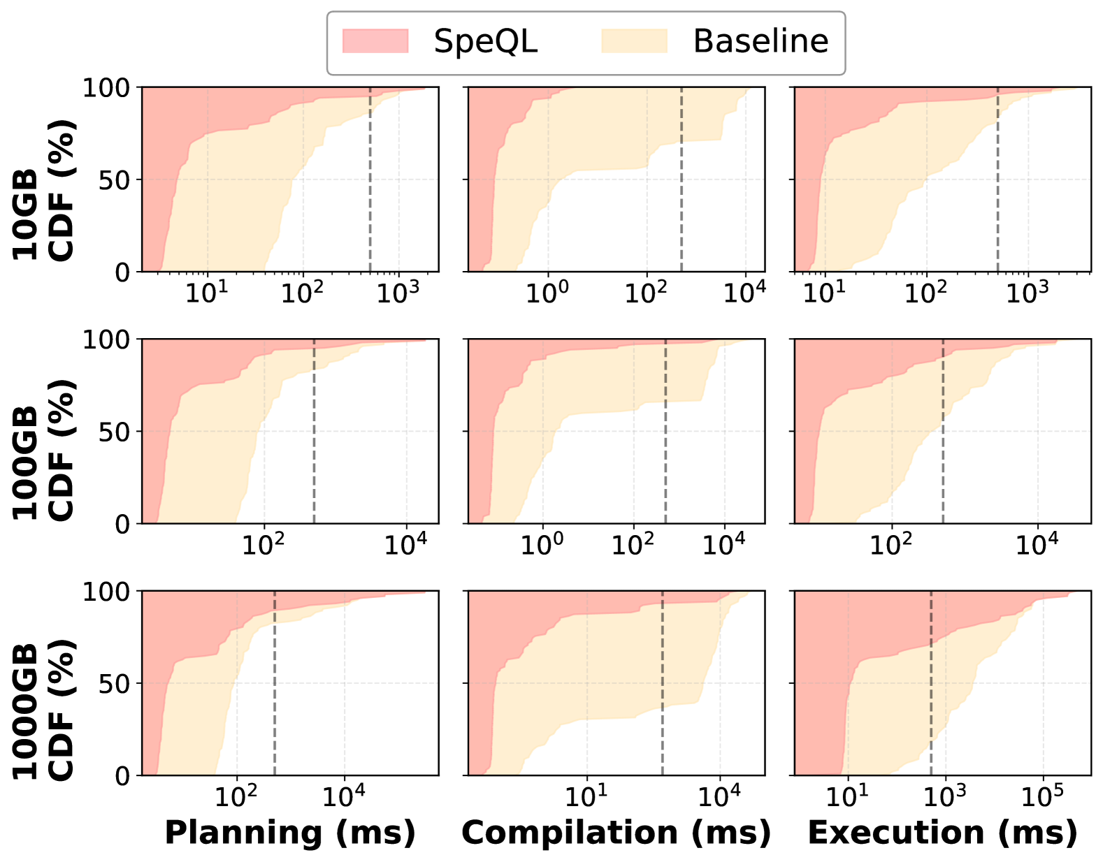
Figure 7. SpeQL significantly reduces query latency. Literature (liu2014effects, ) shows that latency greater than 500ms (vertical dashed lines) significantly degrades user’s performance.

SpeQL reduces latency across metrics and dataset sizes. We independently measured the planning, compilation, and execution latencies for 103 queries in both SpeQL and the baseline. For SpeQL, latency is defined as the time spent from the submission of the final input to the completion of it; For baseline, the latency is exactly the processing time of individual queries. Notably, 12 queries on the 1000GB dataset failed to complete within the predefined 60-second timeout. For these cases, their latencies were recorded as equivalent to the baseline. The results are shown in Fig. 7, where we draw a 500ms threshold, as latencies exceeding this value have been proven to significantly degrade user performance (liu2014effects, ).

We first analyze results on the TPC-DS 10GB benchmark. This size of data simulates exploration for small to medium-sized businesses, which highlights a unique property: query compilation requires significantly more time than planning or execution. Via precompilation, SpeQL reduces the compilation latency from up to 10 seconds to a couple of milliseconds (upper center), and thus reduces the elapsed latency from seconds to milliseconds.

Next, we analyze the 100GB and 1000GB workloads, which simulate medium to medium-large OLAP tasks, where planning, compilation and execution may all be the main factors. At this scale, precomputing temporary tables can not only generate partial results, but the use of temporary table also simplifies the query plan, so that SpeQL is able to cuts not only execution, but also planning and compilation latencies. In our experiments, SpeQL reduces P90 planning latency by 1.22 seconds (-94.42%), compilation latency by 6.43 seconds (-99.99%), and execution latency by 3.34 seconds (-87.23%) on 100GB workload, and reduce P80 planning latency by 0.25 seconds (-53.17%), compilation latency by 10.60 seconds (-99.99%), and execution latency by 23.71 seconds (-89.81%) on 1000GB workload.

While the latency improvements are impressive, they are somewhat exaggerated, as the assumption that user types arbitrarily slowly is, of course, unrealistic. We report more realistic values from our user study with real humans typing queries (§5.3). Our empirical intuition is that SpeQL performs well on $O(100GB)$ datasets but struggles to scale beyond that since query execution time may be much longer than user typing time. That said, sizes ranging from 10GB to 1000GB encompass the majority of practical use cases and query workloads, as highlighted in a well-known yet disputed article “Big Data is Dead” (bigdataisdead, ).

5.2.3. Reasonable overhead

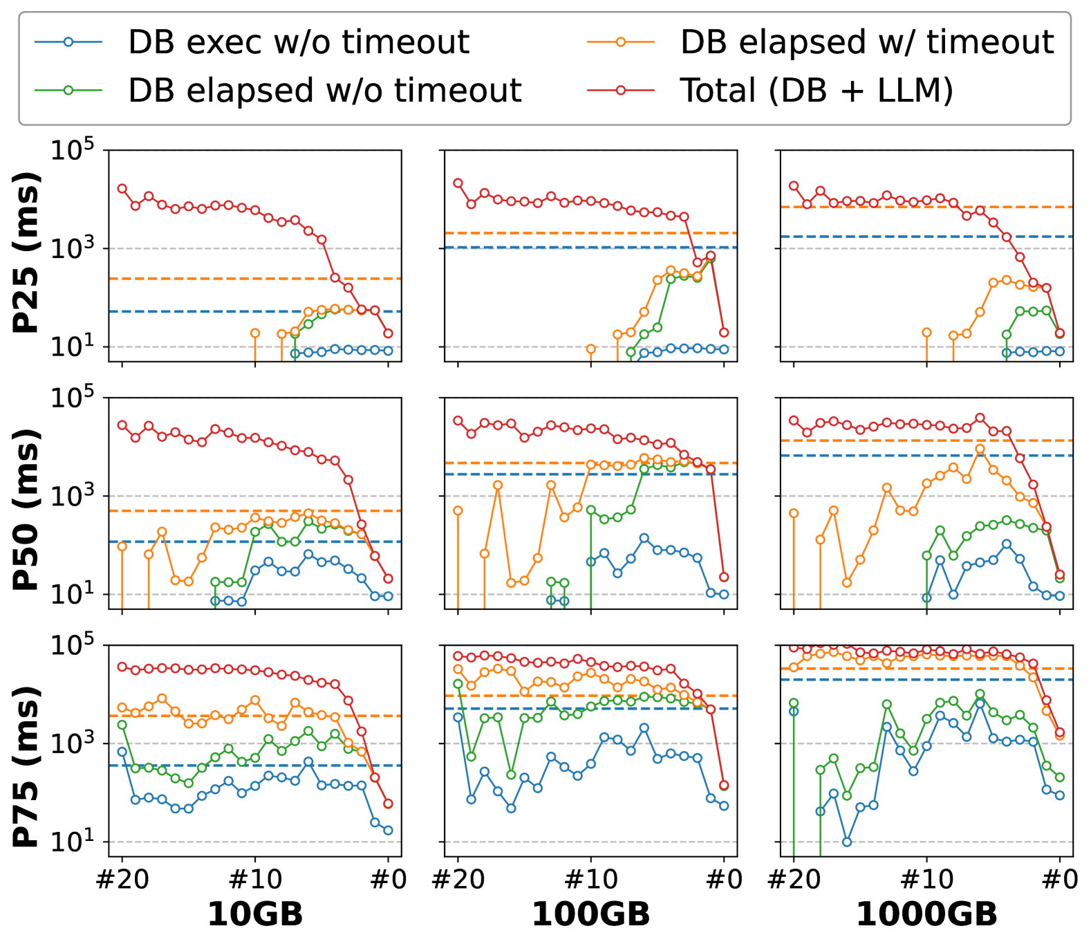
Figure 8. Overhead breakdown for each input. "#i" represents the time spent when the last i lines of code are revealed. The database time encompasses both temporary table creation and preview query running time (we measure them during the first run, see §5.1.6). The blue and green curves exclude timeouts, while the blue curve further omits planning/compilation time. The blue and orange horizontal axis lines are the baseline’s.

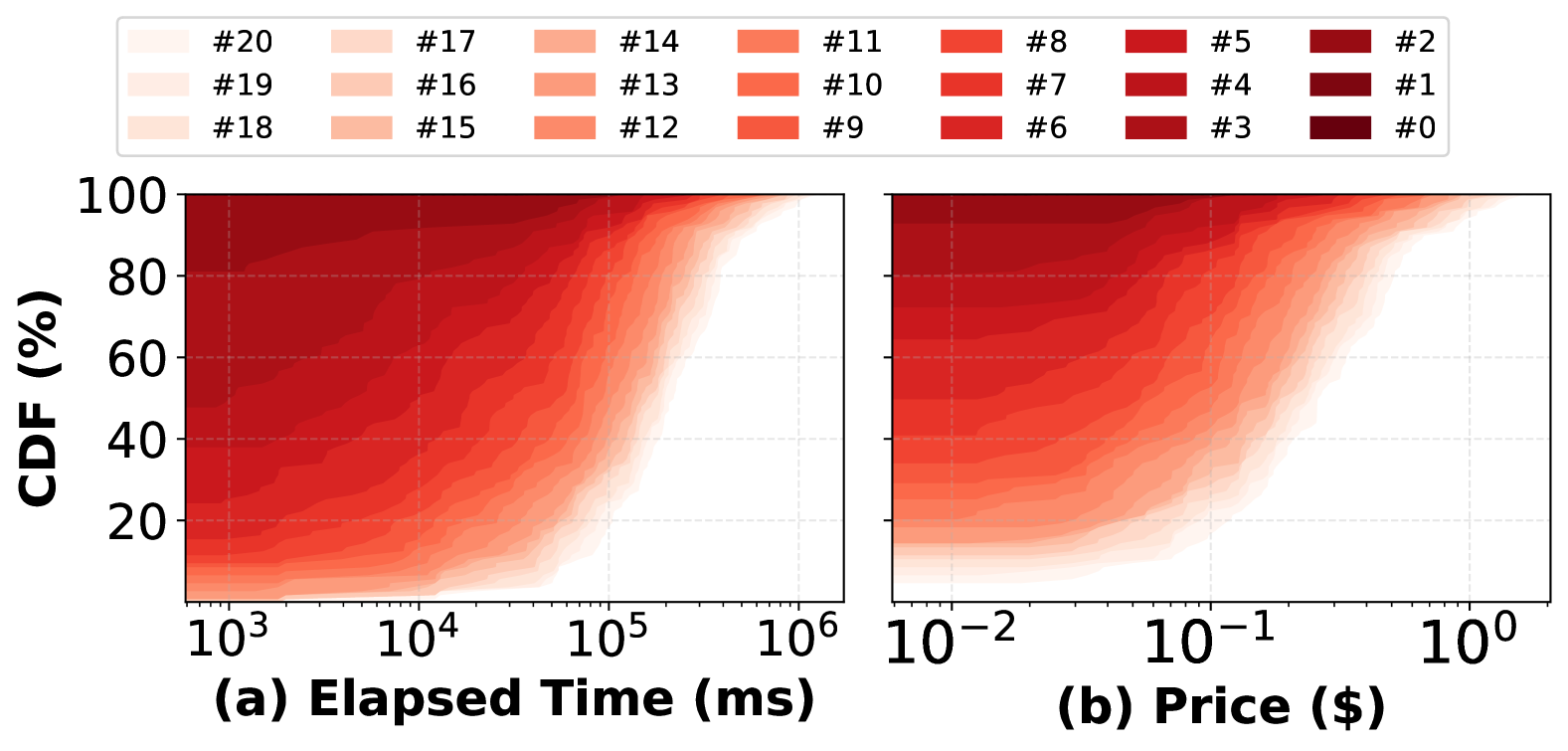
Figure 9. LLM inference overhead. "#i" represents the cumulative time since the last i lines of code are revealed.

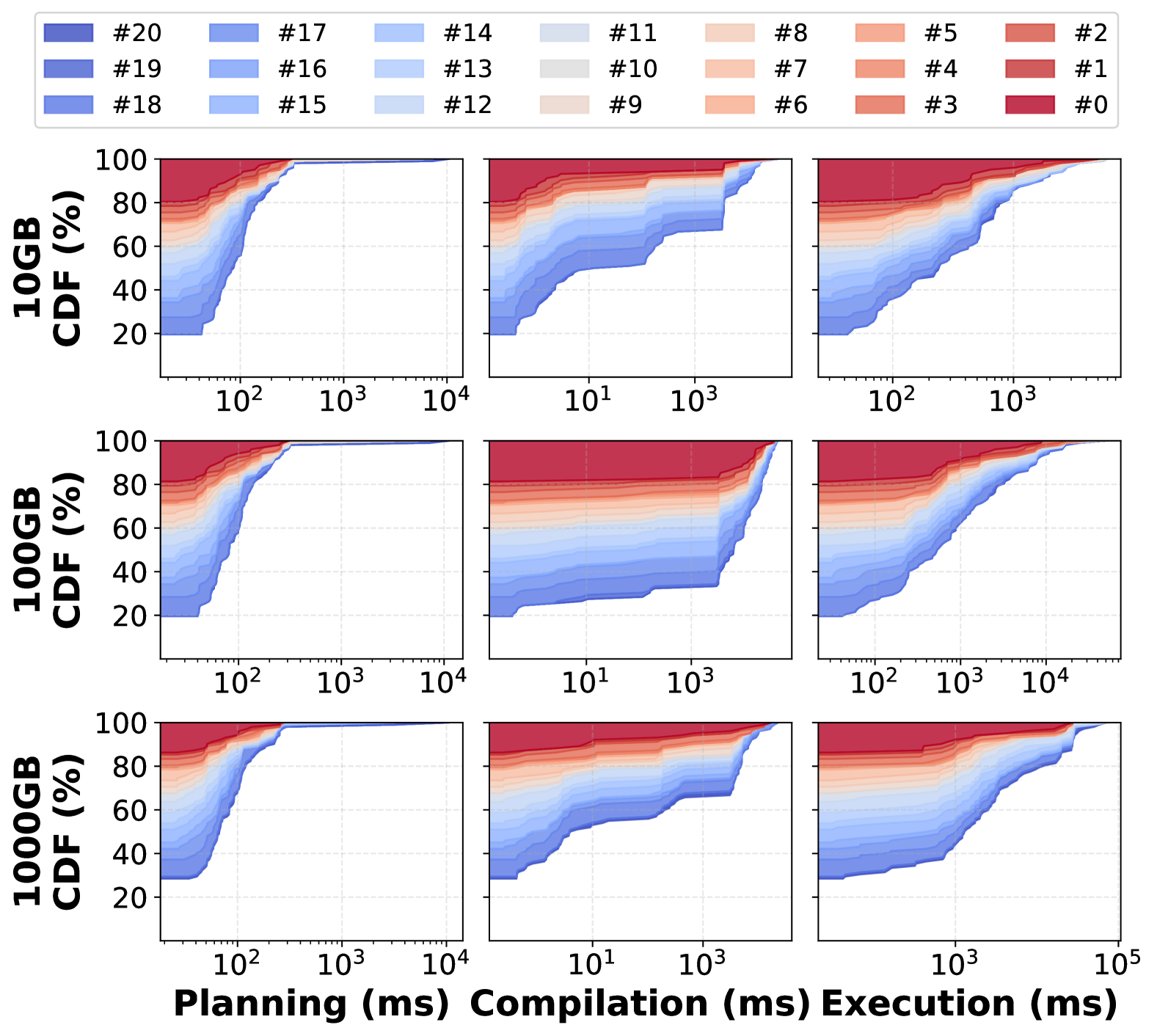
Figure 10. SpeQL overlaps query processing and user typing. "#i" represents the cumulative time since the last i lines of code are revealed.

Fig. 8 shows a breakdown of SpeQL’s overhead. We observe that the dominant factor is the LLM invocation time. The second-largest contributor is the timeout values of long-running queries, which arise due to the assumption that user input is arbitrarily slow. However, in practice, users will likely cancel these queries by pressing double ENTERs. Notably, the overhead decreases as users refine their queries, eventually dropping to near zero, as expected. At the end of §5.3.2, we show SpeQL’s cost in dollars as it was used by humans.

We show the LLM inference overhead, as depicted in Fig. 9. Although the inference time is dominant, we expect it to reduce with rapid advancements in the prompting and fine tuning of LLMs.

We further measure the overhead of the successfully created temporary tables that are directly or indirectly referenced by the final query, as illustrated in Fig. 10. We observe that SpeQL effectively distributes the overhead across the user’s thinking and typing phases. For instance, on the 100GB and 1000GB datasets, while the P90 total execution times are 7.72 seconds and 27.23 seconds, respectively, only 0.54 seconds and 1.58 seconds are incurred after the final five lines of the query are revealed, ensuring minimal perceived latency. Additionally, we observe materializing CTE and subquery results incurs reasonable overhead. On the TPC-DS 10GB dataset, only 15 out of 103 queries have an execution time exceeding 1 second, with a P90 value of 1.73 seconds — just 2.75$\times$ the baseline. For the 100GB and 1000GB datasets, while execution times increase, the overhead remains consistent with non-speculative execution. The P90 values for these datasets are 7.72 seconds and 27.23 seconds, corresponding to 2.02$\times$ and 0.49$\times$ the baseline processing times, respectively. The memory consumption is also amenable, as already shown in Table. 1. Since user experience often outweighs computational cost, and modern online analytical processing (OLAP (chaudhuri1997overview, )) databases can dynamically allocate and reclaim resources as needed, attributing to the shared, elastic, and serverless architecture, the overhead can be a worthwhile investment.

5.3. Utility/user study

5.3.1. Methodology

To add more real-world values, we conduct a utility/user study. The human involvement helps figure out three questions: (1) Can the query processing time really overlap with user’s typing time, so that SpeQL has adequate time to create temporary tables? (2) Is the LLM-based debugging logic (i.e., the speculator) necessary, without which it is nearly impossible to get a executable SQL query during editing? (3) Is SpeQL effective and efficient enough to improve users’ productivity and experience? To do this, we recruited participants to complete a 60-minute questionnaire. They were instructed to connect to our server located in Utah, which further communicates with Azure OpenAI API services in the US and a Redshift endpoint (with TPC-DS (tpcds, ) 100GB data) in Virginia.

The questionnaire includes two parts. The first part measures the utility, where we create two data analysis tasks (Q1 and Q2, as described in §5.3.2), based on the 100 GB TPC-DS dataset. We asked participants to write SQL and finish the two tasks as quickly as possible, during which we recorded their input behavior, task completion time and query latency. To compare the utility improvement, participants were randomly assigned to two groups, A and B, without their knowledge: For group A, we instructed them to learn SpeQL before showing the tasks; For group B, we only informed them that we want to record their input behavior but did not introduce SpeQL. Both groups were given five minutes to run example SQL queries and recall SQL rules to familiarize themselves with the testbed. We applied the Mann-Whitney U test to determine whether SpeQL significantly reduced task completion time, using a predefined significance level of $\alpha=0.05$, and used Cliff’s Delta to quantify the effective size.

The second part measures the usability, where participants fill in a standard system usability scale (SUS (brooke1996sus, )) tablet and leave open-ended comments on SpeQL according to their subjective experiences. Before rating the scores, group B participants undergo a debriefing session and are instructed to learn SpeQL and use it to finish the two utility tasks again.

Participants. We recruited 24 participants (12 male, 12 female) from the United States and China using email and personal contacts. All participants were allowed, but not mandated, to use their preferred AI inline completion tools, but natural language to SQL (kim2020natural, ) tools were forbidden. Participants covered diverse SQL expertise. They received monetary compensation for their time.

Data cleaning. For Q1, four participants (group A: 2, group B: 2) abandoned after multiple failed attempts, while one participant (group A) encountered a system crash during Q1, so we removed their Q1 time; For Q2, two participants (group A: 1, group B: 1) abandoned after multiple failed attempts, so we removed their Q2 time. Despite these exclusions, all participants filled the system usability scale, and their subjective evaluations were retained.

5.3.2. Utility study

We design two questions for participants that necessitate interacting with the data to derive the correct answers. Attempting to write a single SQL query without exploring the data will result in errors due to the presence of missing (NULL) values or incomplete data. Participants were told to only consider eight columns.

Q1. ”For different physical stores recorded in 2001, what is the highest annual revenue? Note, if you find the answer is close to $1.11\times 10^{9}$ USD, you may probably make a common mistake.”

General querying pattern for Q1. Nearly all participants initially listed the revenue for each store key without verifying whether the keys corresponded to valid stores, as anticipated. This led them to produce incorrect answers. Participants had to independently debug their queries to filter out invalid store keys (by checking an additional ss_store_sk column, or including an ss_store_key IS NOT NULL condition) before arriving at the correct result.

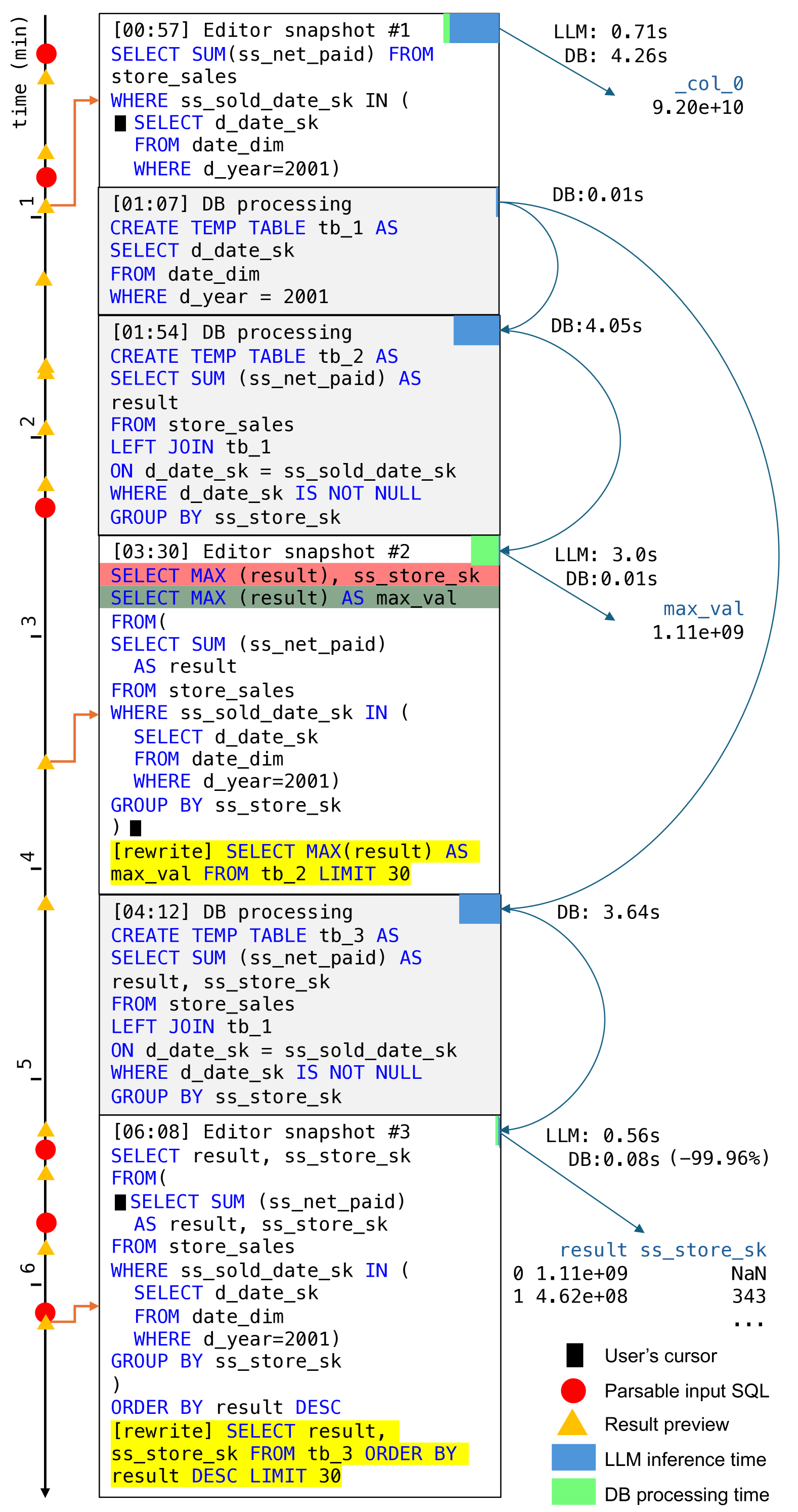
Figure 11. Case Study. Blue arrows show dependencies.

Case study for Q1. We showcase a data point from Q1 to illustrate SpeQL’s workflow and how it helps reduce latency, as shown in Fig. 11. The participant is a computer science PhD student with prior experience in a database course during undergraduate studies. Based on our records, they completed the task in approximately six minutes, which includes time spent thinking, typing, and debugging. From their input behavior, we derive three key observations, which are also observed in other participants: (1) The query processing time can fully overlap with the typing time. While typing, SpeQL created temporary tables quite early, specifically, tb_1, tb_2 and tb_3 were created at 01:07, 01:54 and 04:12, respectively. This indicates that there would be sufficient time to generate temporary tables in advance. (2) LLM is necessary for efficient speculative query execution. When typing, the user’s inputs were syntactically correct at only six moments (00:06, 00:52, 02:14, 05:18, 05:45, and 06:03, the red circles), five of which occurred between the first (because the query is short) and last (because the participant had already debugged for a while) minute. We analyzed their behavior and found that they forgot to include one column in the GROUP BY clause (snapshot #2). These syntax errors were common among participants when constructing their SQL queries. (3) SpeQL is an effective tool for reducing query latency. As we observed, the participant had a tendency to first execute simple SQL queries, inspect their results, and then integrate these into a larger, more complex logic. This behavior reinforces the feasibility of SpeQL materializing the results of subqueries, such as tb_1 in snapshot #1, tb_2 in snapshot #2, and tb_3 in snapshot #3. With the help of the precomputed temporary tables, SpeQL completed the final query within 0.08 seconds, which is $289\times$ faster than the baseline (simply pasting and running the query in Redshift query editor takes 23.1 seconds). Furthermore, during the editing process, SpeQL provided nine previews (the orange triangles), six of which occurred between the first and fifth minute when the SQL typically contained syntax errors. The participant later acknowledged that these previews were highly helpful for debugging and refining the SQL query.

Q2. ”Calculate the total revenue for physical stores (sum of all ss_net_paid in the store_sales table) for each year from 2000 to 2003. Analyze the reasons for the changes in total revenue in 2003.”

General querying pattern for Q2. To address this question, participants first computed the total revenue across different years. They quickly observed that revenue in 2003 was significantly lower. By crafting more advanced queries, possibly after checking quantities and number of stores, they eventually discovered that the data for 2003 was truncated starting from January and the dataset is incomplete.

Case study for Q2. One particularly interesting finding in Q2 is SpeQL helps users stop querying earlier once they find the desired information. For instance, to calculate the total revenue, participants in group B typically wrote the following query (with result in the comment):

SELECT d_year, SUM (ss_net_paid) FROM store_sales JOIN
date_dim ON ss_sold_date_sk = d_date_sk
WHERE d_year >= 2000 AND d_year <= 2003
GROUP BY d_year ORDER BY d_year;
/* 2000: 9e10; 2001: 9e10; 2002: 9e10; 2003: 1e9 */

This query is entirely correct, as it applies strict filtering conditions to eliminate out-of-bounds data. However, participants often needed more time to write such a query, and most of them remained confused about the revenue drop for a while. In contrast, we observed that participants in group A derived the same insights much faster. They typed (with grey code generated by LLMs):

SELECT d_year, SUM (ss_net_paid) FROM store_sales JOIN
date_dim  ON ss_sold_date_sk = d_date_sk GROUP BY d_year
/* 2002: 9e10; 2003: 1e9; 1998: 9e10; 1999: 9e10; 2000: 9e10; 2001: 9e10 */

The preview included additional years of revenue that users did not initially intend to request. However, it unexpectedly helped them identify the time boundary: 2003 was the last year in the dataset. As a result, we observed that participants in group B quickly realized the data was incomplete. We did not anticipate this benefit when designing the tasks.

Statistics. (1) Fig. 12 (a) presents the query latency measured immediately after group A participants composed and finalized the runnable queries in their editor. In contrast, the baseline represents the query latency observed when the queries were directly issued without any preprocessing. We find that SpeQL significantly and effectively reduces latency, with a significance level of $p<0.001$, and Cliff’s Delta $\delta=-1.0$ for Q1, and $p<0.001,\delta=-0.778$ for Q2. (2) Figure 12 (b) depicts the overall duration of Q1, where we observed neither significance ($p=0.775$) nor difference ($\delta=0.089$) between the two groups. We guess that this could be a limitation of our utility study setup — we should have created a warm-up task Q0 to help them get accustomed to SpeQL and the dataset. (3) Figure 12 (c) presents the overall duration of Q2, demonstrating that SpeQL significantly ($p=0.025$) and effectively ($\delta=-0.570$) improves participants’ task completion speed. We observe SpeQL’s previews provide additional information while they are typing, which helps them quickly eliminate unlikely exploration directions. (4) As a cost, each group A participant spent about $1.5 on database usage and $0.5 on LLM API (not shown in the figure), which is affordable and can be further optimized.

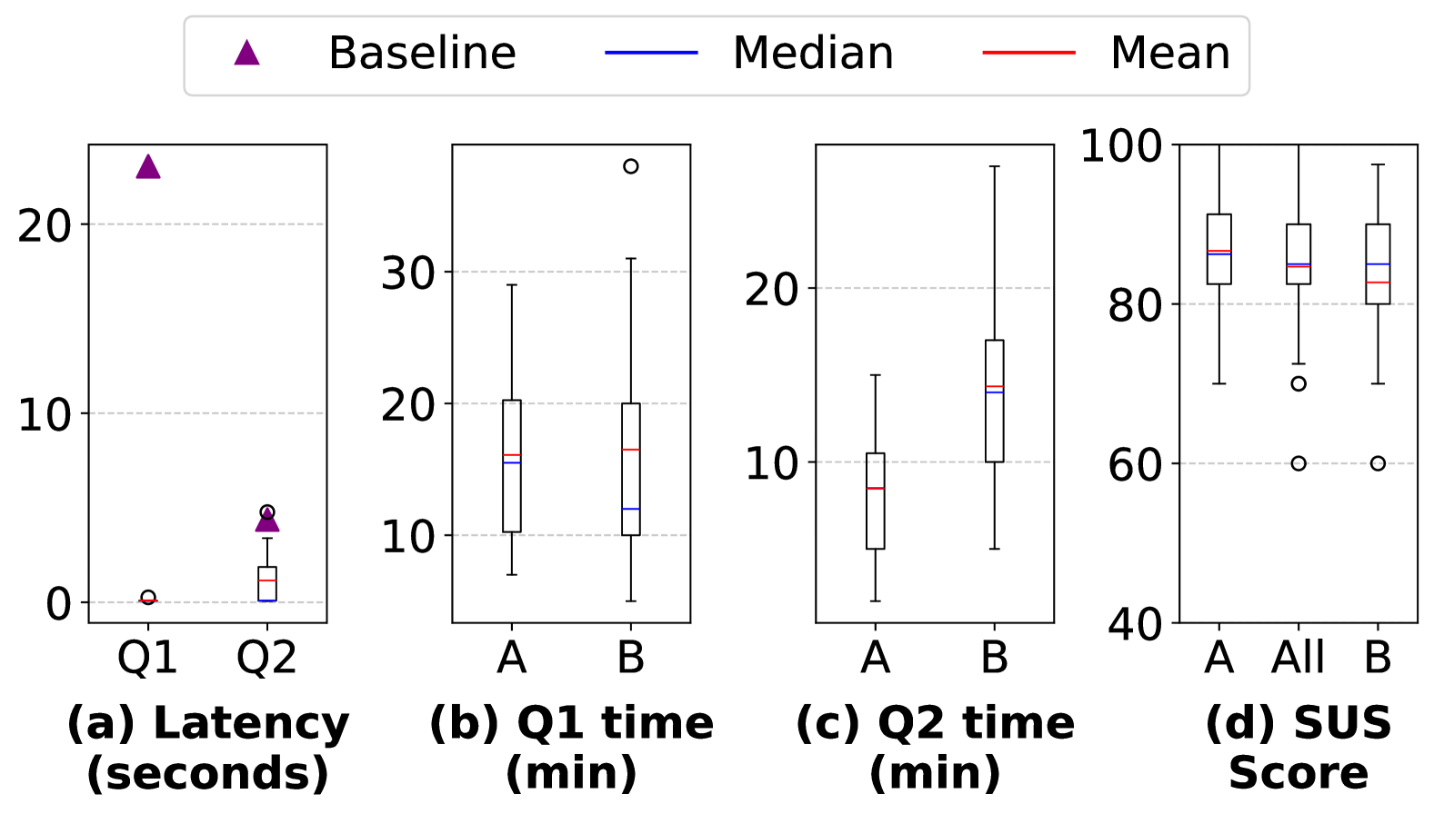
Figure 12. Utilily/user study. In (a), the boxes represent SpeQL’s latency while the purple triangles represent the baseline’s. In (b), (c), (d), the boxes in group A are SpeQL’s result while that in group B are the baseline’s.

5.3.3. User study

This section captures users’ subjective perceptions of SpeQL’s usability and utility. The System Usability Scale (SUS (brooke1996sus, )) confirms the high usability of SpeQL. In the SUS questionnaire, participants were encouraged to focus primarily on the system’s functionality and efficiency, rather than the user interface design, while responding to ten subjective statements to gauge their perception on SpeQL. The results are shown in Fig. 12, where the SUS score of the two groups does not present significance ($p=0.771$) or difference ($\delta=-0.076$), indicating that both groups would want to use SpeQL. SpeQL achieved an excellent SUS score of 85.3, including a learnability score of 85.8 and usability score of 83.3. This score outperforms approximately 95% of systems, as illustrated in Fig. 12 (d), indicating that users are happy to use, and are willing to promote SpeQL in production. Specifically, 58.3% of participants strongly agreed that they would frequently use SpeQL when writing SQL queries, and 79.2% of participants strongly agreed that most people can learn SpeQL very quickly.

The open-ended survey highlights significant productivity gains and areas for future improvement of SpeQL. We gathered subjective evaluations from participants regarding their experience with SpeQL. Notably, 87.5% of participants agreed that SpeQL improves their productivity. Most respondents acknowledged that SpeQL simplifies the process of writing and debugging SQL, even when using existing inline code assistants such as GitHub Copilot (chen2021evaluating, ). Several participants highlighted that the intermediate previews transformed their workflow: Instead of focusing solely on code, they interacted with data more frequently and became more confident, especially students and learners. More than 33.3% of participants emphasized the potential of integrating SpeQL into commercial SQL IDEs/BIs with an enhanced user interface. Suggested features included “submit” buttons, automatic plotting, and next-step query recommendations. Participants also agreed that these enhancements are orthogonal to SpeQL’s core functionality. At the same time, some participants expressed concerns regarding the applicability of SpeQL to more complex SQL queries (we kept the questions simple to encourage participation), and the uncertainty in LLM-generated predictions and preview pop-ups were potential distractions for users, which require further improvements.

6. Related Work

Speculative query processing (polyzotis2003speculative, ) was first introduced in 2003, revealing the opportunity to overlap query execution with user input. It had the foresight to propose the use of machine learning to predict user behavior. However, the work had limitations since it was in 2003, especially for data exploration scenarios. For example, it relied on predefined query structures, where relations were represented in a tabular format. Users were required to construct queries by manually placing projection indicators and selection predicates on the corresponding fields. However, the assumption falls short in ad-hoc queries, where users often compose complex and structurally diverse SQL queries (hatami2020understanding, ). Such queries may contain syntax errors, rendering them unrunnable, or may take significantly longer to compile than to execute, even with Just-In-Time (JIT (viglas2014just, )) compilation. Recent work on incremental query processing has been proposed, primarily targeting interpreted languages (xin2021enhancing, ) or already well-formed queries (sioulas2021accelerating, ). In contrast, SpeQL harnesses LLMs to overcome these constraints, providing a more flexible and intelligent approach to speculative ad-hoc querying.

Query optimization (jarke1984query, ) SpeQL leverages many query optimization techniques originally developed for self-tuning systems  (chaudhuri2007self, ) that dynamically adapt to historical workload changes, for example result caches, query compilation/plan caches (armenatzoglou2022amazon, ; ibmplancache, ), and materialized views (gupta1995maintenance, ) (akin to SpeQL’s temporary tables). To materialize partial results and reuse them, SpeQL uses common subexpression elimination (zaharioudakis2000answering, ), view selection (chirkova2002formal, ), and view matching (halevy2001answering, ). SpeQL leverages approximate/progressive query execution (garofalakis2001approximate, ; hellerstein2000informix, ) to improve the interactivity of data analysis workflows (hellerstein1999interactive, ), by advising the database to provide either approximate (e.g., sampling 5% rows on large tables) or partial (e.g., limiting to 30 rows to the preview query) results. SpeQL uses these techniques to improve single-user scenarios and proactively begins computation even before the SQL query is formally issued.

Natural language to SQL (NL2SQL, a.k.a. Text-to-SQL (kim2020natural, )) is an active research area that is similar to, but orthogonal to, SpeQL. NL2SQL converts natural language questions into SQL queries and lowers the barrier to using SQL databases. It deals with the challenges of the ambiguity of natural language, the complexity of database schemas, and issues with dirty data (e.g., missing or duplicate values) that make it difficult to construct correct and efficient SQL queries. In contrast, SpeQL converts from SQL to speculative queries to reduce response latency. For recent advancements in NL2SQL, we refer readers to a survey (liu2024survey, ).

7. Limitations and Future work

SpeQL has several limitations and offers new avenues for database optimization. For instance, with each user input, SpeQL must decide whether to cancel prior jobs or wait. This decision becomes even harder in multi-tenant settings. Selecting which temporary tables to create and which existing ones to use for a new query has parallels with materialized view selection (mami2012survey, ). Addressing this in the context of speculative ad-hoc querying requires deeper integration with cardinality estimators. Another challenge is that LLM hallucinations can create wasteful queries and distract users. This issue may be reduced with better prompts, model fine-tuning and UX design.

Integration with more IDEs and Business Intelligence (BI (negash2008business, )) tools, and insights from the field of Human Computer Interaction (HCI) can improve user experience. Future work could develop tools that enable analysts to seamlessly view plots, analytical suggestions and query recommendations on the fly. Future work can adapt SpeQL to speculate not only on humans generating queries, but also NL2SQL and Retrieval-Augmented Generation (lewis2020retrieval, ) (RAG) systems.

8. Conclusion

This paper proposes speculative ad-hoc querying, unlocking new query optimization opportunities by leveraging the time spent on SQL query construction, and presents SpeQL, a powerful AI-coding assistance facilitating instantaneous interaction between humans and data. Our experiments show that SpeQL reduces query latency from tens of seconds to milliseconds with reasonable overhead, even on datasets of hundreds of gigabytes, and its feature to peek intermediate results significantly and effectively improves user’s productivity for interactive data exploration.

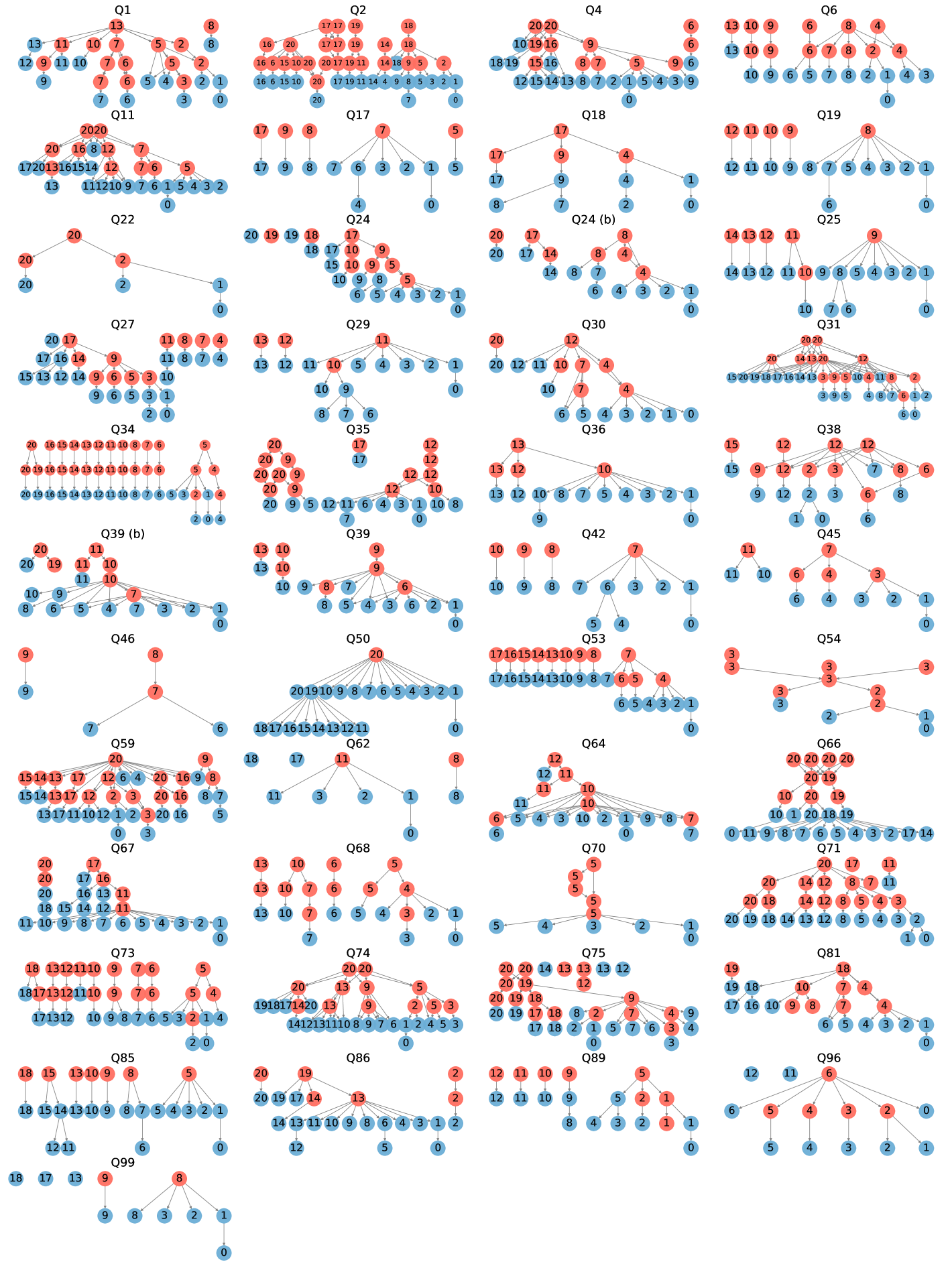
Figure 13. Tree-like DAGs for TPCDS 100GB.

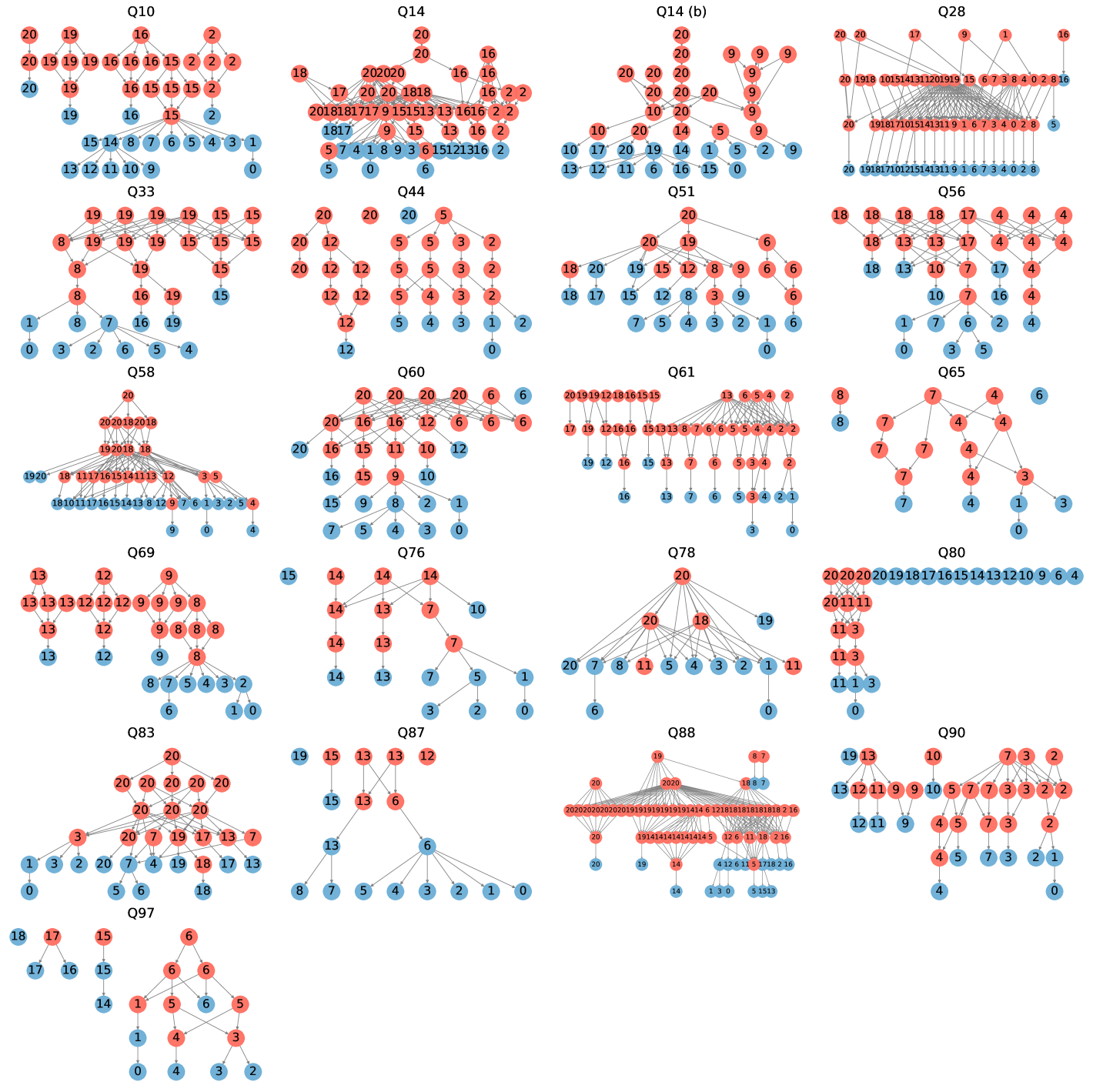
Figure 14. Mesh-like DAGs for TPCDS 100GB.

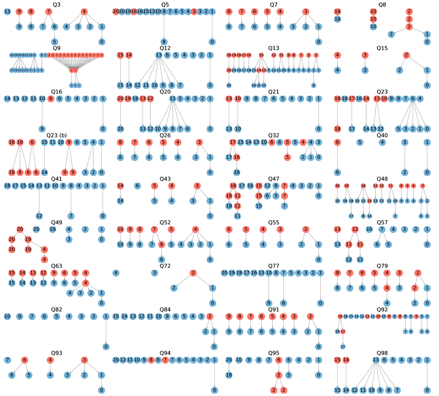
Figure 15. Linear-like DAGs for TPCDS 100GB.

- [1] James Phillips. Over 5 million subscribers are embracing power bi for modern business intelligence. Available at: https://powerbi.microsoft.com/fr-fr/blog/over-5-million-subscribers-are-embracing-power-bi-for-modern-business-intelligence/.
- [2] Amazon Web Services. Redshift powers analytical workloads for fortune 500 companies, startups, and everything in between. Available at: https://aws.amazon.com/redshift/customer-success/?awsf.customer-references-location=*all&awsf.customer-references-segment=*all&awsf.customer-references-industry=*all.
- [3] Zhicheng Liu and Jeffrey Heer. The effects of interactive latency on exploratory visual analysis. IEEE transactions on visualization and computer graphics, 20(12):2122–2131, 2014.
- [4] Jeff Shute, Shannon Bales, Matthew Brown, Jean-Daniel Browne, Brandon Dolphin, Romit Kudtarkar, Andrey Litvinov, Jingchi Ma, John Morcos, Michael Shen, et al. Sql has problems. we can fix them: Pipe syntax in sql. Proceedings of the VLDB Endowment, 17(12):4051–4063, 2024.
- [5] Raghunath Othayoth Nambiar and Meikel Poess. The making of tpc-ds. VLDB ’06, page 1049–1058. VLDB Endowment, 2006.
- [6] Nikos Armenatzoglou, Sanuj Basu, Naga Bhanoori, Mengchu Cai, Naresh Chainani, Kiran Chinta, Venkatraman Govindaraju, Todd J Green, Monish Gupta, Sebastian Hillig, et al. Amazon redshift re-invented. In Proceedings of the 2022 International Conference on Management of Data, pages 2205–2217, 2022.
- [7] IBM. Query plan caching (entity sql). Available at: https://www.ibm.com/docs/en/i/7.4?topic=overview-plan-cache.
- [8] Matthijs Douze, Alexandr Guzhva, Chengqi Deng, Jeff Johnson, Gergely Szilvasy, Pierre-Emmanuel Mazaré, Maria Lomeli, Lucas Hosseini, and Hervé Jégou. The faiss library. arXiv preprint arXiv:2401.08281, 2024.
- [9] Xinyun Chen, Maxwell Lin, Nathanael Schärli, and Denny Zhou. Teaching large language models to self-debug. arXiv preprint arXiv:2304.05128, 2023.
- [10] Toby Mao. Sqlglot: Python sql parser and transpiler. Available at: https://github.com/tobymao/sqlglot.
- [11] Alon Y Halevy. Answering queries using views: A survey. The VLDB Journal, 10:270–294, 2001.
- [12] Minos N Garofalakis and Phillip B Gibbons. Approximate query processing: Taming the terabytes. In VLDB, volume 10, pages 645927–672356, 2001.
- [13] Ashish Gupta, Inderpal Singh Mumick, et al. Maintenance of materialized views: Problems, techniques, and applications. IEEE Data Eng. Bull., 18(2):3–18, 1995.
- [14] Itzik Ben-Gan and Tom Moreau. Temporary tables. In Advanced Transact-SQL for SQL Server 2000, pages 435–458. Springer, 2000.
- [15] Raghu Ramakrishnan and Johannes Gehrke. Database management systems. McGraw-Hill, Inc., 2002.
- [16] Solomon Negash and Paul Gray. Business intelligence. Handbook on decision support systems 2, pages 175–193, 2008.
- [17] Gloria Chatzopoulou, Magdalini Eirinaki, and Neoklis Polyzotis. Query recommendations for interactive database exploration. In Scientific and Statistical Database Management: 21st International Conference, SSDBM 2009 New Orleans, LA, USA, June 2-4, 2009 Proceedings 21, pages 3–18. Springer, 2009.
- [18] Surajit Chaudhuri and Umeshwar Dayal. An overview of data warehousing and olap technology. ACM Sigmod record, 26(1):65–74, 1997.
- [19] Amazon Web Services. Amazon redshift pricing. Available at: https://aws.amazon.com/redshift/pricing/?nc1=h_ls.
- [20] Amazon Web Services. Tpc-ds benchmark data (test product). Available at: https://aws.amazon.com/marketplace/pp/prodview-iopazp7irqk6s.
- [21] Aixin Liu, Bei Feng, Bing Xue, Bingxuan Wang, Bochao Wu, Chengda Lu, Chenggang Zhao, Chengqi Deng, Chenyu Zhang, Chong Ruan, et al. Deepseek-v3 technical report. arXiv preprint arXiv:2412.19437, 2024.
- [22] Daya Guo, Dejian Yang, Haowei Zhang, Junxiao Song, Ruoyu Zhang, Runxin Xu, Qihao Zhu, Shirong Ma, Peiyi Wang, Xiao Bi, et al. Deepseek-r1: Incentivizing reasoning capability in llms via reinforcement learning. arXiv preprint arXiv:2501.12948, 2025.
- [23] Joseph M Hellerstein, Ron Avnur, and Vijayshankar Raman. Informix under control: Online query processing. Data Mining and Knowledge Discovery, 4:281–314, 2000.
- [24] Meikel Poess and Chris Floyd. New tpc benchmarks for decision support and web commerce. ACM Sigmod Record, 29(4):64–71, 2000.
- [25] Jordan Tigani. Big data is dead. Available at: https://motherduck.com/blog/big-data-is-dead/.
- [26] John Brooke et al. Sus-a quick and dirty usability scale. Usability evaluation in industry, 189(194):4–7, 1996.
- [27] Hyeonji Kim, Byeong-Hoon So, Wook-Shin Han, and Hongrae Lee. Natural language to sql: Where are we today? Proceedings of the VLDB Endowment, 13(10):1737–1750, 2020.
- [28] Mark Chen, Jerry Tworek, Heewoo Jun, Qiming Yuan, Henrique Ponde De Oliveira Pinto, Jared Kaplan, Harri Edwards, Yuri Burda, Nicholas Joseph, Greg Brockman, et al. Evaluating large language models trained on code. arXiv preprint arXiv:2107.03374, 2021.
- [29] Neoklis Polyzotis and Yannis E Ioannidis. Speculative query processing. In CIDR. Citeseer, 2003.
- [30] Zahra Hatami and Peter Wolcott. Understanding students’ identification and use of patterns while writing sql queries. In Proceedings of the 21st Annual Conference on Information Technology Education, pages 20–25, 2020.
- [31] Stratis D Viglas. Just-in-time compilation for sql query processing. In 2014 IEEE 30th International Conference on Data Engineering, pages 1298–1301. IEEE, 2014.
- [32] Doris Xin, Devin Petersohn, Dixin Tang, Yifan Wu, Joseph E Gonzalez, Joseph M Hellerstein, Anthony D Joseph, and Aditya G Parameswaran. Enhancing the interactivity of dataframe queries by leveraging think time. arXiv preprint arXiv:2103.02145, 2021.
- [33] Panagiotis Sioulas, Viktor Sanca, Ioannis Mytilinis, and Anastasia Ailamaki. Accelerating complex analytics using speculation. In CIDR, 2021.
- [34] Matthias Jarke and Jurgen Koch. Query optimization in database systems. ACM Computing surveys (CsUR), 16(2):111–152, 1984.
- [35] Surajit Chaudhuri and Vivek Narasayya. Self-tuning database systems: a decade of progress. In Proceedings of the 33rd international conference on Very large data bases, pages 3–14, 2007.
- [36] Markos Zaharioudakis, Roberta Cochrane, George Lapis, Hamid Pirahesh, and Monica Urata. Answering complex sql queries using automatic summary tables. In Proceedings of the 2000 ACM SIGMOD international conference on Management of data, pages 105–116, 2000.
- [37] Rada Chirkova, Alon Y Halevy, and Dan Suciu. A formal perspective on the view selection problem. The VLDB Journal, 11:216–237, 2002.
- [38] Joseph M Hellerstein, Ron Avnur, Andy Chou, Christian Hidber, Chris Olston, Vijayshankar Raman, Tali Roth, and Peter J Haas. Interactive data analysis: The control project. Computer, 32(8):51–59, 1999.
- [39] Xinyu Liu, Shuyu Shen, Boyan Li, Peixian Ma, Runzhi Jiang, Yuxin Zhang, Ju Fan, Guoliang Li, Nan Tang, and Yuyu Luo. A survey of nl2sql with large language models: Where are we, and where are we going? arXiv preprint arXiv:2408.05109, 2024.
- [40] Imene Mami and Zohra Bellahsene. A survey of view selection methods. Acm Sigmod Record, 41(1):20–29, 2012.
- [41] Patrick Lewis, Ethan Perez, Aleksandra Piktus, Fabio Petroni, Vladimir Karpukhin, Naman Goyal, Heinrich Küttler, Mike Lewis, Wen-tau Yih, Tim Rocktäschel, et al. Retrieval-augmented generation for knowledge-intensive nlp tasks. Advances in Neural Information Processing Systems, 33:9459–9474, 2020.