Possible Explanation of $F_{2}^{n}/F_{2}^{p}$ at Large $x$ Using Quantum Statistical Mechanics

Abstract

The ratio of the neutron to proton structure functions, $F^{n}_{2}(x)/F^{p}_{2}(x)$, is expected to approach 1/4 as $x\to 1$, based on the assumption that $d(x)/u(x)$ vanishes as $x\to 1$. This expectation is in striking disagreement with a recent measurement by the Marathon experiment of the scattering of electrons off the mirror nuclei ³H and ³He, showing that $F^{n}_{2}(x)/F^{p}_{2}(x)$ is larger than 1/4 for $x\rightarrow 1$. We have examined the consequences of the Pauli Exclusion Principle for the parton distributions in the nucleon when the partons are described by quantum statistical mechanics. We find that the recent experimental result on the $F^{n}_{2}(x)/F^{p}_{2}(x)$ over the broad range of $x$ can be well described by the quantum statistical approach.

Deep Inelastic Scattering (DIS) of electrons from nucleons, and the subsequent extraction of the structure functions, led to the discovery of the quarks and antiquarks substructure of the nucleons. It also provided a solid basis for establishing Quantum Chromodynamics (QCD) as the correct theory for the strong interaction SM1 ; SM2 ; SM3 ; SM4 ; SM5 ; SM6 ; SM7 ; SM8 ; SM9 .

The differential cross sections for DIS are expressed in terms of the nucleon structure functions, $F_{1}$ and $F_{2}$ :

$$\frac{d^{2}\sigma}{d\Omega dE^{{}^{\prime}}}=\sigma_{M}\left[\frac{F_{2}(\nu,Q^{2})}{\nu}+2\frac{F_{1}(\nu,Q^{2})}{M}\tan^{2}\left(\frac{\theta}{2}\right)\right],$$ (1)

in which $\sigma_{M}$ is the Mott cross section, $E^{{}^{\prime}}$ and $\theta$ are the energy and polar angle of the scattered electron, $\nu=E-E^{{}^{\prime}}$ where $E$ is the incident electron energy, $Q^{2}=4EE^{{}^{\prime}}\sin^{2}\theta/2$ is the negative of the momentum transfer squared, and $M$ is the nucleon mass.

In the quark-parton model, DIS is represented as scattering of electrons from point-like constituents, carrying the momentum fraction, $x$, of the nucleon. In the infinite momentum scaling limit when $\nu\rightarrow\infty,Q^{2}\rightarrow\infty$, $0\leq(x\equiv Q^{2}/2M\nu)\leq 1$, the structure function $F_{2}$ becomes

$$F_{2}(x)=x\Sigma_{i}e_{i}^{2}f_{i}(x),$$ (2)

where $f_{i}(x)dx$ is the probability that a parton of type $i$ carries momentum in the range between $x$ and $x+dx$, and the sum in Eq. (2) runs over all parton types.

We consider the up ($u$), down ($d$), and strange ($s$) quarks in the proton and define $U(x)\equiv u(x)+\bar{u}(x)$, $D(x)\equiv d(x)+\bar{d}(x)$ and $S(x)\equiv s(x)+\bar{s}(x)$. With these notations, together with the assumption of isospin symmetry for the nucleon PDFs, we have

$$F_{2}^{p}(x)=x\left[\frac{4}{9}U(x)+\frac{1}{9}D(x)+\frac{1}{9}S(x)\right]$$ (3)

and

$$F_{2}^{n}(x)=x\left[\frac{1}{9}U(x)+\frac{4}{9}D(x)+\frac{1}{9}S(x)\right]$$ (4)

Because all parton distribution functions are non-negative we deduce from Eqs. (3) and (4) that the $F^{n}_{2}(x)/F^{p}_{2}(x)$ ratio, $r(x)$, is bounded at all $x$ by

$$1/4\leq\left(r(x)\equiv\frac{F_{2}^{n}(x)}{F_{2}^{p}(x)}\right)\leq 4$$ (5)

which is known as the Nachtmann inequality Nachtmann .

The earliest DIS experiments at SLAC GottfriedExperiment confirmed the Nachtmann inequality and, more specifically, discovered that, for $x\rightarrow 0$, $r$ is approximately unity, whereas for $x\rightarrow 1$, with much larger errors, it was thought that $r$ might asymptotically approach $1/4$. However, the uncertainties of the nuclear effects for the deuteron nucleus have raised some concerns on the validity of the extraction of $r(x)$ at large $x$ Whitlow92 ; Thomas96 . New measurements which would minimize the nuclear effects were proposed for a more reliable determination of $r(x)$ at large $x$ Afnan00 .

Recently, the Marathon experiment Abrams , performed by the Jefferson Laboratory Hall A Tritium Collaboration, has measured the DIS of electrons from the mirror nuclei ³H and ³He in order to cleanly separate the proton and neutron structure functions. The measured values of $r(x)$ cover a broad range of $x$, from $x=0.19$ up to $x=0.83$. As shown in Fig. 1, the $F^{n}_{2}(x)/F^{p}_{2}(x)$ from the Marathon experiment exhibit an intriguing $x$ dependence. At intermediate $x$ region ($0.19<x<0.5$), $F^{n}_{2}(x)/F^{p}_{2}(x)$ falls roughly linearly with $x$, while for the large $x$ region, $F^{n}_{2}(x)/F^{p}_{2}(x)$ falls off more slowly with $x$, approaching a constant value of $\sim 0.45$ at the highest values of $x$.

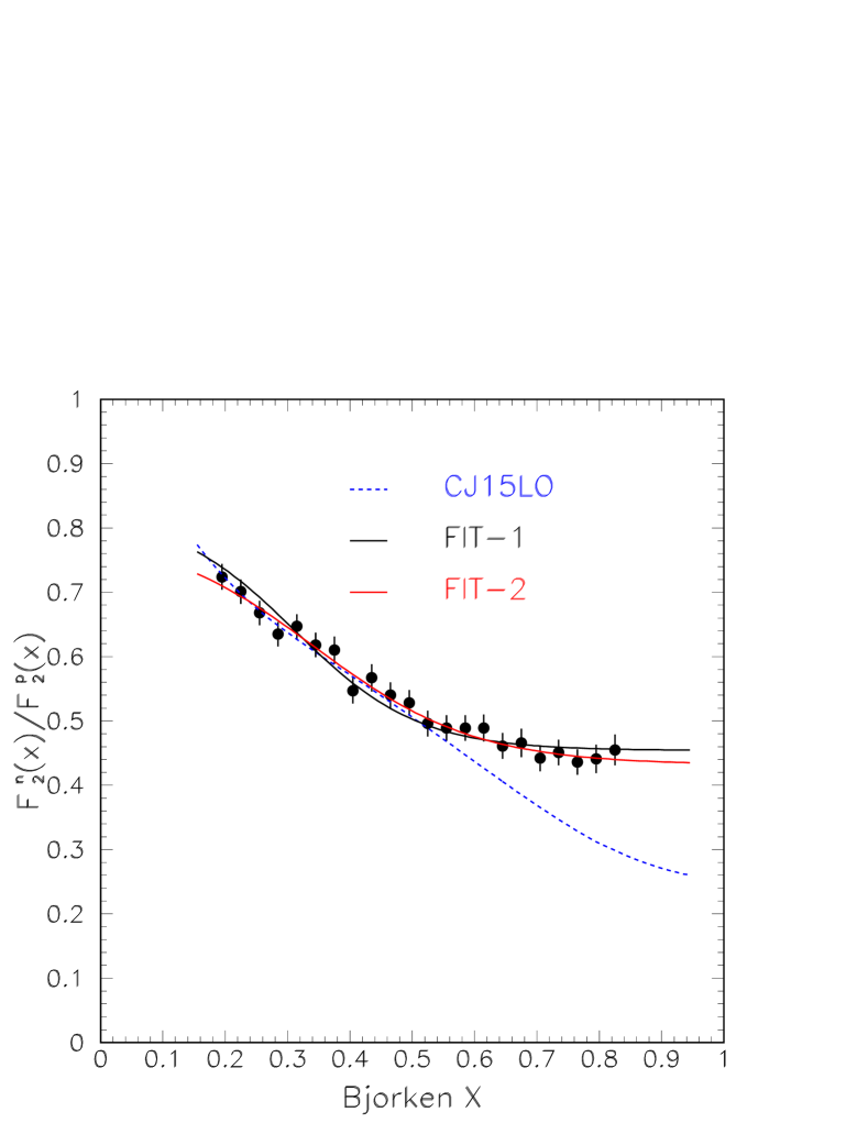
Figure 1: Comparison of the Marathon data with calculations. The dashed curve is obtained using the CJ15LO proton PDFs CJ . The solid curves are obtained from the statistical model using the two sets of parameters listed in Table I: $\bar{x}=0.099$ (black) and $\bar{x}=0.128$ (red), respectively.

As discussed in the Marathon paper, the observed $x$ dependence for $F^{n}_{2}(x)/F^{p}_{2}(x)$ is at variance with the prediction of the CTEQ-JLab (CJ) Collaboration, based on a global fit of existing data using the conventional functional forms for describing the parton distributions CJ . As shown by the dashed curve in Fig. 1, the calculated $F^{n}_{2}(x)/F^{p}_{2}(x)$ using the CJ15LO proton PDFs falls off with $x$, approaching a value of 1/4 as $x\to 1$, in disagreement with the Marathon data.

The Marathon results on $F^{n}_{2}(x)/F^{p}_{2}(x)$ in a broad region in $x$ up to the largest value $x=0.83$ have inspired several recent papers to address various aspects of the data Va ; Ha ; Ab ; Li ; Gr ; Ar ; Ac ; Ar1 ; Al ; Ro , including the off-shell contributions Ha and the EMC effect Ab . In this Letter, we show that the Marathon data on $F^{n}_{2}(x)/F^{p}_{2}(x)$ can be well described by an approach based on the quantum statistical mechanics. The good agreement between the Marathon data and the statistical approach lends further support for the validity of this approach in depicting the partonic structures of hadrons.

We first briefly discuss the salient features of the quantum statistical approach in depicting the dynamics of partons inside the nucleons. The rule of the Pauli Exclusion Principle NiegawaSasaki ; FieldFeynman implies quantum statistical parton distributions, namely Fermi-Dirac type for the quarks and antiquarks and Bose-Einstein type for the gluons. In 2002, Bourrely, Buccella and Soffer BBS proposed the following distributions at the initial scale, $Q_{0}=2$ GeV/c for the quarks and antiquarks ($q(x),\bar{q}(x)$), and the gluons ($G(x)$), on the basis of quantum statistical mechanics:

$$xq^{h}(x) = AX_{q}^{h}x^{b}\left[\exp\frac{(x-X_{q}^{h})}{\bar{x}}+1\right]^{-1}$$ (6)

$$+ \tilde{A}x^{\tilde{b}}\left[\exp\frac{x}{\bar{x}}+1\right]^{-1}$$

and

$$x\bar{q}^{h}(x) = \bar{A}x^{\bar{b}}\left[X_{q}^{-h}(\exp\frac{(x+X_{q}^{-h})}{\bar{x}}+1)\right]^{-1}$$ (7)

$$+ \tilde{A}x^{\tilde{b}}\left[\exp\frac{x}{\bar{x}}+1\right]^{-1}$$

and

$$xG(x)=A_{G}x^{b_{G}}\left[\exp\frac{(x-X_{G})}{\bar{x}}-1\right]^{-1}.$$ (8)

In these distributions, $\bar{x}$ plays the rôle of temperature. $X_{q}^{h}$ are chemical potentials depending on the flavour ($q$ = $u$ or $d$) and the helicity ($h$). The factors $X_{q}^{h}$ in Eq. (6) and $(X_{q}^{-h})^{-1}$ in Eq. (7) were introduced in BBS to comply with the data and have been accounted for by considering the transverse degrees of freedom BBS4 . The normalization factors $A,\tilde{A},\bar{A}$ and the exponents $b,\tilde{b},\bar{b}$ are determined by fitting the data, together with the constraints of the quark number sum rule and the momentum sum rule. For the strange partons, it was assumed that $s(x)=\bar{s}(x)=(\bar{u}(x)+\bar{d}(x))/4$.

The Fermi-Dirac form for the quark and antiquark distributions are very different from the $Ax^{B}(1-x)^{C}$ form for standard parametrizations. This difference would lead naturally to different behaviors of $F^{n}_{2}(x)/F^{p}_{2}(x)$ between the statistical model and the conventional parametrization.

The equilibrium conditions with respect to the processes which lead to the DGLAP equations DGLAP imply that

$$X_{q}^{h}+X_{\bar{q}}^{-h}=0$$ (9)

and

$$X_{G}=0.$$ (10)

Equation (9) provides a natural connection between the valence and sea quark parton distributions, since the chemical potentials of the quark $q$ and antiquark $\bar{q}$ are related. It also implies that the helicities of the quark and antiquark are correlated. These intriguing correlations between quark and antiquark distributions, and between their positive and negative helicity distributions, are unique features of the quantum statistical approach and they are absent in the usual standard parametrizations of nucleon PDFs in the conventional global fits.

The values of $\bar{x}$ and $X^{h}_{q}$, found in the first paper BBS in 2002, are respectively:

$$\bar{x}=0.099;~X_{u}^{\uparrow} = 0.461;~X_{d}^{\downarrow}=0.302;$$

$$X_{u}^{\downarrow} = 0.298;~X_{d}^{\uparrow}=0.228.$$ (11)

Following the cited paper BBS , supporting confirmations were forthcoming for the quantum statistical parton distributions proposed therein. The temperature $\bar{x}$ and the quark chemical potentials were obtained, for example, in the 2015 global fit in the quantum statistical approach BS1 with $Q_{0}=1$ GeV, as follows:

$$\bar{x}=0.090;~X_{u}^{\uparrow} = 0.475;~X_{d}^{\downarrow}=0.309;$$

$$X_{u}^{\downarrow} = 0.307;~X_{d}^{\uparrow}=0.245.$$ (12)

An upgraded fit at NLO of the statistical model BS1 , which includes the Marathon data, requires the introduction of a $Q^{2}$ dependence of the dimensionless temperature whose values are given in the domain $0.0909\leq\bar{x}\leq 0.0984$ Bourr . The following values have been found for the chemical potential parameters :

$$X_{u}^{\uparrow} = 0.447;~X_{d}^{\downarrow}=0.314;$$

$$X_{u}^{\downarrow} = 0.311;~X_{d}^{\uparrow}=0.227.$$ (13)

One observes the following inequalities for the chemical potentials of the valence quarks:

$$X_{u}^{\uparrow}>X_{d}^{\downarrow}>X_{u}^{\downarrow}>X_{d}^{\uparrow}.$$ (14)

Eqs. (9) and (14) imply the following inequalities for the chemical potentials of the antiquarks:

$$X_{\bar{u}}^{\downarrow}<X_{\bar{d}}^{\uparrow}<X_{\bar{u}}^{\uparrow}<X_{\bar{d}}^{\downarrow}.$$ (15)

Eq. (15) leads to the following striking predictions of the quantum statistical approach for the flavor and spin structure of the antiquarks in the proton:

$$\bar{d}(x)>\bar{u}(x)$$ (16)

and

$$\Delta\bar{u}(x)>0>\Delta\bar{d}(x)$$ (17)

and finally

$$\Delta\bar{u}(x)-\Delta\bar{d}(x)>\bar{d}(x)-\bar{u}(x).$$ (18)

The first inequality, Eq. (16), has been confirmed by the Fermilab E866 experiment E866a ; E866b ; E866c and the SeaQuest experiment Do1 ; Do . The second inequality, Eq. (17), has been confirmed by the STAR Collaboration at RHIC on the production of charged weak bosons using polarized beams JAdam . The test of the last inequality, Eq. (18), still awaits a more precise determination of the quantity on the left-hand side.

The gluon parton distribution proposed by ATLAS has been described by the three parameter Planck formula proposed in BBS , with the same value of $\bar{x}=0.099$ and values of the other two parameters $A_{G}$ and $b_{G}$ similar to those found therein; see Bellantuono2022 .

An analysis of DIS at HERA with the statistical parametrization could describe the data with less parameters and a similar ${\mathchoice{\raisebox{0.0pt}{$\displaystyle\tilde{\chi}$}}{\raisebox{0.0pt}{$\textstyle\tilde{\chi}$}}{\raisebox{0.0pt}{$\scriptstyle\tilde{\chi}$}}{\raisebox{0.0pt}{$\scriptscriptstyle\tilde{\chi}$}}}^{2}$ to that obtained with the standard parametrization, with a good agreement of the non-singlet distributions of $u(x)$ and $d(x)$ with a value of $\bar{x}=0.097$ Bonvini2023 . Very recently, quantum statistical parton distributions have been successfully applied to pions BBP ; BCP and kaons BBCP with values of $\bar{x}$ around $0.1$.

We now turn to the implications of the quantum statistical approach for understanding the large $x$ behavior of the Marathon $F^{n}_{2}(x)/F^{p}_{2}(x)$ data. As shown in Fig. 1, the ratio $F^{n}_{2}(x)/F^{p}_{2}(x)$ decreases with a positive curvature, approaching a constant value of $\sim 0.45$ which is significantly greater than the value of $1/4$ expected for $d(x)/u(x)=0$.

It is important to note that the conventional parametrization for the proton quark distributions, such as the CTEQ-JLab CJ PDFs, involves a form $(1-x)^{C_{q}}$ for quark $q$ as $x\to 1$. The ratio $d(x)/u(x)$ becomes proportional to $(1-x)^{C_{d}-C_{u}}$ which goes to zero, since $C_{d}>C_{u}$ as one expects more $u(x)$ than $d(x)$ at large $x$. The Fermi-Dirac form for the quark distributions in the quantum statistical approach described above would lead to a very different behavior for $d(x)/u(x)$ as $x\to 1$.

We note that at large $x$ the valence quarks dominate and therefore we may write :

$$\frac{F^{n}_{2}(x)}{F^{p}_{2}(x)}=\frac{4d(x)+u(x)}{4u(x)+d(x)}$$ (19)

The sum of two Fermi-Dirac functions is well approximated by a single Fermi-Dirac function with a potential intermediate, which allows us to write :

$$xq(x)=\frac{A^{\prime}_{1}X^{\prime}_{q}x^{b}}{\exp{\frac{x-X^{\prime}_{q}}{\bar{x}}}+1}$$ (20)

with

$$X^{\prime}_{u}=X_{u}^{\downarrow}+\bar{x}\ln{\frac{[X_{u}^{\uparrow}\exp{\frac{X_{u}^{\uparrow}-X_{u}^{\downarrow}}{\bar{x}}+X_{u}^{\downarrow}}]}{[X_{u}^{\uparrow}+X_{u}^{\downarrow}]}}$$ (21)

$$X^{\prime}_{d}=X_{d}^{\uparrow}+\bar{x}\ln{\frac{[X_{d}^{\downarrow}\exp{\frac{X_{d}^{\downarrow}-X_{d}^{\uparrow}}{\bar{x}}+X_{d}^{\uparrow}}]}{[X_{d}^{\uparrow}+X_{d}^{\downarrow}]}}$$ (22)

Taking into account Eq. (21), for example, for $X_{u}^{\downarrow}=X_{u}^{\uparrow}$ it gives $X^{\prime}_{u}=X_{u}^{\uparrow}$; if $0<X_{u}^{\downarrow}<X_{u}^{\uparrow}$ Eq. (21) gives $X^{\prime}_{u}$ in the upper part of the range [$X_{u}^{\downarrow},X_{u}^{\uparrow}$]. The same consideration applies to $X^{\prime}_{d}$ by using Eq. (22). Equation (20) implies

$$\frac{d(x)}{u(x)}=\frac{X^{\prime}_{d}}{X^{\prime}_{u}}\frac{\exp{\frac{x-X^{\prime}_{u}}{\bar{x}}}+1}{\exp{\frac{x-X^{\prime}_{d}}{\bar{x}}}+1}.$$ (23)

The Marathon data are then fitted according to Eq. (19) and Eq. (23).

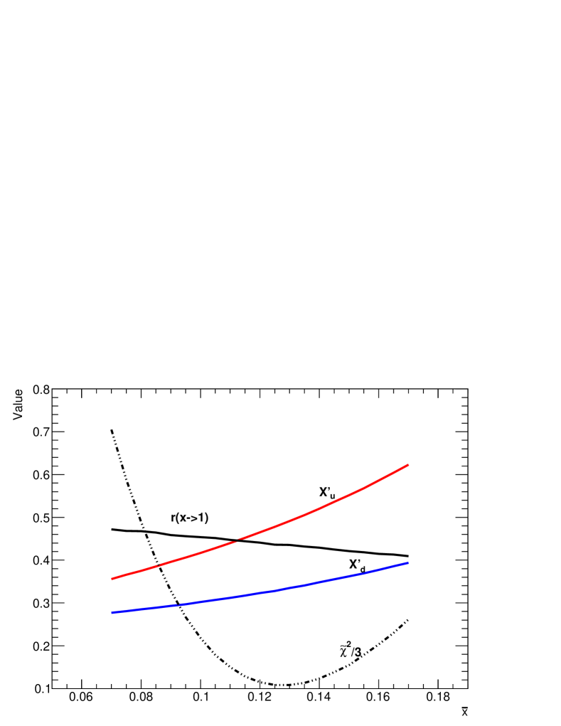
Figure 2: Normalized chi square ${\mathchoice{\raisebox{0.0pt}{$\displaystyle\tilde{\chi}$}}{\raisebox{0.0pt}{$\textstyle\tilde{\chi}$}}{\raisebox{0.0pt}{$\scriptstyle\tilde{\chi}$}}{\raisebox{0.0pt}{$\scriptscriptstyle\tilde{\chi}$}}}^{2}$ (dashed black), $X^{\prime}_{d}$ (blue), $X^{\prime}_{u}$ (red), and $r(x\rightarrow 1)$ (black) as a function of $\bar{x}$.

In Fig. 2, the mean ${\mathchoice{\raisebox{0.0pt}{$\displaystyle\tilde{\chi}$}}{\raisebox{0.0pt}{$\textstyle\tilde{\chi}$}}{\raisebox{0.0pt}{$\scriptstyle\tilde{\chi}$}}{\raisebox{0.0pt}{$\scriptscriptstyle\tilde{\chi}$}}}^{2}$ as a function of $\bar{x}$ is shown; it reaches its minimum at $\bar{x}=0.128$, which is somewhat larger than the previously determined value of $\bar{x}$ (see Eq. (12)) . Table 1 lists the values of $X^{\prime}_{u}$, $X^{\prime}_{d}$ and $r(x\rightarrow 1)$, respectively, obtained from the fit to the Marathon data using Eq. (19) and Eq. (23) for two different values of the parameter $\bar{x}$. The first $\bar{x}$ is from Eq. (12), while the second one corresponds to the location of minimal ${\mathchoice{\raisebox{0.0pt}{$\displaystyle\tilde{\chi}$}}{\raisebox{0.0pt}{$\textstyle\tilde{\chi}$}}{\raisebox{0.0pt}{$\scriptstyle\tilde{\chi}$}}{\raisebox{0.0pt}{$\scriptscriptstyle\tilde{\chi}$}}}^{2}$ in Fig. 2.

The comparison with the Marathon data for the two cases is shown in Fig. 1. Excellent agreement between the data and the calculation are found for the two cases, suggesting the relative insensitivity of $F^{n}_{2}(x)/F^{p}_{2}(x)$ to the exact values of the parameters adopted in the quantum statistical approach.

It is instructive to examine how the $F^{n}_{2}(x)/F^{p}_{2}(x)$ ratios vary for different ranges of $x$. The data from Marathon, as shown in Table 3 of Abrams2 , can be divided into two different $x$ ranges, [0.195, 0.51] and [0.51, 0.825]. One sees that the $F^{n}_{2}(x)/F^{p}_{2}(x)$ ratio decreases by $0.212\pm 0.026$ in the first range and only by $0.057\pm 0.019$ in the second, in good agreement with the quantum statistical approach.

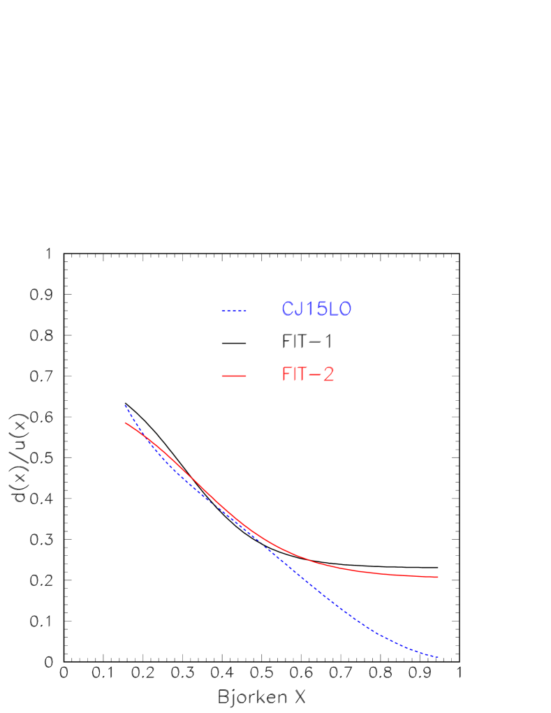
Figure 3: The $x$ dependence of $d(x)/u(x)$ for three proton PDFs. The dashed curve corresponds to the CJ15LO proton PDFs CJ . The solid curves correspond to the proton PDFs obtained from the statistical model using the two sets of parameters listed in Table I: $\bar{x}=0.099$ (black) and $\bar{x}=0.128$ (red), respectively.

Table 1: Evaluation of $X^{\prime}_{u}$, $X^{\prime}_{d}$ and $r(x)$ at $x\rightarrow 1$, respectively, from the fit to the Marathon data using Eq. (19) and Eq. (23) for two different values of the parameter $\bar{x}$. In the last column are the values of the normalized ${\mathchoice{\raisebox{0.0pt}{$\displaystyle\tilde{\chi}$}}{\raisebox{0.0pt}{$\textstyle\tilde{\chi}$}}{\raisebox{0.0pt}{$\scriptstyle\tilde{\chi}$}}{\raisebox{0.0pt}{$\scriptscriptstyle\tilde{\chi}$}}}^{2}$.

$\bar{x}$	$X^{\prime}_{u}$	$X^{\prime}_{d}$	$r(x\rightarrow 1)$	${\mathchoice{\raisebox{0.0pt}{$\displaystyle\tilde{\chi}$}}{\raisebox{0.0pt}{$\textstyle\tilde{\chi}$}}{\raisebox{0.0pt}{$\scriptstyle\tilde{\chi}$}}{\raisebox{0.0pt}{$\scriptscriptstyle\tilde{\chi}$}}}^{2}$
0.099	0.4148	0.3011	0.4394	0.68
0.128	0.4858	0.3321	0.4356	0.32

We also compare the $x$ dependence of $d(x)/u(x)$ with the proton PDFs obtained in the conventional parametrization and in the quantum statistical approach in Fig. 3. The dashed curve obtained with the CJ15LO proton PDFs CJ falls rapidly with $x$, approaching 0 as $x\to 1$. In contrast, the proton PDFs obtained from the quantum statistical approach, shown as the solid curves corresponding to the two sets of parameters in Table I, have a much slower fall off at large $x$. The distinct behavior of the $x$ dependence of $d(x)/u(x)$ is a result of the Fermi-Dirac form of the quark distribution in the quantum statistical approach.

In conclusion, we find that the large-$x$ behavior of the ratio $F^{n}_{2}(x)/F^{p}_{2}(x)$, measured with high precision by the Marathon experiment, favors the quantum statistical approach, which predicts that the ratio approaches a constant value greater than 1/4. The fact that the ratio decreases faster in the lower region of $x$ than in the higher region is also a property of the quantum statistical approach.

Unlike conventional parametrizations for the nucleon PDFs, the statistical approach has imposed specific forms for the parton distributions based on the Fermi-Dirac nature of the quarks and the Bose-Einstein nature of the gluons. Various predictions of the statistical approach are found to be in excellent agreement with existing data. Further stringent tests of the quantum statistical approach could be performed by considering the $Q^{2}$ dependence of the $F^{n}_{2}(x)/F^{p}_{2}(x)$ ratios, as well as the data for the polarized quark distributions.

It could be, finally, stressed that the distributions of the valence quarks at the large $x$ region show a big difference with the standard distributions. Our discussion of using quantum statistical mechanics for the proton PDFs could have implications for proton-proton collisions at the LHC.

References

-
(1)
1990 Nobel Lectures in Physics:
J. I. Friedman, Rev. Mod. Phys. 63, 615 (1991);
H. W. Kendall, Rev. Mod. Phys. 63, 597 (1991);
R. E. Taylor, Rev. Mod. Phys. 63, 573 (1991). - (2) J. I. Friedman and H. W. Kendall, Annu. Rev. Nucl. Sci. 22, 203 (1972).
- (3) J. J. Aubert et al., Nucl. Phys. B293, 740 (1987).
- (4) A. C. Benvenuti et al., Phys. Lett. B237, 599 (1990).
- (5) M. Arneodo et al., Nucl. Phys. B487, 3 (1997).
- (6) P. Berge et al., Z. Phys. C49, 187 (1991).
- (7) M. R. Adams et al., Phys. Rev. Lett. 75, 1466 (1995).
- (8) E. Oltman et al., Z. Phys. C53, 51 (1992).
- (9) F. E. Close, An Introduction to Quarks and Partons. Academic Press, London (1979).
- (10) O. Nachtmann, Nucl.Phys. B38, 397 (1972).
-
(11)
A. Bodek, M. Breidenbach, D. L. Dubin,
J. E. Elias, J. I. Friedman, H. W. Kendall, J. S. Poucher, E. M. Riordan,
M. R. Sogard, and D. H. Coward, Phys. Rev. Lett. 30, 1087 (1973).
J. S. Poucher et al., Phys. Rev. Lett. 32, 118 (1974). - (12) L. W. Whitlow, E. M. Riordan, S. Dasu, S. Rock, and A. Bodek, Phys. Lett. B282, 475 (1992).
- (13) W. Melnitchouk and A. W. Thomas, Phys. Lett. B377, 11 (1996).
- (14) I. R. Afnan et al., Phys. Lett. B493, 36 (2000).
-
(15)
D. Abrams et al., (Jefferson Laboratory, Hall A Tritium Collaboration),
Phys. Rev. Lett. 128, 132003 (2022).
arXiv 2104.05850[hep-ex]. - (16) A. Accardi, L. T. Brady, W. Melnitchouk, J. F. Owens, and N. Sato, Phys. Rev. D93, 114017 (2016).
- (17) H. Valenti, et al., arXiv:2210.04372[nucl-th].
-
(18)
T. J. Hague, J. Arrington, S. Li and S. N. Santiesteban,
Phys. Rev. C110, L041302 (2024).
arXiv:2312.13499[nucl-ex]. - (19) D. Abrams, et al., arXiv:2410.12099[nucl-ex].
-
(20)
S. Li, et al., Nature 609, 41 (2022).
arXiv:2210.04189[nucl-ex]. - (21) F. Gross, et al., arXiv:2212.11107[hep-ph].
-
(22)
J. Arrington, N. Formin and A. Schmidt,
Ann. Rev. Nucl. Part. Sci. 72, 307 (2022).
arXiv:2203.02608[nucl.ex]. -
(23)
P. Achenbach, et al., Nucl. Phys.
A1047, 122874 (2024).
arXiv:2303.02579[hep-ph]. -
(24)
J. Arrington, et al., Eur. Phy. J.
A59, 188 (2023).
arXiv:2304.09998[nucl-ex]. - (25) S. Alekhin, M. V. Garzelli, S. Kulagin and S.-O. Moch, arXiv:2306.01918[hep-ph].
-
(26)
Craig D. Roberts, Few-Body Syst. 64, art. n.51 (2023).
arXiv:2304.09998[nucl-ex]. - (27) A. Niegawa and K. Sasaki, Prog. Theor. Phys. 54, 192 (1975).
- (28) R. D. Field and R. P. Feynman, Phys. Rev. D15, 2590 (1977).
-
(29)
C. Bourrely, F. Buccella and J. Soffer,
Eur. Phys. J. C23, 487 (2002).
arXiv:hep-ph/0109160[hep-ph]. - (30) C. Bourrely, F. Buccella and J. Soffer, Mod. Phys. Lett. A18, 143 (2006) and Int. Jour. of Mod. Phys. 28, 13500 (2013).
-
(31)
V. N. Gribov and L. N. Lipatov, Sov. J. Nucl. Phys.
15, 478 (1972).
Yu. L. Dokshitzer, Sov. Phys. JETP 46, 641 (1977).
G. Altarelli and G. Parisi, Nucl. Phys. B126, 298 (1977). - (32) C. Bourrely and J. Soffer, Nucl. Phys. A941, 307 (2015).
- (33) C. Bourrely (to be published).
- (34) E. A. Hawker et al., Phys. Rev. Lett. 80, 3715 (1998).
- (35) J. C. Peng et al., Phys. Rev. D58, 092004 (1998).
- (36) R. S. Towell et al., Phys. Rev. D64, 052002 (2001).
- (37) J. Dove et al. (Sea-Quest Experiment), Nature 604, 7907 (2022).
- (38) J. Dove et al. (Sea-Quest Experiment), Phys. Rev. C108, 035202 (2023).
- (39) J. Adam et al., Phys. Rev. D99, 051102 (2019).
-
(40)
L. Bellantuono, R. Bellotti and F. Buccella, Mod. Phys. Lett. A38, 2350039 (2023).
arXiv:2201.076540[hep-ph]. -
(41)
M. Bonvini, F. Buccella, F. Giuli and F. Silvetti, Eur. Phys. J. 84, 541 (2024).
arXiv:2311.08785[hep-ph]. - (42) C. Bourrely, F. Buccella and J. C. Peng, Phys. Lett. B213 136021 (2021).
- (43) C. Bourrely, W. C. Cheng and J. C. Peng, Phys. Rev. D105, 076018 (2022).
-
(44)
C. Bourrely, F. Buccella, W. C. Cheng and J. C. Peng, Phys. Lett.
B828, 138395 (2024).
arXiv:2305.18117[hep-ph]. -
(45)
D. Abrams et al., (Jefferson Laboratory, Hall A Tritium
Collaboration), Supplement Online-Material-Tables of Measurements,
http://link.aps.org/supplemental/
10.1103/PhysRevLett.128.132003.