Bias in Gini coefficient estimation for gamma mixture populations

Abstract

This paper examines the properties of the Gini coefficient estimator for gamma mixture populations and reveals the presence of bias. In contrast, we show that sampling from a gamma distribution yields an unbiased estimator, consistent with prior research (Baydil et al.,, 2025). We derive an explicit bias expression for the Gini coefficient in gamma mixture populations, which serves as the foundation for proposing a bias-corrected Gini estimator. We conduct a Monte Carlo simulation study to evaluate the behavior of the bias-corrected Gini estimator.

Keywords. Gamma mixture distribution, Gini coefficient estimator, biased estimator.
Mathematics Subject Classification (2010). MSC 60E05 $\cdot$ MSC 62Exx $\cdot$ MSC 62Fxx.

1 Introduction

The Gini coefficient is a widely used measure of income inequality and dispersion in a population (Dorfman,, 1979). The degree of inequality within a distribution can be quantified using this method, which has applications in a variety of fields, including economics, finance, ecology, health, and environment, among others; see, for example, Damgaard and Weiner, (2000), Yao, (1999), Sun et al., (2010), and Kharazmi et al., (2023). According to Baydil et al., (2025), the Gini coefficient is commonly utilized by the World Bank in order to evaluate the degree of economic disparity that exists across countries. This highlights the practical significance of the Gini coefficient.

Mathematically, the Gini coefficient is commonly defined in terms of the expected absolute differences between two independent, identically distributed (i.i.d.) random variables. A widely used estimator for this index is the sample Gini coefficient; see Deltas, (2003). However, this estimator tends to be biased downward, particularly in small samples and across various distributions, including uniform, log-normal, and exponential models. To address this issue, Deltas, (2003) introduced the upward-adjusted sample Gini coefficient, which was shown to be unbiased when the population followed an exponential distribution. Recently, Baydil et al., (2025) extended the unbiasedness of the upward-adjusted sample Gini coefficient when the population follows a gamma distribution.

The gamma distribution is particularly appealing in economic modeling due to its flexibility in capturing mid-range income distributions, as opposed to the log-normal model, which is often used for high-income distributions; see Salem and Mount, (1974). McDonald and Jensen, (1979) derived the population Gini coefficient for a gamma-distributed population and explored its estimation via maximum likelihood and moment-based methods. Nevertheless, a single gamma distribution for modeling income may not be adequate as real-world income data is often heterogeneous, consisting of multiple economic classes (e.g., low-, middle-, and high-income earners). In contrast, a gamma mixture model can be a more flexible parametric model for an income distribution as studied by Chotikapanich and Griffiths, (2008). In fact, mixtures offer the benefit of a flexible functional structure while maintaining the convenience of parametric models that facilitate statistical inference; see Chotikapanich and Griffiths, (2008).

In this paper, we examine the estimation of the Gini coefficient in gamma mixture populations, a more general class of distributions that accounts for heterogeneity in income data. While the sample Gini coefficient is known to be an unbiased estimator for the population Gini coefficient in single gamma distributions (Baydil et al.,, 2025), we show that this property does not hold for gamma mixture models, leading to a systematic bias in estimation. Then, we derive an explicit expression for the bias and propose an unbiased Gini estimator when the population is gamma mixture distributed.

The rest of this paper unfolds as follows. In Section 2, we present the theoretical foundations and key definitions. In Section 3, we derive a closed-form expression for the expectation of the sample Gini coefficient estimator. In Section 4, we demonstrate the bias introduced when estimating the Gini coefficient from gamma mixture distributions, providing both theoretical and empirical evidence. In Section 5, we explore an Illustrative Monte Carlo simulation study. Finally, in Section 6, we provide some concluding remarks.

2 Preliminary results and some definitions

This section provides the theoretical foundation for our analysis, introducing preliminary results and definitions. A key result, Proposition 2.4, presents an explicit formula for the Gini coefficient, a widely used statistical measure of income inequality (Gini,, 1936).

The theoretical results presented in this section, pertaining to (almost surely) positive random variables, exhibit universal validity and applicability, transcending specific distributional forms and accommodating real-valued random variables with diverse support structures.

Lemma 2.1.

Let $X_{1}$ and $X_{2}$ be two independent copies of a (almost surely) positive random variable $X$ with finite integral and common cumulative distribution function $F$ and let $g$ be a positive real-valued integrable function of two (positive) variables. Then, the following identity holds:

$$\mathbb{E}[|X_{1}-X_{2}|g(X_{1},X_{2})]=2\mathbb{E}(X)\left\{\mathbb{E}\left[g(X^{*},X)\mathds{1}_{\{X<X^{*}\}}\right]-\mathbb{E}\left[g(X,X^{*})\mathds{1}_{\{X^{*}<X\}}\right]\right\},$$

where $\mathds{1}_{A}$ is the indicator function of an event $A$, $X^{*}$ is independent of $X$ and has length-biased distribution, that is, its cumulative distribution function is given by the following Lebesgue-Stieltjes integral:

$$F_{X^{*}}(u)={1\over\mathbb{E}(X)}\,{\int_{0}^{u}t{\rm d}F(t)},\quad u>0.$$ (1)

Proof.

From independence of $X_{1}$ and $X_{2}$, it follows that

$$\mathbb{E}[|X_{1}- X_{2}|g(X_{1},X_{2})]$$

$$=\int_{0}^{\infty}\left[\int_{u}^{\infty}(v-u)g(u,v){\rm d}F(v)\right]{\rm d}F(u)+\int_{0}^{\infty}\left[\int_{0}^{u}(u-v)g(u,v){\rm d}F(v)\right]{\rm d}F(u)$$

$$=2\int_{0}^{\infty}u\left[\int_{0}^{u}g(u,v){\rm d}F(v)\right]{\rm d}F(u)-2\int_{0}^{\infty}\left[\int_{0}^{u}vg(u,v){\rm d}F(v)\right]{\rm d}F(u),$$ (2)

where in the last identity we use the fact that $X_{1}$ and $X_{2}$ are identically distributed. By using the definition (1) of $F_{X^{*}}$, the expression in (2) can be written as

$$2\mathbb{E}(X)\int_{0}^{\infty}\left[\int_{0}^{u}g(u,v){\rm d}F(v)\right]{\rm d}F_{X^{*}}(u)-2\mathbb{E}(X)\int_{0}^{\infty}\left[\int_{0}^{u}g(u,v){\rm d}F_{X^{*}}(v)\right]{\rm d}F(u).$$

Hence the proof readily follows. ∎

Proposition 2.2.

Under the conditions of Lemma 2.1, if $g$ is symmetric, that is, $g(u,v)=g(v,u)$, $u,v>0$, then

$$\mathbb{E}[|X_{1}-X_{2}|g(X_{1},X_{2})]=2\mathbb{E}(X)\left\{2\mathbb{E}\left[g(X^{*},X)\mathds{1}_{\{X<X^{*}\}}\right]-\mathbb{E}\left[g(X^{*},X)\right]+\mathbb{E}\left[g(X^{*},X)\mathds{1}_{\{X=X^{*}\}}\right]\right\}.$$

Proof.

The proof is immediate, therefore omitted. ∎

Proposition 2.3.

Under the conditions of Proposition 2.2, we have

$$\mathbb{E}(|X_{1}-X_{2}|)=2\mathbb{E}(X)\left[2\mathbb{P}(X<X^{*})-1+\mathbb{P}(X=X^{*})\right].$$ (3)

Equivalently,

$$\mathbb{E}(|X_{1}-X_{2}|)=2\mathbb{E}(X)\left[2F_{X\over X+X^{*}}\left({1\over 2}\right)-1+\mathbb{P}(X=X^{*})\right],$$ (4)

with $F_{X/(X+X^{*})}$ being the cumulative distribution function of the independent ratio ${X/(X+X^{*})}$.

Proof.

By taking, in Lemma 2.1, $g$ as the unitary constant function, we obtain (3). Identity in (4) follows from the equality of events $\{X<X^{*}\}$ and $\{2X<X+X^{*}\}$. ∎

The Gini coefficient is defined using the Lorenz curve, which plots cumulative income share against population percentage. The line of perfect equality is a 45-degree line. The Gini coefficient is calculated as the ratio of the area between the Lorenz curve and the line of equality to the total area under the line. To derive explicit expressions, we use the standard definition based on the mean difference.

Definition 2.1.

The Gini coefficient (Gini,, 1936) of a random variable $X$ with finite mean $\mathbb{E}(X)$ is defined as

$$G={1\over 2}\,{\mathbb{E}(|X_{1}-X_{2}|)\over\mathbb{E}(X)},$$ (5)

where $X_{1}$ and $X_{2}$ are independent copies of $X$.

Proposition 2.4.

Under the conditions of Proposition 2.3, the Gini coefficient for $X$ is given by

$$G=2F_{X\over X+X^{*}}\left({1\over 2}\right)-1+\mathbb{P}(X=X^{*}),$$

with $F_{X/(X+X^{*})}$ being the cumulative distribution function of the independent ratio ${X/(X+X^{*})}$ and $X^{*}$ distributed according to (1).

We proceed by defining the gamma mixture distribution for the case of a constant rate parameter, $\lambda>0$. While our results can be extended to the more general case of non-constant rate parameters, our primary goal is to investigate the bias in the estimation of the Gini coefficient for a gamma mixture distribution, and we demonstrate that this can be achieved by focusing on the constant $\lambda$ scenario.

Definition 2.2.

A random variable $X$ has a gamma mixture distribution (Kitani et al.,, 2024) with parameter vector $\bm{\theta}=(\pi_{1},\ldots,\pi_{m},\alpha_{1},\ldots,\alpha_{m},\lambda)^{\top}$, denoted by $X\sim\text{GM}(\bm{\theta})$, if it has the following mixture density:

$$f(x;\bm{\theta})=\sum_{i=1}^{m}\pi_{i}g_{i}(x;\alpha_{i},\lambda),\quad x>0,$$

where $m\in\mathbb{N}$ denotes the number of components, $\pi_{i}$ denotes the mixing proportion such that $\sum_{i=1}^{m}\pi_{i}=1$, $\pi_{i}>0$, and $g_{i}$ is the density of the gamma distribution with shape parameter $\alpha_{i}>0$ and rate parameter $\lambda>0$, that is,

$$g_{i}(x;\alpha_{i},\lambda)={\lambda^{\alpha_{i}}\over\Gamma(\alpha_{i})}\,x^{\alpha_{i}-1}\exp(-\lambda x),\quad x>0,$$ (6)

where $\Gamma(\cdot)$ denotes the (complete) gamma function.

The gamma mixture distribution is a comprehensive framework that encompasses a broad range of important distributions, as illustrated in Figure 1 (adaptation of Figure 1 of Kitani et al.,, 2024).

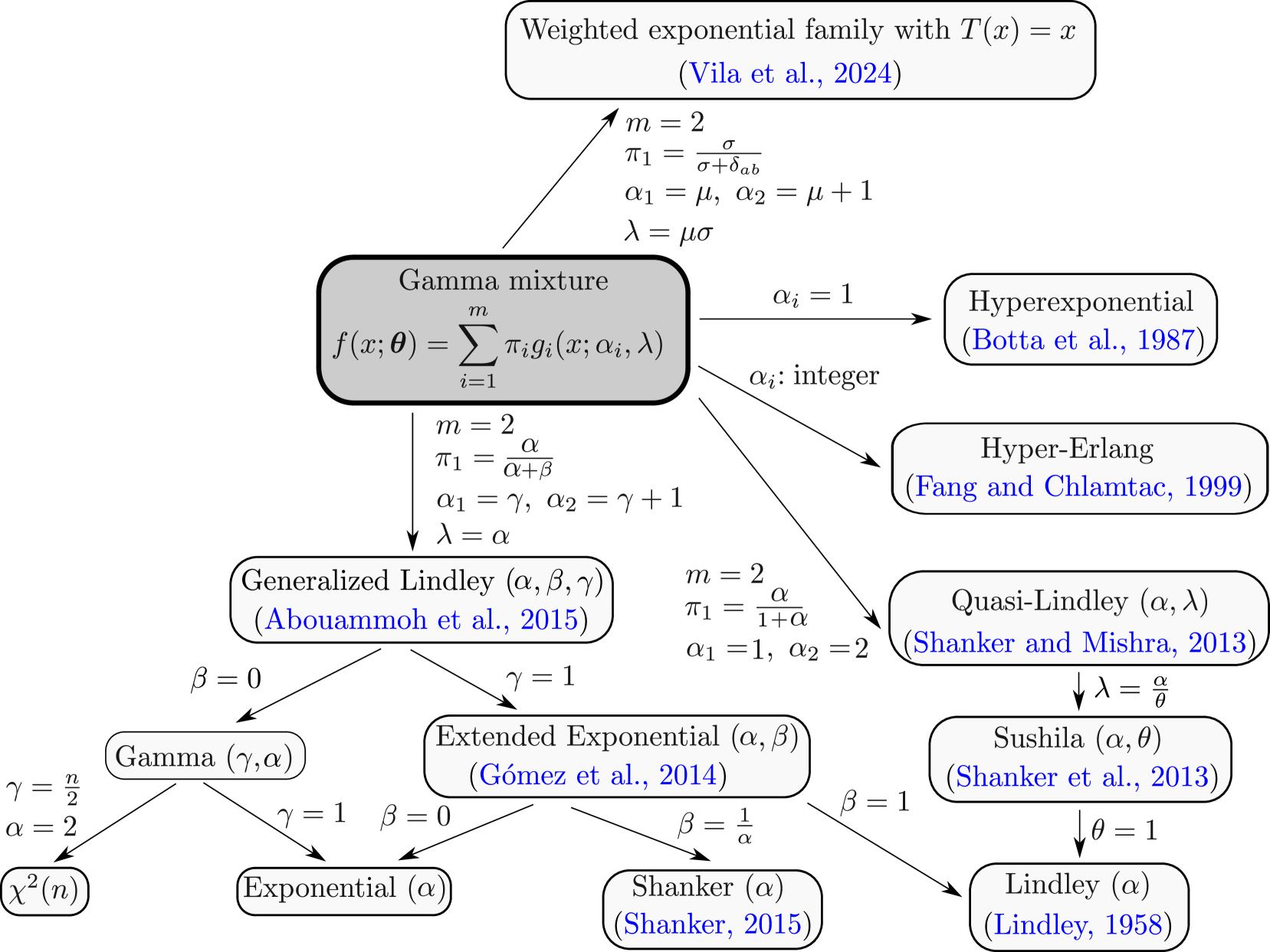
Figure 1: Gamma mixture-type distribution relationships.

Example 2.1.

If $X\sim\text{GM}(\bm{\theta})$, then $X^{*}\sim\text{GM}(\bm{\theta}^{*})$, where $\bm{\theta}^{*}=(\pi^{*}_{1},\ldots,\pi^{*}_{m},\alpha_{1}+1,\ldots,\alpha_{m}+1,\lambda)^{\top}$, and

$$\pi^{*}_{j}\equiv{\pi_{j}\alpha_{j}\over\sum_{k=1}^{m}{\pi_{k}\alpha_{k}}},\quad j=1,\ldots,m.$$ (7)

As $X$ and $X^{*}$ are independent, by Jacobian method the density of the ratio ${X/(X+X^{*})}$ satisfies:

$$f_{{X\over X+X^{*}}}(z) =(s+1)^{2}\int_{0}^{\infty}xf(x;\bm{\theta})f(sx;\bm{\theta}^{*}){\rm d}x,\quad s={1\over z}-1,\ 0<z<1.$$ (8)

By using the definitions of $f(x;\bm{\theta})$ and $f(sx;\bm{\theta}^{*})$ in (8),

$$f_{{X\over X+X^{*}}}(z) =(s+1)^{2}\sum_{i,j=1}^{m}\pi_{i}\pi_{j}^{*}{\lambda^{\alpha_{i}+\alpha_{j}+1}\over\Gamma(\alpha_{i})\Gamma(\alpha_{j}+1)}\,s^{\alpha_{j}}\int_{0}^{\infty}x^{\alpha_{i}+\alpha_{j}}\exp[-\lambda(1+s)x]{\rm d}x$$

$$=\sum_{i,j=1}^{m}\pi_{i}\pi_{j}^{*}\,{z^{\alpha_{i}-1}(1-z)^{\alpha_{j}}\over\text{B}(\alpha_{i},\alpha_{j}+1)},\quad 0<z<1,$$

where $\text{B}(\cdot,\cdot)$ is the (complete) beta function. That is, the distribution of ${X/(X+X^{*})}$ is a mixture of beta distributions with parameters $\alpha_{i}$ and $\alpha_{j}+1$, $i,j=1,\ldots,m$. Then, the cumulative distribution function of ${X/(X+X^{*})}$ can be written as

$$F_{{X\over X+X^{*}}}(z)=\sum_{i,j=1}^{m}\pi_{i}\pi_{j}^{*}\,{\text{B}(z;\alpha_{i},\alpha_{j}+1)\over\text{B}(\alpha_{i},\alpha_{j}+1)}=\sum_{i,j=1}^{m}\pi_{i}\pi_{j}^{*}\,{{}_{2}F_{1}\left(\alpha_{i},-\alpha_{j};\alpha_{i}+1;z\right)\over\alpha_{i}\text{B}(\alpha_{i},\alpha_{j}+1)}\,z^{\alpha_{i}},\quad 0<z<1,$$

where we have used the well-known identity $\text{B}(x;a,b)=(x^{a}/a)\,_{2}F_{1}(a,1-b;a+1;x)$ that relates the incomplete beta function $\text{B}(x;a,b)$ to the hypergeometric function ${}_{2}F_{1}(a,b;c;x)$. Applying Proposition 2.4, the Gini coefficient of the GM distribution can be expressed as

$$G=\sum_{i,j=1}^{m}\pi_{i}\pi_{j}^{*}\,{{}_{2}F_{1}\left(\alpha_{i},-\alpha_{j};\alpha_{i}+1;{1\over 2}\right)\over 2^{\alpha_{i}-1}\alpha_{i}\text{B}(\alpha_{i},\alpha_{j}+1)}-1,$$ (9)

because $\mathbb{P}(X=X^{*})=0$.

Example 2.2.

By taking $m=1$, $\pi_{1}=\pi_{1}^{*}=1$ and $\alpha_{1}=\alpha_{2}=\alpha$ in (9), we have

$$G={{}_{2}F_{1}\left(\alpha,-\alpha;\alpha+1;{1\over 2}\right)\over 2^{\alpha-1}\alpha B(\alpha,\alpha+1)}-1.$$ (10)

By using the identity (Wolfram Research,, 2024):

$$\,{}_{2}F_{1}\left(a,-a;c;{1\over 2}\right)={\sqrt{\pi}\Gamma(c)\over 2^{c}}\left[{1\over\Gamma({a+c+1\over 2})\Gamma({c-a\over 2})}+{1\over\Gamma({a+c\over 2})\Gamma({c-a+1\over 2})}\right],$$

the Gini coefficient (10) becomes

$$G={\Gamma(2\alpha+1)\over\alpha^{2}2^{2\alpha}\Gamma^{2}(\alpha)}+{2^{1-2\alpha}\sqrt{\pi}\Gamma(2\alpha)\over\Gamma(\alpha)\Gamma(\alpha+{1\over 2})}-1={\Gamma(2\alpha+1)\over\alpha^{2}2^{2\alpha}\Gamma^{2}(\alpha)},$$ (11)

where in the last equality we have used the Legendre duplication formula (Abramowitz and Stegun,, 1972): $\Gamma(x)\Gamma\left(x+{1/2}\right)=2^{1-2x}\sqrt{\pi}\Gamma(2x).$ Again, by applying Legendre duplication formula in (11), we get the following expression

$$G={\Gamma(\alpha+{1\over 2})\over\sqrt{\pi}\alpha\Gamma(\alpha)},$$

which is consistent with the well-known formula for the Gini coefficient of the gamma distribution, as reported in the existing literature (see, for example, McDonald and Jensen,, 1979).

3 The main result

Utilizing the foundational results presented in Section 2, is this part, we obtain a simple closed-form expression (Theorem 3.1) for the expected value of the Gini coefficient estimator $\widehat{G}$, initially proposed by Deltas, (2003),

$$\widehat{G}={1\over n-1}\left[\dfrac{\displaystyle\sum_{1\leqslant i<j\leqslant n}|X_{i}-X_{j}|}{\displaystyle\sum_{i=1}^{n}X_{i}}\right],\quad n\in\mathbb{N},\,n\geqslant 2,$$ (12)

where $X_{1},X_{2},\ldots,X_{n}$ are i.i.d. observations from the population.

The following theorem is valid only for (almost surely) positive random variables and its proof adapts similar technical steps as reference Baydil et al., (2025).

Theorem 3.1.

Let $X_{1},X_{2},\ldots$ be independent copies of a (almost surely) positive random variable $X$ with finite integral and common cumulative distribution function $F$. The following holds:

$$\mathbb{E}(\widehat{G})=n\mathbb{E}(X)\left\{2R_{1}(F)-R_{\infty}(F)+\mathbb{E}\left[g(X^{*},X)\mathds{1}_{\{X=X^{*}\}}\right]\right\},\quad n\in\mathbb{N},\,n\geqslant 2,$$

where $X^{*}$ has length-biased distribution (see Lemma 2.1), $R_{1}(F)\equiv\lim_{\varepsilon\to 1}R_{\varepsilon}(F)$, $R_{\infty}(F)\equiv\lim_{\varepsilon\to\infty}R_{\varepsilon}(F)$,

$$R_{\varepsilon}(F)\equiv\int_{0}^{\infty}\mathbb{E}\left[\exp\left(-xX^{*}\right)H(x,\varepsilon X^{*})\right]\mathscr{L}^{n-2}_{F}(x){\rm d}x,\quad\varepsilon>0,$$ (13)

$$H(x,x^{*})\equiv\int_{0}^{x^{*}}\exp\left(-xu\right){\rm d}F(u),\quad x,x^{*}>0,$$ (14)

$${g}(u,v)\equiv\int_{0}^{\infty}\exp\left\{-(u+v)x\right\}\mathscr{L}^{n-2}_{F}(x){\rm d}x,\quad u,v>0,$$ (15)

and $\mathscr{L}_{F}(p)=\int_{0}^{\infty}\exp(-pu){\rm d}F(u)$ is the Laplace transform corresponding to distribution $F$. In the above, we are assuming that the Lebesgue-Stieltjes integrals and improper integrals involved exist.

Proof.

By using the very well-known identity

$${z}\int_{0}^{\infty}\exp(-zx){\rm d}x=1,$$

with $z=\sum_{i=1}^{n}X_{i}$, and by taking advantage of the independent and identically distributive nature of $X_{1},X_{2},\ldots$, we have

$$\mathbb{E}\left[\dfrac{\displaystyle\sum_{1\leqslant i<j\leqslant n}|X_{i}-X_{j}|}{\displaystyle\sum_{i=1}^{n}X_{i}}\right] =\mathbb{E}\left[\sum_{1\leqslant i<j\leqslant n}|X_{i}-X_{j}|\int_{0}^{\infty}\exp\left\{-\left(\displaystyle\sum_{i=1}^{n}X_{i}\right)x\right\}{\rm d}x\right]$$

$$=\mathbb{E}\left[\sum_{1\leqslant i<j\leqslant n}|X_{i}-X_{j}|\int_{0}^{\infty}\exp\left\{-(X_{1}+X_{2})x\right\}\exp\left\{-\left(\displaystyle\sum_{i=3}^{n}X_{i}\right)x\right\}{\rm d}x\right]$$

$$=\binom{n}{2}\mathbb{E}\left[|X_{1}-X_{2}|\int_{0}^{\infty}\exp\left\{-(X_{1}+X_{2})x\right\}\mathscr{L}^{n-2}_{F}(x){\rm d}x\right].$$ (16)

By taking ${g}(u,v)$ as in (15), the identity in (16) can be written as

$$\mathbb{E}\left[\dfrac{\displaystyle\sum_{1\leqslant i<j\leqslant n}|X_{i}-X_{j}|}{\displaystyle\sum_{i=1}^{n}X_{i}}\right]=\binom{n}{2}\mathbb{E}\left[|X_{1}-X_{2}|{g}(X_{1},X_{2})\right].$$

As ${g}$ in (15) is symmetric, by applying Proposition 2.2, the above identity becomes

$$\mathbb{E}(\widehat{G})=n\mathbb{E}(X)\left\{2\mathbb{E}\left[g(X^{*},X)\mathds{1}_{\{X<X^{*}\}}\right]-\mathbb{E}\left[g(X^{*},X)\right]+\mathbb{E}\left[g(X^{*},X)\mathds{1}_{\{X=X^{*}\}}\right]\right\}.$$ (17)

Now, note that

$$\mathbb{E}\left[{g}(X^{*},X)\mathds{1}_{\{X<X^{*}\}}\right] =\int_{0}^{\infty}\mathbb{E}\left[\exp\left\{-(X^{*}+X)x\right\}\mathds{1}_{\{X<X^{*}\}}\right]\mathscr{L}^{n-2}_{F}(x){\rm d}x$$

$$=\int_{0}^{\infty}\mathbb{E}\left[\exp\left(-xX^{*}\right)\int_{0}^{\infty}\exp\left(-xu\right)\mathds{1}_{\{u<X^{*}\}}{\rm d}F(u)\right]\mathscr{L}^{n-2}_{F}(x){\rm d}x$$ (18)

and

$$\mathbb{E}\left[{g}(X^{*},X)\right] =\int_{0}^{\infty}\mathbb{E}\left[\exp\left\{-(X^{*}+X)x\right\}\right]\mathscr{L}^{n-2}_{F}(x){\rm d}x$$

$$=\int_{0}^{\infty}\mathbb{E}\left[\exp\left(-xX^{*}\right)\int_{0}^{\infty}\exp\left(-xu\right){\rm d}F(u)\right]\mathscr{L}^{n-2}_{F}(x){\rm d}x.$$ (19)

By replacing (3) and (3) in formula (17), and by using the notations in (13) and (14), the proof of the theorem readily follows. ∎

Remark 3.2.

Note that the Laplace transform corresponding to distribution $F$ can be obtained from $H(\cdot,\cdot)$ in (14) as follows:

$$\mathscr{L}_{F}(x)=\lim_{\varepsilon\to\infty}H(x,\varepsilon x^{*}),\quad x,x^{*}>0.$$

As an immediate consequence of Theorem 3.1, the following result follows.

Corollary 3.3.

Under the conditions of Theorem 3.1, with $X$ being a (almost surely) positive, absolutely continuous random variable with finite integral and common cumulative distribution function $F$, we have

$$\mathbb{E}(\widehat{G})=n\mathbb{E}(X)\left[2R_{1}(F)-R_{\infty}(F)\right],\quad n\in\mathbb{N},\,n\geqslant 2.$$

4 The Gini coefficient estimator is biased for gamma mixtures

In this section, we show that the estimator $\widehat{G}$ in (12) of the Gini coefficient $G$ (given in Example 2.1) for a gamma mixture population is biased, whereas sampling from a gamma-distributed population eliminates this bias, as previously established by Baydil et al., (2025).

Indeed, if $X\sim\text{GM}(\bm{\theta})$ (see Definition 2.2), then, $H(\cdot,\cdot)$ in (14) can be written as

$$H(x,\varepsilon x^{*}) =\sum_{i=1}^{m}\pi_{i}\int_{0}^{\varepsilon x^{*}}\exp\left(-xu\right)g_{i}(u;\alpha_{i},\lambda){\rm d}u,\quad x,x^{*},\varepsilon>0,$$

$$=\sum_{i=1}^{m}\pi_{i}\,{\lambda^{\alpha_{i}}\over\Gamma(\alpha_{i})}\int_{0}^{\varepsilon x^{*}}u^{\alpha_{i}-1}\exp[-(x+\lambda)u]{\rm d}u$$

$$=\sum_{i=1}^{m}\pi_{i}\,\left({\lambda\over x+\lambda}\right)^{\alpha_{i}}{\gamma(\alpha_{i},(x+\lambda)\varepsilon x^{*})\over\Gamma(\alpha_{i})},$$ (20)

with $g_{i}(\cdot;\alpha_{i},\lambda)$ being as in (15). By using Remark 3.2, from (4), we obtain

$$\mathscr{L}_{F}(x)=\lim_{\varepsilon\to\infty}H(x,\varepsilon x^{*})=\sum_{i=1}^{m}\pi_{i}\,\left({\lambda\over x+\lambda}\right)^{\alpha_{i}},\quad x,x^{*}>0,$$ (21)

where the well-known identity $\Gamma(x)=\lim_{y\to\infty}\gamma(x,y)$ has been used. Furthermore, since $X^{*}\sim\text{GM}(\bm{\theta}^{*})$ with $\bm{\theta}^{*}$ being as in Example 2.1, by using (4), we have

$$\mathbb{E}[\exp\left(-xX^{*}\right) H(x,\varepsilon X^{*})]=\sum_{i=1}^{m}\pi_{i}\,\left({\lambda\over x+\lambda}\right)^{\alpha_{i}}{1\over\Gamma(\alpha_{i})}\,\mathbb{E}\left[\exp\left(-xX^{*}\right)\gamma(\alpha_{i},(x+\lambda)\varepsilon X^{*})\right]$$

$$=\sum_{i,j=1}^{m}\pi_{i}\pi_{j}^{*}\,\left({\lambda\over x+\lambda}\right)^{\alpha_{i}}{\lambda^{\alpha_{j}+1}\over\Gamma(\alpha_{i})\Gamma(\alpha_{j}+1)}\int_{0}^{\infty}v^{\alpha_{j}}\exp\left[-(x+\lambda)v\right]\gamma(\alpha_{i},(x+\lambda)\varepsilon v){\rm d}v$$

$$=\sum_{i,j=1}^{m}\pi_{i}\pi_{j}^{*}\,{\lambda^{\alpha_{j}+1}\over\alpha_{i}B(\alpha_{i},\alpha_{j}+1)}\left({\lambda\over x+\lambda}\right)^{\alpha_{i}}{(x+\lambda)^{\alpha_{i}}\varepsilon^{\alpha_{i}}\over[(x+\lambda)\varepsilon+x+\lambda]^{\alpha_{i}+\alpha_{j}+1}}$$

$$\times\,_{2}F_{1}\left(\alpha_{i}+\alpha_{j}+1,1;\alpha_{i}+1;{\varepsilon\over\varepsilon+1}\right),$$

where in the last line the identity (D’Aurizio,, 2016):

$$\int_{0}^{\infty}x^{a-1}\exp(-sx)\gamma(b,\theta x){\rm d}x={\theta^{b}\Gamma(a+b)\over b(s+\theta)^{a+b}}\,_{2}F_{1}\left(a+b,1;b+1;{\theta\over s+\theta}\right),$$

has been used.

Hence, $R_{\varepsilon}(F)$ in (13) can be written as

$$R_{\varepsilon}(F) =\int_{0}^{\infty}\mathbb{E}\left[\exp\left(-xX^{*}\right)H(x,\varepsilon X^{*})\right]\mathscr{L}^{n-2}_{F}(x){\rm d}x$$

$$=\sum_{i,j=1}^{m}\pi_{i}\pi_{j}^{*}\,{\lambda^{\alpha_{j}+1}\over\alpha_{i}B(\alpha_{i},\alpha_{j}+1)}\,_{2}F_{1}\left(\alpha_{i}+\alpha_{j}+1,1;\alpha_{i}+1;{\varepsilon\over\varepsilon+1}\right)$$

$$\times\int_{0}^{\infty}{{\lambda}^{\alpha_{i}}\varepsilon^{\alpha_{i}}\over[(x+\lambda)\varepsilon+x+\lambda]^{\alpha_{i}+\alpha_{j}+1}}\mathscr{L}^{n-2}_{F}(x){\rm d}x.$$ (22)

Furthermore, by using, in (4), the Euler’s Hypergeometric transformation (Abramowitz and Stegun,, 1972): ${}_{2}F_{1}(a,b;c;x)=(1-x)^{c-a-b}{}_{2}F_{1}(c-a,c-b;c;x)$, we have

$$R_{\varepsilon}(F)=\sum_{i,j=1}^{m}\pi_{i}\pi_{j}^{*}\,{\,{}_{2}F_{1}\left(-\alpha_{j},\alpha_{i};\alpha_{i}+1;{\varepsilon\over\varepsilon+1}\right)\over\alpha_{i}B(\alpha_{i},\alpha_{j}+1)}\left({\varepsilon\over\varepsilon+1}\right)^{\alpha_{i}}\int_{0}^{\infty}\left({\lambda\over x+\lambda}\right)^{\alpha_{i}+\alpha_{j}+1}\mathscr{L}^{n-2}_{F}(x){\rm d}x.$$ (23)

Now, by taking $\varepsilon\to 1$ in (23), from formula (21) of $\mathscr{L}_{F}(x)$, we get

$$R_{1}(F)=\sum_{i,j=1}^{m}\pi_{i}\pi_{j}^{*}\,{{}_{2}F_{1}\left(-\alpha_{j},\alpha_{i};\alpha_{i}+1;{1\over 2}\right)\over 2^{\alpha_{i}}\alpha_{i}B(\alpha_{i},\alpha_{j}+1)}\int_{0}^{\infty}\left({\lambda\over x+\lambda}\right)^{\alpha_{i}+\alpha_{j}+1}\mathscr{L}^{n-2}_{F}(x){\rm d}x$$

$$=\sum_{i,j=1}^{m}\pi_{i}\pi_{j}^{*}\,{{}_{2}F_{1}\left(-\alpha_{j},\alpha_{i};\alpha_{i}+1;{1\over 2}\right)\over 2^{\alpha_{i}}\alpha_{i}B(\alpha_{i},\alpha_{j}+1)}\sum_{1\leqslant i_{1},\ldots,i_{n-2}\leqslant m}\pi_{i_{1}}\cdots\pi_{i_{n-2}}\int_{0}^{\infty}\left({\lambda\over x+\lambda}\right)^{\alpha_{i_{1}}+\cdots+\alpha_{i_{n-2}}+\alpha_{i}+\alpha_{j}+1}{\rm d}x$$

$$=\lambda\sum_{i,j=1}^{m}\pi_{i}\pi_{j}^{*}\,{{}_{2}F_{1}\left(-\alpha_{j},\alpha_{i};\alpha_{i}+1;{1\over 2}\right)\over 2^{\alpha_{i}}\alpha_{i}B(\alpha_{i},\alpha_{j}+1)}\sum_{1\leqslant i_{1},\ldots,i_{n-2}\leqslant m}\pi_{i_{1}}\cdots\pi_{i_{n-2}}\,{1\over\alpha_{i_{1}}+\cdots+\alpha_{i_{n-2}}+\alpha_{i}+\alpha_{j}}.$$ (24)

On the other hand, by setting $\varepsilon\to\infty$ in (23), from formula (21) of $\mathscr{L}_{F}(x)$ and from definition (7) of $\pi_{j}^{*}$, we obtain

$$R_{\infty}(F) =\sum_{i,j=1}^{m}\pi_{i}\pi_{j}^{*}\,{\,{}_{2}F_{1}\left(-\alpha_{j},\alpha_{i};\alpha_{i}+1;1\right)\over\alpha_{i}B(\alpha_{i},\alpha_{j}+1)}\int_{0}^{\infty}\left({\lambda\over x+\lambda}\right)^{\alpha_{i}+\alpha_{j}+1}\mathscr{L}^{n-2}_{F}(x){\rm d}x$$

$$={1\over\sum_{k=1}^{m}{\pi_{k}\alpha_{k}}}\sum_{j=1}^{m}\pi_{j}\alpha_{j}\int_{0}^{\infty}\left({\lambda\over x+\lambda}\right)^{\alpha_{j}+1}\mathscr{L}^{n-1}_{F}(x){\rm d}x$$

$$={1\over\sum_{k=1}^{m}{\pi_{k}\alpha_{k}}}\sum_{j=1}^{m}\pi_{j}\alpha_{j}\sum_{1\leqslant i_{1},\ldots,i_{n-1}\leqslant m}\pi_{i_{1}}\cdots\pi_{i_{n-1}}\int_{0}^{\infty}\left({\lambda\over x+\lambda}\right)^{\alpha_{i_{1}}+\cdots+\alpha_{i_{n-1}}+\alpha_{j}+1}{\rm d}x$$

$$={1\over\sum_{k=1}^{m}{\pi_{k}\alpha_{k}\over\lambda}}\sum_{1\leqslant i_{1},\ldots,i_{n-1}\leqslant m}\pi_{i_{1}}\cdots\pi_{i_{n-1}}\,\sum_{j=1}^{m}{\pi_{j}\alpha_{j}\over\alpha_{i_{1}}+\cdots+\alpha_{i_{n-1}}+\alpha_{j}},$$ (25)

where in the second equality the identity $\,{}_{2}F_{1}\left(-\alpha_{j},\alpha_{i};\alpha_{i}+1;1\right)=\alpha_{i}B(\alpha_{i},\alpha_{j}+1)$ has been used.

Then, by using (4) and (4), from Corollary 3.3, we get

$$\mathbb{E}(\widehat{G}) =n\mathbb{E}(X)\left[2R_{1}(F)-R_{\infty}(F)\right]$$

$$=\sum_{i,j=1}^{m}\pi_{i}\pi_{j}^{*}\,{{}_{2}F_{1}\left(-\alpha_{j},\alpha_{i};\alpha_{i}+1;{1\over 2}\right)\over 2^{\alpha_{i}-1}\alpha_{i}B(\alpha_{i},\alpha_{j}+1)}\left[\sum_{1\leqslant i_{1},\ldots,i_{n-2}\leqslant m}\pi_{i_{1}}\cdots\pi_{i_{n-2}}\,{n\sum_{k=1}^{m}{\pi_{k}\alpha_{k}}\over\alpha_{i_{1}}+\cdots+\alpha_{i_{n-2}}+\alpha_{i}+\alpha_{j}}\right]$$

$$-\sum_{1\leqslant i_{1},\ldots,i_{n-1}\leqslant m}\pi_{i_{1}}\cdots\pi_{i_{n-1}}\,\sum_{j=1}^{m}{n\pi_{j}\alpha_{j}\over\alpha_{i_{1}}+\cdots+\alpha_{i_{n-1}}+\alpha_{j}},$$ (26)

because $\mathbb{P}(X=X^{*})=0$.

Therefore, by (26) and (9), the bias of $\widehat{G}$ relative to $G$, denoted by $\text{Bias}(\widehat{G},G)$, can be written as

$$\text{Bias}(\widehat{G},G) =\sum_{i,j=1}^{m}\pi_{i}\pi_{j}^{*}\,{{}_{2}F_{1}\left(-\alpha_{j},\alpha_{i};\alpha_{i}+1;{1\over 2}\right)\over 2^{\alpha_{i}-1}\alpha_{i}B(\alpha_{i},\alpha_{j}+1)}\left[\sum_{1\leqslant i_{1},\ldots,i_{n-2}\leqslant m}\pi_{i_{1}}\cdots\pi_{i_{n-2}}\,{n\sum_{k=1}^{m}{\pi_{k}\alpha_{k}}\over\alpha_{i_{1}}+\cdots+\alpha_{i_{n-2}}+\alpha_{i}+\alpha_{j}}-1\right]$$

$$+\left[1-\sum_{1\leqslant i_{1},\ldots,i_{n-1}\leqslant m}\pi_{i_{1}}\cdots\pi_{i_{n-1}}\,\sum_{j=1}^{m}{n\pi_{j}\alpha_{j}\over\alpha_{i_{1}}+\cdots+\alpha_{i_{n-1}}+\alpha_{j}}\right].$$ (27)

Remark 4.1.

Note that $\text{Bias}(\widehat{G},G)=0$ if and only $\alpha_{1}=\cdots=\alpha_{m}=\alpha$, that is, the estimator $\widehat{G}$ is unbiased when sampling from a gamma distribution (Baydil et al.,, 2025).

5 Illustrative simulation study

Note that a bias-corrected Gini estimator can then be proposed from (9) and (4) as

$$\widehat{G}_{\text{bc}} =\widehat{G}-\text{Bias}(\widehat{G},G)$$

$$=\left[\sum_{i,j=1}^{m}\widehat{\pi}_{i}\widehat{\pi}_{j}^{*}\,{{}_{2}F_{1}\left(\widehat{\alpha}_{i},-\widehat{\alpha}_{j};\widehat{\alpha}_{i}+1;{1\over 2}\right)\over 2^{\widehat{\alpha}_{i}-1}\widehat{\alpha}_{i}B(\widehat{\alpha}_{i},\widehat{\alpha}_{j}+1)}-1\right]$$

$$-\sum_{i,j=1}^{m}\widehat{\pi}_{i}\widehat{\pi}_{j}^{*}\,{{}_{2}F_{1}\left(-\widehat{\alpha}_{j},\widehat{\alpha}_{i};\widehat{\alpha}_{i}+1;{1\over 2}\right)\over 2^{\widehat{\alpha}_{i}-1}\widehat{\alpha}_{i}B(\widehat{\alpha}_{i},\widehat{\alpha}_{j}+1)}\left[\sum_{1\leqslant i_{1},\ldots,i_{n-2}\leqslant m}\widehat{\pi}_{i_{1}}\cdots\widehat{\pi}_{i_{n-2}}\,{n\sum_{k=1}^{m}{\widehat{\pi}_{k}\widehat{\alpha}_{k}}\over\widehat{\alpha}_{i_{1}}+\cdots+\widehat{\alpha}_{i_{n-2}}+\widehat{\alpha}_{i}+\widehat{\alpha}_{j}}-1\right]$$

$$-\left[1-\sum_{1\leqslant i_{1},\ldots,i_{n-1}\leqslant m}\widehat{\pi}_{i_{1}}\cdots\widehat{\pi}_{i_{n-1}}\,\sum_{j=1}^{m}{n\widehat{\pi}_{j}\widehat{\alpha}_{j}\over\widehat{\alpha}_{i_{1}}+\cdots+\widehat{\alpha}_{i_{n-1}}+\widehat{\alpha}_{j}}\right],$$ (28)

where hat notation on the mixing proportion and shape parameters denotes the maximum likelihood estimators. Here, we perform a Monte Carlo simulation to evaluate the behaviour of the bias-corrected Gini estimator in (5). We consider a mixture of two gamma distributions with parameters $(\pi_{1},\pi_{2},\alpha_{1},\alpha_{2},\lambda)$. The simulation scenario considers the following setting: sample size $n\in\{10,11,12,13,14,15,16\}$, mixing proportions $\pi_{1}=0.60$ and $p_{2}=0.40$, shape parameters $\alpha_{1}=0.5$ and $\alpha_{2}\in\{0.5,1.0,2.0,3.0,5.0\}$, and the rate parameter is set to $\lambda=1$. The steps of the Monte Carlo simulation study are described in Algorithm 1.

Algorithm 1 Monte Carlo simulation for bias-corrected Gini estimator.

1:Input: Number of simulations $N_{\text{sim}}=100$, sample sizes $n\in\{10,\dots,16\}$, true parameters $(\pi_{1},\pi_{2})=(0.60,0.40)$, $\alpha_{1}=0.5$, $\alpha_{2}\in\{0.5,1.0,2.0,3.0,5.0\}$, and $\lambda=1$.

2:Output: Gini estimate and its bias-corrected version.

3:for each sample size $n\in\{10,\dots,16\}$ (or $\alpha_{1}=0.5$, $\alpha_{2}\in\{0.5,1.0,2.0,3.0,5.0\}$) do

4:  for each simulation run $s=1,\dots,N_{\text{sim}}$ do

5:   Step 1: Generate data

6:   Generate class labels $z\sim\text{Categorical}(\pi_{1},\pi_{2})$.

7:   Sample data $X$ from a gamma mixture:

$$X_{i}\sim\sum_{k=1}^{2}\pi_{k}\text{Gamma}(\alpha_{k},\lambda).$$

8:   Step 2: Estimate gamma mixture parameters using the maximum likelihood method

9:   Compute $\widehat{\pi}_{1}$, $\widehat{\pi}_{2}$, $\widehat{\alpha}_{1}$, $\widehat{\alpha}_{2}$ and $\widehat{\lambda}$ by optimizing the likelihood function.

10:   Step 3: Compute Gini coefficient estimates

11:   Compute $\widehat{G}$ using the standard formula for the Gini coefficient (9).

12:   Compute bias correction term $\text{Bias}(\widehat{G},G)$ using (4).

13:   Compute bias-corrected estimate using (5), that is,

$$\widehat{G}_{\text{bc}}=\widehat{G}-\text{Bias}(\widehat{G},G).$$

14:  end for

15:  Step 4: Compute Monte Carlo Averages

16:  Compute mean of $\widehat{G}$ and $\widehat{G}_{\text{bc}}$.

17:end for

18:Return: Averages of $\widehat{G}$ and $\widehat{G}_{\text{bc}}$.

Figure 2 shows the average values of the standard and bias-corrected Gini coefficient estimates for different sample sizes $n$, holding $\alpha_{1}=0.5$ and $\alpha_{2}=2.0$ constant. From this figure, we observe that the standard Gini coefficient estimator ($\widehat{G}$, red line) tends to overestimate the Gini coefficient (positive bias). However, as the sample size increases, the bias diminishes slightly, demonstrating a convergence towards the true value, as expected. The bias-corrected estimator ($\widehat{G}_{\text{bc}}$, blue line), on the other hand, consistently produces lower estimates across all sample sizes.

Figure 3 presents the behavior of the Gini coefficient estimator as a function of $\alpha_{2}$, while keeping $\alpha_{1}=0.5$ and $n=15$ fixed. From this figure, we observe that as $\alpha_{2}$ ($>0.5$) increases, the bias in the standard Gini estimator ($\widehat{G}$, red line) becomes more pronounced.

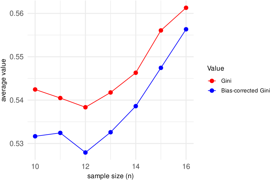
Figure 2: Comparison of standard Gini coefficient ($\widehat{G}$, red line) and bias-corrected Gini ($\widehat{G}_{\text{bc}}$, blue line) for different sample sizes $n$ ($\alpha_{1}=0.5$ and $\alpha_{2}=2.0$).

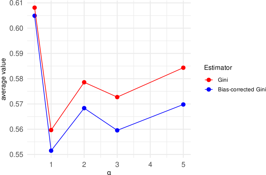
Figure 3: Comparison of standard Gini coefficient ($\widehat{G}$, red line) and bias-corrected Gini ($\widehat{G}_{\text{bc}}$, blue line) for different values of $\alpha_{2}$ ($\alpha_{1}=0.5$ and $n=15$).

6 Concluding remarks

In this paper, we have proposed the bias in the estimation of the Gini coefficient for gamma mixture populations. While the sample Gini coefficient is unbiased for single gamma distributions, we have demonstrated both theoretically and empirically that this property does not hold for gamma mixture models. We have derived a bias expression for the Gini coefficient for gamma mixture populations, which allowed us to propose a bias-corrected Gini estimator. An illustrative Monte Carlo simulation study has been carried out to evaluate the behavior of the bias-corrected Gini estimator. The results emphasized the that the standard Gini coefficient estimator exhibits a consistent upward bias when applied to gamma mixture populations, and the proposed bias correction effectively mitigates this issue, providing a more reliable estimator for gamma mixture distributions. As part of future research, it will be of interest to extend the study to multivariate Gini coefficients. Furthermore, alternative correction methods or the analysis to other mixture models can be developed; see Pérez et al., (1986). Work on these problems is currently in progress and we hope to report these findings in future.

Acknowledgements

The research was supported in part by CNPq and CAPES grants from the Brazilian government.

Disclosure statement

There are no conflicts of interest to disclose.

References

• Abouammoh et al., (2015) Abouammoh, A. M., Alshangiti, A. M., and Ragab, I. E. (2015). A new generalized lindley distribution. Journal of Statistical Computation and Simulation, 85:3662–3678.
• Abramowitz and Stegun, (1972) Abramowitz, M. and Stegun, I. A. (1972). Handbook of Mathematical Functions with Formulas, Graphs, and Mathematical Tables. Dover, New York, 9th printing edition.
• Baydil et al., (2025) Baydil, B., de la Peña, V. H., Zou, H., and Yao, H. (2025). Unbiased estimation of the gini coefficient. Statistics and Probability Letters.
• Botta et al., (1987) Botta, R. F., Harris, C. M., and Marchal, W. G. (1987). Characterizations of generalized hyperexponential distribution functions. Communications in Statistics Stochastic Models, 3:115–148.
• Chotikapanich and Griffiths, (2008) Chotikapanich, D. and Griffiths, W. E. (2008). Estimating Income Distributions Using a Mixture of Gamma Densities, pages 285–302. Springer New York, New York, NY.
• Damgaard and Weiner, (2000) Damgaard, C. and Weiner, J. (2000). Describing inequality in plant size or fecundity. Ecology, 81:1139–1142.
• D’Aurizio, (2016) D’Aurizio, J. (2016). Integrating the lower incomplete gamma $\int_{0}^{\infty}x^{a-1}e^{-sx}\gamma(b,x)\mathrm{d}x$. Mathematics Stack Exchange.
• Deltas, (2003) Deltas, G. (2003). The small-sample bias of the gini coefficient: Results and implications for empirical research. Review of Economics and Statistics, 85:226–234.
• Dorfman, (1979) Dorfman, R. (1979). A formula for the gini coefficient. The Review of Economics and Statistics, 61(1):146–149.
• Fang and Chlamtac, (1999) Fang, Y. and Chlamtac, I. (1999). Teletraffic analysis and mobility modeling of pcs networks. IEEE Transactions on Communications, 47:1062–1072.
• Gini, (1936) Gini, C. (1936). On the measure of concentration with special reference to income and statistics. Colorado College Publication, General Series No. 208, pages 73–79.
• Gómez et al., (2014) Gómez, Y. M., Bolfarine, H., and Gómez, H. W. (2014). A new extension of the exponential distribution. Revista Colombiana de Estadística, 37:25–34.
• Kharazmi et al., (2023) Kharazmi, E., Bordbar, N., and Bordbar, S. (2023). Distribution of nursing workforce in the world using gini coefficient. BMC Nursing, 22:151.
• Kitani et al., (2024) Kitani, M., Murakami, H., and Hashiguchi, H. (2024). Distribution of the sum of gamma mixture random variables. SUT Journal of Mathematics, 60(1):17–37.
• Lindley, (1958) Lindley, D. (1958). Fiducial distributions and bayes’ theorem. Journal of the Royal Statistical Society Series B, 20:102–107.
• McDonald and Jensen, (1979) McDonald, J. B. and Jensen, B. C. (1979). An analysis of some properties of alternative measures of income inequality based on the gamma distribution function. Journal of the American Statistical Association, 74:856–860.
• Pérez et al., (1986) Pérez, R., Caso, C., and Gil, M. (1986). Unbiased estimation of income inequality. Statistical Papers, 27:227–237.
• Salem and Mount, (1974) Salem, A. and Mount, T. (1974). A convenient descriptive model of income distribution: the gamma density. Econometrica, 42:1115–1127.
• Shanker, (2015) Shanker, R. (2015). Shanker distribution and its applications. International Journal of Statistics and Applications, 5:338–348.
• Shanker and Mishra, (2013) Shanker, R. and Mishra, A. (2013). A quasi lindley distribution. African Journal of Mathematics and Computer Science Research, 6:64–71.
• Shanker et al., (2013) Shanker, R., Sharma, S., Shanker, U., and Shanker, R. (2013). Sushila distribution and its application to waiting times data. Opin. Int. J. Bus. Manag., 3:1–11.
• Sun et al., (2010) Sun, T., Zhang, H., Wang, Y., Meng, X., and Wang, C. (2010). The application of environmental gini coefficient (egc) in allocating wastewater discharge permit: The case study of watershed total mass control in tianjin, china. Resources, Conservation and Recycling, 54(9):601–608.
• Vila et al., (2024) Vila, R., Nakano, E., and Saulo, H. (2024). Novel closed-form point estimators for a weighted exponential family derived from likelihood equations. Stat, 13:e723.
• Wolfram Research, (2024) Wolfram Research, I. (2024). Mathematica, Version 14.2. Champaign, IL.
• Yao, (1999) Yao, S. (1999). On the decomposition of gini coefficients by population class and income source: a spreadsheet approach and application. Applied Economics, 31(10):1249–1264.