Two-dimensional transverse-field model with the in-plane anisotropy and Dzyaloshinskii-Moriya interaction: Anisotropy-driven transition
Abstract
The two-dimensional (2D) quantum spin- model with the transverse-field , in-plane-anisotropy , and Dzyaloshinskii-Moriya (DM) interactions was investigated by means of the exact diagonalization method, which enables us to treat the -mediated complex-valued Hermitian matrix elements. According to the preceding real-space renormalization group analysis at , the -driven phase transition occurs generically for in contrast to the 1D model where both - and -induced phases are realized for and , respectively. In this paper, we evaluated the function , namely, the differential of with respect to the concerned energy scale, and from its behavior in proximity to , we observed an evidence of the -driven phase transition; additionally, ’s scaling dimension is estimated from ’s slope. It was also determined how the value of the DM interaction influences the order-disorder phase boundary around the multi-critical point, .
keywords:
05.50.+q 05.10.-a 05.70.Jk 64.60.-i1 Introduction
The one-dimensional model
| (1) |
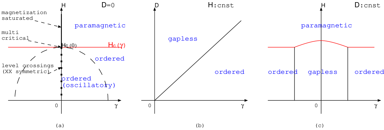
with the transverse field , the in-plane anisotropy , and the spin- operator at site is attracting renewed interest [1, 2, 3] in the context of the quantum information theory [4, 5, 6]. As shown in Fig. 1 (a), a variety of phases appear in the - parameter space [1, 2, 3]. As the transverse field changes, there occurs a phase transition at , which separates the ordered () and paramagnetic () phases. At the isotropic point, , because of the U(1) symmetry, successive level crossings take place [7] up to , whereas for exceedingly large , the magnetization is saturated eventually. Reflecting the level crossings, the ordered phase with oscillatory correlation function extends around the ordinate axis, . Various types of phase boundaries meet at the multi-critical point , and this multi-criticality has been explored in depth [7]. The Dzyaloshinskii-Moriya (DM) interaction changes the phase diagram significantly [8, 9, 10]. For instance, the -induced gapless phase appears for sufficiently large , as shown in Fig. 1 (b). Correspondingly, the - phase diagram for exhibits even richer characters [8, 9]. Actually, as shown in Fig. 1 (c), the phase diagram around the axis is influenced by . The DM interaction alters the magnetization saturation point as
| (2) |
As for the two-dimensional transverse-field model, the - phase diagram for has been investigated both analytically [12, 13] and numerically [13, 14, 15]. In Fig. 2 (a), a schematic - phase diagram obtained with the exact-diagonalization method [13, 14, 15] is shown. The overall features resemble those of the one-dimensional counterpart, Fig. 1 (a); namely, the -driven phase transition between the ordered and paramagnetic phases occurs at . As for the two-dimensional magnet, however, the phase boundary exhibits a “monotonous” [13] increase, as increases. Such a singularity, namely, the multi-criticality at , is characterized by the crossover critical exponent [15]
| (3) |
which describes the end-point singularity of the phase boundary [16, 17] as
| (4) |
The phase boundary rises up linearly, , in two dimensions, whereas for the one-dimensional magnet, the phase boundary takes a constant value, ; see Fig. 1 (a) and 2 (a).
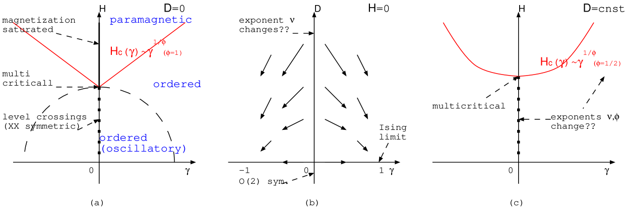
Meanwhile, the DM interaction came under consideration by means of the real-space-renormalization-group method at [18]. As shown In Fig. 2 (b), the Ising limits with are the stable renormalization-group fixed points, and hence, the -driven phase transition occurs for generic values of in sharp contrast to that of the one dimensional counterpart, Fig. 1 (b). Moreover, it was claimed that ’s scaling dimension depends on the DM interaction [18]. To the best of author’s knowledge, such features have not been studied very extensively by other techniques, and the case, which include the multi-criticality, remains totally unclear.
The aim of this paper is to investigate the - phase diagram for the two-dimensional model with (see Fig. 2 (c)). We focus our attention on the -driven criticality so as to examine the real-space-renormalization-group scenario [18] for the extended parameter space. For that purpose, we employed the exact diagonalization method, which enables us to treat the -mediated complex-valued matrix elements. As a probe to detect the phase transition, we evaluated the fidelity susceptibility [4, 7], which is readily accessible via the exact diagonalization scheme. Thereby, we evaluated the fidelity-susceptibility-mediated function, , numerically [19]. From its behavior in proximity to the critical point, , we observed an evidence of the -driven phase transition; we could avoid the complications coming from the level crossings [7] along the axis. It was also determined how the DM interaction alters the multi-criticality.
To be specific, we present the Hamiltonian for the two-dimensional transverse-field model with the DM interaction
| (5) |
Here, the quantum spin- operators are placed at each square-lattice point , and the symbol denotes the unit vectors of the lattice. The parameters, , , , and , denote the ferromagnetic nearest-neighbor interaction, the transverse magnetic field, the in-plane anisotropy, and the DM interaction, respectively; hereafter, the parameter is regarded as the unit of energy, i.e., . Rather technically, we implemented the screw-boundary condition [20, 21, 22] to the finite-size cluster, and the above expression (5) has to be remedied accordingly. The technical details as well as its performance are presented in the next section. The exact diagonalization method enables us to treat the complex-valued Hermitian matrix elements due to the DM interaction; note that the operator has the pure imaginary matrix elements, and the exact diagonalization method is free from the sign problem.
It has to be mentioned that the multi-criticality of the phase boundary has been investigated with the large- expansion method [13] for the -dimensional model with . According to this study, the phase boundary rises up monotonically in large dimensions , whereas the reentrant behavior, namely, a non-monotonic behavior of , is observed in the regime, . Therefore, the case locates around the marginal point , and it is anticipated that ’s multi-criticality would be altered by the perturbations such as the DM interaction.
The rest of this paper is organized as follows. In the next section, the exact numerical results are shown. The above-mentioned screw-boundary condition [20, 21, 22] as well as its performance check are presented in prior to the analysis of the -driven criticality via the function. In the last section, we present the summary and discussions.
2 Numerical results
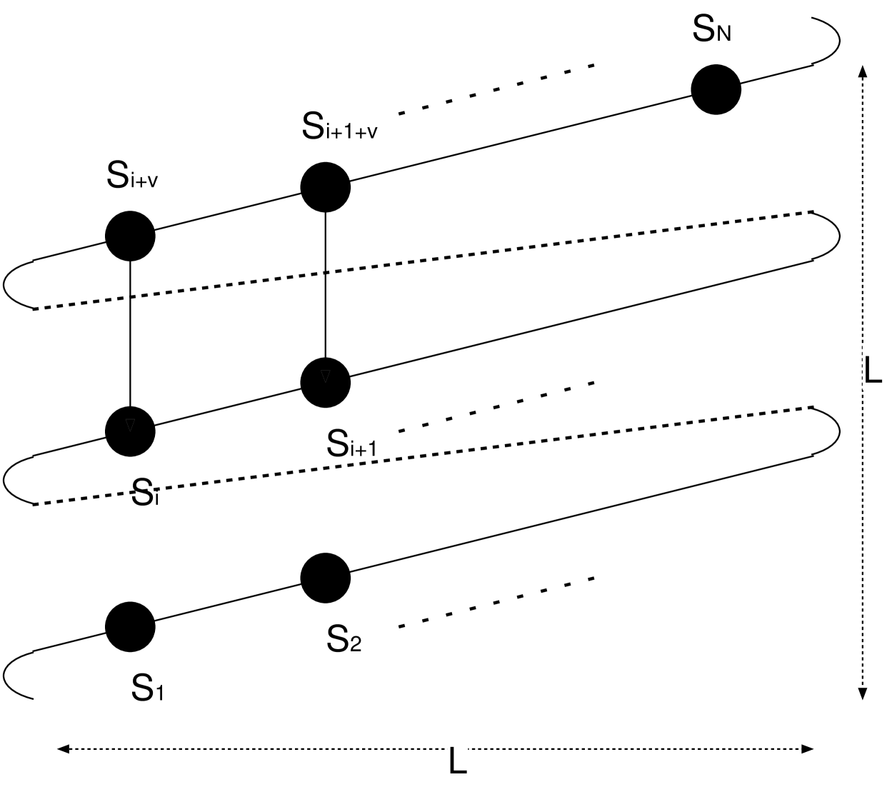
In this section, we present the numerical results for the two-dimensional transverse-field model with the DM interaction. We implemented the screw-boundary condition [20, 21, 22] for the cluster with spins, as shown in Fig. 3. To be specific, the Hamiltonian is given by
| (6) |
for an alignment of spins, with , with the screw pitch, . Here, the bracket takes integer part of a number (Gauss notation), e.g., , and the periodic boundary condition, , is imposed. As shown in Fig. 3, the spins form a sheet of network, and the effective linear dimension of the sheet is given by
| (7) |
The linear dimension plays a significant role in the scaling analyses such as the -driven criticality in Sec. 2.1, where the onset of the Ising universality class is confirmed.
In order to detect the - and -driven phase transitions, we utilized the fidelity susceptibilities [4, 7], and , respectively. To be specific, the former is defined by [4, 7]
| (8) |
with the fidelity (: perturbation field), and the ground state of the Hamiltonian with the magnetic field . Similarly, the latter type was evaluated via
| (9) |
with the fidelity , and the ground state for the in-plane anisotropy . The fidelity susceptibility does not rely on any ad hoc assumptions on the order parameters, i.e., either - () or Ising-symmetric () one, and hence, it is sensitive to generic types of phase transitions.
2.1 Preliminary survey: The -driven order-disorder transition at the Ising case
As a preliminary survey, we investigate the -driven order-disorder phase transition via the fidelity susceptibility (8) at the Ising point, and , where a number of preceding results are available [14, 23]. The criticality belongs to the classical three-dimensional (namely, D) Ising universality class [14, 23].
Before showing the exact numerical results, we recollect a number of scaling relations for (). In general [23], the fidelity susceptibility obeys the scaling formula
| (10) |
with the critical point , and the correlation-length critical exponent . Here, ’s scaling dimension is given by [23]
| (11) |
with the specific-heat critical exponent , and the dynamical critical exponent . Therefore, as for the classical three-dimensional Ising universality class, the scaling dimension takes the value
| (12) |
through resorting to the critical exponents, , [24], and [14, 23]. The critical exponents appearing in the scaling formula (10) are all fixed, and we are able to analyze the order-disorder phase transition via (8).
In Fig. 4, we present the fidelity susceptibility (8) for various and - with the fixed and (Ising limit). The fidelity susceptibility exhibits a notable peak around , which indicates an onset of the phase transition between the ordered () and paramagnetic () phases; see the phase diagram in Fig. 2 (a).
In order to estimate the critical point precisely, in Fig. 5, the approximate critical point is plotted for with the correlation-length critical exponent [14, 23]. The data should align, because the argument of the function in Eq. (10) is a scale-independent constant , which indicates . Here, the parameters, and , are the same as those of Fig. 4. The approximate critical point denotes ’s peak position
| (13) |
for each system size (7). The least-squares fit to these data yields an estimate in the thermodynamic limit . The data in Fig. 5 appear to be convexly curved because of the corrections to the finite-size scaling [25] as well as the screw-boundary condition [26]. Actually, in the screw-boundary condition [26], a wide range of has to be considered, because the wavy deviation between the quadratic , and an intermediate appears, and such an undulation has to be smeared out by including a sector of - at least. On the one hand, as shown in Fig. 8 of Ref. [25], the approximate critical point is curved convexly, and the extrapolated critical point for the largest drifts to a slightly smaller value. In order to appreciate the amount of errors, we made the similar analysis for the largest three system sizes, , which do not contain . As a result, we arrive at an estimate ; the deviation from the above, seems to dominate the least-squares-fit error, ; corrections to scaling appear to be non-negligible. Hence, considering the former as the main source of uncertainty, we estimate the critical point as
| (14) |
Our result (14) appears to agree with the quantum Monte Carlo [23] and exact diagonalization [14] results, confirming the validity of the numerical scheme based on the screw-boundary condition, Eq (6).


As a cross-check, in Fig. 6, we present the scaling plot, -, for various system sizes, -, with (14), [14, 23], and (12), based on the finite-size scaling formula (10). The scaled data fall into the scaling curve satisfactorily, confirming the validity of our exact numerical scheme. We stress that the scaling parameters, , , and , were all fixed in prior to the scaling analysis, and there is no ad hoc adjustable parameter in the analysis of Fig. 6. The scaled peak position in Fig. 6 locates around the off-critical regime, . In the thermodynamic limit , this relation indicates that the peak position converges to the critical point as .

2.2 The -driven criticality for and
In this section, we analyze the -driven phase transition for and (see Fig. 2 (b)) with the aid of the fidelity susceptibility, (9). As mentioned in Introduction, we evaluated the function [19]
| (15) |
with the fidelity susceptibility (9) for the system size , and ’s scaling dimension (11). Formally, the function is defined by the differential of the coupling constant with respect to the concerned energy scale
| (16) |
with the cut-off . This formal expression is well approximated by the above formula (15) [19]. Because the argument of the function in Eq. (10) is a constant , and the inverse of the system size sets the cut-off , the formal expression (16) reduces to
| (17) |
with the correlation-length critical exponent and the transition point, . Therefore, ’s scaling dimension, , is estimated from the slope of in the vicinity of the critical point, . According to the real-space normalization group [18], the -driven transition should take place at
| (18) |
We stress that the asymptote (17) is realized in close vicinity of the critical point, . Actually, the power-law singularity of the critical phenomenon is well defined in proximity to the critical point, and hence, the slope of the function for , namely, the first derivative of around the critical point, captures the concerned critical exponent correctly. The numerical data suffer from the finite-size artifact [7] due to the level crossings along the axis; see Fig. 2 (a). Therefore, from the proximate behavior of the function beside , we observe the critical behavior (particularly, ’s slope, ), avoiding the complications arising from the level crossings at . In order to evaluate the via Eq. (15), we need to fix the the scaling dimension . Putting (: dimensionality) [25] and (same as that of Sec. 2.1) into the scaling relation (11), we obtain
| (19) |
We put this value into the the -function formula (15), and evaluated it by the exact numerical method.
In Fig. 7, we present the function, (15), for various and () , () , and () with the fixed and . We also show the line as a dotted line. The numerical data approach to this line asymptotically for sufficiently small . According to Eq. (17), the slope of this line and the -intercept yield and , respectively. Hence, we estimate the correlation-length critical exponent
| (20) |
and the transition point (18). The critical exponent (20) is identical to that of Fig. 6 of Ref. [27], where the scaling dimension of the symmetry-breaking magnetic field , , and the critical point, , are estimated for the Ising model. Therefore, regarding as the symmetry-breading field in Ref. [27], the underlying physics is the same as ours, and the renormalization-group result (18) [18] is supported by this preceding result [27]. Here, we stress that this idea is retained even in the presence of the DM interaction, because the numerical data in Fig. 7 are almost independent on ; this is not so trivial, as shown in the analysis of the multi-criticality in Sec. 2.4. Moreover, the deviation of the numerically evaluated function from the asymptote was observed in the left panel of Fig. 11 of Ref. [27], where the logarithmic plot for the magnetic susceptibility is shown, and the anticipated slope is realized only within a narrow window beside the critical point . The situation of Ref. [27] is essentially the same as the function, where the logarithmic discrete derivative of is taken as shown in Eq. (15). Hence, substantial improvement of the convergence is only attained by enlarging at a geometrical rate, and such a treatment cannot be managed by the numerical methods. The small- results for are missing because of the following reason. At the rotational symmetric point , the total magnetization commutes with the Hamiltonian, and it takes the quantized values, . Therefore, as the conjugate magnetic field changes, the magnetization shows intermittent jumps because of the successive level crossings; see Fig. 2 (a). Owing to the level crossings, the numerical results in close vicinity of get scattered, and those results are missing in Fig. 7.

We address a number of remarks. First, as shown in Table 1, the case of and has been investigated rather extensively by means of the real-space-renormalization-group method [28, 18]. In Ref. [28], an information-theoretical quantifier, the so-called concurrence , was evaluated, and from ’s peak position , and the peak height , the critical exponent was estimated as and , respectively. Furthermore, the result was obtained from the power-law singularity of the energy gap [18]. The latter is in perfect agreement with ours (20). Second, the case of and has been investigated in Ref. [18]. According to this elaborated study [18], the critical exponent should decrease, as increases. Our exact numerical result indicates that the critical exponent (20) is retained even for the non-zero . Last, we stress that the slope of the function in the vicinity of the critical point makes sense. We recall the correlation-length power-law divergence [29]. From the power-law divergence of , the expression (17) is derived through resorting to the formal definition (16), and .
| method | (probe) | ||
|---|---|---|---|
| RSRG [28] | (), () | ||
| RSRG [18] | (energy gap) | decreases | |
| ED (this work) | (’s slope) |
2.3 The -driven criticality for and
In this section, we investigate the case of and , which is not covered by the preceding studies [28, 18].
In Fig. 8, we present the function, (15), for various , and () , () , and () with . The function seems to obey the asymptotic form, (17), with the slope (20) for sufficiently small , as in the case of (Sec. 2.2). As mentioned in Sec. 2.2, the critical exponent (20) is identical to that of the symmetry-breaking-field-driven criticality as in Ref. [27], regarding the anisotropy as the symmetry breaking field. Hence, the underlying physics is the same as ours, and we stress that the idea is validated even in the presence of as well as . Again, the deviation of the numerically evaluated function from the asymptote should be attributed to the subtlety of the discrete logarithmic derivative of in Eq. (15), as argued in Sec. 2.2. Taking a closer look, we notice that for rather large , the results show a slow convergence to the asymptote . Such a feature for large- regime should be regarded as a precursor of the multi-criticality, which is studied in the next section.
We address a number of remarks. First, according to the renormalization-group analysis for [18], the critical exponent decreases, as increases. In contrast, the present analysis suggests that the critical exponent (20) is robust against the variation of as well as . Last, our results in Sec. 2.2 and 2.3 indicate that the -driven phase transition occurs at (18). Such a feature provides a marked contrast to that of the one-dimensional counterpart (Fig. 1 (c)), where a transient gapless phase is induced by for . A peculiarity of the one-dimensional () model is that the magnetic order develops only marginally (gapless), and in the presence of the DM interaction, the in-plane anisotropy cannot support the magnetic order. On the contrary, in two dimensions, the long-range order develops for the -symmetric () case, and the non-zero term immediately leads to the magnetic order along the easy-axis direction even in the presence of .

2.4 The -driven criticality for large : Multi-criticality for
In this section, we show an evidence that for large (2), the -driven critical exponent becomes
| (21) |
instead of (20) eventually; see Table 1. This result indicates that owing to , the crossover critical exponent changes, and accordingly, the phase boundary (4) becomes curved quadrically, as shown in Fig. 2 (c).
Before commencing the analysis of the multi-critical exponent via , we recollect related multi-critical scaling relations so as to elucidate the implications of (21). The crossover critical exponent (4) is given by [16, 17]
| (22) |
with the - and -driven correlation-length critical exponents, and , respectively, at the multi-critical point (2). As for , we set
| (23) |
which describes the -induced phase transition to the fully-polarized state [30]. Hence, combining this with the aforementioned one, (21), we arrive at
| (24) |
for . This result indicates that the phase boundary should curve quadratically, (4), as mentioned in the first paragraph of this section.
In Fig, 9, we present the function, (15), for various , and () , () , and () with . The function appears to obey the asymptotic form, (17), with the slope (21), as indicated by the dotted line. The deviation of the numerically evaluated function from the asymptote was observed in the right panel of Fig. 11 of Ref. [27], where the logarithmic plot of the susceptibility for the Ising model at the critical end-point is shown, and the anticipated slope is realized only within an extremely narrow window. As shown in Ref. [27], Such an end-point singularity (multi-criticality at is affected by the criticality along the branch ( and ) in a transient manner for finite system sizes, because the former slope is smaller than the latter . Moreover, the (21) is mathematically supported, because this exponent appears in the exact solution for the spin chain (see Fig. 1 (c)); note that the exponent means , which is derived by the rigorous argument. (The fractional (non-integral) value of yields the power-law singularity as to , and such a singularity is not validated by the rigorous argument [13].) Taking a closer look, rather small- data exhibit a slow convergence to the asymptote, suggesting that the term is significant to realize .

We stress that the multi-critical exponent (21) right at differs significantly from (20) for the branch: Actually, as shown in Fig. 9, for sufficiently large () and () , the exact numerical results are almost overlapping with , whereas for rather small () , the data show a slight deviation from the asymptote at least within the available . This deviation should be regarded as a transient behavior, and for sufficiently large , the multi-criticality (21) would be realized for generic nonzero . As mentioned above, the result implies (24) which differs (3) for [15]. Therefore, to the extent of the undertaken parameter space, only the multi-critical exponents, and , are affected by the DM interaction, and the other features are retained unlike the one-dimensional magnet.
3 Summary and discussions
The two-dimensional transverse-field model (5) with the DM interaction was investigated with the exact diagonalization method, which enables us to treat the complex-valued matrix elements due to . We implemented the screw-boundary condition (6) to the finite-size cluster with spins. As a preliminary survey, we analyzed the -driven criticality at the Ising point, and . With the fidelity susceptibility (8), we estimated the critical point as [Eq. (14)], which agrees with the preceding estimates, [23] and [14], confirming that the order-disorder phase transition belongs to the classical three-dimensional-Ising universality class, (12). We then turn to the analysis of the -driven phase transition. In order to cope with the level crossings [7] at , we evaluated the function, (15), and from its slope beside , we obtained an estimate (20) for generic values of and . According to the real-space-renormalization-group analysis for and [28], the estimates, and , were obtained from the peak position and the peak height of (: concurrence), respectively. Likewise, the critical exponent [18] was obtained from the energy gap for and , and it was claimed that the exponent should be a monotonically decreasing function. As mentioned above, our result indicates that the index (20) is robust against and even . It was also determined how the critical exponent changes at the multi-critical point . Our result indicates that the multi-criticality turns into (21) for eventually, and accordingly, the crossover critical exponent changes to (24). Therefore, the DM interaction alters the power-law singularity of the phase boundary, (4), as shown in Fig. 2 (c).
According to the spherical model analysis [13], the phase boundary should exhibit a monotonic increase in large dimensions , whereas a reentrant behavior may occur in . It is thus expected that the multi-criticality is sensitive to the perturbations such as , because the concerned dimensionality locates around the marginal point . In fact, our result indicates that the DM interaction alters the crossover exponent to (24). It is tempting to consider the easy-plane SU magnet [31] with the in-plane anisotropy and the DM interaction to see whether the phase boundary exhibits exotic features such as the reentrant behavior. This problem is left for the future study.
Acknowledgment
This work was supported by a Grant-in-Aid for Scientific Research (C) from Japan Society for the Promotion of Science (Grant No. 20K03767).
References
References
- [1] J. Maziero, H. C. Guzman, L. C. Céleri, M. S. Sarandy, and R. M. Serra, Phys. Rev. A 82 (2010) 012106.
- [2] Z.-Y. Sun, Y.-Y. Wu, J. Xu, H.-L. Huang, B.-F. Zhan, B. Wang, and C.-B. Duanpra, Phys. Rev. A 89 (2014) 022101.
- [3] G. Karpat, B. Çakmak, and F. F. Fanchini, Phys. Rev. B 90 (2014) 104431.
- [4] Q. Luo, J. Zhao, and X. Wang, Phys. Rev. E 98 (2018) 022106.
- [5] A. Steane, Rep. Prog. Phys. 61 (1998) 117.
- [6] C.H. Bennett and D.P. DiVincenzo, Nature 404 (2000) 247.
- [7] V. Mukherjee, A. Polkovnikov, and A. Dutta, Phys. Rev. B 83 (2011) 075118.
- [8] T.-C. Yi, W.-L. You, N. Wu, and A. M. Oleś, Phys. Rev. B 100 (2019) 024423.
- [9] L.-J. Ding and Y. Zhong, Communications in Theoretical Physics 73 (2021) 095701.
- [10] R. Jafari, M. Kargarian, A. Langari, and M. Siahatgar, Phys. Rev. B 78 (2008) 214414.
- [11] F.C. Alcaraz and W.F. Wreszinski, J. Stat. Phys. 58 (1990) 45.
- [12] S. Jalal, R. Khare, and S. Lal, arXiv:1610.09845.
- [13] S. Wald and M. Henkel, J. Stat. Mech.: Theory and Experiment (2015) P07006.
- [14] M. Henkel, J. Phys. A: Mathematical and Theoretical 17 (1984) L795.
- [15] Y. Nishiyama, Eur. Phys. J. B 92 (2019) 167.
- [16] E.K. Riedel and F. Wegner, Z. Phys. 225 (1969) 195.
- [17] P. Pfeuty, D. Jasnow, and M. E. Fisher, Phys. Rev. B 10 (1974) 2088.
- [18] T. Farajollahpour and S. A. Jafari, Phys. Rev. B 98 (2018) 085136.
- [19] H.H. Roomany and H.W. Wyld, Phys. Rev. D 21, 3341 (1980).
- [20] M. Nakamura, S. Masuda, and S. Nishimoto, Phys. Rev. B 104 (2021) L121114.
- [21] Y. Nishiyama, Phys. Rev. B 79 (2009) 054425.
- [22] A. Miyata, T. Hikihara, S. Furukawa, R. K. Kremer, S. Zherlitsyn, and J. Wosnitza, Phys. Rev. B 103 (2021) 014411.
- [23] A. F. Albuquerque, F. Alet, C. Sire, and S. Capponi, Phys. Rev. B 81 (2019) 064418.
- [24] M. Campostrini, A. Pelissetto, P. Rossi, and E. Vicari, Phys. Rev. E 65 (2002) 066127.
- [25] M. S. S. Challa, D. P. Landau, and K. Binder, Phys. Rev. B 34 (1986) 1841.
- [26] M. A. Novotny, J. Appl. Phys. 67 (1990) 5448.
- [27] K. Binder and D. P. Landau, Phys. Rev. B 30 (1984) 1477.
- [28] M. Usman, A. Ilyas, and K. Khan, Phys. Rev. A 92 (2015) 032327.
- [29] M. Vojta, Rep. Prog. Phys. 66 (2003) 2069.
- [30] V. Zapf, M. Jaime, and C. D. Batista, Rev. Mod. Phys. 86 (2014) 563.
- [31] J. D’Emidio and R. K. Kaul, Phys. Rev. B 93 (2016) 054406.