Implicit Generative Modeling by Kernel Similarity Matching

Abstract

Understanding how the brain encodes stimuli has been a fundamental problem in computational neuroscience. Insights into this problem have led to the design and development of artificial neural networks that learn representations by incorporating brain-like learning abilities. Recently, learning representations by capturing similarity between input samples has been studied (Pehlevan et al., 2018) to tackle this problem. This approach, however, has thus far been used to only learn downstream features from an input and has not been studied in the context of a generative paradigm, where one can map the representations back to the input space, incorporating not only bottom-up interactions (stimuli $\to$ latent) but also learning features in a top-down manner (latent $\to$ stimuli). We investigate a kernel similarity matching framework for generative modeling. Starting with a modified sparse coding objective for learning representations proposed in prior work (Olshausen and Field, 1996a; Tolooshams and Ba, 2021)), we demonstrate that representation learning in this context is equivalent to maximizing similarity between the input kernel and a latent kernel. We show that an implicit generative model arises from learning the kernel structure in the latent space and show how the framework can be adapted to learn manifold structures, potentially providing insights as to how task representations can be encoded in the brain. To solve the objective, we propose a novel Alternate Direction Method of Multipliers (ADMM) based algorithm and discuss the interpretation of the optimization process. Finally, we discuss how this representation learning problem can lead towards a biologically plausible architecture to learn the model parameters that ties together representation learning using similarity matching (a bottom-up approach) with predictive coding (a top-down approach).

1 Introduction

Learning meaningful representations from data is one of the fundamental goals in engineering applications and scientific discovery. In the field of machine learning, extracting high-quality representations from input data has empowered algorithms to significantly improve their performance on any given task. In neuroscience, the challenge of developing algorithms that can learn representations useful for downstream tasks while respecting the biological constraints of learning is of particular interest, as it may potentially shed light on the neural basis of behavior. Recent approaches in both fields have focused on learning such representations by capturing the relationship between different samples and ensuring that a similar association is maintained within the learned representations. By comparing samples with one another, such unsupervised approaches can help in learning robust representations for downstream tasks.

In classical machine learning literature, unsupervised methods – like Isomap, Multi-dimensional Scaling, t-SNE – have long been used to learn good representations by measuring some notion of similarity, such as distance, kernel structure etc. between input samples (Cox and Cox, 2000; Choi and Choi, 2004; Van der Maaten and Hinton, 2008; Ghodsi, 2006). More recently, similarity based representation learning have been explored in the context of deep learning techniques, such as contrastive learning and graph neural nets (Chen et al., 2020; Zimmermann et al., 2021; Sanchez-Lengeling et al., 2021). In neuroscience, recent work by (Pehlevan et al., 2018; Luther and Seung, 2022) adapt these similarity based techniques to develop biologically plausible models for representation learning, providing mechanistic understanding about how neurons in the brain may encode external stimuli. However, while these similarity-based measures are effective for feature extraction, they typically lack a mapping back to the input space, which limits their ability to capture tow-down interactions critical for sensory processing,(Keller and Mrsic-Flogel, 2018; Boutin et al., 2021; Rao and Ballard, 1999). Achieving this would require a generative approach, which would allow higher cortical layers interact with and modulate lower layers as they process the input stimuli. For instance, (Boutin et al., 2021) demonstrated in their work that such interactions are useful for explaining important features of neural processing in the visual cortex, such as contour integration, accounting for object perception in the V1 layer even with degraded images, this shedding light into how we perceive visual stimuli based on expectations and implicit world knowledge, rather than just raw sensory input. Furthermore, the top-down interactions also play a critical role in regulating information flow from incoming sensory data, ensuring only essential information gets propagated to higher cortical areas, thereby reducing redundancy (Keller and Mrsic-Flogel, 2018). These studies indicate that integrating top-down interactions in the representation learning process is essential for understanding how the brain encodes and interprets sensory information.

Figure 1: (a) Kernel Similarity Matching (KSM) approaches have been successfully used previously in the context of unsupervised representation learning which only warrants learning a bottom-up map from the input to the representations. Prior works have utilized this framework in formulating dimensionality reduction techniques such as IsoMap, Multi-Dimensional Scaling (MDS) (Ghodsi, 2006) and t-SNE (Van der Maaten and Hinton, 2008), in addition to developing neurally plausible models for the same. (c) Generative models, on the other hand involves a bi-directional learning process where the learned representations need to map back to the input space, requiring a top-down map. (b) We propose that KSM frameworks can serve as link to extend unsupervised feature learning to generative models. We leverage one class of generative models rooted in dictionary learning methods (Kreutz-Delgado et al., 2003) to extend kernel matching objectives to a generative framework learning objective where the representations not only have to predict the input data but also have to satisfy sparsity constraints. The learning in these cases occur through a combination of both bottom-up (to estimate latent) and top-down (to predict input using the latents) interaction.

We examine the representation learning problem in the context of sparse dictionary learning (Olshausen and Field, 1997). Sparse dictionary learning refers to a class of generative models that have been widely used in the field of signal processing, machine learning and neuroscience to obtain parsimonious representations of the input data, at the same time learning a dictionary of atoms that map the learned representations back to the input space. Mathematically, the problem can be defined as:

$$\underset{{\bm{A}},{\bm{Z}}}{\min}\,\,\frac{1}{2T}\|{\bm{X}}-{\bm{A}}{\bm{Z}}\|_{F}^{2}+\frac{\lambda}{T}\|{\bm{Z}}\|_{1,1}$$ (1)

$$\text{s.t.}\,\,\|{{\bm{a}}}_{i}\|_{2}\leq 1,\forall i\in\{1,\dots,K\}$$

where, $\|\cdot\|_{1,1}$ denotes the sum of absolute values of the elements of the matrix, ${\bm{X}}$ is the input data matrix ($\in{\mathbb{R}}^{N\times T})$, ${\bm{Z}}$ is the matrix of sparse codes, also called latent representations $(\in{\mathbb{R}}^{K\times T})$ respectively, with $T$ being the number of independent examples, $\lambda$ is the sparsity parameter and ${\bm{A}}$ is the dictionary ($\in{\mathbb{R}}^{N\times K})$, which maps the latent back to the input space. Such models have been used to explain receptive field structure and the neuronal activity in the V1 cortex. (Olshausen and Field, 1996b, 1997).

While sparse dictionary learning has been used to explain the emergence of receptive fields in the V1 region of the visual cortex, predictive coding approaches provide another perspective on theory of cortical processing. Built upon the concept of sparse dictionary learning, predictive coding theory extends it to incorporate hierarchical systems in which only the essential information is propagated upwards from downstream layers, providing an efficient coding mechanism. This is achieved by prediction errors from higher(top) cortical layers of the activity in the lower(down) cortical layers, analogous to the goal of minimizing the reconstruction loss in sparse dictionary learning. Originally explored in the context of providing a theory for retinal and LGN cells by (Mumford, 1992), applications of predictive coding theory to cortical functions was later extended by (Rao and Ballard, 1999), who used it to explain sensory interactions in the visual cortex. Recent works by (Boutin et al., 2021) have focused on integrating sparse dictionary learning with predictive coding to model hierarchical processing in both V1 and V2 areas of the visual cortex, while (Rao, 2024) use predictive coding approaches to propose a unified theory for sensory and motor processes across the neocortex. As a result, predictive coding methods offer a promising framework for developing models that incorporate top-down interactions in the representation learning process.

In this work, we investigate how similarity based representation learning can be adapted to a generative paradigm.

• Our first contribution is to show an equivalence between similarity based approaches and sparse dictionary learning. We argue that alongside learning representations, learning the kernel structure in the representation space itself can lead to an implicit generative map between the input and the corresponding representations.

• Our second contribution demonstrates the flexibility of our framework towards learning diverse generative maps, in particular, manifold structures. We achieve this by modifying the constraints on the learned representations and the kernel structure itself.

• Third, we develop a novel formulation of an Alternate Direction Method of Multipliers (ADMM) (Boyd et al., 2011)) to derive the update dynamics for the variables involved in the optimization process.

• Finally, we lay the foundations towards a biologically plausible framework for our proposed model, where representation learning is facilitated by combining both combining similarity based approaches with a predictive coding framework capturing both top-down and bottom-up interactions.

We begin the rest of our treatment with a brief overview of classical similarity matching techniques, highlighting their role in developing neurally plausible models for representation learning. Section 3 introduces and extends the kernel similarity matching (KSM) framework discussed previously to generative models. In Section 4, we explore how different priors affect representation learning under this framework, focusing on a prior inspired by metabolic constraints on neural activity. Section 5 outlines the general optimization procedure for solving the KSM objective and discusses the computational considerations involved in the gradient dynamics of each optimization variable. We then present observations and insights from numerical experiments applying the proposed frameworks to synthetic and real-world datasets. In Section 7, we take a step toward developing a neurally plausible model for representation learning. We propose a relaxed version of the KSM objective that incorporates both bottom-up and top-down interactions between neurons while enforcing local learning rules for synaptic parameters. We conclude in Section 8 by discussing the approach’s limitations and outlining future directions for contributions.

2 Classical Kernel Similarity Matching for Representation Learning

We start with a brief review of classical kernel similarity matching approaches, which have been explored in the context of developing neurally plausible architectures in recent works (Pehlevan et al., 2018; Luther and Seung, 2022). As discussed in the previous section, such a framework also underpins the extraction of meaningful representations for downstream tasks in many deep unsupervised learning architectures.

Problem formulation. Mathematically, similarity based approaches to representation learning can be described as follows:

$$\underset{{\bm{Z}}\in{\mathcal{C}}}{\max}\,\,d({\mathcal{K}}_{\bm{X}},{\mathcal{K}}_{\bm{Z}})$$ (2)

where, ${\bm{X}}\in{\mathbb{R}}^{N\times T}$ denotes the input data matrix (with $T$ samples each of dimension $N$) and ${\bm{Z}}\in{\mathbb{R}}^{K\times T}$ denotes the corresponding representation matrix (each of dimension $K$). ${\mathcal{C}}$ denotes the set of constraints imposed on the representation space. Here ${\mathcal{K}}_{\bm{X}}$ and ${\mathcal{K}}_{\bm{Z}}$ are called input and representation kernels respectively, which capture the notion of similarity between different samples in the dataset. More generally, for a given data or representation matrix ${\bm{Q}}\in{\mathbb{R}}^{N\times N}$ we can define ${\mathcal{K}}_{\bm{Q}}(s,t)=f_{\bm{Q}}({\bm{q}}_{s},{\bm{q}}_{t})\,\,\forall\,\,s,t\in\{1,2,\dots T\}$ where $f_{\bm{Q}}:{\mathbb{R}}^{N}\times{\mathbb{R}}^{N}\to{\mathbb{R}}$ is the similarity measure between two samples ${\bm{q}}_{s}$ and ${\bm{q}}_{t}$ in ${\mathbb{R}}^{N}$. A simple example for such a mapping could be $K_{Q}(s,t)={\bm{q}}_{s}^{T}\mathbf{Q}{\bm{q}}_{t}$, which is a generalized inner product between ${\bm{q}}_{s}$ and ${\bm{q}}_{t}$, where ${\bm{Q}}\succ 0$ is a positive definite matrix. If ${\bm{Q}}={\bm{I}}$, we have the standard inner product. The function $d$, in Equation 2, denotes a notion of distance (need not be a strict metric) between these two kernels. Common examples for such distance measures could include the vector norms, or arccosine of the inner products. The goal of the optimization problem in Equation 2 being to find representations ${\bm{Z}}$ which makes the input and the representation kernel similar. (Pehlevan et al., 2018) use a standard inner product formulation of the kernel function $f$ given by $f({\bm{x}}_{s},{\bm{x}}_{t})={\bm{x}}_{s}\cdot{\bm{x}}_{t}$, which leads to the classical kernel similarity matching problem for representation learning as given below:

$$\underset{{\bm{Z}}\in{\mathbb{R}}^{K\times T}}{\min}\frac{1}{T^{2}}\|{\bm{X}}^{T}{\bm{X}}-{\bm{Z}}^{T}{\bm{Z}}\|_{F}^{2} =\underset{{\bm{Z}}\in{\mathbb{R}}^{K\times T}}{\min}\frac{1}{T^{2}}\sum\limits_{s,t}\|{\bm{x}}_{s}^{T}{\bm{x}}_{t}-{\bm{z}}_{s}^{T}{\bm{z}}_{t}\|^{2}\noindent$$ (3)

$$=\underset{{\bm{Z}}\in{\mathbb{R}}^{K\times T}}{\min}\frac{1}{T^{2}}\left[-2\operatorname{Tr}({\bm{X}}^{T}{\bm{X}}{\bm{Z}}^{T}{\bm{Z}})+\operatorname{Tr}({\bm{Z}}^{T}{\bm{Z}}{\bm{Z}}^{T}{\bm{Z}})\right]$$

where the final equation comes from the fact that for any matrix ${\bm{G}}$, $\|{\bm{G}}\|_{F}^{2}=\operatorname{Tr}({\bm{G}}^{T}{\bm{G}})$.

An online formulation to tackle computational bottleneck and improve biological feasibility. A key bottleneck with the above formulation is that the objective scales poorly with the size of the dataset as one needs to compute the kernel matrices ${\mathcal{K}}_{\bm{X}}={\bm{X}}^{T}{\bm{X}}$ and ${\mathcal{K}}_{\bm{Z}}={\bm{Z}}^{T}{\bm{Z}}$ over pairs of examples for the entire dataset scaling the computation as ${\mathcal{O}}(T^{2})$. To overcome this (Pehlevan et al., 2018) employed a Legendre transformation rewriting:

$$-\frac{1}{T^{2}}\operatorname{Tr}({\bm{X}}^{T}{\bm{X}}{\bm{Z}}^{T}{\bm{Z}}) \to\underset{{\bm{W}}}{\min}\,-\frac{2}{T}({\bm{X}}^{T}{\bm{W}}^{T}{\bm{Z}})+\operatorname{Tr}({\bm{W}}^{T}{\bm{W}})=-\frac{2}{T}\sum\limits_{t}{\bm{x}}_{t}^{T}{\bm{W}}{\bm{z}}_{t}+\operatorname{Tr}({\bm{W}}^{T}{\bm{W}})$$ (4)

$$\frac{1}{T^{2}}\operatorname{Tr}({\bm{Z}}^{T}{\bm{Z}}{\bm{Z}}^{T}{\bm{Z}}) \to\underset{{\bm{M}}}{\max}\,\frac{2}{T}\operatorname{Tr}({\bm{Z}}^{T}{\bm{M}}{\bm{Z}})-\operatorname{Tr}({\bm{M}}^{T}{\bm{M}})=\frac{1}{T}\sum\limits_{t}{\bm{z}}_{t}^{T}{\bm{M}}{\bm{z}}_{t}+\operatorname{Tr}({\bm{M}}^{T}{\bm{M}})$$

leading to the following min-max problem:

$$\underset{{\bm{Z}}\in{\mathbb{R}}^{K\times T}}{\min}\frac{1}{T^{2}}\|{\bm{X}}^{T}{\bm{X}}-{\bm{Z}}^{T}{\bm{Z}}\|_{F}^{2}=\underset{{\bm{z}}_{t}}{\min}\,\underset{{\bm{W}}}{\min}\,\underset{{\bm{M}}}{\max}\,\,\frac{1}{T}\sum\limits_{t}(-4{\bm{x}}_{t}^{T}{\bm{W}}{\bm{z}}_{t}+2{\bm{z}}_{t}^{T}{\bm{M}}{\bm{z}}_{t})+2\operatorname{Tr}({\bm{W}}^{T}{\bm{W}})-\operatorname{Tr}({\bm{M}}^{T}{\bm{M}})$$ (5)

The key takeaway from the discussion above is that employing Legendre transformation allows for the optimization problem to be decoupled over individual samples. While we obtain an increased parameter count by introducing ${\bm{W}}$ and ${\bm{M}}$, the computation of the objective now scales linearly with the size of the dataset. This is also a crucial step towards biologically plausible representation learning which necessitates that neural representations are encoded in an online manner over individual samples (Chklovskii, 2016).

Extensions and limitations. In (Luther and Seung, 2022), the authors extend this framework to a more general kernel structure for $f$ in the input space (${\bm{X}}$) while using the standard inner product kernel for the latent space (${\bm{Z}}$). However, these formulations of the kernel matching objective, typically encode representations in a bottom-up manner (from lower to higher levels) only, neglecting any feedback from higher to lower levels. As a result, they lack top-down interactions that map the representations back to the input space, a key aspect suggested by prevalent theories of cortical processing which view perception as a controlled hallucination where the implicit model that the brain uses is corrected by feedback of the sensory prediction error (Deneve and Jardri, 2016; Millidge et al., 2021). In the next section we articulate how these similarity based approaches can be extended to learn representations from the input as well as learning an implicit generative map that links them back to the input space.

3 Kernel Similarity Matching (KSM) as implicit generative models

To extend the kernel matching framework for generative models, we focus on dictionary learning methods, where representations are learned by minimizing the prediction error with respect to the input while having some form of constraints on the latent space and show an equivalence between the two.

A similarity-matching formulation of sparse dictionary learning. We begin with a modified version of the sparse dictionary learning objective (described in Equation 1), which incorporates the norm constraints on the dictionary columns directly into the objective itself as demonstrated in (Lee et al., 2006; Tolooshams and Ba, 2022). From an optimization standpoint, the norm constraints on the dictionary columns solve the scaling ambiguity in of the objective in Equation 1 where the sparse representations and the dictionary columns can be scaled arbitrarily while maintaining the same reconstruction loss. This improves the stability and convergence of the optimization approaches on a variety of sparse dictionary learning based models (Jiang and de la Iglesia, 2021). From a neuroscience perspective, normalized dictionary columns ensures that the learned codes have a consistent scale of contribution towards encoding the input, with the magnitude of contribution directly influenced by the amplitude of the corresponding code. This facilitates better interpretability when analyzing population activity across different regions of the brain (Tolooshams et al., 2024). Furthermore, normalization of dictionary columns aligns with the concept of synaptic normalization (Turrigiano and Nelson, 2004; Mayzel and Schneidman, 2023) in neuroscience, where an increase (decrease) of a particular synaptic weight, increases (decreases) the strength of other synapses in the network, leading to a more biologically realistic theory of networks encoding neural population codes. The modified sparse coding objective given below incorporates the norm constraints on the dictionary columns as a penalty or regularizer in the objective itself which leads to the revised optimization problem:

$$P_{1}:\underset{{\bm{A}},{\bm{Z}}}{\min}\,\,\frac{1}{2T}\|{\bm{X}}-{\bm{A}}{\bm{Z}}\|^{2}_{F}+\frac{\lambda}{T}\|{\bm{Z}}\|_{1,1}+\frac{\omega}{2}\|{\bm{A}}\|_{F}^{2}\qquad\omega>0$$ (6)

Here, $\|{\bm{Z}}\|_{1,1}=\sum\limits_{i,j}|z_{ij}|$.

The objective in Equation 6 is a bilevel optimization problem which is traditionally solved in literature (Olshausen and Field, 1996a), (Dempe and Zemkoho, 2020), (Zhang et al., 2024) through alternating minimization, where one solves the objective first w.r.t. to the latent representation ${\bm{Z}}$ (inner optimization problem) while fixing ${\bm{A}}$ to obtain the optimum ${\bm{Z}}^{*}$. Thereafter, fixing ${\bm{Z}}$ to ${\bm{Z}}^{*}$, we solve the objective w.r.t. ${\bm{A}}$ (outer optimization problem), and repeat these two steps until convergence. To see the connection to kernel similarity matching, we make use of the Lemma below on the bilevel objective function. We include the proof of the lemma in the appendix for completeness.

Lemma 1 (Min-Min Lemma).

Let $f({\bm{x}},{\bm{y}})$ be a function with finite minima where ${\bm{x}}\in{\mathbb{R}}^{m}$ and ${\bm{y}}\in{\mathbb{R}}^{n}$ for $m,n\in{\mathbb{N}}$ respectively, then the following holds:

$$\underset{{\bm{x}}}{\min}\,\,\underset{{\bm{y}}}{\min}\,\,f({\bm{x}},{\bm{y}})=\underset{{\bm{y}}}{\min}\,\,\underset{{\bm{x}}}{\min}\,\,f({\bm{x}},{\bm{y}})$$

Proof.

See Appendix A ∎

Essentially, Lemma 1 allows us to switch the order of optimization in a bilevel optimization problem. Consequently, our inner optimization problem in Equation 6 now becomes w.r.t. ${\bm{A}}$ followed by ${\bm{Z}}$ for the outer optimization. This leads to the following proposition:

Proposition 1.1.

Let $P_{1}$ be the sparse dictionary learning problem as described above and $Q_{1}$ be the formulation as described below:

$$Q_{1}:\underset{{\bm{Z}},{\bm{H}}}{\min} -\frac{1}{2T^{2}}\operatorname{Tr}(\underbrace{{\bm{X}}^{T}{\bm{X}}}_{{\mathcal{K}}_{{\bm{X}}}}\underbrace{{\bm{Z}}^{T}{\bm{H}}^{-1}{\bm{Z}}}_{{\mathcal{K}}_{{\bm{Z}}}})+\frac{\lambda}{T}\|{\bm{Z}}\|_{1,1}$$ (7)

s.t. $${\bm{H}}=\frac{{\bm{Z}}{\bm{Z}}^{T}}{T}+\omega{\bm{I}}$$

then from lemma 1 we have $P_{1}$ and $Q_{1}$ are equivalent.

Proof.

See Appendix A.1 ∎

Deconstructing the objective. The objective in Equation 7 consists of a trace term and a $L_{1}$ norm regularizer for imposing sparsity on the representations. Additionally, a correlation constraint is enforced on the representations by the matrix ${\bm{H}}$. The trace term represents the matrix inner product between a standard linear input kernel ${\mathcal{K}}_{\bm{X}}={\bm{X}}^{T}{\bm{X}}$ and a modified representation kernel ${\mathcal{K}}_{\bm{Z}}={\bm{Z}}^{T}{\bm{H}}^{-1}{\bm{Z}}$, where the structure of the representation kernel is governed by the matrix ${\bm{H}}$, rather ${\bm{H}}^{-1}$. Notably, if ${\bm{H}}={\bm{I}}$ then we are back to the standard inner product kernel in the representation space (given by ${\bm{Z}}^{T}{\bm{Z}}$).

To gain some intuition about the latent kernel function ${\mathcal{K}}_{\bm{Z}}$ and the corresponding structure matrix ${\bm{H}}^{-1}$, we observe that the matrix ${\bm{H}}$ as defined by the constraint in Equation 7 mimics the sample covariance of the learned representations. Therefore, the transformation ${\bm{H}}^{-\frac{1}{2}}{\bm{Z}}$, essentially de-correlates the latent representation ${\bm{Z}}$, and ${\bm{K}}_{\bm{Z}}$ computes the kernel value in this decorrelated latent space. In essence, the trace term, which denotes the matrix inner product between ${\mathcal{K}}_{\bm{X}}$ and ${\mathcal{K}}_{\bm{Z}}$, captures the similarity measure between the input kernel and the representation kernel. Minimizing the objective in Equation 7 is equivalent to maximizing the trace inner product subject the sparsity and correlation constraints defined in the problem. This, in turn, implies making the input and the representation kernels similar. Juxtaposing Equation 7 with the similarity based representation learning described in Equation 2, we observe that the sparse dictionary learning objective (Equation 6) is equivalent to kernel matching representation learning problem, with an imposed structural constraint on the representation kernel.

This formulation of kernel matching differs from prior similarity-based approaches in one key aspect. In prior methods (Pehlevan et al., 2018; Luther and Seung, 2022), the representation kernel involved in the similarity matching objective was typically restricted to a standard inner product-based formulation. In contrast, the representation kernel in this case is derived from a generalized inner product formulation with the structure of the inner product governed by the matrix ${\bm{H}}^{-1}$, which itself is being estimated through a constraint in the optimization problem, allowing the entire kernel structure to evolve as the representations ${\bm{Z}}$ are being learned. We argue that it is this flexibility in the kernel structure that allows us to formulate an implicit generative map, tying the representations back to the input space.

An implicit generative map. As discussed earlier, the kernel matching objective presented in Equation 7 learns representations ${\bm{Z}}$ corresponding to the input samples ${\bm{X}}$ by aligning the input and the representation kernel. This also allows us to calculate an implicit generative map from the representation space to the input space by estimating the dictionary $\hat{{\bm{A}}}$, where, $\hat{{\bm{A}}}=\dfrac{{\bm{X}}{\bm{Z}}^{T}{\bm{H}}^{-1}}{T}$ (See Appendix A.1 for the proof of this relation). The model prediction $\hat{{\bm{x}}}$ for the corresponding input ${\bm{x}}$ can then be calculated as $\hat{{\bm{x}}}=\hat{{\bm{A}}}{\bm{z}}$, where ${\bm{z}}$ is the representation of ${\bm{x}}$ in the latent space with the final expression for $\hat{{\bm{x}}}$ being given as $\hat{{\bm{x}}}=\dfrac{{\bm{X}}{\bm{Z}}^{T}{\bm{H}}^{-1}}{T}{\bm{z}}=\dfrac{1}{T}\sum\limits_{i=1}^{T}{\bm{x}}_{i}\langle{\bm{z}}_{i},{\bm{z}}\rangle_{{\bm{H}}^{-1}}$, where $\langle\cdot,\cdot\rangle_{{\bm{H}}^{-1}}$ computes the representation kernel between ${\bm{z}}_{i}$ and ${\bm{z}}$, with the structure of the kernel being determined by ${\bm{H}}^{-1}$.

4 A flexible framework with different priors

The representation learning problem articulated in Equation 2 provides a flexible framework that varies depending on the prior imposed on the latent space. Specifically, in the previous section we discussed how imposing the sparsity constraint (using the $L_{1}$ norm) on the latent space alongside the correlation constraint on the representation kernel ${\bm{H}}$ is equivalent to a sparse dictionary learning problem. Additionally, other sparsity based priors (Bach et al., 2012) on the latent representations that do not involve expicit equality constraints also amount to the same formulation as discussed before. It is worth noting that the correlation constraint on the representation kernel ${\bm{H}}$ is a consequence of introducing a norm constraint (an $L_{2}$ prior) on the columns of the dictionary (${\bm{A}}$) and the reconstruction loss, as mentioned in Equation 6, which in turn leads to Proposition 1.1. In this section, we explore how the optimization problem in Equation 7 can be extended to other forms of $L_{2}$ like priors on the dictionary columns which can lead to different behaviors.

A probability simplex prior. We focus our discussion on an interesting case where the representations are constrained on a probability simplex, i.e. each dimension is non-negative and sum across all the dimensions are constrained to unity. From a probabilistic perspective, this corresponds to imposing a dirichlet prior on the representations.

Why this prior? Our choice of this prior is motivated by metabolic constraints in a biological system. In neuroscience, imposing the sparsity constraint is desirable for representation learning as it is tied to minimizing wiring length (Foldiak, 2003) and metabolic efficiency for neural activity (Baddeley, 1996), with the latter arguing the fixing the mean firing rate leads to sparsity in the representations. While the $L_{1}$ norm constraint imposes sparsity, it does not strictly limit the amplitude of each of the desired representations. Imposing sparsity while at the same time limiting the amplitude of the representations can be a more desirable way of imposing metabolic constraints from a biological perspective, as it imposes competition in the population by forcing activity of each neuron (which corresponds to a latent dimension) is bounded, and is undergoes subtractive normalization by the total population activity (i.e. each of the dimensions add upto unity). The idea of normalization of individual neuronal responses by the population response has been formulated as a canonical form of neural computation in different sensory inputs (Carandini and Heeger, 2012; Chalk et al., 2017) across different species. (Carandini and Heeger, 2012) suggest that this kind of computation plays a role in making neural responses more invariant to stimulus properties like contrast or intensity, while at the same time reducing redundancy in the learned representations, whereas (Chalk et al., 2017) argue that the type of normalization is an inherent feature of the kind of noise associated with the generated response to the input stimulus. For our case, the simplex prior, introduces a subtractive normalization effect on neuronal responses where the inhibition in individual activity is additive in nature and governed by the sum of the population activity (See Appendix B for details).

To investigate such a prior on the latent, we start with a dictionary learning objective proposed in a prior work by (Tasissa et al., 2023), where the alongside the representations being constrained on a probability simplex, the proximity of the dictionary columns to the data points is also emphasized in addition to the reconstruction loss. The optimization objective for this case can then be articulated as follows:

$$P_{2}:\underset{{\bm{A}},{\bm{Z}}}{\min} \,\,\frac{1}{2T}\|{\bm{X}}-{\bm{A}}{\bm{Z}}\|_{F}^{2}+\frac{\omega}{T}\sum\limits_{k=1}^{K}\sum\limits_{l=1}^{T}z_{kl}\|{\bm{x}}_{l}-{\bm{a}}_{k}\|_{2}^{2}$$ (8)

s.t. $$\sum\limits_{k=1}^{K}z_{kl}=1,\,\,z_{kl}\geq 0,\quad\forall\quad l\,\in\,\{1,2,\dots,T\}$$

Deconstructing the regularizer. The regularizer here plays an important role in ensuring only dictionary columns ${\bm{a}}_{j}$ that are close to the input sample ${\bm{x}}_{i}$ are utilized in minimizing the reconstruction error (as when $z_{kl}$ is high ${\bm{a}}_{k}$ needs to be close to ${\bm{x}}_{l}$ to minimize the penalty). Additionally, as the representations lie on a probability simplex, the predicted samples by the model lie within the convex hull of the dictionary columns. As a result the objective in Equation 8 is able to piece-wise tile the manifold of the input data with convex polygons, with the dictionary columns ${\bm{a}}_{j}$ serving as anchor points or vertices of these convex polygons (Tasissa et al., 2023). Consequently, these dictionary columns serve as localized receptive fields tiling the surface of the input manifold, with neuronal activity tuned to the location of the receptive fields along the manifold surface. This can be helpful in understanding how a neural manifold can be decoded by downstream system for different task characteristics (Jazayeri and Ostojic, 2021; Chung and Abbott, 2021). For instance, spatially localized response is a key mechanism by which hippocampus place cell facilitate navigation (O’Keefe, 1978). In addition, head direction circuits in fly also involve localized receptive fields that are oriented to the angle where the head is pointing towards (Chaudhuri et al., 2019). Other works have also explored the role localized receptive fields play in understanding input features such as object and orientation selectivity in the visual cortex (Hubel et al., 1959; Chung and Abbott, 2021) and frequency selectivity in the auditory cortex (Knudsen and Konishi, 1978; Da Costa et al., 2013).

In later sections, we show that imposing such simplex based constraints as shown in Equation 9 not only allows us to learn localized receptive fields along the surface of the manifold, but togther with the estimatated latent representations, piece-wise approximate the input data manifold, with the localized receptive fields serving as anchors on the input manifold, and the latent representations modeling population activity tuned to these receptive fields over different sections of the input manifold.

Kernel Similarity Matching (KSM) for Manifold Learning. We note that the objective in Equation 8 is again a bilevel optimization problem in ${\bm{A}}$ and ${\bm{Z}}$. Therefore, we once again employ lemma 1 to switch the order of optimization which leads to the following proposition:

Proposition 1.2.

Let $P_{2}$ be the optimization problem as described before and $Q_{2}$ be the formulation as described below:

$$Q_{2}:\underset{{\bm{Z}},{\bm{H}}}{\min} -\frac{1}{2T^{2}}\operatorname{Tr}({\bm{X}}^{T}{\bm{X}}{\bm{Z}}^{T}{\bm{H}}^{-1}{\bm{Z}})$$ (9)

s.t. $$\,\,{\bm{Z}}^{T}\mathbf{1}_{K}=\mathbf{1}_{T}$$

$$\,\,{\bm{Z}}\geq 0$$

$$\,\,{\bm{H}}=\frac{{\bm{Z}}{\bm{Z}}^{T}}{T}+\omega{\bm{D}}\,\,\text{where}\,\,{\bm{D}}=\text{diag}\left(\frac{{\bm{Z}}\mathbf{1}_{T}}{T}\right)$$

Then $P_{2}$ and $Q_{2}$ are equivalent.

Proof.

See Appendix A.2 ∎

We see that the objective in Equation 9 aligns with the structure of kernel similarity matching described in Equation 2, where representations are learned by maximizing the notion of similarity as captured by trace inner product between the standard input kernel (described by ${\bm{X}}^{T}{\bm{X}}$) and a generalized structured representation kernel (described by ${\bm{Z}}^{T}{\bm{H}}^{-1}{\bm{Z}}$), with the representations ${\bm{Z}}$ being constrained to the probability simplex and the kernel structure determined by the matrix ${\bm{H}}$ , where ${\bm{H}}=\dfrac{{\bm{Z}}{\bm{Z}}^{T}}{T}+\omega{\bm{D}}$, ${\bm{D}}$ being a diagonal matrix, indicating the “degree” of involvement of the corresponding dictionary column across different samples in the dataset. Similar to the sparse dictionary case in the previous section, the objective in Equation 9 learns representation while learning an implicit generative map given by $\hat{{\bm{A}}^{*}}=(1+\omega)\dfrac{{\bm{X}}{\bm{Z}}^{T}{\bm{H}}^{-1}}{T}$ (see Appendix A.2 for details) which depends on the structure of the representation kernel ${\bm{H}}$ and the latent representations ${\bm{Z}}$. Similar to the previous section, the model prediction $\hat{\bm{x}}$ for the corresponding input ${\bm{x}}$ can be given as $\hat{\bm{x}}=\hat{\bm{A}}{\bm{z}}$, where ${\bm{z}}\in\Delta^{K}$ is the representation of ${\bm{x}}$ in the latent space, and $\Delta^{K}$ denotes the probability simplex in $K$ dimensions. Thus, we can write $\hat{\bm{x}}=\hat{\bm{A}}{\bm{z}}=\dfrac{(1+\omega)}{T}\sum\limits_{i=1}^{T}{\bm{x}}_{i}\langle{\bm{z}}_{i},{\bm{z}}\rangle_{{\bm{H}}^{-1}}$, where $\langle\cdot,\cdot\rangle_{{\bm{H}}^{-1}}$ computes the representation kernel between ${\bm{z}}_{i}$ and ${\bm{z}}$, with the structure of the kernel being determined by ${\bm{H}}^{-1}$. Unlike geometry preserving feature learning methods such as Isomap and t-SNE, the approach presented here implicitly learns a generative map from the learned representations. We demonstrate this approach on a simulated dataset in Section 6 thereby showing the flexibility of the kernel matching framework in Equation 2 to learn diverse generative maps by modifying the constraints on the latent space and the representation kernel structure itself.

5 Optimization Procedure

In this section, we discuss the basic approach to solving the optimization problems described in Equations 7 and 19. While online optimization approaches have been previously developed for kernel matching objectives (Pehlevan et al., 2018; Luther and Seung, 2022), little has been explored about solving a kernel matching objective in which the representation kernel is adaptive, with constraints on both the latent representation and the latent kernel structure itself. A popular method for solving any constrained optimization problems, such as those described by Equations 7 and 19, is the Alternating Direction Method of Multipliers (ADMM) (Boyd et al., 2011). We provide a brief primer for the ADMM algorithm below and show how it can be adapted to solve the objective in our case.

The ADMM algorithm. ADMM is a class of optimization algorithms that are particularly well suited for solving optimization problems where the objective is composed of separable entities each comprising different optimization variable. The algorithm builds upon the dual ascent algorithm (Boyd et al., 2011) which involves first optimizing over the principle optimization variables (otherwise known as primal variables) in the augmented Lagrangian (Lagrangian with a $L_{2}$ penalty imposed on the constraint term) to obtain the dual objective followed by gradient ascent on the dual variable (also known as the Lagrange multiplier). The ADMM algorithm takes a step further by performing sequential optimization of each of the primal variables. This in turn breaks the optimization problem into smaller sub-problems over individual optimization variables which can be solved more easily and independently. This approach becomes highly effective if the objective and the constraint itself are separable (can be decomposed into sum of terms each involving a different optimization variable) as each of these sub-problems can be solved in parallel. While convergence guarantees typically solicit convexity assumption on the objective, ADMM methods, in practice, tend to work well even for non-convex objectives (Xu et al., 2016; Hajinezhad et al., 2016; Wang et al., 2019), thereby making them a popular choice for solving constrained optimization problems.

An ADMM formulation for KSM. As the kernel matching formulation discussed before (Equation 6) is in principle a constrained optimization problem, we can put the words in the previous paragraph to practice and formulate an ADMM based approach to solve the optimization problem in Equations 7 and 19. The primal variables of optimization are the latent representations ${\bm{Z}}$. The representation kernel matrix ${\bm{H}}$ and the constraints are incorporated in the objective with the help of the dual variable (Lagrange multiplier) ${\bm{M}}$. Algorithm 1 describes how the sequential optimization over ${\bm{Z}}$ and ${\bm{H}}$ would proceed alongside the update for the Lagrange multiplier ${\bm{M}}$. While we focus on the sparse representation learning in the upcoming discussions, the same can be extended to the problem of manifold learning (Appendix C.2).

Input: data matrix ${\bm{X}}$

Output: latent matrix ${\bm{Z}}$ , latent kernel matrix ${\bm{H}}$

for $k=1,2,\dots$ do

    ${\bm{Z}}^{k+1}\leftarrow\underset{{\bm{Z}}}{\arg\min}\,\,\mathcal{L}({\bm{Z}},{\bm{H}}^{k},{\bm{M}}^{k})$

    ${\bm{H}}^{k+1}\leftarrow\underset{{\bm{H}}}{\arg\min}\,\,\mathcal{L}({\bm{Z}}^{k+1},{\bm{H}},{\bm{M}}^{k})$

    ${\bm{M}}^{k+1}\leftarrow{\bm{M}}^{k}+\rho\left(\frac{{\bm{Z}}^{k+1}{\bm{Z}}^{k+1^{T}}}{T}+\omega{\bm{I}}-{\bm{H}}^{k+1}\right)$

end for

Algorithm 1 An ADMM approach to model the optimization dynamics

Here $\mathcal{L}({\bm{Z}},{\bm{H}},{\bm{M}})$ is the augmented Lagrangian given by:

$$\mathcal{L}({\bm{Z}},{\bm{H}},{\bm{M}}) =-\frac{1}{2T^{2}}\operatorname{Tr}({\bm{X}}^{T}{\bm{X}}{\bm{Z}}^{T}{\bm{H}}^{-1}{\bm{Z}})+\frac{\lambda}{T}\|{\bm{Z}}\|_{1,1}$$ (10)

$$+\operatorname{Tr}\left({\bm{M}}^{T}\left(\frac{{\bm{Z}}{\bm{Z}}^{T}}{T}+\omega{\bm{I}}-{\bm{H}}\right)\right)+\frac{\rho}{2}\left\|\frac{{\bm{Z}}{\bm{Z}}^{T}}{T}+\omega{\bm{I}}-{\bm{H}}\right\|_{F}^{2}$$

with Algorithm 1 solving the min-max problem $\underset{{\bm{Z}},{\bm{H}}}{\min}\,\underset{{\bm{M}}}{\max}\,\,\mathcal{L}({\bm{Z}},{\bm{H}},{\bm{M}})$. However, the objective defined in Equation 10 does not scale well with the size and dimensionality as the computation of the kernel in the objective scales as $NT^{2}$, where $N$ denotes the data dimensionality and $T$ denotes the number of samples in the dataset. This is also an obstacle to development of biologically plausible algorithms, since it requires access to all the samples in the dataset to compute the objective function and learn the corresponding representations, which deviates from the idea that our brain encodes representations in an online manner as discussed earlier in Section 2.

Towards a separable formulation. To overcome the challenge described before, we employ Legendre transforms discussed in Section 2 on the trace term in Equation 7 to obtain a separable formulation across different sample points of the objective in Equation 7. The resultant objective is given as:

$$\underset{{\bm{W}},{\bm{Z}},{\bm{H}}}{\min} \,\,-\frac{1}{T}{\operatorname{Tr}\left({\bm{X}}^{T}{\bm{W}}^{T}{\bm{Z}}\right)}+\frac{1}{2}\operatorname{Tr}\left({\bm{W}}^{T}{\bm{H}}{\bm{W}}\right)+\frac{\lambda}{T}\|{\bm{Z}}\|_{1,1}$$ (11)

s.t. $$\,\,{\bm{H}}=\frac{{\bm{Z}}{\bm{Z}}^{T}}{T}+\omega\mathbf{I}$$

where, we break down the trace similarity measure between the input and the representation kernels in Equation 7 into two separate trace terms using an auxiliary variable ${\bm{W}}$ as shown below:

$$\dfrac{1}{2T}\operatorname{Tr}({\bm{X}}^{T}{\bm{X}}{\bm{Z}}{\bm{H}}^{-1}{\bm{Z}})=\underset{{\bm{W}}}{\min}-\frac{1}{T}{\operatorname{Tr}\left({\bm{X}}^{T}{\bm{W}}^{T}{\bm{Z}}\right)}+\frac{1}{2}\operatorname{Tr}\left({\bm{W}}^{T}{\bm{H}}{\bm{W}}\right)$$ (12)

The first trace term on the right-hand side of the above equation now can be separated across individual samples, ${\bm{x}}_{i}$, and their corresponding representations, ${\bm{z}}_{i}$. However, we note that the incorporating the constraint to formulate the Lagrangian would still require access to all the samples from the given dataset, which would imply that the augmented Lagrangian described by 10 cannot be separated over samples. Our strategy here is to split the constraint over different samples. Essentially, we break down the kernel matrix ${\bm{H}}$ as a mean over $T$ separate matrices ${\bm{P}}_{i}$ each of which is constrained to ${\bm{z}}_{i}{\bm{z}}_{i}^{T}+\omega{\bm{I}}$ such that ${\bm{H}}=\frac{1}{T}\sum\limits_{i=1}^{T}{\bm{P}}_{i}$. Consequently, our objective now has $T$ constraints instead of one, and rewriting Equation 11 with the new constraints leads to the following proposition:

Proposition 1.3.

Let $R_{1}$ be the optimization problem as described below. Then $R_{1}$ is equivalent to $Q_{1}$.

$$R_{1}:\underset{{\bm{W}},{\bm{z}}_{i},{\bm{P}}_{i}}{\min} \,\,-\frac{1}{T}\sum\limits_{i=1}^{T}\left({\bm{x}}_{i}^{T}{\bm{W}}^{T}{\bm{z}}_{i}\right)+\frac{1}{2T}\sum\limits_{i=1}^{T}\operatorname{Tr}\left({\bm{W}}^{T}{\bm{P}}_{i}{\bm{W}}\right)+\frac{\lambda}{T}\sum\limits_{i=1}^{T}\|{\bm{z}}_{i}\|_{1}$$ (13)

s.t. $$\,\,{\bm{P}}_{i}={\bm{z}}_{i}{\bm{z}}_{i}^{T}+\omega\mathbf{I}\qquad\forall\,\,i\in\{1,2,\dots,T\}$$

Splitting the constraints leads to a fully separable objective. This formulation in Equation 13 allows us to write the augmented Lagrangian in Equation 10 in a fully separable form. This in turn helps to deal with large dataset as we can use online or parallel optimization for optimizing sample dependent optimization variables and use batch approximations for sample independent optimization terms. The revised augmented Lagrangian for the separable optimization problem in Equation 13 is given by:

$$\bm{{\mathcal{L}}}\left({\bm{Z}},{\bm{P}},{\bm{W}},{\bm{M}}\right) =\frac{1}{T}\sum\limits_{i=1}^{T}\mathcal{L}_{i}\left({\bm{z}}_{i},{\bm{P}}_{i},{\bm{W}},{\bm{M}}_{i}\right)$$ (14)

$$\text{where},\quad\mathcal{L}_{i} =-{\bm{x}}_{i}^{T}{\bm{W}}{\bm{z}}_{i}+\frac{1}{2}\operatorname{Tr}({\bm{W}}^{T}{\bm{P}}_{i}{\bm{W}})+\lambda\|{\bm{z}}_{i}\|_{1}+\rho\left\|{\bm{z}}_{i}{\bm{z}}_{i}^{T}+\omega{\bm{I}}-{\bm{P}}_{i}+\frac{{\bm{M}}_{i}}{\rho}\right\|_{F}^{2}$$

where, ${\bm{z}}_{i},{\bm{P}}_{i},{\bm{W}}$ serve as the primal variables of the optimization problem and ${\bm{M}}_{i}$ is the dual variable or the Lagrange multiplier.

5.1 Extending the ADMM algorithm to solve the online objective

We now update the ADMM optimization steps in Algorithm 1 to optimize the augmented Lagrangian in Equation 14. The revised steps for the optimization process are outlined in Algorithm 2.

Input: data matrix ${\bm{X}}=[{\bm{x}}_{1},{\bm{x}}_{2},\dots\bm{x}_{T}],{\bm{x}}_{i}\in{\mathbb{R}}^{N}$

Output: latent matrix ${\bm{Z}}=[{\bm{z}}_{1},{\bm{z}}_{2},\dots\bm{z}_{T}]$ , ${\bm{P}}_{i}\,\,\forall\,i\in\{1,2,\dots,T\}$

for $k=1,2,\dots$ do

    for $i=1,2,\dots T$ do

       ${\bm{z}}_{i}^{k+1}\leftarrow\underset{{\bm{z}}}{\arg\min}\,\,\mathcal{L}_{i}({\bm{z}}_{i},{\bm{P}}_{i}^{k},{\bm{M}}_{i}^{k})$ (Z-Step)

       ${\bm{P}}_{i}^{k+1}\leftarrow\underset{{\bm{P}}}{\arg\min}\,\,\mathcal{L}_{i}({\bm{z}}_{i}^{k+1},{\bm{P}},{\bm{M}}_{i}^{k})$ (P-Step)

       ${\bm{M}}_{i}^{k+1}\leftarrow{\bm{M}}_{i}^{k}+\rho\left(\dfrac{{\bm{z}}_{i}^{k+1}{\bm{z}}_{i}^{k+1^{T}}}{T}+\omega{\bm{I}}-{\bm{P}}_{i}^{k+1}\right)$  (M-Step)

    end for

   ${\bm{W}}^{k+1}\leftarrow\underset{{\bm{W}}}{\arg\min}\,\,\frac{1}{T}\sum\limits_{i=1}^{T}\mathcal{L}_{i}({\bm{z}}_{i}^{k+1},{\bm{P}}_{i}^{k+1},{\bm{W}},{\bm{M}}_{i}^{k})$  (W-Step)

   

end for

Algorithm 2 A novel ADMM procedure for solving Equation 7

5.1.1 Unpacking the algorithm

The optimization process in Algorithm 2 consists of four steps that correspond to optimizing the augmented Lagrangian w.r.t. each of the primal variables ${\bm{z}}_{i}$ (Z-Step), ${\bm{P}}_{i}$ (P-Step), ${\bm{W}}$ (W-Step) and dual variables, ${\bm{M}}_{i}$ (M-Step), respectively.

Separability allows parallel optimization. The separable formulation of the augmented Lagrangian in Equation 14 allows us to perform the Z-Step, P-Step, M-Step in parallel. However, the primal variable ${\bm{W}}$ is shared across all the samples and consequently, the W-Step requires computing the augmented Lagrangian over the entire step. We workaround this challenge by performing the W-Step (primal variable updated) after the M-Step (dual variable update) in the optimization process which differs from standard ADMM approaches, where, the dual variable (${\bm{M}}_{i}$) updates typically follows the updates of the primal variables of the optimization. We are able to do this because, in this case the update dynamics for the M-Step are independent of the W-Step and vice-versa (Appendix C.1), allowing us to perform the W-Step after the M-Step without affecting the optimization process. This allows us to perform the sample dependent steps namely the Z-Step, P-Step and the M-Step in parallel across different samples before updating the sample independent variable in the W-Step, where we use mini-batch approximations to accelerate the optimization process.

Of the various steps outlined in Algorithm 2, the P-Step has a tractable closed form solution, and along with the M-Step is computationally efficient. However, Both the Z-Step and the W-Step involve non-tractable or computationally inefficient closed form solutions. In the next section, we discuss some computational considerations for these two steps next that allow us to tackle this obstacle.

5.1.2 Gradient Based updates for Z-step and W-Step:

The W-Step as described in Algorithm 2 is the only sample independent step (i.e. the variable ${\bm{W}}$ is the same across all the samples) and hence, requires the entire dataset to compute the objective. We choose simple gradient descent updates for the W-Step as it prevents the need for matrix inversion in a closed form solution while allowing us to approximate the gradient computation over the entire dataset with a small batch of samples, thereby reducing the computation time.

The Z-step in the algorithm is of particular interest as it involves optimizing a quartic function in the variable ${\bm{z}}_{i}$. This makes finding a tractable closed-form expression for the optimization sub-problem in the Z-step non-trivial. Our approach relies on proximal gradient methods to iteratively optimize the Lagrangian, which involves a non-smooth function in the form of the $L_{1}$ norm, w.r.t ${\bm{z}}$ for the Z-Step. A convenient alternative for optimizing the non-smooth function is the use sub-gradients. Sub-gradients, though are easy to compute for the $L_{1}$ norm, are inherently more noisy due to the stochastic nature of the sub-gradient of the non-smooth functions (Pasumarthi et al., 2016).

Proximal gradient methods are quite popular for optimizing functions that are involve a smooth differentiable component (e.g. $h({\bm{z}})=\frac{1}{2}\|{\bm{x}}-{\bm{A}}{\bm{z}}\|_{2}^{2}$) and a non-smooth component (e.g. $g({\bm{z}})=\lambda\|{\bm{z}}\|_{1}$), such as the one described in Equation 1 (Bredies and Lorenz, 2008). These approaches rely on the gradient of the smooth function being Lipschitz continuous, with the Lipschitz constant given by $L=\sigma_{\max}({\bm{A}}^{T}{\bm{A}})$ i.e. the maximum singular value of ${\bm{A}}^{T}{\bm{A}}$ for the case described before. $L$, being independent of ${\bm{z}}$, acts as a uniform upper bound for the Hessian of the smooth function $h({\bm{z}})$. Furthermore, $L$ directly determines the step size, $\eta_{Z}$, for the gradient updates in proximal gradient methods, with $\eta_{Z}=\frac{1}{L}$.

Proximal gradient methods work well when the smooth function in the objective tends to be quadratic in the function variable, allowing $L$ to uniformly bound the Hessian. However, in the Z-Step, the smooth component of the Lagrangian ${\mathcal{L}}_{i}$, is a quartic function in ${\bm{z}}_{i}$, which makes the calculation of a Lipschitz constant to uniformly bound the gradient non-trivial, making it difficult to deploy proximal gradient methods. Consequently, we articulate below different optimization schedules, which involves changing the order of how Z-Step, P-Step and M-Step computations are performed, allowing us to deploy proximal gradient methods for accelerating the optimization of the Lagrangian in the Z-Step.

Implementing proximal gradient descent for quartic function through different optimization schedules:

We propose three different schedules for the optimization process outlined in Algorithm 2 changing the order of how Z-Step, P-Step and M-Step are performed. The schedules are as follows:

• Schedule 1: In this schedule, we perform P-step after every gradient step of the Z-step. Essentially, the variable ${\bm{P}}_{i}$ tracks the updates to ${\bm{z}}_{i}$. In addition, we perform a modified M-Step after the W-Step by setting ${\bm{M}}_{i}^{k+1}\leftarrow\frac{{\bm{W}}^{k+1}{\bm{W}}^{k+1\,T}}{2}$.

• Schedule 2: In this schedule, we perform the P-Step after every gradient step of the Z-Step and the updates for the rest follows Algorithm 2.

• Schedule 3: In this schedule, we perform the optimization as described in Algorithm 2.

5.1.3 Equivalence of different Schedules to Algorithms solving Sparse Dictionary Learning (SDL):

To shed some light into the optimization dynamics undertaken by the different schedules of optimization, we propose the following theorem that draws a link between Algorithm 2 and conventional Sparse Dictionary Learning Algorithms involving Iterative Soft Thresholding Algorithm (ISTA) (Daubechies et al., 2004) sparse coding and alternate minimization for Dictionary Learning (Lee et al., 2006).

Theorem 1 (ISTA based alternate minimization for SDL (Schedule 1)).

When P-step is performed after every gradient step of the Z-step in Schedule 1, the optimization dynamics of the objective in Equation 11 follows the Iterative Soft Thresholding Algorithm (ISTA) for sparse coding(Daubechies et al., 2004). Furthermore, the updates to ${\bm{W}}$ together with ${\bm{z}}_{i}$ in Schedule 1 performs alternate minimization for sparse dictionary learning.

Proof.

See Appendix C.1.1 ∎

Delayed ISTA for SDL (Schedule 2): Under Schedule 2, the argument of the soft-thresholding function (Equation 23, Appendix A.1) is still linear ${\bm{z}}_{i}$ and closely mimic ISTA as before, though there are some deviations early on due to the M-Step updates, which subside as the M-steps reach a fixed point. Consequently, we chose the same value for $\eta_{Z}$ as Schedule 1.

Generalized Alternate Minimization for SDL (Schedule 3): Finally, under Schedule 3, the argument of the soft-thresholding function is no longer linear and as a result, the Hessian of the smooth function is no longer uniformly bounded. As a result, we need larger values of the Lipschitz constant $L$ to upper bound the Hessian, creating a much more relaxed upper bound of the objective which leads to $\eta_{Z}$ being set to a significantly smaller value ($\sim 1/100)$ compared to the previous schedules for the proximal gradient steps to work. To avoid tuning $\omega$ in all the cases described before, we normalized ${\bm{W}}$ to have unit norm rows.

We discuss the effects of each of the optimization schedules on a synthetic dataset in the next section.

6 Experiments

We apply the proposed framework (Equations 2, 7, 19) on synthetic and real datasets (high dimension), to study the optimization process and visualize the implicitly learned generative maps from the estimated latent representations and the kernel structure of the latent representations. We start with discussing the setup and findings from using the framework on the synthetic dataset in the next section.

6.1 Applying KSM on simulated data with known latents

Setup and Initialization: To generate the synthetic data, we sample the dictionary ${\bm{A}}\in{\mathbb{R}}^{N\times K},(N=30,K=16)$ from ${\mathcal{N}}\left(0,{\bm{I}}\right)$. The latent representations or sparse codes were generated with a sparsity of $12.5\%$ with amplitude values ranging uniformly between $[4,6]$, generating $1500$ samples for this dataset. Thereafter, we set ${\bm{P}}_{i}={\bm{z}}_{i}{\bm{z}}_{i}^{T}+\omega{\bm{I}},\,\forall\,\in\{1,2,\dots T\}$.

We warm start the optimization process by initialization ${\bm{W}}$ by injecting additive white Gaussian noise to the true dictionary ${\bm{A}}$ value of standard deviation 0.3 (Ba, 2020), and initialize ${\bm{M}}_{i}=\frac{{\bm{W}}{\bm{W}}^{T}}{2},\,\forall\,i\in\{1,2,\dots\}$, with the representations ${\bm{Z}}$ initialized by performing sparse coding with ${\bm{W}}$ as the dictionary. The values of the hyperparameters for the optimization process are outlined in Table 1. Here $T_{z}$ refers to the number of gradient based updates to perform the Z-Step in Algorithm 2. To simplify the tuning process for $\omega$ we normalize ${\bm{W}}$ to have unit norm rows and set $\omega=10^{-4}$.

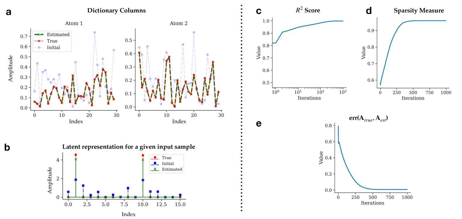
Figure 2: (a)Estimated dictionaries through the implicit generative map from the learned representations (differences in the estimated and true arise as the estimated atoms are not normalized). (b) Estimated latent representations (${\bm{Z}}$). (c) $R^{2}$ value of the predictions, 1-Sparsity measure of the latent representations (Appendix F), error in the similarity of the true and estimated dictionaries.

Discussion Figure 2 shows the results from the optimization process performed under Schedule 3 on the synthetic data which highlight a couple of observations. First, Figure 2 (a) shows the true, initial and final estimated generative maps from the learned representations with the true and final maps showing alignment. This is also captured in Figure 2(h). Similar alignment can be observed for the learned representations in Figure 2 (b) and (g) with the representations showing increasing level of sparsity (as defined in Appendix F) as shown in Figure 2(d). Second, we observe constraint satisfaction of the latent kernel structure happens early on in the optimization process as shown in Figure 2 (e) and the optimization dynamics thereafter closely follow the trajectory where the latent representations do not violate the constraint set. Finally, the correctness of the predictions made by using the learned representations and the estimated generative map is captured by the increasing trend in the $R^{2}$ value as shown in Figure 2 (f).

Comparison of different schedules: We also compare different schedules for the optimization process on the synthetic dataset. As alluded to in Section 5.1.1, the value of $\eta_{Z}$ under Schedule 3 is significantly smaller than the other proposed schedules. As a result, we expect Schedule 3 to converge at slower rate when compared the other schedules. This can be observed in Figure 3 which shows the comparison of the different schedules on the synthetic dataset as described in this section. We see that both Schedules 1 and 2 converge at a similar rate, which is faster than Schedule 3.

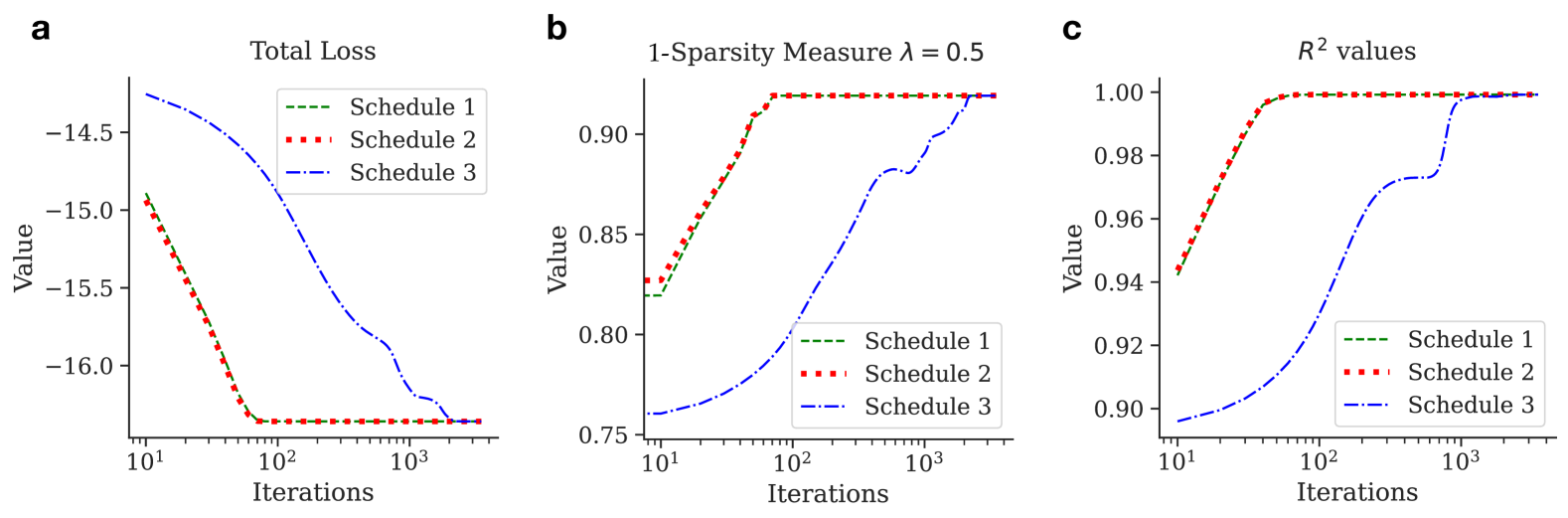
Figure 3: Comparison of the different optimization schedules on the synthetic dataset. The plot shows the convergence of the total loss, 1-sparsity measure (Appendix F) and $R^{2}$ values for the different schedules. We observe that Schedules 1 and 2 converge at a similar rate, which is faster than Schedule 3.

6.2 Applying KSM on real datasets with unknown latents

Setup and Initialization: We also applied the kernel matching framework to real datasets, namely, the MNIST dataset ($N=784,K=500$) (LeCun et al., 1998) and patches extracted from Natural Scenes dataset ($N=256,K=192$) (Olshausen and Field, 1996b) with significantly higher input dimension. We extract $\sim$ 9000 samples total from 5 different classes in the MNIST dataset and around 40000 random patches ($16\times 16$) extracted from a total of 10 images (each of size $512\times 512$) of the Natural Scenes dataset (Olshausen and Field, 1996a). Our approach involves using Schedule 1 of the optimization process on account of it showing faster rate of convergence in simulated experiments, as discussed in Section 5.1.1. We follow a similar initialization scheme for ${\bm{W}},{\bm{M}}_{i},{\bm{P}}_{i}$ and ${\bm{Z}}$ as discussed for the synthetic data experiments before. Table 1 contains the values of the hyperparameters used for the optimization process. The slower learning rate for ${\bm{W}}$ indicates that the loss surface in higher dimension tends to be more complex with multiple local minima, flat regions and saddle points and consequently require that gradient based methods proceed at a slower rate to avoid instabilities, thereby requiring more iterations of the optimization algorithm.

Figure 4 shows the dictionary or the generative maps learned from the representations on the MNIST and patches dataset. Each column of the dictionary represents a digit like structure for the MNIST dataset and gabor like structures for the patches extracted from Natural Scenes demonstrating selective receptive fields as discussed in (Olshausen and Field, 1996b). The sparsity of the learned representations progressively for both the datasets indicating increasing selectivity of the learned representations to the input data manifold.

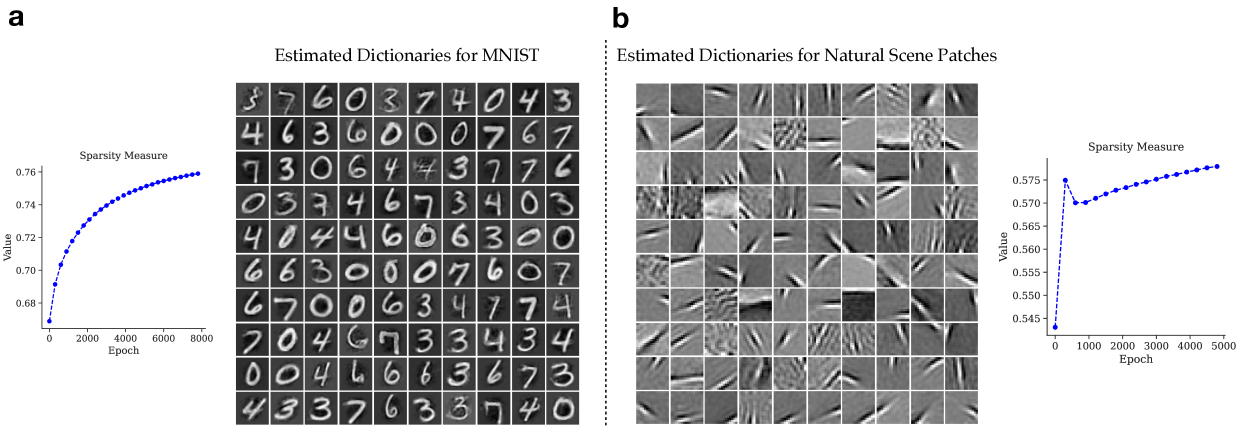
Figure 4: Estimated dictionaries using the implicit generative map on (a) the MNIST dataset (b) on patches extracted from natural scenes (100 atoms visualized) show that the learned representations implicitly learn generative maps that capture data features. The increasing sparsity measure also indicates that the learned representations progressively get sparser over the optimization process.

6.3 Synthetic data with Simplex Prior

We demonstrate the flexibility of the framework under different latent priors. We apply the objective in Proposition A.2 to the half moons dataset (Pedregosa et al., 2011) similar to approach undertaken in (Luther and Seung, 2022). by applying the objective in Proposition 1.2 to a synthetic moons dataset (Pedregosa et al., 2011). We sample $N=2500$ points from the dataset with an added Gaussian noise of 0.01 in magnitude, learning $K=12$ receptive fields serving as anchor points that are used to piece-wise approximate the manifold curvature. To initialize the optimization process outlined by Algorithm 2, we initialize ${\bm{W}}$ using random points on the input manifold. The initial latent representations were drawn from a standard normal distribution and projected on to the probability simplex. For the Lagrange multipliers, we initialize ${\bm{M}}_{i}=\frac{{\bm{W}}{\bm{W}}^{T}}{2}\,\forall\,i\in\{1,2,\dots,T\}$. The choice of hyperparameters in this experiment is also outlined in table 1. Note, in this case we do not have the parameter $\lambda$ and regularization is simply done by the parameter $\omega$.

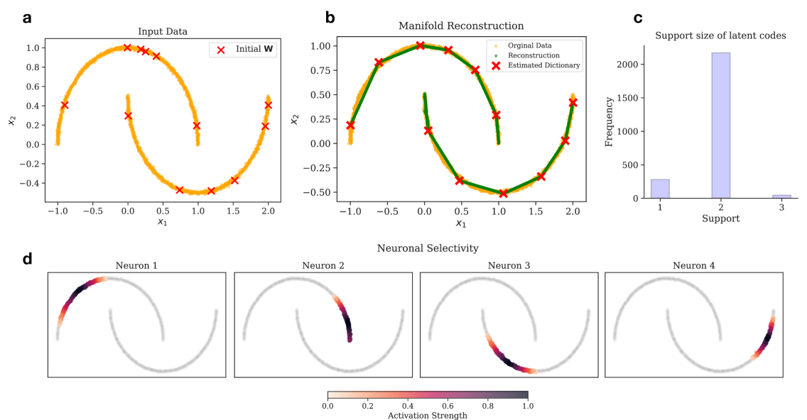
Figure 5: (a) An intrinsically one dimensional manifold represented by the two-moons dataset. (b) The piecewise approximated reconstruction by estimating the receptive fields through the implicit generative map learned from the representations. (c) $L_{0}$ norm of the latent codes indicating number of active neurons for each input sample. We see that most examples activate 2 neurons within a population indicating piece-wise linear reconstruction. This is directly tied to the intrinsic dimensionality of the input manifold which is one less than the modal $L_{0}$ norm. (d) Local selectivity of the neuronal population indicates that the neuronal activity is sensitive to local regions within the input manifold.

Discussion: Figure 5 shows the results of the optimization process on the synthetic moons dataset (Figure 5) (i). These estimated receptive fields, together with the learned representations, piece-wise linearize the input data manifold as shown in Figure 5(ii). From Figure 5(iii), we can note that a high percentage of the samples on the input manifold activate two neurons at a time in the population, since most of the learned representations have a support of size of 2, suggesting the input data manifold can be piecewise-linearized using one dimensional line segments. This can be used to estimate the intrinsic dimension of the manifold, which in the case of the moons dataset is one, thereby suggesting that the intrinsic dimension of the manifold is one less than the mode of the support of the latent representations. From Figure 5(iv), we observe four sample neurons out of $K=12$ that are activated by points on the input data manifold. The tuning curves of these neurons tile the manifold by having the maximum activations at the receptive fields indicated by the red crosses in Figure 5(ii), with the activation strength spreading along the geometry of the input data manifold. This suggests that metabolic constraints on neural activity tunes the learned representations to capture the geometric structure of the input data manifold.

Table 1: Choice of hyperparameters for the optimization process

Parameter	Sparse Dictionary
Learning			Manifold
Learning
	Synthetic	MNIST	Patches	Moons
$K$	16	500	192	12
$\lambda$	0.5	0.1	0.9	–
$\omega$	$10^{-4}$	$10^{-4}$	$10^{-4}$	0.1
$\rho$	1.0	1.0	1.0	1.0
$\eta_{W}$	0.01	$10^{-4}$	$10^{-4}$	$1.5\times 10^{-3}$
$T_{z}$	15	15	15	15
batch size $(B)$	128	128	128	128
max. epochs	3500	8000	5000	5500
$R^{2}$ value	1.0	0.78	0.86	0.98

7 Towards a biologically plausible implementation (SMPC architecture)

As mentioned before, kernel matching frameworks have been used to propose a biologically plausible model for learning representations (Pehlevan et al., 2018; Luther and Seung, 2022). These models learn representations by minimizing the distance between the input and latent kernel using feedforward and lateral connections which are learned using Hebbian and Anti-Hebbian rules. However, while good at learning representations representing the input, there is no explicit mechanism to learn generative maps in such frameworks. We conjecture that learning the kernel structure in the representation space could provide one way to extend kernel matching approaches to learn generative maps, which traditionally require top-down interactions i.e. feedback from higher cortical layers to lower ones. This idea of top-down interactions between different cortical layers forms the basis of predicting coding approaches which have been used to provide a mathematical framework for visual processing in the brain (Rao and Ballard, 1999; Keller and Mrsic-Flogel, 2018; Boutin et al., 2020, 2021). Using the objective developed in Proposition A.1, we discuss a biologically plausible extension to the classical kernel matching framework in (Pehlevan et al., 2018; Luther and Seung, 2022) incorporating top-down interactions for learning generative maps alongside representations.

We start with articulating a relaxed version of the objective in Equation 7 given as follows:

$$\underset{{\bm{Y}},{\bm{Z}},{\bm{\Omega}}}{\min}\,\, -\frac{1}{2T^{2}}\operatorname{Tr}({\bm{X}}^{T}{\bm{X}}{\bm{Y}}^{T}{\bm{Y}})+\frac{\lambda}{T}\|{\bm{Z}}\|_{1,1}+\frac{\rho}{T}\|{\bm{Y}}-{\bm{\Omega}}{\bm{Z}}\|_{F}^{2}$$ (15)

We introduce a standard kernel using an intermediate representation ${\bm{Y}}$ in the trace term in Equation 15, replacing the structured latent kernel in Equation 7. This intermediate representation is related to the final latents ${\bm{Z}}$ through a linear transformation ${\bm{\Omega}}$, which is enforced by the penalty term $\frac{\rho}{2T}\|{\bm{Y}}-{\bm{\Omega}}{\bm{Z}}\|_{F}^{2}$ in the objective, where $\rho$ controls the strength of the penalty. Under low penalty values, i.e, when ${\bm{Y}}\approx{\bm{\Omega}}{\bm{Z}}$, the trace term in the objective reduces to computing a similarity measure between the standard kernel of the input matrix ${\bm{X}}$ and the structured kernel of the representations ${\bm{Z}}$, with the structure determined by the matrix ${\bm{\Omega}}^{T}{\bm{\Omega}}$. Unlike the formulation in Equation 7, we relax the constraints on the kernel structure ${\bm{\Omega}}$ for the formulation above, allowing it to be governed by the data itself. Accordingly, as outlined in §3, the implicit generative map can be articulated as $\hat{\bm{A}}=\dfrac{{\bm{X}}{\bm{Z}}^{T}({\bm{\Omega}}^{T}{\bm{\Omega}})}{T}$, where ${\bm{\Omega}}^{T}{\bm{\Omega}}$ determines the kernel structure in the latent space, similar to ${\bm{H}}^{-1}$.

Connection to classical MDS and stabilizing the learning dynamics: We augment the objective in Equation 15 by adding a penalty term comprising of the Frobenius norm of the kernel of ${\bm{Y}}$, resulting in the update objective as follows:

$$\underset{{\bm{Y}},{\bm{Z}},{\bm{\Omega}}}{\min} -\frac{1}{2T^{2}}\operatorname{Tr}({\bm{X}}^{T}{\bm{X}}{\bm{Y}}^{T}{\bm{Y}})+\frac{\alpha}{4T^{2}}\operatorname{Tr}({\bm{Y}}^{T}{\bm{Y}}{\bm{Y}}^{T}{\bm{Y}})+\frac{\lambda}{T}\|{\bm{Z}}\|_{1,1}+\frac{\rho}{T}\|{\bm{Y}}-{\bm{\Omega}}{\bm{Z}}\|_{F}^{2}$$ (16)

$$\Longleftrightarrow\underset{{{\bm{Y}},{\bm{Z}},{\bm{\Omega}}}}{\min} \,\,\frac{1}{4T^{2}}\|{\bm{X}}^{T}{\bm{X}}-{\bm{Y}}^{T}{\bm{Y}}\|_{F}^{2}+\frac{\lambda}{T}\|{\bm{Z}}\|_{1,1}+\frac{\rho}{T}\|{\bm{Y}}-{\bm{\Omega}}{\bm{Z}}\|_{F}^{2}$$

where, the lower objective is obtained by completing the squares. For our case we choose $\alpha=1$. The addition of the term $\frac{1}{4T^{2}}\operatorname{Tr}({\bm{Y}}^{T}{\bm{Y}}{\bm{Y}}^{T}{\bm{Y}})$ to the objective in equation 16 introduces a penalty on the norm of the intermediate kernel which is absent in Equation 15. This additon transforms the objective in Equation 16 into an upper bound on the objective in Equation 15. The kernel norm penalty enforces a stronger similarity between the input and the intermediate representations by aligning the norm of the respective kernels. Furthermore, this converts the trace term in Equation 15 into a Classical Multidimensional Scaling (MDS) objective (Borg and Groenen, 2007). A key benefit of this augmentation is the stabilization of the learning dynamics during optimization with respect to the intermediate representation ${\bm{Y}}$. The original formulation in Equation 15 can result in runaway dynamics in certain directions of the optimization space, due to the strong concavity introduced by the negative of the trace term with respect to ${\bm{Y}}$. Incorporating the kernel norm penalty address this issue by bounding the objective in Equation 16 from below. Consequently, the entire objective now comprises of two parts – a similarity matching term between the input ${\bm{X}}$ and the intermediate representations ${\bm{Y}}$ and prediction error term between the intermediate and the final representations ${\bm{Y}}$ and ${\bm{Z}}$ respectively. Employing Legendre transformation on the objective in Equation 16 allows us to derive an online version of the objective similar to the ones as discussed in §2. We articulate the online objective in the proposition below:

Proposition 1.4.

Let $R_{2}$ be the optimization problem as described below. Then $R_{2}$ is equivalent to Equation 16.

$$R_{3}:\underset{{\bm{Y}},{\bm{Z}},{\bm{\Omega}},{\bm{W}}}{\min}\,\underset{{\bm{M}}}{\max} \,\frac{1}{T}\sum\limits_{i=1}^{T}\left(-{\bm{x}}_{i}^{T}{\bm{W}}^{T}{\bm{y}}_{i}+\frac{1}{2}\operatorname{Tr}({\bm{W}}^{T}{\bm{W}})+\frac{1}{2}{\bm{y}}_{i}^{T}{\bm{M}}{\bm{y}}_{i}-\frac{1}{4}\operatorname{Tr}({\bm{M}}^{T}{\bm{M}})+\lambda\|{\bm{z}}_{i}\|_{1}+\frac{\rho}{2}\|{\bm{y}}_{i}-{\bm{\Omega}}{\bm{z}}_{i}\|^{2}\right)$$ (17)

We note that the objective described in Equation 17 is a min max optimization problem. We exchange the order of optimization with respect to optimization variables ${\bm{M}}$ and the latent representations ${\bm{Z}}$ and ${\bm{Y}}$. The first exchange between ${\bm{M}}$ and ${\bm{Z}}$ is possible on the account of the objective being decoupled with respect to these variables. The second exchange between ${\bm{M}}$ and ${\bm{Y}}$ can be done as the objective satisfies the saddle point property (proof in Appendix, similar to (Pehlevan et al., 2018)). The resultant optimization problem can be written as:

Proposition 1.5.

Let $R_{4}$ be the optimization problem as described below. Then $R_{4}$ is equivalent to Equation 17.

$$R_{4}:\underset{{\bm{\Omega}},{\bm{W}}}{\min}\,\underset{{\bm{M}}}{\max}\,\underset{{\bm{Z}},{\bm{Y}}}{\min} \,\frac{1}{T}\sum\limits_{i=1}^{T}\left(-{\bm{x}}_{i}^{T}{\bm{W}}^{T}{\bm{y}}_{i}+\frac{1}{2}\operatorname{Tr}({\bm{W}}^{T}{\bm{W}})+\frac{1}{2}{\bm{y}}_{i}^{T}{\bm{M}}{\bm{y}}_{i}-\frac{1}{4}\operatorname{Tr}({\bm{M}}^{T}{\bm{M}})+\lambda\|{\bm{z}}_{i}\|_{1}+\frac{\rho}{2}\|{\bm{y}}_{i}-{\bm{\Omega}}{\bm{z}}_{i}\|^{2}\right)$$ (18)

We can now optimize the objective in Equation 18 by applying stochastic gradient descent-ascent algorithm, first optimizing with respect to the representations ${\bm{Y}}$ and ${\bm{Z}}$ followed by updating the sample independent parameters ${\bm{W}},{\bm{M}},{\bm{\Omega}}$. We articulate the gradient dynamics of the optimization process in Appendix E and use the dynamics of each of the variables to derive a predictive coding network as discussed in (Bogacz, 2017), where the synaptic weights are learned using Hebbian and anti-Hebbian rules. Here ${\bm{Y}}$ and ${\bm{Z}}$ model neuron activations, with ${\bm{Z}}$ being modeled as a two cell neuron, whereas, the sample independent terms ${\bm{W}},{\bm{M}}$ and ${\bm{\Omega}}$ model the synapses.

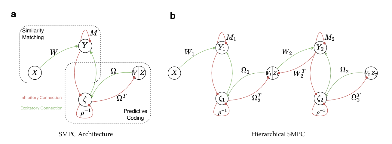
Figure 6: (a) The SMPC architecture for kernel similarity matching. The bottom-up interactions in encoding ${\bm{Y}}$ from the input ${\bm{X}}$ and the top-down interactions in predicting ${\bm{Y}}$ from the latent activity ${\bm{Z}}$ are modulated through the interneuron $\bm{\zeta}$. The inhibitory connections and the excitatory connections are obtained from the gradient dynamics of the optimization process (Appendix E) (b) Hierarchical extension of the SMPC architecture, where the learned latents in the first layer act as an input in the second layer. Unlike classical feed-forward models for representation learning, there is an feedback loop from the higher layer to the lower layer. In our implementation, the neuronal population denoted by ${\bm{Y}}$ acts as an inhibitory neuron and the population denoted by ${\bm{V}}|{\bm{Z}}$ acts as an excitatory neuron in accordance with Dale’s law, however, the interneuron sends out mixed signals propagating the excitation from the higher layers and inhibition from the lower layers. The interneuron population could be split to make the architecture satisfy Dale’s law, however, we omit that here for simplicity.

Modeling the prediction error using interneurons: The prediction error between the final latent representation ${\bm{Z}}$ and the intermediate representation ${\bm{Y}}$ is modeled using interneurons denoted by $\bm{\zeta}$. Interneurons have been used in earlier work to describe how neurons mediate recurrent communication to perform operations such as statistical whitening (Lipshutz et al., 2022). These interneurons often called error neurons in predictive coding literature, are used to minimize prediction errors in line with redundancy reduction hypothesis of neural coding, allowing the brain to focus on unexpected stimuli to improve the accuracy of predictions (Simoncelli and Olshausen, 2001; Friston, 2005). In our case, these interneurons mediate between bottom-up interactions stemming from encoding ${\bm{Y}}$ through kernel similarity matching with the input ${\bm{X}}$ and the top-down interactions in predicting ${\bm{Y}}$ from the latent representations ${\bm{Z}}$. As a result, we call the architecture denoted in Figure 6(a) as the SMPC (similarity matching predictive coding) architecture, where the learning dynamics of the synapses follow local plasticity rules. Furthermore, the structure of the SMPC architecture can be extended to form a hierarchical network which can be used to model information flow between different cortical layers (Figure 6 (b)). We keep the discussion to a single layer network and leave the extension to a hierarchical network as future work.

7.1 Numerical Experiments

We now investigate the ability of the SMPC architecture to implicitly learn generative maps on simulated datasets in the section below. We begin with sparsity constraints on the latent space.

Setup: We applied the SMPC architecture (Figure 6(a)) to simple 2D dataset in Figure 7(a). The dataset consists of $N=512$ points generated by atoms of dictionary ${\bm{A}}\in{\mathbb{R}}^{2\times 2}$, where the atoms are chosen along two directions such that correlation between the atoms is $0.14$. This low mutual coherence between the atoms is necessary for sparse dictionary learning (Donoho, 2006). The latent representations ${\bm{Z}}$ are generated along the $x$ and $y$ axis as shown in Figure 7(a). Additionally, a small amount of additive Gaussian noise (standard deviation = 0.01) was added to the samples.

To speed up the optimization process, the synaptic updates were performed using batches sampled from the data. For this 2d dataset, the batch size was set to be equal to the length of the dataset. The learning rates for the neuronal dynamics $\eta_{\bm{Y}},\eta_{\bm{Z}}$ were set to $0.1$ and run for $10$ iterations each, with $\eta_{\bm{W}}=0.05\ll\eta_{\bm{M}}=0.1$ as suggested in (Luther and Seung, 2022) and are run for $5$ iterations to indicate the slower learning cycle of the synaptic weights. Our implementation assumes that interneurons $\zeta$ are highly sensitive with the highest learning rates, implying that their dynamics remain at fixed points throughout the optimization process. The values of $\rho$ and $\lambda$ were set to $5.$ and $0.8$ respectively. The initialization details for the optimization process are provided in the appendix. The results of the simulation are shown in Figure 7.

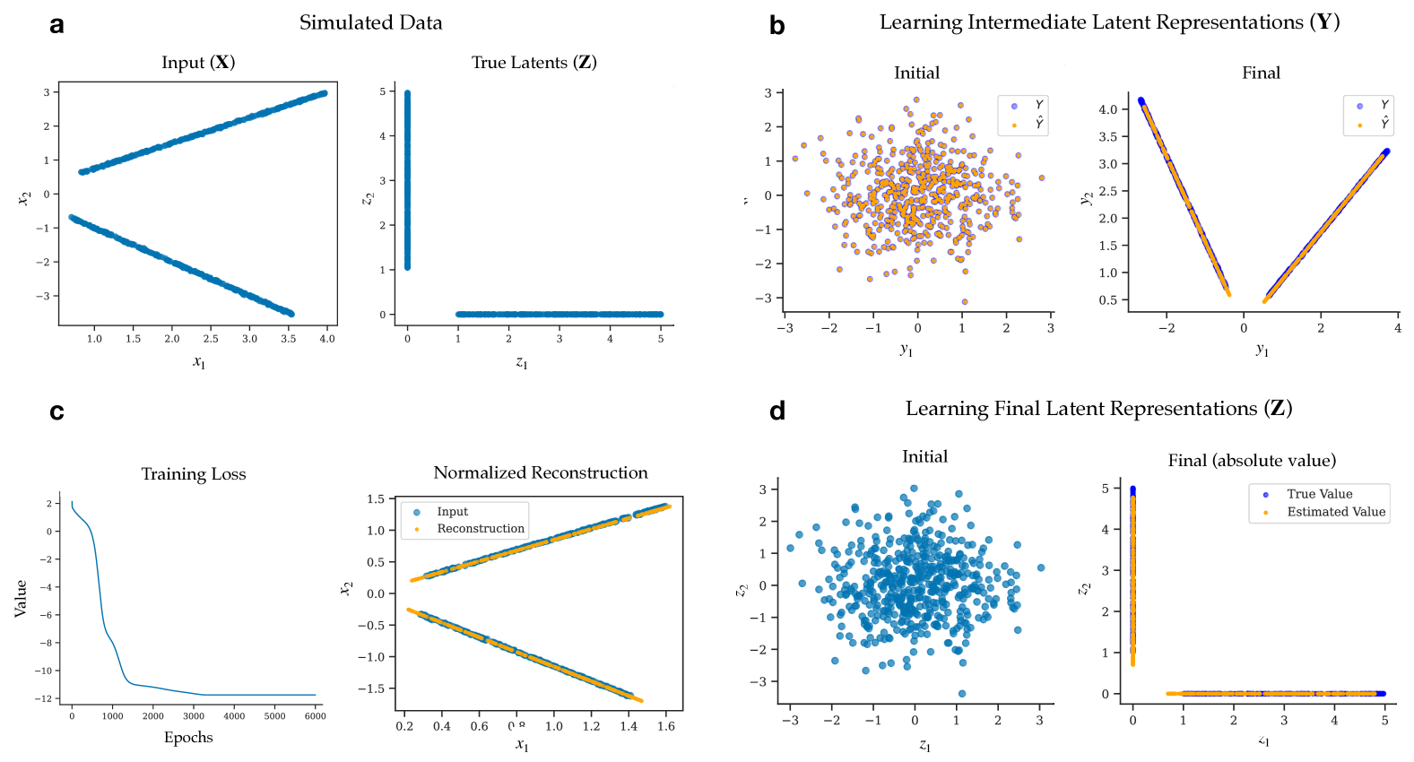
Figure 7: Results of applying the SMPC architecture on a 2D dataset. (a) Simulated 2D dataset with true latent representations ${\bm{Z}}$. (b) Intermediate representations (${\bm{Y}}$) governed by bottom-up interactions from the input ${\bm{X}}$ and their predictions from top-down interactions ($\hat{\bm{Y}}={\bm{\Omega}}{\bm{Z}}$). The interneuron $\bm{\zeta}$ effectively modulates the communication between the intermediate and final latents. (c) Decrease in the overall objective value as the optimization proceeds along with the predicted derived from the implicit generative map using the learned representations ${\bm{Z}}$ (shown in (d)) and the synaptic weights ${\bm{\Omega}}$. We show normalized input and prediction, normalized by data variance, to make sure any scaling effects in reconstruction are minimized. (d) The final representations ${\bm{Z}}$ learned by the SMPC architecture with the initial values prior to the optimization showed on the left.

Discussion: Our results indicate that the model successfully recovers both the latent structure and its corresponding value s(Figure 7(d)). The interneuron facilitates bottom-up and top-down communication between the intermediate and the final latents given by ${\bm{Y}}$ and ${\bm{Z}}$ respectively. This is evident in Figure 7 (b) where the intermediate latent ${\bm{Y}}$ aligns well with its corresponding top-down prediction, $\hat{\bm{Y}}={\bm{\Omega}}{\bm{Z}}$. To compute the predicted input, we use $\hat{\bm{A}}=\frac{{\bm{X}}{\bm{Z}}^{T}({\bm{\Omega}}^{T}{\bm{\Omega}})}{T}$ to compute the generative map, as discussed in the previous section and articulated in §3, with the prediction being given as $\hat{\bm{X}}=\frac{{\bm{X}}{\mathcal{K}}_{\bm{Z}}}{T},\,{\mathcal{K}}_{\bm{Z}}=({\bm{\Omega}}{\bm{Z}})^{T}({\bm{\Omega}}{\bm{Z}})$. Here ${\bm{Z}}$ and ${\bm{\Omega}}$ were estimated from the optimization process. While $\hat{\bm{X}}$ as calculated before, captures the structure of the input data ${\bm{X}}$, in our experiments, we found that the predicted input $\hat{\bm{X}}$ aligns with the input data ${\bm{X}}$ when the data is variance normalized, i.e. ${\bm{x}}_{i}\leftarrow\dfrac{{\bm{x}}_{i}}{\sqrt{\frac{1}{T}\sum\limits_{j=1}^{T}\|{\bm{x}}_{j}\|^{2}_{2}}}$. This is demonstrated in Figure 7(c). A reason for this could be the fact that we are matching kernels instead of explicit reconstruction, suggesting that while correlation structure is preserved, the actual data norm may not be.

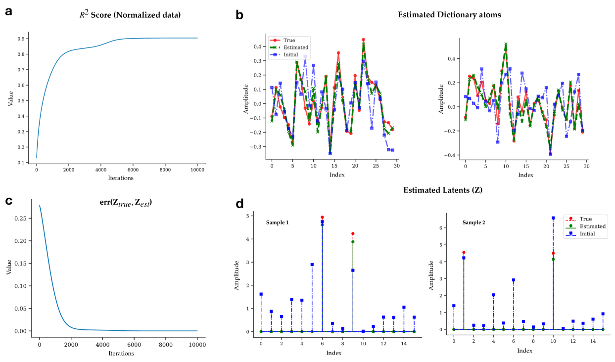
Figure 8: Applying the SMPC architecture on a higher dimensional dataset ($N=30$). (a) $R^{2}$ score plotted for normalized input (${\bm{X}}$) and predicted input $(\hat{\bm{X}}$). (b) The implicit generative maps computed using learned representations (${\bm{Z}}$) (shown in (d)) and the synaptic weights ${\bm{\Omega}}$. (c) Sine similarity error between the true and estimated latents (${\bm{Z}}$) with (d) showing two sample latents – the true value, the initial value before optimization and the final value after optimization. The estimated latents align with the true latents, however, we see the lack of constraints on the kernel structure affects the $R^{2}$ value ( < 1) which reduces when the mutual coherence in the dictionary columns increase.

Scaling up the data dimension: Next, we scaled up the data dimensions to $N=30$ (similar to §6.1) to understand the behavior of the SMPC architecture on higher dimensional dataset. We generate the data using a similar process as before (§6.1), except the dictionary ${\bm{A}}$ was subjected to an additional Gram-Schmidt orthogonalization to ensure that the mutual coherence between the atoms was low. The amplitude latent values, ${\bm{Z}}$ were sampled independently from a ${\mathcal{N}}(5,1)$ distribution, with $87.5\%$ of the positions along a given dimension for every latent set to zero to ensure sparse representations. This process is similar to the generated latents shown in Figure 7(a). The initialization details for the implementation are discussed in the appendix. The results of the optimization process are shown in Figure 8. Figure 8(a) shows the $R^{2}$ value computed for the normalized input and the normalized predictions from the implicit generative maps, computed as before, and the estimated latents (${\bm{Z}}$). We see that the model is able provide good predictions (reflected by the $R^{2}$ value of 0.9). Figure 8(b) shows the estimates of the implicit generative maps ($\hat{\bm{A}}$). Figure 8(c) shows the sine similarity between the estimated latents and the true values which is computed as $\displaystyle\text{err}({\bm{Z}}_{true},{\bm{Z}}_{est})=\dfrac{1}{T}\sum\limits_{i=1}^{T}\left[1-\left(\dfrac{\langle{\bm{z}}_{i}^{(t)},{\bm{z}}_{i}^{(e)}\rangle}{\|{\bm{z}}_{i}^{(t)}\|\|{\bm{z}}_{i}^{(e)}\|}\right)^{2}\right]$, where ${\bm{z}}_{i}^{(t)}$ are the true latent values and ${\bm{z}}_{i}^{(e)}$ are the estimated latent representations. The error metric goes to zero as the estimated latents align with the true latents as shown in Figure 8(c). Figure 8(d) shows the true values, initial values prior to optimization and the estimated values post optimization. We observe that the estimated latents align with the true latents, however, the relaxed nature of the optimization problem affects the $R^{2}$ value which is less than 1, which suggests that imposing the constraints on the latent kernel structure plays a role in improving the implicit generative maps. Finally, varying $\alpha$ in Equation 16, we found that $\alpha=1$ produced the best $R^{2}$ value.

Imposing metabolic constraints capture the curvature of the data manifold, but proper prediction warrants appropriate kernel structure: Finally, we apply metabolic constraints on the latent activity, imposed in the form a probability simplex, to understand how the representations capture information about the input geometry in the SMPC architecture (similar to §6.3). The initialization details for the optimization process are discussed in the appendix, with Figure 9 demonstrating the results at the end of the optimization process. Figure 9 (a) demonstrates the input data manifold (we use the moons dataset (Pedregosa et al., 2011) similar to §6.3), alongside the predicted values at the beginning of the optimization process and the final predicted values. Additionally, we plot the implicit generative maps, estimated using the circuit parameters (red cross). We see that the predicted inputs are able to capture the curvature of the input manifold and correlates well (good similarity measure) with the input data, with the implicit generative maps following the curvature of the individual manifolds to form. However, the prediction does not align perfectly with the input due to the relaxed nature of the optimization problem, which lacks any constraints on the kernel structure of the latent space. Nevertheless, we see emergence of local receptive field properties of individual neurons (shown in Figure 9 (b)) similar to the ones observed in §6.3, suggesting that the simplex constraints tune neurons to capture the geometry of the input manifolds.

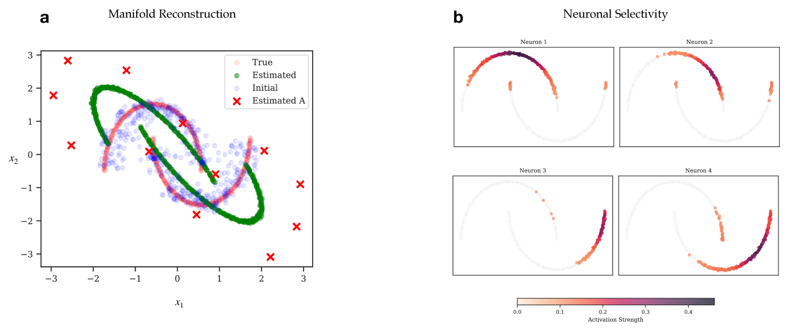
Figure 9: Applying probability simplex constraints on the latent representations. (a) Predicted inputs (green) ($\hat{\bm{X}}$) from the two moons dataset alongside the true values (red) and the initial value (blue) prior to the optimization process. We see that the predicted inputs is able to capture the shape and structure of the data manifold (due to similarity alignment), however, due to the relaxed nature of the optimization problem, the prediction does not align perfectly with the input. The estimated receptive fields (indicated by a red cross), also circumvents the predicted manifold along its curvature. The final $R^{2}$ value achieved was 0.7. (b) Neuronal selectivity, shows the input samples that the a particular neuron is getting activated for, demonstrating local receptive nature of the neurons, albeit wider than the case in Figure 5.

In the sets experiment above, we observe, that the SMPC architecture is able to learn the underlying latent representations in a neurally plausible manner by incorporating bottom up and top-down interactions. Furthermore, the circuit parameters are able to capture features needed to construct a generative map as shown by an $R^{2}$ value which is greater than $0.5$. Nonetheless, the implicit generative maps thus estimated differ from the true values, due to the relaxed nature of the optimization problem that does not impose any constraints on the structure of the kernel in the latent space. The imposition of constraints on the kernel structure (governed by ${\bm{\Omega}}$) while maintaining local plasticity rules for synaptic learning will be investigated in a future work.

8 Conclusion

We introduce a kernel similarity matching framework for learning representations within a generative context. We explore this method in the realm of dictionary learning and show that learning the kernel function in the latent space alongside the representations can facilitate learning of generative maps between the representation and the input space respectively. Our approach formulates this hypothesis as a constrained optimization problem with the constraints applied on the latent kernel structure, extending prior works by (Pehlevan et al., 2018; Luther and Seung, 2022). To address the computational challenges inherent in the optimization of the objective, we developed a separable formulation that distributes the objective and the constraints across individual samples, thereby enabling online optimization. Finally, we develop an ADMM based algorithm to formulate the gradient dynamics of the optimization variables, and draw connections to standard optimization algorithms deployed used in similar settings (5.1.1)

The versatility of our framework is further illustrated, when we adapt it to learn a generative framework for manifold learning. Here, we reconstruct the input manifold piece-wise by learning receptive fields along its curvature. This is achieved by imposing a probability simplex constraint on the latent representations, which is inspired by metabolic limits on neuronal firing. The representations implicitly capture the geometry of the input manifold by learning receptive fields along the data manifold which in conjunction with the learned latent representations, piece-wise approximates the input data manifold. This is in stark contrast with geometry preserving feature learning techniques such as t-SNE or Isomap, where the learned representations do not capture an implicit generative map. Furthermore, in our case, the number of active neurons within the population of latent representations estimate the intrinsic dimension of the input manifold, which can lead to a normative way of understanding how geometric structure of the input data manifold play a role in shaping what the population encodes.

Building on these results, we extend our kernel similarity objective to design a predictive coding network based on the gradient dynamics of the associated variables. The proposed architecture facilitates representation learning by integrating bottom-up interactions through similarity matching and top-down interactions via predictive coding, with an inter-neuron system regulating these interactions. We applied this framework to simulated datasets and showed that the network can estimate the latent representations with reasonable reconstruction of the input data. However, in the absence of structural constraints on the representation kernel, the generated input predictions—though similar in structure to the true input—deviate from the actual underlying values. Addressing this limitation in future work may involve imposing explicit constraints on the latent kernel structure while preserving local plasticity to ensure biological plausibility. Another challenge the architecture faces, as depicted in Figure 6(a) is the weight transport problem, where weight of one synapse (${\bm{\Omega}}$) needs to be copied to a different synapse (${\bm{\Omega}}^{T}$). Recent work by (Millidge et al., 2020) provides possible approaches in dealing with this problem. Other recent arguments on neural plausibility explore three-factor Hebbian rules for learning which (Pogodin and Latham, 2020) use to learn representations in a kernelized setting by regulating the mutual information between the input and the latent representations, known as the information bottleneck principle (Tishby et al., 2000).

While we have focused on two specific kernel matching scenarios for representation learning, our framework’s inherent flexibility invites exploration of alternative kernel functions and the unique generative behaviors they induce. Moreover, although our proposed architecture offers a mechanistic model for synaptic plasticity, its hierarchical extensions (Figure 6(b)) and implementation in physiological settings remain promising directions for future research.

9 Acknowledgements

We thank Dr. Abiy Tassisa, Department of Mathematics, Tufts University, Prof. Venkatesh Murthy, Harvard University, and members of the Ba lab for their valuable feedback and discussions. SC was partially supported by the Kempner Graduate Fellowship and both SC and DB were partially supported by the National Science Foundation (grant DMS-2134157). The computations in this paper were performed on the Faculty of Arts and Sciences Research Computing (FASRC) cluster at Harvard University, and was supported in part by the Kempner Institute for the Study of Natural and Artifical Intelligence at Harvard University. This research was carried out in part thanks to funding from the Canada First Research Excellence Fund, awarded to PM through the Healthy Brains, Healthy Lives initiative at McGill University.

Appendix A Proof of Lemma 1

Proof.

Let us assume without loss of generality, $\underset{{\bm{x}}}{\min}\,\underset{{\bm{y}}}{\min}\,\,f({\bm{x}},{\bm{y}})>\underset{{\bm{y}}}{\min}\,\underset{{\bm{x}}}{\min}\,\,f({\bm{x}},{\bm{y}})$.
Let $f({\bm{x}}^{*},{\bm{y}}^{*})=\underset{{\bm{x}}}{\min}\,\underset{{\bm{y}}}{\min}\,\,f({\bm{x}},{\bm{y}})$ and $({\bm{x}}^{\dagger},{\bm{y}}^{\dagger})=\underset{{\bm{y}}}{\min}\,\underset{{\bm{x}}}{\min}\,\,f({\bm{x}},{\bm{y}})$
then, we have $f({\bm{x}}^{*},{\bm{y}}^{*})>f({\bm{x}}^{\dagger},{\bm{y}}^{\dagger})$. However,

$$f({\bm{x}}^{\dagger},{\bm{y}}^{\dagger}) \geq\underset{{\bm{x}}}{\min}\,\,f({\bm{x}},{\bm{y}}^{\dagger})$$

$$\geq\underset{{\bm{x}}}{\min}\,\underset{{\bm{y}}}{\min}\,\,f({\bm{x}},{\bm{y}})$$

$$=f({\bm{x}}^{*},{\bm{y}}^{*})\implies\text{A contradiction}$$

Therefore, the only possibility is $f({\bm{x}}^{*},{\bm{y}}^{*})=f({\bm{x}}^{\dagger},{\bm{y}}^{\dagger})$ or $\underset{{\bm{x}}}{\min}\,\underset{{\bm{y}}}{\min}\,\,f({\bm{x}},{\bm{y}})=\underset{{\bm{y}}}{\min}\,\underset{{\bm{x}}}{\min}\,\,f({\bm{x}},{\bm{y}})$ ∎

A.1 Proof of proposition 1.1

Proof.

Starting from $P_{1}$, using lemma 1, we can rewrite $P_{1}$ as:

$$\underset{{\bm{Z}},{\bm{A}}}{\min}\,\,\frac{1}{2T}\|{\bm{X}}-{\bm{A}}{\bm{Z}}\|^{2}_{F}+\frac{\lambda}{T}\|{\bm{Z}}\|_{1}+\frac{\omega}{2}\|{\bm{A}}\|_{F}^{2}\qquad\omega>0$$

where, we have changed the order of minimization. The inner optimization is now a strongly convex problem with respect to the dictionary ${\bm{A}}$ and has a unique optimum at ${\bm{A}}^{*}=\dfrac{{\bm{X}}{\bm{Z}}}{T}\left(\dfrac{{\bm{Z}}{\bm{Z}}^{T}}{T}+\omega I\right)^{-1}$. Plugging it back into the objective and defining ${\bm{H}}=\dfrac{{\bm{Z}}{\bm{Z}}^{T}}{T}+\omega I$, we end up with the objective in $Q_{1}$. ∎

A.2 Proof of proposition 1.2

Proof.

Similar to before we switch the order of optimization in $P_{2}$ using lemma 1 to obtain:

$$\underset{{\bm{Z}},{\bm{A}}}{\min}\,\,\frac{1}{2T}\|{\bm{X}}-{\bm{A}}{\bm{Z}}\|^{2}_{F}+\frac{\omega}{T}\sum\limits_{k=1}^{K}\sum\limits_{l=1}^{T}z_{kl}\|{\bm{x}}_{l}-{\bm{a}}_{k}\|_{2}^{2}\qquad\omega>0$$

Solving the inner optimization w.r.t. ${\bm{A}}$ we end up with ${\bm{A}}^{*}=(1+\omega)\dfrac{{\bm{X}}{\bm{Z}}^{T}{\bm{H}}^{-1}}{T}$, where ${\bm{H}}=\dfrac{{\bm{Z}}{\bm{Z}}^{T}}{T}+\omega{\bm{D}},\,\,\text{and}\,\,{\bm{D}}=\text{Diag}\left(\dfrac{{\bm{Z}}\mathbf{1}_{T}}{T}\right)$, is a diagonal matrix. Substituting in back in $P_{2}$ we get

$$\underset{{\bm{Z}},{\bm{H}}}{\min} -\frac{(1+\omega)^{2}}{2T^{2}}\operatorname{Tr}({\bm{X}}^{T}{\bm{X}}{\bm{Z}}^{T}{\bm{H}}^{-1}{\bm{Z}})$$ (19)

s.t. $$\,\,{\bm{Z}}^{T}\mathbf{1}_{K}=\mathbf{1}_{T}$$

$$\,\,{\bm{Z}}\geq 0$$

$$\,\,{\bm{H}}=\frac{{\bm{Z}}{\bm{Z}}^{T}}{T}+\omega{\bm{D}}$$

Scaling the objective in equation 19 by $1/(1+\omega)^{2}$ we get the objective in $Q_{2}$. ∎

Appendix B Projection onto the probability simplex induces subtractive normalization

In this section we show that how the projection onto the probability simplex induces a normalization effect on the overall population activity. We consider the following optimization problem depicting the output of the simplex projection:

$${\bm{z}}=\arg\underset{x\in{\mathbb{R}}^{D}}{\min} \frac{1}{2}\|{\bm{x}}-{\bm{y}}\|^{2}$$ (20)

s.t. $$\,\,{\bm{x}}^{T}\mathbf{1}=1$$

$$\,\,{\bm{x}}\geq 0$$

where, ${\bm{z}}$ denotes the population activity and ${\bm{y}}$ denotes the input to the population. Without loss of generality, we assume the input activity to be sorted such that $y_{1}\geq y_{2}\geq\dots y_{D}$. The solution of the above optimization problem is given by:

$$z_{i}=\max\left(0,y_{i}-\lambda({\bm{y}})\right)$$ (21)

with $\lambda({\bm{y}})=\dfrac{1}{\rho}\left(\sum\limits_{i=1}^{\rho}y_{i}-1\right)$, where $\rho=\max\{1\leq i\leq D:y_{i}-\dfrac{1}{\rho}\left(\sum\limits_{i=1}^{\rho}y_{i}-1\right)>0\}$. The threshold $\lambda({\bm{y}})$ is adaptive and is derived by computing a running mean of the population activity sorted in decreasing order (if the activity is not sorted, then we sort the activity first and then compute the sum). We refer the reader to Wang and Carreira-Perpinán [2013] for a detailed proof of the above result.

We see from Equation 21 that the output of the simplex projection involves a thresholding operation on the input activity with an adaptive threshold computed by calculating a sort of running mean over the population activity which is then subtracted from the input. We call this operation subtractive normalization, as the result of this operation is that the output activity is normalized to sum to unity.

Appendix C ADMM dynamics for solving the KSM problem

In this section we layout the gradient dynamics for each step of the ADMM optimization articulated in Algorithm 2 for the separable Lagrangian of the kernel similarity matching problem with sparsity constraints on the latent space.

C.1 Dynamics with Sparsity constraints on the latent space

Given objective:

$$\underset{{\bm{W}},{\bm{z}}_{i},{\bm{P}}_{i}}{\min} \,\,-\frac{1}{T}\sum\limits_{i=1}^{T}\left({\bm{x}}_{i}^{T}{\bm{W}}^{T}{\bm{z}}_{i}\right)+\frac{1}{2T}\sum\limits_{i=1}^{T}\operatorname{Tr}\left({\bm{W}}^{T}{\bm{P}}_{i}{\bm{W}}\right)+\frac{\lambda}{T}\sum\limits_{i=1}^{T}\|{\bm{z}}_{i}\|_{1}$$ (22)

s.t. $$\,\,{\bm{P}}_{i}={\bm{z}}_{i}{\bm{z}}_{i}^{T}+\omega\mathbf{I}\qquad\forall\,\,i\in\{1,2,\dots,T\}$$

The above objective involves optimizing over ${\bm{W}},{\bm{z}}_{i},{\bm{P}}_{i}$. For a given iteration $k$ of the ADMM algorithm (Algorithm 2), the update dynamics of each of the optimization subproblem in each step of the ADMM algorithm is given below, where $\tau$ represents the current iteration in the optimization subproblem.

• Z-Step
  

  The Z-Step for the $(k+1)^{th}$ epoch involves the following optimization:

  $${\bm{z}}_{i}^{k+1}\leftarrow\underset{{\bm{z}}}{\arg\min}\,\,\mathcal{L}_{i}({\bm{z}}_{i},{\bm{P}}_{i}^{k},{\bm{M}}_{i}^{k})$$

  where,

  $$\mathcal{L}_{i}=-{\bm{x}}_{i}^{T}{\bm{W}}{\bm{z}}_{i}+\frac{1}{2}\operatorname{Tr}({\bm{W}}^{T}{\bm{P}}_{i}{\bm{W}})+\lambda\|{\bm{z}}_{i}\|_{1}+\rho\left\|{\bm{z}}_{i}{\bm{z}}_{i}^{T}+\omega{\bm{I}}-{\bm{P}}_{i}+\frac{{\bm{M}}_{i}}{\rho}\right\|_{F}^{2}$$

  The Lagrangian described before is a quartic function in ${\bm{z}}_{i}$ involving smooth and non-smooth functions, so we resort to gradient based methods to optimize for ${\bm{z}}_{i}$. Specifically, we use proximal gradient descent methods to account for the $\ell_{1}$ norm regularization. The update dynamics for the $\tau+1^{th}$ iteration of the proximal method is given as:

  $${\bm{z}}_{i}^{(\tau+1),k} ={\mathcal{S}}_{\frac{\lambda}{\eta}}\left[{\bm{z}}_{i}^{(\tau),k}-\eta_{Z}\left\{-{\bm{W}}^{k}{\bm{x}}_{i}+2\rho\left({\bm{z}}_{i}^{(\tau),k}{\bm{z}}_{i}^{{(\tau),k}^{T}}+\omega{\bm{I}}-{\bm{P}}_{i}^{k}+\frac{{\bm{M}}_{i}^{k}}{\rho}\right){\bm{z}}_{i}^{(\tau),k}\right\}\right]$$ (23)

  $${\bm{z}}_{i}^{k+1} ={\bm{z}}_{i}^{(J),k}$$

  where we run the Z-Step for $J$ iterations of proximal gradient descent.

• P-Step
  

  The gradient dynamics for the update to ${\bm{P}}_{i}$ is given as:

  $${\bm{P}}_{i}^{(\tau+1),k+1}={\bm{P}}_{i}^{(\tau),k+1}+\eta_{P}\left[-\frac{{\bm{W}}^{k}{\bm{W}}^{k\,\,T}}{2}+\rho\left({\bm{z}}_{i}^{k+1}{\bm{z}}_{i}^{{k+1}\,T}+\omega{\bm{I}}-{\bm{P}}_{i}^{(\tau),k+1}+\frac{{\bm{M}}_{i}^{k}}{\rho}\right)\right]$$ (24)

  In our experiments, we kept $\eta_{P}\gg\eta_{Z},\eta_{W}$, essentially using fixed point update for ${\bm{P}}_{i}$, given as:

  $${\bm{P}}_{i}^{k+1}=\frac{1}{\rho}\left({\bm{M}}_{i}^{k}-\frac{{\bm{W}}^{k}{\bm{W}}^{k\,\,T}}{2}\right)+{\bm{z}}_{i}^{k+1}{\bm{z}}_{i}^{{k+1}^{T}}+\omega{\bm{I}}$$

• M-Step
  

  The updates for the Lagrange multiplier ${\bm{M}}_{i}$ is given as:

  $${\bm{M}}_{i}^{k+1}={\bm{M}}_{i}^{k}+\rho\left({\bm{z}}_{i}^{k+1}{\bm{z}}_{i}^{{k+1}\,T}+\omega{\bm{I}}-{\bm{P}}_{i}^{k+1}\right)$$ (25)

• W-Step
  

  The gradient dynamics for the ${\bm{W}}$ update is given as:

  $${\bm{W}}^{(\tau+1),k+1}={\bm{W}}^{(\tau),k+1}+\frac{\eta_{W}}{T}\sum\limits_{i=1}^{N_{b}}\left({\bm{z}}_{i}^{k+1}{\bm{x}}_{i}^{T}-{\bm{P}}_{i}^{k}{\bm{W}}^{(\tau),k+1}\right)$$ (26)

C.1.1 Equivalence to Schedule 1 to ISTA (proof of theorem 1)

Proof.

Appendix C.1 outlines the proximal gradient dynamics for the Z-Step under Schedule 1. Since every gradient step in the Z-Step is followed by a P-Step, then for the $(\tau)^{th}$ iteration of the Z-Step, the update dynamics for ${\bm{z}}_{i}$ can be written as:

$${\bm{z}}_{i}^{(\tau),k} ={\mathcal{S}}_{\frac{\lambda}{\eta}}\left[{\bm{z}}_{i}^{(\tau-1),k}-\eta_{Z}\left\{-{\bm{W}}^{k-1}{\bm{x}}_{i}+2\rho\left({\bm{z}}_{i}^{(\tau-1),k}{\bm{z}}_{i}^{{(\tau-1),k}^{T}}+\omega{\bm{I}}-{\bm{P}}_{i}^{(\tau-1),k}+\frac{{\bm{M}}_{i}^{k-1}}{\rho}\right){\bm{z}}_{i}^{(\tau-1),k}\right\}\right]$$ (27)

with the corresponding P-Step given as:

$${\bm{P}}_{i}^{(\tau),k} =\frac{1}{\rho}\left({\bm{M}}_{i}^{k-1}-\frac{{\bm{W}}^{k-1}{\bm{W}}^{(k-1)\,\,T}}{2}\right)+{\bm{z}}_{i}^{(\tau),k}{\bm{z}}_{i}^{{(\tau),k}^{T}}+\omega{\bm{I}}$$ (28)

Using the result of the P-Step in Equation 28, we can write the update for the $(\tau+1)^{th}$ iteration of the Z-Step can be written as:

$${\bm{z}}_{i}^{(\tau+1),k} ={\mathcal{S}}_{\frac{\lambda}{\eta}}\left[{\bm{z}}_{i}^{(\tau),k}-\eta_{Z}\left\{-{\bm{W}}^{k-1}{\bm{x}}_{i}+2\rho\left({\bm{z}}_{i}^{(\tau),k}{\bm{z}}_{i}^{{(\tau),k}^{T}}+\omega{\bm{I}}-{\bm{P}}_{i}^{(\tau),k}+\frac{{\bm{M}}_{i}^{k-1}}{\rho}\right){\bm{z}}_{i}^{(\tau),k}\right\}\right]$$ (29)

$$={\mathcal{S}}_{\frac{\lambda}{\eta}}\left[{\bm{z}}_{i}^{(\tau),k}-\eta_{Z}\left\{-{\bm{W}}^{k-1}{\bm{x}}_{i}+2\rho\cdot\frac{{\bm{W}}^{(k-1)}{\bm{W}}^{{(k-1)}^{T}}}{2\rho}{\bm{z}}_{i}^{(\tau-1),k}\right\}\right]$$

$$={\mathcal{S}}_{\frac{\lambda}{\eta}}\left[-{\bm{W}}^{(k-1)}{\bm{x}}_{i}+({\bm{I}}-\eta_{\bm{Z}}{\bm{W}}^{(k-1)}{\bm{W}}^{(k-1)^{T}}){\bm{z}}_{i}^{(\tau),k}\right]$$

which is the Iterative Soft Thresholding Algorithm (ISTA) for sparse coding Bredies and Lorenz [2008] defined by the optimization problem in Equation 1 where the dictionary ${\bm{A}}$ is given by ${\bm{W}}^{T}$. The W-Step then implements the dictionary update for the $k^{th}$ iteration of the algorithm to get ${\bm{W}}^{k}$. Finally, we set ${\bm{M}}_{i}^{k}=\frac{{\bm{W}}^{k}{\bm{W}}^{k^{T}}}{2}$ to complete the M-Step under Schedule 1. This final step, allows us to incorporate the changes from the W-Step in the M-Step in the current iteration, thereby ensuring the constraint on ${\bm{P}}_{i}$ is satisfied. This completes the proof.

∎

Note on Schedule 2: The key difference in Schedule 2 when compared to Schedule 1 is in the M-Step which involves setting ${\bm{M}}_{i}^{k}={\bm{M}}_{i}^{k-1}+\rho\left({\bm{z}}_{i}^{k}{\bm{z}}_{i}^{k^{T}}+\omega{\bm{I}}-{\bm{P}}_{i}^{k}\right)$. Since the Z-Step and P-step are performed as per Schedule 1, we can substitute Equation 28 in M-Step definition for Schedule 2 to obtain,

$${\bm{M}}_{i}^{k} ={\bm{M}}_{i}^{k-1}+\rho\left[\frac{1}{\rho}\left(\frac{{\bm{W}}^{(k-1)}{\bm{W}}^{(k-1)^{T}}}{2}-{\bm{M}}_{i}^{k-1}\right]\right)$$ (30)

$$=\frac{{\bm{W}}^{(k-1)}{\bm{W}}^{(k-1)^{T}}}{2}$$

This is similar to the M-Step in Schedule 1, except the updates to ${\bm{M}}_{i}$ are delayed by one iteration. While the Z-Step for the $k+1^{th}$ iteration, follows the same dynamics as outlined in Equation 29, the P-step updates would involve ${\bm{M}}_{i}^{k}$, a function of ${\bm{W}}^{k-1}$, resulting in the constraints on ${\bm{P}}_{i}$ not being immediately satisfied as long as W-Step does not reach convergence. Notably, as the Z-Step dynamics remain unchanged alongside the W-Step, Schedule 2 still performs ISTA based alternate minimization like Schedule 1, which is reflected in the rates of optimization in figure 3(c).

C.2 Dynamics for simplex constraint - Manifold Learning

As described in the main text, the objective for the manifold learning objective follows the same structure as the sparse dictionary learning with variation in the constraints on the latent variables. Consequently, the gradient dynamics mimic that of sparse dictionary learning with the primary difference being in the Z-Step. For our experiments we use the scaled version of the objective as described in Equation 19 as it accelerated the optimization process. The separable version of the scaled objective in Equation 19 is given by and can be determined along the lines of Proposition 1.3:

$$\underset{{\bm{W}},{\bm{z}}_{i},{\bm{P}}_{i}}{\min} \,\,-\frac{1+\omega}{T}\sum\limits_{i=1}^{T}\left({\bm{x}}_{i}^{T}{\bm{W}}^{T}{\bm{z}}_{i}\right)+\frac{1}{2T}\sum\limits_{i=1}^{T}\operatorname{Tr}\left({\bm{W}}^{T}{\bm{P}}_{i}{\bm{W}}\right)$$ (31)

s.t. $$\,\,\sum\limits_{j=1}^{K}z_{ij}=1,\quad z_{ij}\geq 0\qquad\forall\,\,i\in\{1,2,\dots,T\},\quad j\in\{1,2,\dots,K\}$$

$$\,\,{\bm{P}}_{i}={\bm{z}}_{i}{\bm{z}}_{i}^{T}+\omega{\bm{D}}_{i}\quad\text{where}\quad{\bm{D}}_{i}=\text{diag}({\bm{z}}_{i})\qquad\forall\,\,i\in\{1,2,\dots,T\}$$

Consequently, the dynamics of the optimization variables are given as follows:

• Z-Step:
  

  $${\bm{z}}_{i}^{(\tau+1),k+1}={\mathcal{P}}_{S} \left[{\bm{z}}_{i}^{(\tau),k+1}-\eta_{Z}\left\{-(1+\omega){\bm{W}}^{k}{\bm{x}}_{i}+2\rho\left({\bm{z}}_{i}^{(\tau),k+1}{\bm{z}}_{i}^{{(\tau),k+1}^{T}}+\omega{\bm{D}}_{i}-{\bm{P}}_{i}^{k}+\frac{{\bm{M}}_{i}^{k}}{\rho}\right){\bm{z}}_{i}^{(\tau),k+1}\right.\right.$$ (32)

  $$\left.\left.+\rho\omega\,\text{diag}\left({\bm{z}}_{i}^{(\tau),k+1}{\bm{z}}_{i}^{{(\tau),k+1}^{T}}+\omega{\bm{D}}_{i}-{\bm{P}}_{i}^{k}+\frac{{\bm{M}}_{i}^{k}}{\rho}\right)\right\}\right]$$

  where, ${\mathcal{P}}_{S}$ is the simplex projection operator (Martins and Astudillo [2016]).

• P-Step:
  

  $${\bm{P}}_{i}^{(\tau+1),k+1}={\bm{P}}_{i}^{(\tau),k+1}+\eta_{P}\left[-\frac{{\bm{W}}^{k}{\bm{W}}^{k\,\,T}}{2}+\rho\left({\bm{z}}_{i}^{k+1}{\bm{z}}_{i}^{{k+1}\,T}+\omega{\bm{D}}_{i}-{\bm{P}}_{i}^{(\tau),k+1}+\frac{{\bm{M}}_{i}^{k}}{\rho}\right)\right]$$ (33)

  Like before, we set $\eta_{P}\gg\eta_{Z},\eta_{W}$ and use the fixed point update for ${\bm{P}}_{i}$.

• M-Step:
  

  $${\bm{M}}_{i}^{k+1}={\bm{M}}_{i}^{k}+\rho\left({\bm{z}}_{i}^{k+1}{\bm{z}}_{i}^{{k+1}\,T}+\omega{\bm{D}}_{i}-{\bm{P}}_{i}^{k+1}\right)$$ (34)

• W-Step:
  

  $${\bm{W}}^{(\tau+1),k+1}={\bm{W}}^{(\tau),k+1}+\frac{\eta_{W}}{T}\sum\limits_{i=1}^{N_{b}}\left((1+\omega){\bm{z}}_{i}^{k+1}{\bm{x}}_{i}^{T}-{\bm{P}}_{i}^{k}{\bm{W}}^{(\tau),k+1}\right)$$ (35)

Appendix D Saddle Point property of the SMPC objective

Here we describe the saddle point property that allows us to go from proposition 1.4 to proposition 1.5. Our derivation builds upon the one described in Pehlevan et al. [2018], Appendix A. From Theorem 3 in that paper , if $f:{\mathbb{R}}^{n}\times{\mathbb{R}}^{m}\to{\mathbb{R}}$ satisfies the saddle point property then, $\exists{\bm{a}}^{*}\in{\mathbb{R}}^{n},{\bm{b}}^{*}\in{\mathbb{R}}^{m}$, such that $\forall{\bm{a}}\in{\mathbb{R}}^{n},{\bm{b}}\in{\mathbb{R}}^{m}$:

$$f({\bm{a}}^{*},{\bm{b}}) \leq f({\bm{a}}^{*},{\bm{b}}^{*})\leq f({\bm{a}},{\bm{b}}^{*})$$

then,

$$\underset{{\bm{b}}}{\max}\,\underset{{\bm{a}}}{\min}f({\bm{a}},{\bm{b}})=\underset{{\bm{a}}}{\min}\,\underset{{\bm{b}}}{\max}f({\bm{a}},{\bm{b}})=f({\bm{a}}^{*},{\bm{b}}^{*})$$

To show that the objective in Equation 17 satisfies the saddle point property, we define $f$ as follows:

$$f({\bm{Y}},{\bm{M}},{\bm{A}})=-\frac{1}{T}\operatorname{Tr}({\bm{A}}^{T}{\bm{Y}})+\frac{1}{2T}\operatorname{Tr}({\bm{Y}}^{T}{\bm{M}}{\bm{Y}})-\frac{1}{4}\operatorname{Tr}({\bm{M}}^{T}{\bm{M}})+\frac{1}{T}g({\bm{Y}})$$ (36)

where, $g({\bm{Y}})=\underset{{\bm{Z}}\in{\mathcal{C}}}{\min}\,\,h({\bm{Z}},{\bm{Y}})$. For the sparse coding case, $h({\bm{Y}},{\bm{Z}})=\frac{\rho}{2}\|{\bm{Y}}-{\bm{\Omega}}{\bm{Z}}\|_{F}^{2}+\lambda\|{\bm{Z}}\|_{1,1}$ and $h({\bm{Y}},{\bm{Z}})=\frac{\rho}{2}\|{\bm{Y}}-{\bm{\Omega}}{\bm{Z}}\|_{F}^{2}$ for the case with probability simplex constraints (where ${\mathcal{C}}=\Delta^{K}$, $\Delta^{K}$ denoting the probability simplex in $K$ dimensions). Since $g$ is a strongly convex function in ${\bm{Z}}$ (over a closed and non empty set), the minimum of $g$ w.r.t. ${\bm{Z}}$ is unique and exists, in spite of it being analytically intractable. Our definition of $f$ is motivated by the fact that the order of optimization between the variables ${\bm{M}}$ and ${\bm{Z}}$ can easily be swapped as the objective defined in proposition 1.4 is completely separable in ${\bm{M}}$ and ${\bm{Z}}$.

Let ${\bm{Y}}^{*}$ and ${\bm{M}}^{*}$ define the saddle point for the function $f$ obtained by setting $\nabla f=0$ w.r.t. to both ${\bm{Y}}$ and ${\bm{M}}$, such that ${\bm{Y}}^{*}$ and ${\bm{M}}^{*}$ satisfy:

$${\bm{M}}^{*} =\frac{1}{T}{\bm{Y}}^{*}{\bm{Y}}^{*^{T}}$$ (37)

$${\bm{M}}^{*}{\bm{Y}}^{*}+\nabla g({\bm{Y}}^{*}) ={\bm{A}}$$

To see if the saddle point property for Equation 36 holds, we examine the inequalities outlined in the definition above. To check the first inequality, we compute

$$f({\bm{Y}}^{*},{\bm{M}}^{*},{\bm{A}})-f({\bm{Y}}^{*},{\bm{M}},{\bm{A}})$$

$$=\frac{1}{2T}\operatorname{Tr}\left({\bm{Y}}^{*^{T}}({\bm{M}}^{*}-{\bm{M}}){\bm{Y}}^{*}\right)-\frac{1}{4}\operatorname{Tr}({\bm{M}}^{*^{2}}-{\bm{M}}^{2})$$

$$=\frac{1}{2}\operatorname{Tr}({\bm{M}}^{*}({\bm{M}}^{*}-{\bm{M}}))-\frac{1}{4}\operatorname{Tr}({\bm{M}}^{*^{2}}-{\bm{M}}^{2})\quad(\text{Equation~\ref{eq: saddle-point-soln}})$$

$$=\frac{1}{4}\|{\bm{M}}-{\bm{M}}^{*}\|_{F}^{2}\geq 0$$

For the second inequality, we compute

$$f({\bm{Y}},{\bm{M}}^{*},{\bm{A}})-f({\bm{Y}}^{*},{\bm{M}}^{*},{\bm{A}})$$

$$=-\frac{1}{T}\operatorname{Tr}\left({\bm{A}}^{T}({\bm{Y}}-{\bm{Y}}^{*})\right)+\frac{1}{2T}\operatorname{Tr}({\bm{Y}}^{T}{\bm{M}}^{*}{\bm{Y}})-\frac{1}{2T}\operatorname{Tr}({\bm{Y}}^{*^{T}}{\bm{M}}^{*}{\bm{Y}}^{*})+\frac{1}{T}\left(g({\bm{Y}})-g({\bm{Y}}^{*})\right)$$

$$=-\frac{1}{T}\operatorname{Tr}\left(\left[{\bm{Y}}^{*^{T}}{\bm{M}}^{*}+\nabla g({\bm{Y}}^{*})^{T}\right]({\bm{Y}}-{\bm{Y}}^{*})\right)+\frac{1}{2T}\operatorname{Tr}({\bm{Y}}^{T}{\bm{M}}^{*}{\bm{Y}})-\frac{1}{2T}\operatorname{Tr}({\bm{Y}}^{*^{T}}{\bm{M}}^{*}{\bm{Y}}^{*})+\frac{1}{T}\left(g({\bm{Y}})-g({\bm{Y}}^{*})\right)\quad(\text{Equation~\ref{eq: saddle-point-soln}})$$

$$=\frac{1}{2T}\operatorname{Tr}\left(({\bm{Y}}^{*}-{\bm{Y}})^{T}{\bm{M}}^{*}({\bm{Y}}^{*}-{\bm{Y}})\right)+\frac{1}{T}\left(g({\bm{Y}})-g({\bm{Y}}^{*})-\nabla g({\bm{Y}}^{*})^{T}({\bm{Y}}-{\bm{Y}}^{*})\right)$$

Since ${\bm{M}}^{*}$ is a positive semidefinite matrix (Equation 37), the first term on the RHS in the above expression is non-negative. For the second term, we note that the function $h({\bm{Y}},{\bm{Z}})$ is convex in both ${\bm{Y}}$ and ${\bm{Z}}$. Then $g({\bm{Y}})=\underset{{\bm{Z}}}{\min}\,\,h({\bm{Y}},{\bm{Z}})$ is also convex in ${\bm{Y}}$. To see this, consider for any $t\in[0,1]$ and some ${\bm{Y}}_{1},{\bm{Y}}_{2}$, we can write:

$$g(t{\bm{Y}}_{1}+(1-t){\bm{Y}}_{2}) =\underset{{\bm{Z}}}{\min}\,\,h(t{\bm{Y}}_{1}+(1-t){\bm{Y}}_{2},{\bm{Z}})$$

$$\leq\,\,h(t{\bm{Y}}_{1}+(1-t){\bm{Y}}_{2},t{\bm{Z}}_{1}+(1-t){\bm{Z}}_{2})\quad(\text{for some arbitrary }{\bm{Z}}_{1},{\bm{Z}}_{2})$$

$$\leq\,\,th({\bm{Y}}_{1},{\bm{Z}}_{1})+(1-t)h({\bm{Y}}_{2},{\bm{Z}}_{2})$$

Since the choice of ${\bm{Z}}_{1},{\bm{Z}}_{2}$ was arbitrary, we can choose ${\bm{Z}}_{1}=\arg\underset{Z}{\min}\,\,h({\bm{Y}}_{1},{\bm{Z}})$ and ${\bm{Z}}_{2}=\arg\underset{Z}{\min}\,\,h({\bm{Y}}_{2},{\bm{Z}})$. This implies that

$$g(t{\bm{Y}}_{1}+(1-t){\bm{Y}}_{2}) \leq tg({\bm{Y}}_{1})+(1-t)g({\bm{Y}}_{2})$$

thereby proving that $g$ is convex. Consequently for any convex function $g$, we have

$$g({\bm{Y}})\geq g({\bm{Y}}^{*})+\nabla g({\bm{Y}}^{*})^{T}({\bm{Y}}-{\bm{Y}}^{*})$$

for all ${\bm{Y}},{\bm{Y}}^{*}$. This implies that the second term on the RHS of the second inequality is non-negative, thereby proving that the objective in Equation 36 satisfies the saddle point property.

Appendix E Deriving the SMPC architecture

Here we derive the gradient dynamics for the SMPC objective outlined in Proposition 1.5 which plays a key role in formulating the circuit diagram for the SMPC objective. We focus on sparsity constraints on the latents with similar arguments being extended to the case with probability simplex constraints. The objective for the SMPC model is described as follows in Proposition 1.5:

$$\underset{{\bm{\Omega}},{\bm{W}}}{\min}\,\underset{{\bm{M}}}{\max}\,\underset{{\bm{Y}},{\bm{Z}}}{\min} \,\frac{1}{T}\sum\limits_{i=1}^{N}\left(-{\bm{x}}_{i}^{T}{\bm{W}}^{T}{\bm{y}}_{i}+\frac{1}{2T}\operatorname{Tr}({\bm{W}}^{T}{\bm{W}})+\lambda\|{\bm{z}}_{i}\|_{1}+\frac{\rho}{2}\|{\bm{y}}_{i}-{\bm{\Omega}}{\bm{z}}_{i}\|^{2}+\frac{1}{2}{\bm{y}}_{i}^{T}{\bm{M}}{\bm{y}}_{i}-\frac{1}{4}\operatorname{Tr}({\bm{M}}^{T}{\bm{M}})\right)$$ (38)

To construct the circuit given by Figure 6, we first formulate the gradient dynamics of the objective above, and then use it to come up with a predictive coding network (Bogacz [2017]). We define $\Delta{\bm{a}}^{k}={\bm{a}}^{k+1}-{\bm{a}}^{k}$ as the update to the variable ${\bm{a}}$ at the $k^{th}$ iteration. Further, we define $\bm{\zeta}_{i}=\rho({\bm{\Omega}}{\bm{z}}_{i}-y_{i})$ as the interneuron activity for the $i^{th}$ sample, tracking the error between the encoding ${\bm{y}}_{i}$ and prediction from top-down interactions with the latent ${\bm{z}}_{i}$. The resulting update dynamics for each of the optimization variables can then be articulated as:

$$\underline{\text{Y-update}}\quad\Delta{\bm{y}}_{i}^{k} =\eta_{\bm{Y}}\left({\bm{W}}{\bm{x}}_{i}-{\bm{M}}{\bm{y}}_{i}^{k}+\bm{\zeta}_{i}^{k}\right)$$ (39)

$$\underline{\text{Z-update}}\quad\Delta{\bm{v}}_{i}^{k} =-{\bm{\Omega}}^{T}\bm{\zeta}_{i}^{k}+\frac{1}{\eta_{\bm{Z}}}({\bm{z}}_{i}^{k}-{\bm{v}}_{i}^{k})$$ (40)

$${\bm{z}}_{i}^{k+1} =f({\bm{v}}_{i}^{k+1},{\bm{z}}_{i}^{k})$$

$$\underline{\bm{\zeta}\text{-update}}\quad\Delta\zeta_{i}^{k} ={\bm{\Omega}}{\bm{z}}_{i}^{k+1}-{\bm{y}}_{i}^{k+1}-\rho^{-1}\zeta^{k}$$ (41)

$$\underline{{\bm{\Omega}}\text{-update}}\quad\Delta{\bm{\Omega}}^{k} =-\eta_{\bm{\Omega}}\left[\frac{1}{T}\sum\limits_{i=1}^{T}\left(\bm{\zeta}_{i}^{k+1}{\bm{z}}_{i}^{k+1^{T}}\right)\right]$$ (42)

$$\underline{\text{W-update}}\quad\Delta{\bm{W}}^{k} =\eta_{\bm{W}}\left[\frac{1}{T}\left(\sum\limits_{i=1}^{N}{\bm{y}}_{i}^{k+1}{\bm{x}}_{i}^{T}-{\bm{W}}^{k}\right)\right]$$

$$\underline{\text{M-update}}\quad\Delta{\bm{M}}^{k} =\eta_{\bm{M}}\left[\frac{1}{T}\left(\sum\limits_{i=1}^{N}{\bm{y}}_{i}^{k+1}{\bm{y}}_{i}^{k+1^{T}}-{\bm{M}}^{k}\right)\right]$$

Here, $f({\bm{v}}_{i}^{k+1},{\bm{z}}_{i}^{k})={\bm{v}}_{i}^{k+1}-\eta_{\bm{Z}}\lambda\text{sign}({\bm{z}}_{i}^{k})$ (where $\lambda\text{sign}({\bm{z}}_{i}^{k})$ comes from the subgradient of the $L_{1}$ norm) for the sparsity constraint. For the probability simplex constraint, $f({\bm{v}}_{i}^{k+1},{\bm{z}}_{i}^{k})=\max(0,{\bm{v}}_{i}^{k+1}-\lambda({\bm{v}}_{i}^{k+1}))$, where $\lambda({\bm{v}}_{i}^{k+1})$ is calculated as described in Appendix B.

Equation 39, Equation 40, Equation 41 model the neural dynamics whereas Equation 42 models the synaptic dynamics. The dynamics presented above allows us to draw the predictive coding network shown in Figure 6. Under stochastic gradient update paradigm, Equation 42 would involve single sample approximations for the gradients resulting in an online learning rule which results in slower and noisy convergence. For our simulations, we used batch gradient methods to accelerate the convergence of the model.

E.1 Initialization and Implementation Details for the SMPC model

In this section we discuss the initialization and the training implementation for the SMPC architecture.

• 2D dataset For the simple 2D dataset, we sample the final latents, ${\bm{Z}}$, independently from ${\mathcal{N}}(0,1)$. To initialize ${\bm{\Omega}}$, we first computed ${\bm{H}}=\frac{{\bm{Z}}{\bm{Z}}^{T}}{T}+\omega{\bm{I}}$, with $\omega=0.1$ and $T$ denoting the total number of samples. Thereafter, we computed the Cholesky decomposition to get a lower triangular matrix which we inverted and transposed to initialize ${\bm{\Omega}}$. The idea being ${\bm{\Omega}}^{T}{\bm{\Omega}}$ should resemble ${\bm{H}}^{-1}$. We then initialized ${\bm{Y}}={\bm{\Omega}}{\bm{Z}}$. The elements of ${\bm{W}}$ were sampled independently from ${\mathcal{N}}(0,1)$ and ${\bm{M}}$ was initialized to identity matrix. The total training was run for 6000 iterations.

• High Dimensional Synthetic Data For the high dimensional simulated data, we initialized the representations ${\bm{Z}}={\bm{Z}}_{\text{true}}+\texttt{noise}$ where the elements of the noise term were sampled independently from ${\mathcal{N}}(0,1)$. We chose a relaxed initialization of ${\bm{\Omega}}$, by allowing the elements to be sampled independently from ${\mathcal{N}}(0,1)$. ${\bm{Y}},{\bm{W}},{\bm{M}}$ was initialized the same as before. The total training was run for 10000 iterations.

• Moons dataset with simplex constraints Similar to the previous step, we initialized the representations ${\bm{Z}}={\bm{Z}}_{\text{true}}+\texttt{noise}$ where the elements of the noise term were sampled independently from ${\mathcal{N}}(0,\sigma^{2})$, where $\sigma=5.0$. To obtain ${\bm{Z}}_{\text{true}}$, we ran alternate minimization as outlined in Tasissa et al. [2023] with a value of $\omega=0.1$ (Equation 8) for $500$ iterations. We initialized ${\bm{\Omega}}$ similar to the 2D dataset, by computing ${\bm{H}}=\dfrac{{\bm{Z}}{\bm{Z}}^{T}}{T}+\omega{\bm{D}}$ where ${\bm{D}}=diag(\dfrac{{\bm{Z}}\bm{1}_{T}}{T})$, with $T$ denoting the number of examples. ${\bm{Y}},{\bm{W}},{\bm{M}}$ was initialized the same as before. The total training was run for 8000 iterations.

We implemented the optimization process, using PyTorch autograd function to compute the gradients. The interneuron values were set to their fixed points and the batch size was set to the dataset length to speed up the training process.

Appendix F p-sparsity measure

The p-sparsity measure is a metric to compute the effective sparsity of a given vector. Let ${\bm{x}}\in\mathbb{R}^{n}$ be a vector, then the p-sparsity measure ($S_{p}({\bm{x}})$) is defined as:

$$S_{p}({\bm{x}})=\left(\frac{1}{N_{p}}\right)\left[\frac{\left(\frac{1}{n-1}\right)\left(\sum\limits_{i=1}^{n}|x_{i}-\bar{x}|^{p}\right)}{\left(\frac{1}{n}\right)\sum\limits_{i=1}^{n}|x_{i}|^{p}}\right]^{\frac{1}{p}}$$ (43)

where, $N_{p}=\left(\dfrac{(n-1)^{p-1}+1}{n^{p-1}}\right)^{\frac{1}{p}}$ and $\bar{x}=\dfrac{1}{n}\sum\limits_{i=1}^{n}x_{i}$, where ${\bm{x}}=[x_{1},x_{2},\dots,x_{n}]^{T}$. For the case when $p=1$, we get $N_{p}=1$ and the p-sparsity measure is given by:

$$S_{1}({\bm{x}})=\frac{\sum\limits_{i=1}^{n}|x_{i}-\bar{x}|}{\sum\limits_{i=1}^{n}|x_{i}|}$$ (44)

When $\|{\bm{x}}\|_{0}=1$, then $S_{1}({\bm{x}})=1$, i.e. the given vector ${\bm{x}}$ is highly sparse. Similarly, $S_{1}(x)$ is closer to 0 when ${\bm{x}}$ is less sparse.

References

- Pehlevan et al. [2018] Cengiz Pehlevan, Anirvan M. Sengupta, and Dmitri B. Chklovskii. Why Do Similarity Matching Objectives Lead to Hebbian/Anti-Hebbian Networks? Neural Computation, 30(1):84–124, January 2018. ISSN 0899-7667. doi:10.1162/neco_a_01018. URL https://doi.org/10.1162/neco_a_01018.
- Olshausen and Field [1996a] Bruno A Olshausen and David J Field. Emergence of simple-cell receptive field properties by learning a sparse code for natural images. Nature, 381(6583):607–609, 1996a.
- Tolooshams and Ba [2021] Bahareh Tolooshams and Demba Ba. Stable and interpretable unrolled dictionary learning. arXiv preprint arXiv:2106.00058, 2021.
- Cox and Cox [2000] Trevor F Cox and Michael AA Cox. Multidimensional scaling. CRC press, 2000.
- Choi and Choi [2004] Heeyoul Choi and Seungjin Choi. Kernel isomap. Electronics letters, 40(25):1612–1613, 2004.
- Van der Maaten and Hinton [2008] Laurens Van der Maaten and Geoffrey Hinton. Visualizing data using t-sne. Journal of machine learning research, 9(11), 2008.
- Ghodsi [2006] Ali Ghodsi. Dimensionality reduction a short tutorial. Department of Statistics and Actuarial Science, Univ. of Waterloo, Ontario, Canada, 37(38):2006, 2006.
- Chen et al. [2020] Ting Chen, Simon Kornblith, Mohammad Norouzi, and Geoffrey Hinton. A Simple Framework for Contrastive Learning of Visual Representations, June 2020. URL http://arxiv.org/abs/2002.05709. arXiv:2002.05709 [cs, stat].
- Zimmermann et al. [2021] Roland S Zimmermann, Yash Sharma, Steffen Schneider, Matthias Bethge, and Wieland Brendel. Contrastive learning inverts the data generating process. In International Conference on Machine Learning, pages 12979–12990. PMLR, 2021.
- Sanchez-Lengeling et al. [2021] Benjamin Sanchez-Lengeling, Emily Reif, Adam Pearce, and Alexander B Wiltschko. A gentle introduction to graph neural networks. Distill, 6(9):e33, 2021.
- Luther and Seung [2022] Kyle Luther and Sebastian Seung. Kernel similarity matching with Hebbian networks. Advances in Neural Information Processing Systems, 35:2282–2293, December 2022. URL https://proceedings.neurips.cc/paper_files/paper/2022/hash/0f98645119923217a245735c2c4d23f4-Abstract-Conference.html.
- Keller and Mrsic-Flogel [2018] Georg B. Keller and Thomas D. Mrsic-Flogel. Predictive Processing: A Canonical Cortical Computation. Neuron, 100(2):424–435, October 2018. ISSN 0896-6273. doi:10.1016/j.neuron.2018.10.003. URL https://www.sciencedirect.com/science/article/pii/S0896627318308572.
- Boutin et al. [2021] Victor Boutin, Angelo Franciosini, Frederic Chavane, Franck Ruffier, and Laurent Perrinet. Sparse deep predictive coding captures contour integration capabilities of the early visual system. PLOS Computational Biology, 17(1):e1008629, January 2021. ISSN 1553-7358. doi:10.1371/journal.pcbi.1008629. URL https://dx.plos.org/10.1371/journal.pcbi.1008629.
- Rao and Ballard [1999] Rajesh P. N. Rao and Dana H. Ballard. Predictive coding in the visual cortex: a functional interpretation of some extra-classical receptive-field effects. Nature Neuroscience, 2(1):79–87, January 1999. ISSN 1546-1726. doi:10.1038/4580. URL https://www.nature.com/articles/nn0199_79. Number: 1 Publisher: Nature Publishing Group.
- Kreutz-Delgado et al. [2003] Kenneth Kreutz-Delgado, Joseph F Murray, Bhaskar D Rao, Kjersti Engan, Te-Won Lee, and Terrence J Sejnowski. Dictionary learning algorithms for sparse representation. Neural computation, 15(2):349–396, 2003.
- Olshausen and Field [1997] Bruno A. Olshausen and David J. Field. Sparse coding with an overcomplete basis set: A strategy employed by V1? Vision Research, 37(23):3311–3325, December 1997. ISSN 0042-6989. doi:10.1016/S0042-6989(97)00169-7. URL https://www.sciencedirect.com/science/article/pii/S0042698997001697.
- Olshausen and Field [1996b] Bruno A. Olshausen and David J. Field. Emergence of simple-cell receptive field properties by learning a sparse code for natural images. Nature, 381(6583):607–609, June 1996b. ISSN 1476-4687. doi:10.1038/381607a0. URL https://www.nature.com/articles/381607a0. Number: 6583 Publisher: Nature Publishing Group.
- Mumford [1992] David Mumford. On the computational architecture of the neocortex: Ii the role of cortico-cortical loops. Biological cybernetics, 66(3):241–251, 1992.
- Rao [2024] Rajesh PN Rao. A sensory–motor theory of the neocortex. Nature Neuroscience, 27(7):1221–1235, 2024.
- Boyd et al. [2011] Stephen Boyd, Neal Parikh, Eric Chu, Borja Peleato, and Jonathan Eckstein. Distributed Optimization and Statistical Learning via the Alternating Direction Method of Multipliers. Foundations and Trends® in Machine Learning, 3(1):1–122, July 2011. ISSN 1935-8237, 1935-8245. doi:10.1561/2200000016. URL https://www.nowpublishers.com/article/Details/MAL-016. Publisher: Now Publishers, Inc.
- Chklovskii [2016] Dmitri Chklovskii. The search for biologically plausible neural computation: The conventional approach, 2016. URL https://www.offconvex.org/2016/11/03/MityaNN1/.
- Deneve and Jardri [2016] Sophie Deneve and Renaud Jardri. Circular inference: mistaken belief, misplaced trust. Current Opinion in Behavioral Sciences, 11:40–48, 2016.
- Millidge et al. [2021] Beren Millidge, Anil Seth, and Christopher L Buckley. Predictive coding: a theoretical and experimental review. arXiv preprint arXiv:2107.12979, 2021.
- Lee et al. [2006] Honglak Lee, Alexis Battle, Rajat Raina, and Andrew Ng. Efficient sparse coding algorithms. Advances in neural information processing systems, 19, 2006.
- Tolooshams and Ba [2022] Bahareh Tolooshams and Demba Ba. Stable and Interpretable Unrolled Dictionary Learning, August 2022. URL http://arxiv.org/abs/2106.00058. arXiv:2106.00058 [cs, eess, stat].
- Jiang and de la Iglesia [2021] Linxing Preston Jiang and Luciano de la Iglesia. Improved training of sparse coding variational autoencoder via weight normalization. arXiv preprint arXiv:2101.09453, 2021.
- Tolooshams et al. [2024] Bahareh Tolooshams, Sara Matias, Hao Wu, Simona Temereanca, Naoshige Uchida, Venkatesh N Murthy, Paul Masset, and Demba Ba. Interpretable deep learning for deconvolutional analysis of neural signals. bioRxiv, 2024.
- Turrigiano and Nelson [2004] Gina G Turrigiano and Sacha B Nelson. Homeostatic plasticity in the developing nervous system. Nature reviews neuroscience, 5(2):97–107, 2004.
- Mayzel and Schneidman [2023] Jonathan Mayzel and Elad Schneidman. Homeostatic synaptic normalization optimizes learning in network models of neural population codes. bioRxiv, pages 2023–03, 2023.
- Dempe and Zemkoho [2020] Stephan Dempe and Alain Zemkoho. Bilevel optimization. In Springer optimization and its applications, volume 161. Springer, 2020.
- Zhang et al. [2024] Yihua Zhang, Prashant Khanduri, Ioannis Tsaknakis, Yuguang Yao, Mingyi Hong, and Sijia Liu. An introduction to bilevel optimization: Foundations and applications in signal processing and machine learning. IEEE Signal Processing Magazine, 41(1):38–59, 2024.
- Bach et al. [2012] Francis Bach, Rodolphe Jenatton, Julien Mairal, Guillaume Obozinski, et al. Optimization with sparsity-inducing penalties. Foundations and Trends® in Machine Learning, 4(1):1–106, 2012.
- Foldiak [2003] Peter Foldiak. Sparse coding in the primate cortex. The handbook of brain theory and neural networks, 2003.
- Baddeley [1996] Roland Baddeley. An efficient code in v1? Nature, 381(6583), 1996.
- Carandini and Heeger [2012] Matteo Carandini and David J Heeger. Normalization as a canonical neural computation. Nature reviews neuroscience, 13(1):51–62, 2012.
- Chalk et al. [2017] Matthew Chalk, Paul Masset, Sophie Deneve, and Boris Gutkin. Sensory noise predicts divisive reshaping of receptive fields. PLoS Computational Biology, 13(6):e1005582, 2017.
- Tasissa et al. [2023] Abiy Tasissa, Pranay Tankala, James M. Murphy, and Demba Ba. K-Deep Simplex: Manifold Learning via Local Dictionaries. IEEE Transactions on Signal Processing, 71:3741–3754, 2023. ISSN 1941-0476. doi:10.1109/TSP.2023.3322820. URL https://ieeexplore.ieee.org/abstract/document/10281397. Conference Name: IEEE Transactions on Signal Processing.
- Jazayeri and Ostojic [2021] Mehrdad Jazayeri and Srdjan Ostojic. Interpreting neural computations by examining intrinsic and embedding dimensionality of neural activity. Current opinion in neurobiology, 70:113–120, 2021.
- Chung and Abbott [2021] SueYeon Chung and Larry F Abbott. Neural population geometry: An approach for understanding biological and artificial neural networks. Current opinion in neurobiology, 70:137–144, 2021.
- O’Keefe [1978] J O’Keefe. The hippocampus as a cognitive map, 1978.
- Chaudhuri et al. [2019] Rishidev Chaudhuri, Berk Gerçek, Biraj Pandey, Adrien Peyrache, and Ila Fiete. The intrinsic attractor manifold and population dynamics of a canonical cognitive circuit across waking and sleep. Nature neuroscience, 22(9):1512–1520, 2019.
- Hubel et al. [1959] David H Hubel, Torsten N Wiesel, et al. Receptive fields of single neurones in the cat’s striate cortex. J physiol, 148(3):574–591, 1959.
- Knudsen and Konishi [1978] Eric I/ Knudsen and Masakazu Konishi. Center-surround organization of auditory receptive fields in the owl. Science, 202(4369):778–780, 1978.
- Da Costa et al. [2013] Sandra Da Costa, Wietske van der Zwaag, Lee M Miller, Stephanie Clarke, and Melissa Saenz. Tuning in to sound: frequency-selective attentional filter in human primary auditory cortex. Journal of Neuroscience, 33(5):1858–1863, 2013.
- Xu et al. [2016] Zheng Xu, Soham De, Mario Figueiredo, Christoph Studer, and Tom Goldstein. An empirical study of admm for nonconvex problems. arXiv preprint arXiv:1612.03349, 2016.
- Hajinezhad et al. [2016] Davood Hajinezhad, Tsung-Hui Chang, Xiangfeng Wang, Qingjiang Shi, and Mingyi Hong. Nonnegative matrix factorization using admm: Algorithm and convergence analysis. In 2016 IEEE International Conference on Acoustics, Speech and Signal Processing (ICASSP), pages 4742–4746. IEEE, 2016.
- Wang et al. [2019] Yu Wang, Wotao Yin, and Jinshan Zeng. Global convergence of admm in nonconvex nonsmooth optimization. Journal of Scientific Computing, 78:29–63, 2019.
- Pasumarthi et al. [2016] Ramakumar Pasumarthi, Maruan Al-Shedivat, and Ryan Tibshirani. Lecture notes in convex optimization, 2016. URL https://www.stat.cmu.edu/˜ryantibs/convexopt-F16/scribes/prox-grad-scribed.pdf.
- Bredies and Lorenz [2008] Kristian Bredies and Dirk A Lorenz. Linear convergence of iterative soft-thresholding. Journal of Fourier Analysis and Applications, 14:813–837, 2008.
- Daubechies et al. [2004] Ingrid Daubechies, Michel Defrise, and Christine De Mol. An iterative thresholding algorithm for linear inverse problems with a sparsity constraint. Communications on Pure and Applied Mathematics: A Journal Issued by the Courant Institute of Mathematical Sciences, 57(11):1413–1457, 2004.
- Ba [2020] Demba Ba. Deeply-sparse signal representations (ds2p). IEEE Transactions on Signal Processing, 68:4727–4742, 2020.
- LeCun et al. [1998] Yann LeCun, Léon Bottou, Yoshua Bengio, and Patrick Haffner. Gradient-based learning applied to document recognition. Proceedings of the IEEE, 86(11):2278–2324, 1998.
- Pedregosa et al. [2011] Fabian Pedregosa, Gaël Varoquaux, Alexandre Gramfort, Vincent Michel, Bertrand Thirion, Olivier Grisel, Mathieu Blondel, Peter Prettenhofer, Ron Weiss, Vincent Dubourg, et al. Scikit-learn: Machine learning in python. Journal of machine learning research, 12(Oct):2825–2830, 2011.
- Boutin et al. [2020] Victor Boutin, Angelo Franciosini, Franck Ruffier, and Laurent Perrinet. Effect of top-down connections in hierarchical sparse coding. Neural Computation, 32(11):2279–2309, 2020.
- Borg and Groenen [2007] Ingwer Borg and Patrick JF Groenen. Modern multidimensional scaling: Theory and applications. Springer Science & Business Media, 2007.
- Bogacz [2017] Rafal Bogacz. A tutorial on the free-energy framework for modelling perception and learning. Journal of Mathematical Psychology, 76:198–211, February 2017. ISSN 0022-2496. doi:10.1016/j.jmp.2015.11.003. URL https://www.sciencedirect.com/science/article/pii/S0022249615000759.
- Lipshutz et al. [2022] David Lipshutz, Cengiz Pehlevan, and Dmitri B Chklovskii. Interneurons accelerate learning dynamics in recurrent neural networks for statistical adaptation. arXiv preprint arXiv:2209.10634, 2022.
- Simoncelli and Olshausen [2001] Eero P Simoncelli and Bruno A Olshausen. Natural image statistics and neural representation. Annual review of neuroscience, 24(1):1193–1216, 2001.
- Friston [2005] Karl Friston. A theory of cortical responses. Philosophical transactions of the Royal Society B: Biological sciences, 360(1456):815–836, 2005.
- Donoho [2006] David L Donoho. Compressed sensing. IEEE Transactions on information theory, 52(4):1289–1306, 2006.
- Millidge et al. [2020] Beren Millidge, Alexander Tschantz, Anil Seth, and Christopher L Buckley. Relaxing the constraints on predictive coding models. arXiv preprint arXiv:2010.01047, 2020.
- Pogodin and Latham [2020] Roman Pogodin and Peter Latham. Kernelized information bottleneck leads to biologically plausible 3-factor hebbian learning in deep networks. Advances in Neural Information Processing Systems, 33:7296–7307, 2020.
- Tishby et al. [2000] Naftali Tishby, Fernando C Pereira, and William Bialek. The information bottleneck method. arXiv preprint physics/0004057, 2000.
- Wang and Carreira-Perpinán [2013] Weiran Wang and Miguel A Carreira-Perpinán. Projection onto the probability simplex: An efficient algorithm with a simple proof, and an application. arXiv preprint arXiv:1309.1541, 2013.
- Martins and Astudillo [2016] Andre Martins and Ramon Astudillo. From softmax to sparsemax: A sparse model of attention and multi-label classification. In International conference on machine learning, pages 1614–1623. PMLR, 2016.