Computation of the semiclassical outflux emerging from a collapsing spherical null shell

Abstract

We consider a minimally coupled, massless quantum scalar field $\hat{\Phi}$ propagating in the background geometry of a four-dimensional black hole formed by the collapse of a spherical thin null shell, with a Minkowski interior and a Schwarzschild exterior. The field is taken in the natural “in” vacuum state, namely, the quantum state in which no excitations arrive from past null infinity. Within the semiclassical framework, we analyze the vacuum polarization $\left\langle\hat{\Phi}^{2}\right\rangle_{\text{ren}}$ and the energy outflux density $\left\langle\hat{T}_{uu}\right\rangle_{\text{ren}}$ (where $u$ is the standard null Eddington coordinate) just outside the shell. Using the point-splitting method, we derive closed-form analytical expressions for both these semiclassical quantities. In particular, our result for $\left\langle\hat{T}_{uu}\right\rangle_{\text{ren}}$ reveals that it vanishes like $(1-2M_{0}/r_{0})^{2}$ as the shell collapses toward the event horizon, where $M_{0}$ is the shell’s mass and $r_{0}$ is the value of the area coordinate $r$ at the evaluation point. This confirms that, along a late-time outgoing null geodesic (i.e., one that emerges from the shell very close to the event horizon and propagates toward future null infinity), the outflux gradually evolves (from virtually zero) up to its final Hawking-radiation value while the geodesic traverses the strong-field region (rather than the Hawking-radiation outflux being emitted entirely from the collapsing shell, which would lead to significant backreaction effects).

Introduction.

When a compact object collapses to form a black hole (BH), quantum field theory predicts the emission of massless particles (photons and gravitons), which carry energy to future null infinity (FNI). The emission process relaxes, at a later time, to a steady state known as Hawking radiation (Hawking:1974, ; Hawking:1975, ).

Where does this Hawking-radiation energy come from? This has been a long-standing question (ChenUnruhWuYeom:2018, ). It is quite obvious that it emerges out of the strong-field region, but it is less clear exactly from what part of that region it originates. A widely accepted view (see, e.g., Ref. (ChenUnruhWuYeom:2018, )), to which we shall refer as option (i), is that the outgoing radiation starts from zero at the event horizon (EH) and gradually develops over a fairly broad strong-field region, until the area coordinate $r$ reaches a few times the BH mass $M$. However, there has also been an alternative viewpoint (option (ii)) suggesting that this energy outflux actually emerges directly from the collapsing body itself, and propagates in a conserved (or approximately conserved) manner through the surrounding strong-field vacuum region until it arrives FNI as Hawking radiation (see e.g. (Davies:1976, ; KawaiMatsuoYokokura:2013, ; Ho:2015, ; KawaiYokokura:2016, ; Ho:2016, ; MaskalaniecSikorski:2024, )).

For simplicity, let us consider a spherically-symmetric collapsing object, surrounded by a vacuum region whose geometry is described by the Schwarzschild metric $ds^{2}=-f\,dt^{2}+f^{-1}dr^{2}+r^{2}d\Omega^{2}$, where $f\equiv 1-2M/r$ and $d\Omega^{2}\equiv d\theta^{2}+\sin^{2}\theta\,d\varphi^{2}$. We shall focus here on the domain $r>2M$ of this Schwarzschild geometry. We define the two null Eddington coordinates $u,v$ by $v\equiv t+r_{*}$ and $u\equiv t-r_{*}$, where $r_{*}\equiv r+2M\ln\left(r/2M-1\right)$ (in Minkowski, $r_{*}=r$). The energy outflux density is then represented by $\left\langle\hat{T}_{uu}\right\rangle_{\text{ren}}$, that is, the outgoing null component of the renormalized stress-energy tensor (RSET) $\left\langle\hat{T}_{\mu\nu}\right\rangle_{\text{ren}}(x)$.

Let us focus in this qualitative discussion on the “late-time domain” (namely, the domain of sufficiently large $u$), where the quantum outflux (at FNI) has already settled down to its constant value. In that domain,

$$\lim_{r\to\infty}4\pi r^{2}\left\langle\hat{T}_{uu}\right\rangle_{\text{ren}}=\text{const}\equiv F_{H}\,.$$

The Hawking outflux $F_{H}$ takes the general form $F_{H}=\hbar P/M^{2}$, where $P$ is a dimensionless constant (involving the so-called greybody factor). According to option (ii) above – in which the outflux

$$F\left(u,v\right)\equiv 4\pi r^{2}\left\langle\hat{T}_{uu}\right\rangle_{\text{ren}}(u,v)$$

is essentially conserved while propagating along an outgoing null geodesic – $F$ is constant at large $u$ (either exactly or approximately) not only at FNI, but also everywhere in the vacuum region surrounding the collapsing object. In that case we have there

$$\left\langle\hat{T}_{uu}\right\rangle_{\text{ren}}^{(ii)}(x)=F_{H}/4\pi r^{2}\,,\,\,\,\,\,\,\,\,(u\gg M)\,.$$

The index “$(ii)$” was added here to relate this expression specifically to option (ii) (which we will argue is not the correct semiclassical scenario). While this result might seem appealing due to its simplicity, it actually entails drastic consequences, as we now briefly discuss.

At sufficiently late $u$, the surface of the collapsing object has already approached its near-EH $r$ value, $r\approx 2M$. We may therefore write, for the region immediately outside the object’s surface,

$$\left\langle\hat{T}_{uu}\right\rangle_{\text{ren}}^{(ii)(\text{surface})}\approx\text{const}\approx F_{H}/4\pi\left(2M\right)^{2}\,,\,\,\,\,(u\gg M)\,.$$

Recall, however, that the coordinate $u$ becomes singular on approaching the EH (where $u\to\infty$). To properly assess the physical content of this outflux-density expression, we transform it to the regular, Kruskal coordinate $U\equiv-M\exp(-u/4M)$. The corresponding regularized outflux-density expression becomes

$$\left\langle\hat{T}_{UU}\right\rangle_{\text{ren}}^{(ii)(\text{surface})}=\left(F_{H}/\pi M^{2}\right)\exp(u/2M)\,,\,\,\,\,(u\gg M)\,.$$

Evidently, this quantity diverges on approaching the EH, which would potentially lead to drastic backreaction effects – such as entirely halting the collapse process (KawaiMatsuoYokokura:2013, ; Mersini:2014(HH), ; Mersini:2014(Unruh), ; Ho:2015, ; KawaiYokokura:2016, ; Ho:2016, ; MaskalaniecSikorski:2024, ) and/or preventing the EH formation (for various scenarios of “horizon avoidance” in semiclassical collapse see, e.g., (KawaiMatsuoYokokura:2013, ; Mersini:2014(HH), ; Mersini:2014(Unruh), ; Ho:2015, ; KawaiYokokura:2016, ; Ho:2016, ; BMT:2016, ; BMT:2017a, ; BMT:2017b, ; MaskalaniecSikorski:2024, )).

In the absence of concrete RSET calculations (in 4D gravitational collapse), it is hard to prove which of the above two options is the correct one. Our main goal in this letter is to present such a concrete RSET analysis.

We hereafter model the collapse process by a thin null massive shell, with an empty, flat interior (more details below). For simplicity we consider a minimally-coupled massless scalar field $\Phi(x)$. Several authors (see, e.g., Refs. (AndersonSiahmazginClarkFabbri:2020, ; SiahmazgiAndersonClarkFabbri:2021, ) and references within) have already elaborated on this model, but so far, to our knowledge, a concrete result for $\left\langle\hat{T}_{uu}\right\rangle_{\text{ren}}$ in the strong-field region has not been obtained. We shall derive a simple, explicit, analytical expression for $\left\langle\hat{T}_{uu}\right\rangle_{\text{ren}}$ in the Schwarzschild region just outside the collapsing shell. Our result (presented in Eq. (21)) demonstrates that option (i) above is the correct one.

The collapsing-shell model.

We consider a spherically-symmetric collapsing thin null shell, of mass $M_{0}$, propagating inward along an incoming null ray $v=v_{0}$ (see Fig. 1).

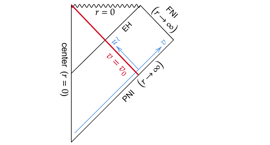
Figure 1: The Penrose diagram of a spherical collapsing null shell spacetime. The red line represents the null shell. Above (below) the red line lies the shell’s exterior (interior), described by the Schwarzschild (Minkowski) geometry. Blue arrows indicate the global $\tilde{u}$ and $v$ coordinates (outside the EH).

The geometry outside the shell (namely at $v>v_{0}$) is Schwarzschild with $M=M_{0}$, while inside the shell ($v<v_{0}$) it is Minkowski ($M=0$). That is, $M=M_{0}\Theta(v-v_{0})$, where $\Theta$ denotes the standard step function. These two different geometries are continuously matched across the shell – that is, the overall metric should be continuous (in appropriate coordinates).

The Schwarzschild geometry is given in double-null Eddington coordinates $(u,v,\theta,\varphi)$ by $ds^{2}=-f\,du\,dv+r^{2}d\Omega^{2}$, where $r$ is now viewed as a function of the coordinates $u,v$ (defined implicitly via the relation $r_{*}(r)$ given above, as $r_{*}=\left(v-u\right)/2$).

As already mentioned, the metric across the thin shell is in principle continuous (provided that one uses appropriate coordinates – which are themselves continuous across the shell, as we do below). In particular, $r$ is necessarily continuous at the shell, and so are the coordinates $v,\theta,\varphi$. Note, however, that if the Eddington coordinate $u$ is used globally (i.e. at both sides), the resultant metric is discontinuous. In particular, $-2g_{uv}$ is equal to $f=1-(2M_{0}/r)\Theta(v-v_{0})$, wherein the step function $\Theta(v-v_{0})$ indicates discontinuity at the shell. To achieve metric continuity, we choose our global ingoing null coordinate $\tilde{u}$ (defined outside the EH) as follows: In the Schwarzschild region outside the shell we set $\tilde{u}\equiv u$; and inside the shell we define $\tilde{u}\left(u\right)$ by simply requiring it to continuously match the aforementioned Schwarzschild’s $u$$(=\tilde{u})$. Explicitly, this continuous $\tilde{u}$ coordinate turns out to be (see (MassarParentani:1996, ; FabbriNavarroSalas:Book, ; AndersonSiahmazginClarkFabbri:2020, ))

$$\tilde{u}(u)\equiv u-4M_{0}\ln\left(\frac{v_{0}-u}{4M_{0}}-1\right)\Theta(v_{0}-v)\,.$$ (1)

The metric is then continuous across the shell, with $g_{\tilde{u}v}$ being $-(1/2)(1-2M_{0}/r)$ at the shell (as approached from both sides). For later use, we also note that inside the shell

$$\frac{du}{d\tilde{u}}=1-\frac{4M_{0}}{v_{0}-u}=1-\frac{2M_{0}}{r(u,v_{0})}\,,\,\,\,\,\,\,\,\,\,\,\,\,(v<v_{0})\,.$$ (2)

Field modes and quantum state.

Our real scalar field $\Phi$ satisfies the field equation $\Box\Phi=0$. We decompose it into normalized mode solutions $\Phi_{\omega lm}(x)$, defined by their asymptotic initial data at past null infinity (PNI):

$$\Phi_{\omega lm}(x)=\frac{1}{r\sqrt{4\pi\omega}}Y_{lm}(\theta,\varphi)\exp(-i\omega v)\,,\,\,\,\,(\text{PNI})$$ (3)

along with the usual regularity condition at $r=0$. Here $Y_{lm}(\theta,\varphi)$ are the spherical harmonics.

The quantum field may then be expressed as

$$\hat{\Phi}(x)=\!\int_{0}^{\infty}\!d\omega\sum_{lm}\left[\Phi_{\omega lm}(x)\hat{a}_{\omega lm}+\Phi_{\omega lm}^{*}(x)\hat{a}_{\omega lm}^{{\dagger}}\right],$$ (4)

where $\hat{a}_{\omega lm}$ and $\hat{a}_{\omega lm}^{\dagger}$ are respectively the annihilation and creation operators for the $\omega lm$ mode. Our quantum state, denoted $|0\rangle$, is taken to be the “in” vacuum state, namely the vacuum state with respect to the mentioned positive-frequency modes $\Phi_{\omega lm}(x)$, obeying $\hat{a}_{\omega lm}|0\rangle=0$ (indicating no excitations originating from PNI).

The fact that $\Box\Phi_{\omega lm}=0$, combined with the metric continuity, implies that the modes $\Phi_{\omega lm}(x)$ are continuous across the shell.

In an entirely Minkowski spacetime (no collapsing shell), both $\left\langle\hat{\Phi}^{2}\right\rangle_{\text{ren}}$ and the RSET trivially vanish everywhere in the vacuum state $|0\rangle$. In our model, spacetime remains Minkowski until the shell emerges from PNI at $v=v_{0}$. By causality, this shell cannot affect physical quantities at earlier $v$ values. Therefore, both $\left\langle\hat{\Phi}^{2}\right\rangle_{\text{ren}}$ and the RSET vanish throughout the shell’s interior, namely at $v<v_{0}$. However, at the shell’s exterior, these quantities generally do not vanish due to the existing curvature. Our goal in this paper is to compute $\left\langle\hat{\Phi}^{2}\right\rangle_{\text{ren}}$ and $\left\langle\hat{T}_{uu}\right\rangle_{\text{ren}}$ at the shell’s Schwarzschild side, that is, at $v\to v_{0}^{+}$.

Computation of $\left\langle\hat{\Phi}^{2}\right\rangle_{\text{ren}}$.

To renormalize $\left\langle\hat{\Phi}^{2}\right\rangle$, at a generic point $x$ in Schwarzschild (or Minkowski), we use the point-splitting procedure:

$$\left\langle\hat{\Phi}^{2}\right\rangle_{\text{ren}}(x)=\lim_{x^{\prime}\to x}\left[G\left(x,x^{\prime}\right)-G_{DS}(x,x^{\prime})\right]\,,$$ (5)

where $G(x,x^{\prime})\equiv\left\langle\hat{\Phi}\left(x\right)\hat{\Phi}\left(x^{\prime}\right)\right\rangle$ and $G_{DS}(x,x^{\prime})$ is the counterterm (DeWittBook:1965, ).

In view of the spherical symmetry, we choose $\theta$-splitting (LeviOriTheta:2016, ). Without loss of generality, we pick our point $x$ to be at $(u,v,\theta=0)$ and $x^{\prime}$ at $(u,v,\theta=\varepsilon)$; hence $\left\langle\hat{\Phi}^{2}\right\rangle_{\text{ren}}(x)$ effectively reduces to $\left\langle\hat{\Phi}^{2}\right\rangle_{\text{ren}}(u,v)$, $G(x,x^{\prime})$ to $G(u,v;\varepsilon)$, and $G_{DS}(x,x^{\prime})$ to $G_{DS}(r;\varepsilon)$, where $r=r(u,v)$ is to be understood. The above equation (5) then reduces to

$$\left\langle\hat{\Phi}^{2}\right\rangle_{\text{ren}}(u,v)=\lim_{\varepsilon\to 0}\left[G(u,v;\varepsilon)-G_{DS}(r;\varepsilon)\right]\,.$$ (6)

This equation applies everywhere in the Schwarzschild region at $v>v_{0}$, and likewise throughout the Minkowski region at $v<v_{0}$.

We now choose a point on the shell, denoted $x_{\text{sh}}$ (at $\theta=0$), with a certain $r$ value denoted $r_{0}$ and a $\tilde{u}$ value (determined by $v_{0}$ and $r_{0}$) denoted $\tilde{u}_{0}$. We wish to compute $\left\langle\hat{\Phi}^{2}\right\rangle_{\text{ren}}(x_{\text{sh}})$ when the point $x_{\text{sh}}$ is approached “from the Schwarzschild side of the shell”. We hereafter use a superscript “$+$” to denote quantities evaluated in the Schwarzschild geometry outside the shell, approaching $x_{\text{sh}}$ (i.e., with $v\to v_{0}^{+}$). Applying Eq. (6) for this purpose, we obtain

$$\left\langle\hat{\Phi}^{2}\right\rangle_{\text{ren}}^{+}(x_{\text{sh}})=\lim_{\varepsilon\to 0}\left[G^{+}(\tilde{u}_{0},v_{0};\varepsilon)-G_{DS}^{+}(r_{0};\varepsilon)\right].$$ (7)

We can now repeat the above procedure approaching from the Minkowski side:

$$\left\langle\hat{\Phi}^{2}\right\rangle_{\text{ren}}^{-}(x_{\text{sh}})=\lim_{\varepsilon\to 0}\left[G^{-}(\tilde{u}_{0},v_{0};\varepsilon)-G_{DS}^{-}(r_{0};\varepsilon)\right]\,,$$ (8)

where the superscript “$-$” refers to quantities evaluated at the Minkowski side of the shell, approaching $x_{\text{sh}}$ (with $v\to v_{0}^{-}$). Note, however, that in view of Eq. (4) the continuity of the field modes $\Phi_{\omega lm}(x)$ at the shell implies the continuity of $G(\tilde{u},v;\varepsilon)$ there, therefore

$$G^{+}(\tilde{u}_{0},v_{0};\varepsilon)=G^{-}(\tilde{u}_{0},v_{0};\varepsilon)\,.$$ (9)

Also, since in our model $\left\langle\hat{\Phi}^{2}\right\rangle$ vanishes throughout $v<v_{0}$ as mentioned above, $\left\langle\hat{\Phi}^{2}\right\rangle_{\text{ren}}^{-}(x_{\text{sh}})$ vanishes and we can trivially replace $\left\langle\hat{\Phi}^{2}\right\rangle_{\text{ren}}^{+}(x_{\text{sh}})$ with $\left\langle\hat{\Phi}^{2}\right\rangle_{\text{ren}}^{+}(x_{\text{sh}})-\left\langle\hat{\Phi}^{2}\right\rangle_{\text{ren}}^{-}(x_{\text{sh}})$. Using Eqs. (7) and (8), and recalling Eq. (9), we then get

$$\left\langle\hat{\Phi}^{2}\right\rangle_{\text{ren}}^{+}(x_{\text{sh}})=-\lim_{\varepsilon\to 0}\left[G_{DS}^{+}(r_{0};\varepsilon)-G_{DS}^{-}(r_{0};\varepsilon)\right].$$ (10)

Note that when computing $\left\langle\hat{\Phi}^{2}\right\rangle_{\text{ren}}^{+}(x_{\text{sh}})$ directly from Eq. (7), the most challenging piece to evaluate is $G^{+}\left(\tilde{u}_{0},v_{0};\varepsilon\right)$, as it requires solving the PDEs for the individual field modes $\Phi_{\omega lm}(x)$, subsequently summing and integrating over all mode contributions. Remarkably, this notoriously demanding quantity is entirely eliminated in Eq. (10), leaving merely the simpler, well-known counterterms.

The explicit form of the $\theta$-splitting counterterm for $\left\langle\hat{\Phi}^{2}\right\rangle$ in Schwarzschild, as a function of the splitting parameter $\varepsilon$, was computed in (LeviOriTheta:2016, ). Its general form is given in Eq. (3.10) therein, in terms of the coefficients $a,c,d$ which are specified in the equation preceding Eq. (4.2). For Schwarzschild with a general mass parameter $M$:

$$G_{DS}(r;\varepsilon)=\hbar\left[\frac{1}{16\pi^{2}r^{2}}\sin^{-2}(\varepsilon/2)-\frac{M}{24\pi^{2}r^{3}}\right]\,.$$

Substituting this expression in Eq. (10) with $M=M_{0}$ for $G_{DS}^{+}$ and $M=0$ for $G_{DS}^{-}$, and setting $r=r_{0}$ in both, the shared $\varepsilon$-dependent term drops out. Our result for $\left\langle\hat{\Phi}^{2}\right\rangle_{\text{ren}}$ at the shell’s external side, in terms of $r_{0}$ (the $r$ value on the shell), is therefore:

$$\left\langle\hat{\Phi}^{2}\right\rangle_{\text{ren}}^{+}(r_{0})=\frac{\hbar}{24\pi^{2}}\,\frac{M_{0}}{r_{0}^{3}}\,.$$ (11)

Generalization to $\left\langle\hat{T}_{uu}\right\rangle_{\text{ren}}$.

Since the shell is parameterized by $\tilde{u}$ (along with $\theta,\varphi$), the continuity of $\Phi_{\omega lm}\left(x\right)$ across the shell implies the continuity of $\Phi_{\omega lm,\tilde{u}}$ there, allowing a natural extension of the $\left\langle\hat{\Phi}^{2}\right\rangle_{\text{ren}}$ analysis to $\left\langle\hat{T}_{\tilde{u}\tilde{u}}\right\rangle_{\text{ren}}$.

The analog of Eq. (5) for the (trace-reversed) RSET is given in Eq. (2.6) in (LeviRSET:2017, ) (which applies to any splitting direction). When reduced to the $uu$ component it reads (recalling that $g_{uu}=0$ and hence $T_{uu}$ equals its trace-reversed counterpart)

$$\left\langle\hat{T}_{uu}\right\rangle_{\text{ren}}(x)=\lim_{x^{\prime}\to x}\left[G_{uu}(x,x^{\prime})-\tilde{L}_{uu}(x,x^{\prime})\right],$$ (12)

where $G_{uu}(x,x^{\prime})\equiv\frac{1}{2}\left\langle\left\{\hat{\Phi}_{,u}(x),\hat{\Phi}_{,u}(x^{\prime})\right\}\right\rangle$, $\left\{...\right\}$ denotes anti-commutation, and $\tilde{L}_{\mu\nu}(x,x^{\prime})$ is the “coordinate-based explicit counterterm” obtained from Christensen’s counterterm $C_{\mu\nu}(x,x^{\prime})$ as described in Eq. (2.5) in (LeviRSET:2017, ).

We shall again use $\theta$-splitting, placing $x$ at $\theta=0$ and $x^{\prime}$ at $\theta=\varepsilon$. The $T_{uu}$ analog of Eq. (6) now reads

$$\left\langle\hat{T}_{uu}\right\rangle_{\text{ren}}(u,v)=\lim_{\varepsilon\to 0}\left[G_{uu}(u,v;\varepsilon)-\tilde{L}_{uu}(r;\varepsilon)\right]\,.$$ (13)

We consider $\left\langle\hat{T}_{uu}\right\rangle_{\text{ren}}$ as the point $x_{\text{sh}}$ is approached from either the Minkowski or Schwarzschild side (i.e., $x\to x_{\text{sh}}^{\pm}$). We obtain the $\left\langle\hat{T}_{uu}\right\rangle_{\text{ren}}$ analog of Eqs. (7) and (8), which we collectively write as

$$\left\langle\hat{T}_{uu}\right\rangle_{\text{ren}}^{\pm}(x_{\text{sh}})=\lim_{\varepsilon\to 0}\left[G_{uu}^{\pm}(\tilde{u}_{0},v_{0};\varepsilon)-\tilde{L}_{uu}^{\pm}(r_{0};\varepsilon)\right].$$ (14)

We would again like to subtract the “$-$” version of $\left\langle\hat{T}_{uu}\right\rangle_{\text{ren}}$ from its “$+$” version, to eliminate the $G_{uu}$ terms altogether. Recall, however, that it is $\hat{\Phi}_{,\tilde{u}}$ that is continuous across the shell, not $\hat{\Phi}_{,u}$. Therefore, $G_{uu}$ is not continuous at the shell, whereas $G_{\tilde{u}\tilde{u}}$ is. This motivates transforming Eq. (14) from $u$ to $\tilde{u}$, via multiplication by $(du/d\tilde{u})^{2}$:

$$\left\langle\hat{T}_{\tilde{u}\tilde{u}}\right\rangle_{\text{ren}}^{\pm}(x_{\text{sh}})=\lim_{\varepsilon\to 0}\left[G_{\tilde{u}\tilde{u}}^{\pm}(\tilde{u}_{0},v_{0};\varepsilon)-\tilde{L}_{\tilde{u}\tilde{u}}^{\pm}(r_{0};\varepsilon)\right],$$ (15)

where $G_{\tilde{u}\tilde{u}}(x,x^{\prime})\equiv\frac{1}{2}\left\langle\left\{\hat{\Phi}_{,\tilde{u}}(x),\hat{\Phi}_{,\tilde{u}}(x^{\prime})\right\}\right\rangle$ and

$$\tilde{L}_{\tilde{u}\tilde{u}}^{\pm}(r_{0};\varepsilon)\equiv\left(\frac{du}{d\tilde{u}}\right)^{2}\tilde{L}_{uu}^{\pm}(r_{0};\varepsilon)\,.$$

Recalling Eq. (2) (and $du/d\tilde{u}=1$ at $v>v_{0}$), we get

$$\tilde{L}_{\tilde{u}\tilde{u}}^{+}(r_{0};\varepsilon)=\tilde{L}_{uu}^{+}(r_{0};\varepsilon)\,,\,\,\,\,\tilde{L}_{\tilde{u}\tilde{u}}^{-}(r_{0};\varepsilon)=f_{0}^{2}\tilde{L}_{uu}^{-}$$ (16)

where $f_{0}\equiv 1-2M_{0}/r_{0}$.

From this point, the analysis proceeds in full analogy with the above treatment of $\left\langle\hat{\Phi}^{2}\right\rangle_{\text{ren}}$. First, recalling that $\left\langle\hat{T}_{\tilde{u}\tilde{u}}\right\rangle_{\text{ren}}$ (like $\left\langle\hat{T}_{uu}\right\rangle_{\text{ren}}$) vanishes in the Minkowski region,

$$\left\langle\hat{T}_{\tilde{u}\tilde{u}}\right\rangle_{\text{ren}}^{+}(x_{\text{sh}})=\left\langle\hat{T}_{\tilde{u}\tilde{u}}\right\rangle_{\text{ren}}^{+}(x_{\text{sh}})-\left\langle\hat{T}_{\tilde{u}\tilde{u}}\right\rangle_{\text{ren}}^{-}(x_{\text{sh}})\,.$$ (17)

Next, the continuity of $G_{\tilde{u}\tilde{u}}(x,x^{\prime})$ across the shell implies that $G_{\tilde{u}\tilde{u}}^{+}(\tilde{u}_{0},v_{0};\varepsilon)=G_{\tilde{u}\tilde{u}}^{-}(\tilde{u}_{0},v_{0};\varepsilon)$, allowing us to rewrite Eq. (15) as

$$\left\langle\hat{T}_{\tilde{u}\tilde{u}}\right\rangle_{\text{ren}}^{\pm}(x_{\text{sh}})=\lim_{\varepsilon\to 0}\left[G_{\tilde{u}\tilde{u}}(\tilde{u}_{0},v_{0};\varepsilon)-\tilde{L}_{\tilde{u}\tilde{u}}^{\pm}(r_{0};\varepsilon)\right]\,,$$

and substituting it in Eq. (17) we obtain

$$\left\langle\hat{T}_{\tilde{u}\tilde{u}}\right\rangle_{\text{ren}}^{+}(x_{\text{sh}})=-\lim_{\varepsilon\to 0}\left[\tilde{L}_{\tilde{u}\tilde{u}}^{+}(r_{0};\varepsilon)-\tilde{L}_{\tilde{u}\tilde{u}}^{-}(r_{0};\varepsilon)\right]\,.$$

At this stage, it becomes convenient to re-express this equation in terms of the Eddington $u$ coordinate instead of $\tilde{u}$, using Eq. (16) and recalling that $\left\langle\hat{T}_{\tilde{u}\tilde{u}}\right\rangle_{\text{ren}}^{+}=\left\langle\hat{T}_{uu}\right\rangle_{\text{ren}}^{+}$:

$$\left\langle\hat{T}_{uu}\right\rangle_{\text{ren}}^{+}(x_{\text{sh}})=-\lim_{\varepsilon\to 0}\left[\tilde{L}_{uu}^{+}(r_{0};\varepsilon)-f_{0}^{2}\tilde{L}_{uu}^{-}(r_{0};\varepsilon)\right]\,.$$ (18)

Both $\tilde{L}_{uu}^{+}(r_{0};\varepsilon)$ and $\tilde{L}_{uu}^{-}(r_{0};\varepsilon)$ are obtained from the basic $\theta$-splitting counterterm $\tilde{L}_{uu}(r;\varepsilon)$ for the Schwarzschild metric of general mass parameter $M$, by substituting the appropriate mass parameter ($M_{0}$ or $0$) and setting $r=r_{0}$. The expression in square brackets in Eq. (18) then becomes

$$\left(\tilde{L}_{uu}(r_{0};\varepsilon)|_{M=M_{0}}\right)-f_{0}^{2}\left(\tilde{L}_{uu}(r_{0};\varepsilon)|_{M=0}\right)\,.$$ (19)

The mentioned basic Schwarzschild’s counterterm $\tilde{L}_{uu}(r;\varepsilon)$ was presented in Sec. 1 of the supplemental material of (FluxesRN:2020, ) (setting $Q=0$). It reads

$$\tilde{L}_{uu}(r;\varepsilon)=\hbar\left[\frac{f^{2}}{64\pi^{2}r^{4}}\sin^{-2}(\varepsilon/2)+e_{uu}\right]\,,$$ (20)

where $e_{uu}=-3Mf{}^{2}/160\pi^{2}r^{5}$. Substituting this expression into Eq. (19), the two terms $\propto\sin^{-2}(\varepsilon/2)$ cancel out, leaving only the $\propto e_{uu}$ contribution – which is independent of $\varepsilon$ (and vanishes in the $M=0$ case). This yields our final result for the outflux density at the shell’s external side (at a point where $r=r_{0}$):

$$\left\langle\hat{T}_{uu}\right\rangle_{\text{ren}}^{+}\left(r_{0}\right)=\hbar\frac{3M_{0}}{160\pi^{2}r_{0}^{5}}\left(1-\frac{2M_{0}}{r_{0}}\right)^{2}\,.$$ (21)

Discussion.

The result (21) reveals that as the shell approaches the EH, the outflux density $\left\langle\hat{T}_{uu}\right\rangle_{\text{ren}}^{+}$ emerging from the shell vanishes quadratically with the remaining distance $r_{0}-2M_{0}$. This vanishing rate ensures the regularity of the Kruskal-based outflux density $\left\langle\hat{T}_{UU}\right\rangle_{\text{ren}}^{+}$ at the EH.

Our result clarifies the origin of the Hawking outflux (at least in the collapsing null shell case). Consider the evolution of $F=4\pi r^{2}\left\langle\hat{T}_{uu}\right\rangle_{\text{ren}}$ along an outgoing null ray $u=\text{const}\equiv u_{0}\gg M_{0}$. This geodesic leaves the shell at $r=r_{0}\approx 2M_{0}$ and propagates towards FNI. Eq. (21) implies that the outflux emerging from the shell, $F^{+}\left(r_{0}\right)\equiv 4\pi r_{0}^{2}\left\langle\hat{T}_{uu}\right\rangle_{\text{ren}}^{+}\left(r_{0}\right)$, is negligibly small for such a geodesic; whereas when the geodesic approaches the weak-field region ($r\gg M_{0}$), $F$ has already reached its asymptotic value $F_{H}$. That is, the evolution of $F$ along the outgoing null ray from $F^{+}\left(u_{0}\right)\approx 0$ (at the shell) to $F_{H}$ (at FNI) occurs, gradually, as the ray traverses the strong-field region. This designates scenario (i), presented in the Introduction, as the correct physical description.

Multiplying Eq. (21) by $4\pi r_{0}^{2}$, one finds that at $r_{0}^{\text{max}}=(10/3)M$ the mentioned outflux $F^{+}\left(r_{0}\right)$ reaches a maximum value of $\left(81/250000\pi\right)\hbar M^{-2}\approx 1.031\times 10^{-4}\hbar M^{-2}$. Interestingly, this value exceeds the known (Elster:1983, ) Hawking outflux in Schwarzschild, $F_{H}\approx 7.44\times 10^{-5}\hbar M^{-2}$. This suggests that perhaps the outflux $F$ evolves nonmonotonically (with $r$) along the outgoing null geodesic emanating from the shell at $r_{0}^{\text{max}}$. This should not be too surprising, as such nonmonotonic behavior of the outflux is actually observed already in the Unruh state in Schwarzschild (see Appendix).

As noted in footnote [33] , our computational method inherently involves an interchange of two limits, which we have not attempted to rigorously justify. A deeper mathematical investigation of this issue of interchangeability would be desired, although such an analysis may be rather challenging. Generally speaking, the computation of renormalized quantities in BH backgrounds may typically involve several limits, including: (i) the coincidence limit $x^{\prime}\to x$, (ii) an infinite mode sum (if mode decomposition is used), and (iii) in some cases, an additional limit of approaching a desired destination point $x_{\text{dest}}$ (e.g., when a direct computation at $x_{\text{dest}}$ is problematic or challenging). Basically, the required order of limits is: first, performing the mode sum (if relevant); second, taking the coincidence limit (after counterterm subtraction); and finally, approaching the destination point (when applicable). However, in various concrete computational schemes, some of these limits are often interchanged. For instance, in the “Pragmatic Mode-sum Regularization” method (LeviOriT:2015, ; LeviOriRSET:2016, ), the mode sum and the coincidence limit are effectively interchanged. Nevertheless, results obtained through this method have been separately confirmed in multiple cases (LeviOriT:2015, ; LeviOriRSET:2016, ; LeviRSET:2017, ; LeviEilonOriMeent:2017, ; SchLanir:2018, ; KerrIH:2022, ; t-splitKerr:2024, ).

In the present analysis, the coincidence and the $x\to x_{\text{dest}}$ limits were implicitly interchanged. This situation somewhat resembles the flux computation at a Kerr BH’s inner horizon in Ref. (KerrIH:2022, ), where the mode sum and the limit $r\to r_{-}$ were effectively interchanged: while $\left\langle T_{vv}\right\rangle_{\text{ren}}^{-}$ was defined there as $\lim_{r\to r_{-}}\left\langle T_{vv}\right\rangle_{\text{ren}}\left(r\right)$ (mainly because Unruh’s field modes are literally ill-defined at $r=r_{-}$), in practice this $r\to r_{-}$ limit was applied to the individual mode contributions before summation and integration. The validity of the results in that case was nevertheless independently confirmed by applying $t$-splitting at a set of points reaching very close to $r_{-}$ (t-splitKerr:2024, ). Similarly in our case, it would be highly beneficial to conduct an independent computation of the outflux emerging from the shell (e.g. by using the methods developed in Refs. (AndersonSiahmazginClarkFabbri:2020, ; SiahmazgiAndersonClarkFabbri:2021, )), to provide a robust cross-check of our result (21).

It may also be interesting – and physically important – to replace the scalar field with the more realistic electromagnetic field.

.1 Appendix

As mentioned in the Discussion, the function $F^{+}\left(r_{0}\right)$ – representing the outflux on the Schwarzschild side of the shell as a function of $r_{0}$ (namely the area coordinate $r$ on the shell) – attains a maximum value $\approx 1.031\times 10^{-4}\hbar M^{-2}$ at $r_{0}^{\text{max}}=(10/3)M$ that exceeds the known (Elster:1983, ) Hawking radiation outflux $F_{H}\approx 7.44\times 10^{-5}\hbar M^{-2}$. This fact may suggest a nonmonotonic dependence of the outflux $F$ on $r$ along the outgoing null geodesic emerging from the shell at $r_{0}^{\text{max}}$ (as well as along its neighboring outgoing null geodesics). To put this suggested behavior in a wider context, it may be useful to compare it with the $r$-dependence of the outflux in the Unruh state in Schwarzschild, denoted $F^{U}\left(r\right)\equiv 4\pi r^{2}\left\langle\hat{T}_{uu}\right\rangle_{\text{ren}}^{U}\left(r\right)$ (here, the superscript $"U"$ denotes the Unruh state). Due to the stationarity in this case, $F^{U}$ is a function of $r$ alone, satisfying $\lim_{r\to\infty}F^{U}(r)=F_{H}$.

Using the results for $\left\langle\hat{T}_{t}^{t}\right\rangle_{\text{ren}}^{U}$, $\left\langle\hat{T}_{r}^{r}\right\rangle_{\text{ren}}^{U}$ and $\left\langle\hat{T}_{t}^{r}\right\rangle_{\text{ren}}^{U}$ of Ref. (LeviRSET:2017, ) (see, in particular, Fig. 4 therein), we construct $\left\langle\hat{T}_{uu}\right\rangle_{\text{ren}}^{U}\left(r\right)$ and then $F^{U}\left(r\right)$, and explore the latter’s dependence on $r$. As expected from regularity, we find that it behaves as $\left(1-2M/r\right)^{2}$ near the EH (similar to $F^{+}\left(r\right)$, though with a different prefactor). Then, as $r$ increases outwards, the Unruh outflux does not grow monotonically toward $F_{H}$. Instead, it initially increases to a maximum at $r\approx 4.55M$, see Fig. 2. Then, it gradually decreases toward $F_{H}$ as $r\to\infty$.

Given this behavior in the Unruh state, it is not too surprising if the outflux along outgoing null geodesics in the collapsing-shell spacetime exhibits a similar nonmonotonic trend.

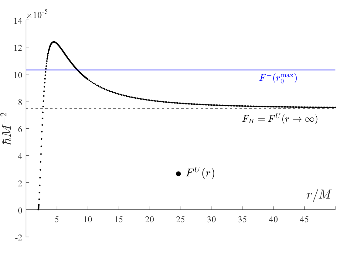
Figure 2: The black dotted curve represents the Unruh outflux, $F^{U}=4\pi r^{2}\left\langle T_{uu}\right\rangle_{\text{ren}}^{U}$, as a function of $r$, asymptotically approaching $F_{H}$ which is indicated by the horizontal dashed line. The horizontal blue line marks the maximum value of $F^{+}\left(r_{0}\right)$, the outflux emerging from the shell. Notably, this value is greater than $F_{H}$ but still smaller than the peak of $F^{U}\left(r\right)$.

References

- (1) S. W. Hawking, Black hole explosions?, Nature 248, 30 (1974).
- (2) S. W. Hawking, Particle creation by black holes, Comm. Math. Phys. 43, 199 (1975).
- (3) P. Chen, W. G. Unruh, C. H. Wu, and D. H. Yeom, Pre-hawking radiation cannot prevent the formation of apparent horizon, Phys. Rev. D 97(6), 064045 (2018).
- (4) P. C. W. Davies, On the Origin of Black Hole Evaporation Radiation, Proc. R. Soc. Lond. A 351, 129 (1976).
- (5) H. Kawai, Y. Matsuo and Y. Yokokura, A Self-consistent Model of the Black Hole Evaporation, Int. J. Mod. Phys. A 28, 1350050 (2013).
- (6) P. M. Ho, Comment on Self-Consistent Model of Black Hole Formation and Evaporation, JHEP 1508, 096 (2015).
- (7) H. Kawai and Y. Yokokura, Interior of Black Holes and Information Recovery, Phys. Rev. D 93(4), 044011 (2016).
- (8) P. M. Ho, The Absence of Horizon in Black-Hole Formation, Nucl. Phys. B 909, 394 (2016).
- (9) D. Maskalaniec and B. Sikorski, Hawking radiation far away from the event horizon, arXiv:2409.11021v1 [gr-qc] (2024).
- (10) L. Mersini-Houghton, Backreaction of Hawking Radiation on a Gravitationally Collapsing Star I: Black Holes?, Phys. Lett. B 738, 61 (2014).
- (11) L. Mersini-Houghton, Back-reaction of the Hawking radiation flux on a gravitationally collapsing star II, arXiv:1409.1837 [hep-th] (2014).
- (12) V. Baccetti, R. B. Mann and D. R. Terno, Role of evaporation in gravitational collapse, arXiv:1610.07839 [gr-qc] (2016).
- (13) V. Baccetti, R. B. Mann and D. R. Terno, Horizon avoidance in spherically-symmetric collapse, arXiv:1703.09369 [gr-qc] (2017).
- (14) V. Baccetti, R. B. Mann and D. R. Terno, Do event horizons exist?, Int. J. Mod. Phys. D 26, 743008 (2017).
- (15) P. R. Anderson, S. G. Siahmazgi, R. D. Clark, and A. Fabbri, Method to compute the stress-energy tensor for a quantized scalar field when a black hole forms from the collapse of a null shell, Phys. Rev. D 102, 125035 (2020).
- (16) S. G. Siahmazgi, P. R. Anderson, R. D. Clark, and A. Fabbri, Stress-energy Tensor for a Quantized Scalar Field in a Four-Dimensional Black Hole Spacetime that Forms From the Collapse of a Null Shell, In The Sixteenth Marcel Grossmann Meeting on Recent Developments in Theoretical and Experimental General Relativity, Astrophysics and Relativistic Field Theories: Proceedings of the MG16 Meeting on General Relativity; 5–10 July 2021, pp. 1265-1274.
- (17) S. Massar and R. Parentani, From vacuum fluctuations to radiation. II. Black holes, Phys. Rev. D 54, 7444 (1996).
- (18) A. Fabbri and J. Navarro-Salas, Modeling black hole evaporation, Imperial College Press, London, UK, 2005.
- (19) B. S. DeWitt, Dynamical Theory of Groups and Fields (Gordon and Breach, New York, 1965).
- (20) A. Levi and A. Ori, Mode-sum regularization of in the angular-splitting method, Phys. Rev. D. 94, 044054 (2016).
- (21) P. Candelas, Vacuum polarization in Schwarzschild spacetime, Phys. Rev. D. 21, 2185 (1980).
- (22) A. Levi, Renormalized stress-energy tensor for stationary black holes, Phys. Rev. D. 95, 025007 (2017).
- (23) N. Zilberman, A. Levi and A. Ori, Quantum Fluxes at the Inner Horizon of a Spherical Charged Black Hole, Phys. Rev. Lett. 124, 171302 (2020).
- (24) T. Elster, vacuum polarization near a black hole creating particles, Phys. Lett. A 94(5), 205 (1983).
- (25) A. Levi and A. Ori, Pragmatic mode-sum regularization method for semiclassical black-hole spacetimes, Phys. Rev. D. 91, 104028 (2015).
- (26) A. Levi and A. Ori, Versatile Method for Renormalized Stress-Energy Computation in Black-Hole Spacetimes, Phys. Rev. Lett. 117, 231101 (2016).
- (27) N. Zilberman, M. Casals, A. Ori and A. C. Ottewill, Quantum fluxes at the inner horizon of a spinning black hole, Phys. Rev. Lett. 129, 261102 (2022).
- (28) A. Levi, E. Eilon, A. Ori and M. van de Meent, Renormalized Stress-Energy Tensor of an Evaporating Spinning Black Hole, Phys. Rev. Lett. 118, 141102 (2017).
- (29) A. Lanir, A. Levi, and A. Ori, Mode-sum renormalization of for a quantum scalar field inside a Schwarzschild black hole, Phys. Rev. D. 98, 084017 (2018).
- (30) N. Zilberman, M. Casals, A. Levi, A. Ori and A. C. Ottewill, Computation of and quantum fluxes at the polar interior of a spinning black hole, arXiv:2409.17464 [gr-qc] (2024).