The Uncertainty of Machine Learning Predictions in Asset Pricing

Abstract

Machine learning in asset pricing typically predicts expected returns as point estimates, ignoring uncertainty. We develop new methods to construct forecast confidence intervals for expected returns obtained from neural networks. We show that neural network forecasts of expected returns share the same asymptotic distribution as classic nonparametric methods, enabling a closed-form expression for their standard errors. We also propose a computationally feasible bootstrap to obtain the asymptotic distribution. We incorporate these forecast confidence intervals into an uncertainty-averse investment framework. This provides an economic rationale for shrinkage implementations of portfolio selection. Empirically, our methods improve out-of-sample performance.

1 Introduction

Pension funds, wealth advisors, and hedge funds worldwide employ predictive methods to forecast asset returns and construct optimal portfolios that aim to maximize client returns. Recently, machine learning (ML) models have gained prominence in predicting asset returns, selecting portfolios, and estimating stochastic discount factors, with significant success in these areas. ML techniques, by capturing complex and nonlinear relationships in financial data, are particularly well-suited for enhancing portfolio management decisions. For example, within the mean-variance portfolio framework, ML methods are increasingly used to estimate expected returns and (co)variances, often leading to more effective portfolio allocations. The literature consistently demonstrates the effectiveness of machine learning in these and other applications (e.g., Gu, Kelly, and Xiu (2020); Bianchi, Büchner, and Tamoni (2021); Cong, Tang, Wang, and Zhang (2021); Kelly, Malamud, and Zhou (2021); Patton and Weller (2022); Didisheim, Ke, Kelly, and Malamud (2023); Filipovic and Schneider (2024)).

Despite the success of machine learning in asset pricing, existing literature typically treats ML predictions as point estimates and conducts asset pricing analyses as if they were true values, overlooking the associated uncertainty. This is surprising, given that uncertainty about input parameters is widely acknowledged as critical in portfolio selection (e.g., DeMiguel, Garlappi, and Uppal (2009)), and Garlappi, Uppal, and Wang (2007) show that incorporating forecast uncertainty in mean-variance portfolio allocation leads to distinct economic insights. However, quantifying prediction uncertainty in ML forecasts, particularly with neural networks, remains a complex challenge, limiting their broader application in asset pricing. This paper addresses this gap by rigorously quantifying uncertainty in ML predictions and incorporating it into portfolio selection, specifically by constructing forecast confidence intervals (FCIs) for return predictions from neural networks.

We provide two methods for constructing forecast confidence intervals: one based on closed-form approximations and the other on the bootstrap. A key theoretical contribution of this paper is our proof that ML-based forecast methods exhibit an asymptotic distribution independent of the specific ML model used to generate the forecast. For example, the asymptotic distribution of neural network forecasts is not specific to neural networks. This implies that, under appropriate technical conditions, simpler machine learning methods—such as Fourier series, particularly those with closed-form estimators—can be utilized to construct confidence intervals. These intervals can be applied to algorithmically more complex machine learning estimators, whose confidence intervals would otherwise be intractable. Building on this insight, we derive an analytic formula for the ML forecast standard error, which is straightforward to calculate and paves the way for constructing the FCI.

For the second method, we propose a novel $k$-step bootstrap approach to simulating the asymptotic distribution of the ML forecast. This method overcomes the substantial computational burden associated with conventional bootstrap procedures, which require repeatedly fully training multiple neural networks from scratch. In contrast, the $k$-step bootstrap, originally developed by Davidson and MacKinnon (1999) and Andrews (2002), starts with the previously trained neural network and retrains it for additional $k$ steps on a bootstrap resample. Through the $k$-step method, a pre-trained neural network can achieve a high level of training accuracy as quantified by the validity of the FCIs’ coverages, even if $k$ is relatively small. inline,linecolor=red,backgroundcolor=red!25,bordercolor=red,]revisit the sentence above

We verify that both methods give correct asymptotic coverage probabilities for ML forecasts of expected returns, while effectively addressing cross-sectional dependence. Empirically, the two methods produce qualitatively similar results. We recommend that researchers compare the two as robustness check. In some applications, it may also be prudent to follow a conservative approach and use the larger of the two standard errors. Furthermore, through extensive simulations, we demonstrate that alternative bootstrap approaches, such as bootstrapping across assets or jointly across assets and time series, fail to produce a valid forecast confidence interval for machine learning forecasts.

In the second part of the paper, we apply our methods for quantifying estimation uncertainty to two standard problems in portfolio selection. We adopt the view of an uncertainty-averse (UA) investor. In the first application, we build on the framework introduced by Garlappi et al. (2007): we treat the expected return in the classic mean-variance optimization problem as an unknown parameter varying within a confidence interval. Then, we find the optimal portfolio weights for the worst-case scenario of the mean-variance utility, varying the mean within the given interval. Extending the characterization by Garlappi et al. (2007) to the machine learning context, we apply the proposed neural network FCI to forecast the expected return of the UA-portfolio. We show that the solution can be formulated as an $\ell_{1}$-penalized regression problem. Our results establish that portfolio weights exhibit a “non-participation” region for risky assets, meaning an uncertainty-averse investor may choose not to invest in a risky asset if uncertainty about the asset’s expected value exceeds a certain level. In addition, this region expands as the investor’s uncertainty about the expected value increases. In contrast, the non-participation region is not present in the standard mean-variance approach which treats the expected returns as known. This insight offers a clear rationale for employing shrinkage approaches in portfolio selection, as developed by Ao, Li, and Zheng (2019) and Kozak, Nagel, and Santosh (2020). Empirically, the behavior of UA-portfolio of individual stocks aligns closely with our theoretical characterization, and generates higher Sharpe ratios than benchmarks that disregard forecast uncertainty.

In our second application, we focus on selecting assets with statistically significantly positive expected returns and constructing long-only portfolios. This exercise is particularly relevant for mutual funds, which do not employ short positions and thus face exactly this challenge of building long-only portfolios. The forecast confidence interval facilitates the selection of individual securities with significantly positive expected returns while controlling the false discovery rate, thereby mitigating the multiple testing problem as documented by Barras, Scaillet, and Wermers (2010) and Harvey and Liu (2020). Empirically, our long-only investment strategy, which accounts for forecast uncertainty, yields higher out-of-sample average returns and similar standard deviations compared to benchmark methods that select assets without considering forecast uncertainty. In addition, it yields economically significant alphas when regressing the returns on various risk factors.

Our result holds in a setting where the machine learning model is not over-parameterized. Recently, Kelly et al. (2021) and Didisheim et al. (2023) derive results about the out-of-sample properties of portfolios in the context of overparameterized models where the number of parameters far exceeds the sample size. They show the interesting virtue of complexity in asset pricing models. Developing forecast confidence intervals in the virtue of complexity regime is an important question which we leave for future research.

Related Literature

The literature on machine learning in asset pricing has grown rapidly in recent years, such as Kelly, Pruitt, and Su (2019); Kozak, Nagel, and Santosh (2020); Freyberger, Neuhierl, and Weber (2020); Chen, Pelger, and Zhu (2020); Baba-Yara, Boyer, and Davis (2022) and Li, Rossi, Yan, and Zheng (2024). Recently, several papers in asset pricing have made progress in the theoretical analysis of machine learning predictions. Fan, Ke, Liao, and Neuhierl (2022) and Jagannathan, Liao, and Neuhierl (2023) propose the so-called “period-by-period” ML and developed the FCI around the forecast indices, which relies on estimating latent risk factors. Period-by-period learning requires training the machine learning model each period. In this paper, we instead focus exclusively on the popular “pooled machine learning” approach, which is the most common in forecasting applications and does not involve estimating factors.

Allena (2021) is one of the first papers in asset pricing that formally develops confidence intervals for risk premia predicted using machine learning. He proposes a Bayesian ML approach that flexibly draws from posterior distributions of the predicted risk premia and demonstrates that it successfully yields a confidence-based strategy with insightful economic interpretations. The Bayesian approach leverages the fact that posterior distributions, deduced from properly specified priors, can provide valid confidence intervals. In this paper, we take a different approach. In particular, we do not pursue Bayesian estimation. One of the two methods we develop for the forecast confidence interval is based on a derived analytic formula for the ML standard error. Meanwhile, we move to expand the insights obtained by Allena (2021) and Garlappi et al. (2007). In the context of portfolio selection under uncertainty aversion, we show that machine learning confidence intervals lead to qualitatively different investment behavior relative to the standard mean-variance model.

Another strand of literature in asset pricing studies model uncertainty (e.g., Avramov (2002); Anderson and Cheng (2016); Bianchi et al. (2024)). In this line of research, no stance is taken on the “correct model,” as the goal is often to achieve robust portfolio allocations and predictions via Bayesian model averaging. Researchers therefore usually specify a probability distribution over the different models but do not derive the forecast uncertainty within a given model.

In theoretical econometrics, research on machine learning uncertainty is still at a very early stage. There are, however, few papers that rigorously develop the forecast standard error in the i.i.d. setting. In a seminal paper, Chen and White (1999) set the stage for a rigorous analysis of the distributional properties of neural network predictions. In the field of econometric program evaluation, there is a popular method known as “doubly robust ML inference”, which aims to develop asymptotic confidence intervals for some structural parameters in econometric models (e.g., Chernozhukov, Chetverikov, Demirer, Duflo, Hansen, Newey, and Robins (2018)). These methods develop sophisticated procedures that require so-called orthogonal moment conditions and cross-fitting, which are quite different from the typical implementation of ML models in asset pricing. In addition, both approaches rely on the assumption of i.i.d. (or weakly dependent) data, which is invalid in asset pricing due to the strong cross-sectional dependence driven by common risk factors. This dependence is at the heart of the theoretical challenge in asset pricing. This paper proposes new approaches that explicitly account for this dependence and develops forecast confidence intervals with frequentist guarantees.

2 Machine Learning Forecast Confidence Intervals

2.1 The Model

Consider the excess return of a portfolio:

$$z_{t+1}=\sum_{i=1}^{N}w_{i}y_{i,t+1},$$

where $y_{i,t+1},i=1,...,N$ denote the excess return for base asset $i$ from $t$ to $t+1$, relative to the risk-free rate. The portfolio weights $w_{i}$ are assumed to be known at time $t$, but they may vary over time. This contains the special case of an individual asset, i.e., $z_{t+1}=y_{1,t+1}$, or a broad market index. At period $T$, the objective is to forecast the expected excess return of the portfolio:

$$z_{T+1|T}=\mathbb{E}(z_{T+1}|\mathcal{F}_{T})$$

where $\mathcal{F}_{T}$ denotes the information set up to time $T$. To do so, researchers observe a matrix of asset-specific characteristics (features), $x_{t-1}=(x_{1,t-1},...,x_{N,t-1}),$ where $x_{i,t-1}$ is an $d$-dimensional vector of characteristics for asset $i$ at time $t-1$, such as momentum, volatility, financial liabilities. In this setting, machine learning regression, e.g. Gu et al. (2020); Bianchi et al. (2021) have become a very successful and popular methodology to obtain point predictions. ML regressions build on the nonparametric model,

$$y_{i,t}=g(x_{i,t-1})+e_{i,t}$$

with an unknown function $g(\cdot):\mathbb{R}^{d}\to\mathbb{R}$, where $e_{i,t}$ is the error term. The unknown function is learned by pooling all observed data (cross-sectionally and over time) and solving a least squares problem:

$$\widehat{g}(\cdot)=\arg\min_{g\in\mathcal{G}}\sum_{i=1}^{N}\sum_{t=1}^{T}(y_{i,t}-g(x_{i,t-1}))^{2},$$ (2.1)

where the optimal solution is searched for in a function space $\mathcal{G}$ that typically corresponds to a specific machine learning method. Once $\widehat{g}(\cdot)$ has been computed, the expected excess return is predicted by plugging in the most recent characteristic $x_{i,T}$ and constructing a portfolio:

$$\widehat{z}_{T+1|T}:=\sum_{i=1}^{N}w_{i}\widehat{g}(x_{i,T}).$$ (2.2)

This approach is widely used in both academic research and industry applications, making it the primary forecasting method analyzed in this paper.

The choice of the function space $\mathcal{G}$ corresponds to the specific ML method to forecast excess returns. For example, neural networks, random forests, boosted regression trees, or random feature regressions give rise to different $\mathcal{G}$’s. For the purpose of deriving confidence intervals, we focus on two types of machine learning methods,

$$\mathcal{G}=\text{either }\mathcal{G}_{\operatorname{DNN}}\text{ or }\mathcal{G}_{B}.$$

Here $\mathcal{G}_{\operatorname{DNN}}$ corresponds to the use of deep neural network (DNN) functions, which is a collection of all possible neural network functions with a predetermined architecture — specifying the width and depth of the layers and the activation functions for each neuron. Then by minimizing (2.1), we find the optimal neuron biases and weights so that the neural network function $\widehat{g}(\cdot)$ optimally fits the in-sample data.

Alternatively, the more classic nonparametric regression gives rise to an alternative specification $\mathcal{G}=\mathcal{G}_{B}$, which uses a set of basis functions: $\Phi(x)=(\phi_{1}(x),...,\phi_{J}(x))$ such as the Fourier basis. Then, (2.1) searches for the optimal function within a simpler space:

$$\mathcal{G}_{B}=\{\Phi(x)^{\prime}\theta:\theta\in\mathbb{R}^{J}\},$$

and the function $\widehat{g}(\cdot)$ is estimated by finding the best combination of the basis functions.

The crucial distinction between $\mathcal{G}_{\operatorname{DNN}}$ and $\mathcal{G}_{B}$ is that the estimators in $\mathcal{G}_{B}$ admit a closed-form representation, whereas $\mathcal{G}_{\operatorname{DNN}}$ does not. However, $\mathcal{G}_{\operatorname{DNN}}$ is more appealing in predicting expected returns in asset pricing leveraging the advantages of sophisticated machine learning methods, as documented in Gu et al. (2020) and Bianchi et al. (2021). The objective of this paper is to construct forecast confidence intervals for predictions made with neural networks $\mathcal{G}_{\operatorname{DNN}}$, but it will soon become clear that $\mathcal{G}_{B}$ also plays an important role in our construction. Throughout, we refer to $\mathcal{G}_{B}$ as the “closed-form ML”, such as Fourier series regressions, B-Splines – which are more classic nonparametric regression models.

Despite the great popularity and empirical success of machine learning predictions, little work has been devoted to understanding the structure and sources of predictability. However, understanding the structure of the prediction, $\widehat{z}_{T+1|T}$, is crucially important to quantifying the prediction uncertainty. Recently, Fan et al. (2022) provide a thorough analysis by bridging between the machine learning model and factor models. They suppose that excess returns follow a conditional factor model (also see Gagliardini, Ossola, and Scaillet (2016); Zaffaroni (2019)):

$$y_{i,t}=\alpha_{i,t-1}+\beta_{i,t-1}^{\prime}f_{t}+u_{i,t}$$

where $\alpha_{i,t-1}$ and $\beta_{i,t-1}$ are respectively the “alpha” and “beta” of the asset, $f_{t}$ is the set of (possibly latent) risk factors, and $u_{i,t}$ is the idiosyncratic return. In addition, suppose characteristics are informative about factor loadings (betas) and mispricing (alpha), i.e., there are functions $g_{\alpha}$ and $g_{\beta}$ so that we can rewrite alpha and beta as:

$$\alpha_{i,t-1}=g_{\alpha}(x_{i,t-1}),\quad\beta_{i,t-1}=g_{\beta}(x_{i,t-1}).$$

We can thus rewrite the asset pricing model as

$$y_{i,t}=g_{\alpha}(x_{i,t-1})+g_{\beta}(x_{i,t-1})^{\prime}\mathbb{E}f_{t}+g_{\beta}(x_{i,t-1})^{\prime}v_{t}+u_{i,t},$$ (2.3)

where $v_{t}:=f_{t}-\mathbb{E}f_{t}$. Both $v_{t}$ and $u_{i,t}$ are mean-zero processes contributing to the error term:

$$e_{i,t}:=g_{\beta}(x_{i,t-1})^{\prime}v_{t}+u_{i,t},$$ (2.4)

then the first term is the exposure to factor shocks, while the second term is the idiosyncratic shock. Under the assumption of constant prices of risk, i.e. $\lambda_{f}:=\mathbb{E}f_{t}$ does not change over time, we can define

$$g(x):=g_{\alpha}(x)+g_{\beta}(x)^{\prime}\lambda_{f}.$$ (2.5)

Then indeed, (2.3) can be formulated as the ML model $y_{i,t}=g(x_{i,t-1})+e_{i,t}$, with $g(\cdot)$ and $e_{i,t}$ defined in (2.4) and (2.5) respectively. Therefore, by applying ML regressions within the context of this model, Fan et al. (2022) show that $\widehat{g}(x)$ is estimating $g_{\alpha}(x)+g_{\beta}(x)^{\prime}\lambda_{f}$. More formally, they show that the ML function has the following (probability) limit:

$$\widehat{z}_{T+1|T}\to^{P}z_{T+1|T}=\sum_{i=1}^{N}w_{i}[g_{\alpha}(x_{i,T})+g_{\beta}(x_{i,T})^{\prime}\lambda_{f}].$$

This shows that the predictive ability of machine learning regressions arises from capturing mispricing and risk premia, i.e.  both $\sum_{i=1}^{N}w_{i}\alpha_{i,T}$ and $\sum_{i=1}^{N}w_{i}\beta_{i,T}^{\prime}\lambda_{f}$ – are key components of expected returns.

Understanding the properties of the predicted expected portfolio return, $\widehat{z}_{T+1|T}$, is an essential first step towards understanding machine learning predictability. Studying the uncertainty of ML forecasts is yet a challenging problem. Most statistical results are developed for i.i.d. or weakly dependent errors, however in asset pricing this is a tenuous assumption as explained by Allena (2021): we should expect to see strong cross-sectional dependence. The source of the cross-sectional dependence can be illustrated through the lens of the (characteristic-based) factor model. Recall the standard ML model:

$$y_{i,t}=g(x_{i,t-1})+e_{i,t}.$$ (2.6)

The errors are strongly cross-sectionally dependent. Take two assets, $i$ and $j$, then we can characterize the covariance of their errors by using equation (2.4):

$$\operatorname{Cov}(e_{i,t},e_{j,t})=\mathbb{E}\left[g_{\beta}(x_{i,t-1})^{\prime}\operatorname{Cov}(f_{t})g_{\beta}(x_{j,t-1})\right]\neq 0.$$ (2.7)

We expect to see a strong correlation because the assets are exposed to the same sources of systematic risk. Hence, the regression model (2.6) is not the usual ML model with i.i.d. errors. This is why new methods are needed to explicitly consider the strong cross-sectional dependence structure. It is essential to stress that accounting for the dependence in the errors is not purely an econometric challenge. From (2.7), it is clear that we vastly underestimate the risk associated with a prediction if we incorrectly assume i.i.d. errors. The Monte Carlo evidence in Section 2.4 will illustrate that ignoring the cross-sectional dependences will vastly understate the prediction uncertainty.

2.2 The Intuition of the ML Forecast Error

We now discuss the intuition of our approach to computing the ML standard error. Recall that the expected excess return, $\widehat{z}_{T+1|T}$, is predicted using either neural networks (corresponding to $\mathcal{G}_{\operatorname{DNN}}$) or a closed-form ML method (corresponding to $\mathcal{G}_{B}$). The intuition of our constructed FCI is based on the following theorem, which is our first main result, showing that $\widehat{z}_{T+1|T}$ has the same asymptotic distribution regardless of which specific ML method is used.

Theorem 1.

Suppose $\sum_{i}|w_{i}|<\infty$ and Assumption 1, Assumption 2 and Assumption 3 in the appendix hold. There exists a function $\zeta^{*}(\cdot)$ so that

$$\widehat{z}_{T+1|T}-z_{T+1|T} = \frac{1}{T}\sum_{t=1}^{T}\mathcal{B}_{t-1}(f_{t}-\mathbb{E}f_{t})+o_{P}(T^{-1/2}),\quad\text{where}$$ (2.8)

$$\mathcal{B}_{t-1} := \frac{1}{N}\sum_{i=1}^{N}\zeta^{*}(x_{i,t-1})\beta_{i,t-1}^{\prime}.$$ (2.9)

The function $\zeta^{*}$ only depends on the joint distribution of $(x_{i,t-1})$, but does not depend on whether $\mathcal{G}_{\operatorname{DNN}}$ or $\mathcal{G}_{B}$ are used for constructing $\widehat{z}_{T+1|T}$. In other words, the same asymptotic expansion holds for $\widehat{z}_{T+1|T}$ if the closed-form ML space $\mathcal{G}_{B}$ is used in place of $\mathcal{G}_{\operatorname{DNN}}$.

In addition,

$$\sqrt{T}V^{-1/2}(\widehat{z}_{T+1|T}-z_{T+1|T})\to^{d}\mathcal{N}(0,1)$$ (2.10)

where $V=\frac{1}{T}\sum_{t=1}^{T}\operatorname{Var}(\mathcal{B}_{t-1}f_{t})$ does not depend on whether $\mathcal{G}_{\operatorname{DNN}}$ or $\mathcal{G}_{B}$ are used to predict. Hence $\widehat{z}_{T+1|T}$ has the same asymptotic distribution for both neural networks and closed-form- ML.

Proof.

The proof is given in Section B.3.1. ∎

The theorem has two important implications. First and foremost, fundamentally, the asymptotic distribution of ML forecasts does not depend on the specific machine learning model $\mathcal{G}$ in (2.1). In the asymptotic expansion, $\mathcal{B}_{t-1}$ depends on a function $\zeta^{*}(\cdot)$. Although the closed-form expression for the function $\zeta^{*}(\cdot)$ is very difficult to derive for neural networks, it is entirely determined by the quantities of the asset pricing model (2.3), but not by the specific choice of the ML method, which can be sophisticated machine learning prediction $\mathcal{G}_{\operatorname{DNN}}$ (neural networks) or closed-form prediction $\mathcal{G}_{B}$ (e.g., Fourier series regression). The main econometric intuition is that the predictor is obtained by minimizing a regular loss function – it is the loss function rather than the choice of $\mathcal{G}$ that ultimately determines the asymptotic distribution.

This insight forms the foundation of our approach to constructing confidence intervals for the expected return predicted by neural networks. As explained in more detail in Section 2.3, one of the two proposed methods approximates the standard error of the neural network forecast using an analytic standard error from closed-form ML. The latter is straightforward to derive due to its closed-form nature.

The second implication of the theorem is that the prediction error $\mathcal{B}_{t-1}(f_{t}-\mathbb{E}f_{t})$ is only driven by the common factor shocks rather than the idiosyncratic errors. Thus, the rate of convergence is $O_{P}(1/\sqrt{T})$, which is much slower than $O_{P}(1/\sqrt{NT})$ for the usual panel data models. This aligns with the well-established asset pricing intuition that the factor risk premium can only be learned well over time, rather than cross-sectionally, due to the strong cross-sectional dependence. Therefore, the dominant source of uncertainty comes from the time series rather than the cross-sectional variation.

Theorem 1 requires three technical assumptions, which are stated in the appendix. Assumption 1 is a standard condition about the dependence of the data and the tail behavior. Assumptions 2 and 3 concern the complexity of the machine learning space. Essentially, it says that the complexity must be controlled and the models cannot be overparametrized. This is in contrast to the setting of Kelly et al. (2021) and Didisheim et al. (2023), who derive appealing features of overparametrized models in portfolio construction. Developing distribution theory in such a setting is extremely challenging, but interesting and will be left for future work in theoretical econometrics.

2.3 Constructing ML Forecast Confidence Interval

Throughout the rest of the paper, we denote $\widehat{z}_{T+1|T}$ as the expected return predicted by neural networks, i.e. $\mathcal{G}_{\operatorname{DNN}}$. These models are among the most successful in asset pricing, as reviewed before. The objective is to construct its forecast confidence interval. Each of the two implications outlined in the previous subsection motivates a distinct method for this purpose. In the sequel, we introduce these two methods. We then later demonstrate the usefulness of these methods in asset pricing in Section 3.

2.3.1 Method I: Closed-form ML Approximation

We first introduce a closed-form ML method, building on our main result in Theorem 1. The asymptotic distribution (2.10) derived in Theorem 1 demonstrates that the asymptotic variance of $\widehat{z}_{T+1|T}$ is the same regardless of whether $\mathcal{G}=\mathcal{G}_{\operatorname{DNN}}$ or $\mathcal{G}_{B}$. This intuition allows us to approximate the forecast standard error using that of the closed-form ML method, which is much easier to derive.

For the closed-form ML we set $\mathcal{G}=\mathcal{G}_{B}$ in (2.1) and use Fourier series to make predictions. In this case, let $\Phi(x)$ be the vector of Fourier bases, and the regression model is:

$$\widehat{g}_{B}(\cdot) = \Phi(\cdot)^{\prime}\widehat{\theta},\quad\text{ where }\widehat{\theta}:=\arg\min_{\theta}\sum_{i=1}^{N}\sum_{t=1}^{T}(y_{i,t}-\Phi(x_{i,t-1})^{\prime}\theta)^{2}.$$

Estimators using the Fourier series can be obtained in closed form because of their OLS-type analytic solution:

$$\widehat{g}_{B}(\cdot)=\Phi(\cdot)^{\prime}(\Psi^{\prime}\Psi)^{-1}\sum_{i,t}\Phi(x_{i,t-1})y_{i,t},$$

where $\Psi$ is the $NT\times J$ matrix stacking all $\Phi(x_{i,t-1})$. Therefore, we can easily derive its asymptotic standard error:

$$\text{SE}(\widehat{z}_{T+1}):=\sqrt{\sum_{t=1}^{T}H^{\prime}\Phi_{t-1}^{\prime}\beta_{t-1}\operatorname{Cov}(f_{t})\beta_{t-1}^{\prime}\Phi_{t-1}H},$$ (2.11)

where $W=(w_{1},...,w_{N})$ are the portfolio weights, $\Phi_{t-1}=(\Phi(x_{1,t-1}),...,\Phi(x_{N,t-1}))$, and $H^{\prime}=W^{\prime}\Phi_{T}(\Psi^{\prime}\Psi)^{-1}.$ This is straightforward to estimate by:

$$\widehat{\text{SE}}(\widehat{z}_{T+1|T}):=\sqrt{\sum_{t=1}^{T}H^{\prime}\Phi_{t-1}^{\prime}\widehat{e}_{t}\widehat{e}_{t}^{\prime}\Phi_{t-1}H},$$ (2.12)

where $\widehat{e}_{t}$ is the vector of residuals, $\widehat{e}_{i,t}:=y_{i,t}-\widehat{g}(x_{i,t-1})$.

It is important to note that we employ closed-form ML, $\widehat{g}_{B}(\cdot)$, only to compute the forecast standard error. The forecast itself, $\widehat{g}(\cdot)$ as in (2.1), is still generated by a sophisticated neural network. This leverages our result that the two ML predictions have the same asymptotic standard error. It is therefore tempting to ask why we should employ more sophisticated neural networks in the first place. The answer is that the benefits of using neural networks or related methods do not arise from a smaller standard error, but from fewer constraints in handling highly nonlinear functions and the capability of approximating larger classes of asset pricing functions.

To be specific, Theorem 1 shows that for both DNN and closed-form ML predicted $\widehat{z}_{T+1|T}$,

$$\widehat{z}_{T+1|T}-z_{T+1|T}=\frac{1}{T}\sum_{t=1}^{T}\mathcal{B}_{t-1}(f_{t}-\mathbb{E}f_{t})+o_{P}(T^{-1/2}).$$

The remainder error term $o_{P}(T^{-1/2})$ captures what is known as “approximation bias”, which arises from approximating the unknown expected return function $g(x)$ using either machine learning method. While both methods exhibit a diminishing approximation bias, the rate of decay differs. Neural networks, due to the adaptivity to the intrinsic dimension of the input features, can flexibly approximate a broad class of nonlinear functions with a rapidly diminishing approximation bias. In contrast, the closed-form ML (e.g., Fourier series) is capable of approximating a much narrower class of functions, and its approximation bias decays at a slower rate as the number of input features increases, due to the well-known curse of dimensionality. This makes closed-form ML unsuitable for direct use in return prediction. However, its larger bias does not affect its asymptotic variance, which still provides a good approximation to the variance of the predicted returns from the neural network.

The following theorem is our second main result, which formally justifies the validity of $\widehat{\operatorname{SE}}(\widehat{z}_{T+1|T})$ as the standard error when $\widehat{z}_{T+1|T}$ is constructed using neural networks.

Theorem 2 (Closed-form ML approximation).

Suppose Assumption 1, Assumption 2 and Assumption 3 in the appendix hold, then

$$\widehat{\operatorname{SE}}(\widehat{z}_{T+1|T})^{-1}(\widehat{z}_{T+1|T}-z_{T+1|T})\to^{d}\mathcal{N}(0,1),$$

where $\widehat{z}_{T+1}$ is obtained from neural networks and $\widehat{\operatorname{SE}}(\widehat{z}_{T+1|T})$ is obtained via Fourier series as in (2.12). Then or a given significance level $1-\alpha\in(0,1)$,

$$P(|\widehat{z}_{T+1|T}-z_{T+1|T}|<\widehat{\operatorname{SE}}(\widehat{z}_{T+1|T})\times\epsilon_{\alpha})\to 1-\alpha,$$

where $\epsilon_{\alpha}$ is the critical value of the standard normal distribution corresponding to size $\alpha$.

Proof.

The proof is given in Section B.3.2. ∎

2.3.2 Method II: The $k$-step Bootstrap

We propose an alternative method for constructing FCIs, based on the time-series bootstrap. The bootstrap computes the critical value by repeatedly resampling from the original data set and using the quantile of the neural network predictors recomputed from the resampled data. Unlike the method of analytic standard error, the bootstrap does not involve closed-form ML methods, and therefore requires weaker conditions.

However, the performance and validity of bootstrap depend critically on how the bootstrap data are generated. In the asset pricing context, the bootstrap data should properly capture the primary sources of uncertainty to predicted expected returns. Theorem 1 shows that the forecast uncertainty is mainly driven by time series variation. Thus, we can cluster in time by applying the wild bootstrap to mimic the sampling distribution of $\widehat{z}_{T+1|T}$. Specifically, let $\eta_{t}^{*}$ denote an i.i.d. sequence of standard normal random variables and let $\widehat{g}(\cdot)$ denote the learned function using neural networks. Define the bootstrap residuals as:

$$e_{i,t}^{*}=(y_{i,t}-\widehat{g}(x_{i,t-1}))\eta_{t}^{*}.$$ (2.13)

We then apply neural networks to the resampled excess return $y_{i,t}^{*}=\widehat{g}(x_{i,t-1})+e_{i,t}^{*}$ and $x_{i,t-1}$ to repredict the expected return, and repeat this step many times. The forecast critical value is given by the bootstrap quantile of the repeated predictions.

A potential limitation of the bootstrap procedure is the enormous computational burden. For example, estimating with 100 bootstrap iterations requires training 100 separate neural networks, one for each bootstrap sample. Fully training these neural networks is computationally very costly, limiting the applicability of bootstrap-based inference for larger machine learning models. To address this issue, we propose a $k$-step bootstrap method for neural network inference, which significantly reduces computational burden. The $k$-step bootstrap was initially proposed and studied by Davidson and MacKinnon (1999) and Andrews (2002) in the context of making inference for nonlinear models. The idea is that, instead of fully training the neural network for each bootstrap sample, we only train it iteratively for $k$ epochs, with a relatively small $k$ such as 10 or 20. This approach takes advantage of the observation that the fully trained function from the original data, $\widehat{g}(\cdot)$, provides an excellent starting point for training in the bootstrap data. Thus, for each bootstrap re-sample, we initialize with $\widehat{g}_{0}^{*}(\cdot)=\widehat{g}(\cdot)$ and then train the network for $k$ epochs.

The full algorithm is given as follows:

$k$-step Bootstrap Algorithm.

Step 1.

Generate $\eta_{t}^{*}\sim\mathcal{N}(0,1)$ independently; generate

$$e_{i,t}^{*} = (y_{i,t}-\widehat{g}(x_{i,t-1}))\eta_{t}^{*}$$

$$y_{i,t}^{*} = \widehat{g}(x_{i,t-1})+e_{i,t}^{*}.$$

Step 2.

Train the neural network on the bootstrap resampled data starting from the original $\widehat{g}(\cdot)$, and train for $k$ epochs. Obtain $\widehat{g}^{*}(\cdot)$.

Step 3.

Repeat Steps 1-2, $B$ times to get $\widehat{g}^{*^{1}}(\cdot),...,\widehat{g}^{*^{B}}(\cdot)$. Let $q^{*}_{\alpha}$ be the $1-\alpha$ quantile of

$$\left|\sum_{i}w_{i}\widehat{g}^{*,b}(x_{i,T})-\widehat{z}_{T+1|T}\right|,\quad b=1,...,B.$$

The bootstrap $1-\alpha$ level FCI for $z_{T+1|T}$ is

$$[\widehat{z}_{T+1|T}-q_{\alpha}^{*},\quad\widehat{z}_{T+1|T}+q_{\alpha}^{*}].$$

It is critical to note that we generate $\eta_{t}^{*}$ in Step 1, which only varies over time but not across individual assets. Hence, assets share the same $\eta_{t}^{*}$ at each period. This is because expression (2.8) clearly shows that it is the time series variation that determines the sampling distribution of the ML model. In contrast, if the bootstrap sample were wrongly generated, such as independently from cross-sectional residuals by either generating $\eta^{*}_{it}$ (resampled idenpendently across time and firms, this corresponds to the standard bootstrap implementation) or $\eta_{i}^{*}$ (resampled indepdently across firms, but fixed over time) instead of $\eta_{t}^{*}$, it will not correctly capture the strong cross-sectional dependence, and will dramatically understate the forecast uncertainty. We illustrate this in simulation in Section 2.4.

Theorem 3 formally justifies the proposed bootstrap confidence interval for predicted expected returns.

Theorem 3 (Bootstrap).

Suppose Assumption 1 and Assumption 2 in the appendix hold. Then for any $\alpha\in(0,1)$,

$$P(|\widehat{z}_{T+1|T}-z_{T+1|T}|<q^{*}_{\alpha})\to 1-\alpha,$$

where $q^{*}_{\alpha}$ is the $1-\alpha$ bootstrap sample.

Proof.

The proof is given in Section B.3.3. ∎

2.4 Monte Carlo Evidence

We conduct Monte Carlo simulations to assess the constructed confidence intervals, using a data generating process calibrated to excess return data; the monthly returns of 3184 assets listed in NYSE and Nasdaq from January 2015 through December 2017 (calibrated period). Simulated data are generated from a conditional three–factor model, with $d$ characteristics as follows: for $k=1,...,d$,

$$x_{i,t,k}=\frac{1}{N}\text{rank}(\bar{x}_{i,t,k}),\quad\bar{x}_{i,t,k}=0.7\bar{x}_{i,t-1,k}+0.5\epsilon_{i,t,k},\quad\epsilon_{i,t,k}\sim\mathcal{N}(0,1).$$

The characteristics are generated via AR(1), then normalized by taking the cross-sectional ranking. Characteristics within asset $i$ have strong temporal dependence over time, but they are independent across assets. The $\beta$-functions are generated as follows:

$$g_{\beta,1}(x_{i,t-1}) = x_{i,t-1,1}x_{i,t-1,2},\quad g_{\beta,2}(x_{i,t-1})=\frac{1}{d}\sum_{j=1}^{d}x_{i,t-1,j}^{2},$$

$$g_{\beta,3}(x_{i,t-1}) = \text{median}\{x_{i,t-1,1},...,x_{i,t-1,d}\}.$$

The three factors are generated from a multivariate normal distribution whose mean vector and covariance matrix are calibrated from the monthly return of Fama-French-three factors in the calibrated period. Finally, the idiosyncratic error is generated from a heteroskedastic normal distribution: $u_{i,t}\sim\mathcal{N}(0,s_{i}^{2}\sigma^{2})$, and $s_{i}\sim\text{Unif}[0.1,0.9]$. Here we set $\sigma$ so that Median$(s_{i}^{2}\sigma^{2}/\operatorname{Var}(y_{i,t}))=50\%$. Therefore, the idiosyncratic variances are determined so that the overall signal to noise ratio is fifty percent.

Throughout we fix $N=500$ assets, $T=240$ periods and $d=80$ characteristics. The goal is to forecast $z_{T+1}:=\frac{1}{N}\sum_{i}y_{i,T+1}$ using a pooled neural network and examine the forecast distribution using the proposed methods. We train three-layer feedforward neural networks with 4 neurons on each layer. The training algorithm is Adam with learning rate 0.01 and conducted over 500 epochs.

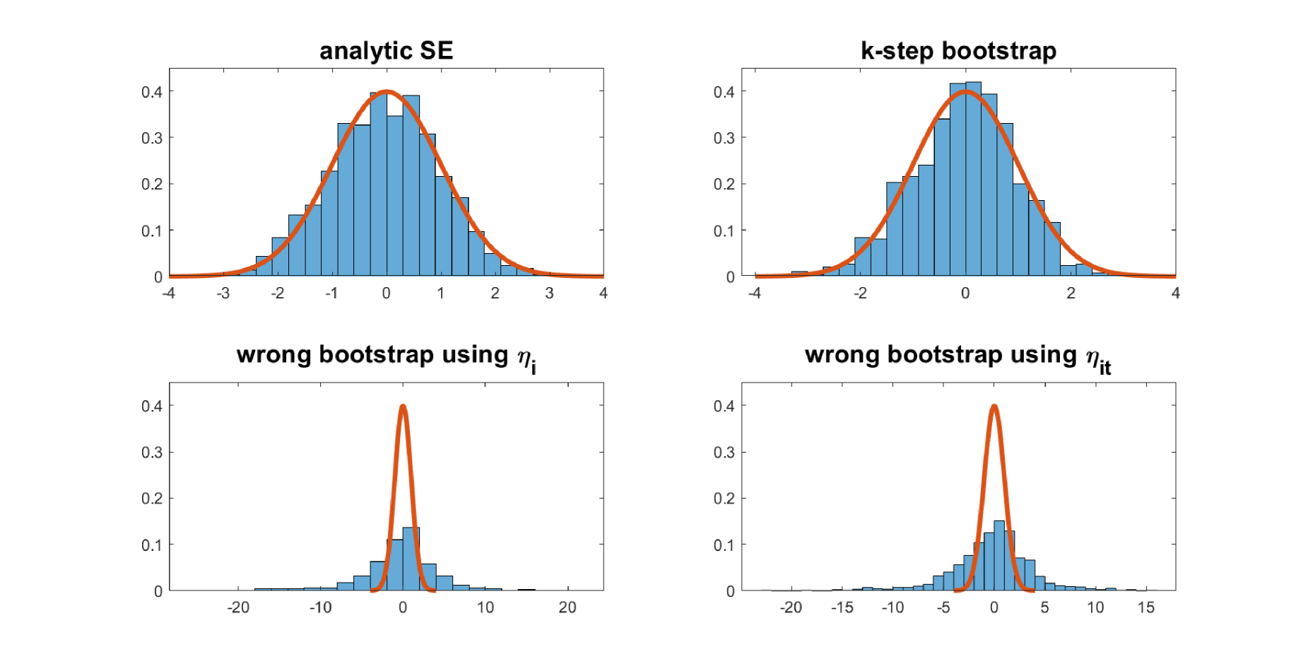
Figure 1: Histogram of t-statistics over 1000 simulation replications, and the standard normal density. The t-statistics are standardized by either the analytical standard error $\widehat{\text{SE}}(\widehat{z}_{T+1})$ (top left panel) or the bootstrap interquartile range $\sigma^{*}$ (top right panel). The bottom panels use $\eta_{i}$ and $\eta_{it}$ to generate bootstrap residuals.

To quantify the forecast uncertainty, we compute the forecast standard error of the neural network predictions, using both of the proposed methods. For method I closed-form ML, we compute the t-statistic

$$\frac{\widehat{z}_{T+1|T}-z_{T+1|T}}{\widehat{\text{SE}}(\widehat{z}_{T+1|T})},$$

where the standard error $\widehat{\text{SE}}(\widehat{z}_{T+1|T})$ has an analytical form (2.12). Here we use five Fourier bases for $\Phi(x)$. For method II “$k$-step bootstrap”, we generate the wild residual $\eta_{t}$ from the standard normal, bootstrap 100 times, and implement the $k$-step DNN bootstrap with $k=10.$ Then we compute the interquartile range of bootstrap, defined as

$$\sigma^{*}:=\frac{q^{*}_{0.75}-q^{*}_{0.25}}{z_{0.75}-z_{0.25}}$$

where $q^{*}_{\alpha}$ denotes the $\alpha$-quantile of bootstrap samples $\sum_{i}w_{i}\widehat{g}^{*,b}(x_{i,T})-\widehat{z}_{T+1|T}$, and $z_{\alpha}$ denotes the $\alpha$-quantile of the standard normal distribution. Then we also compute the t-statistic using $\sigma^{*}$ in place of $\widehat{\text{SE}}(\widehat{z}_{T+1|T})$. The interquantile range is a good proxy for the standard error obtained using bootstrap distribution, which is often used instead of the usual bootstrap standard error, because the former is guaranteed to be consistent but the latter is not.

The top two panels of Figure 1 plot the histograms of the $t$ statistics over 1000 simulations and the standard normal density function. The $t$-statistics are standardized by either $\widehat{\text{SE}}(\widehat{z}_{T+1|T})$ (left panel) or $\sigma^{*}$ (right panel). We see that although there are only 100 replications, the histograms of the t-statistics fit well to the standard normal density. Hence both proposed methods for quantifying the forecast uncertainty seem promising.

It is critical to apply the bootstrap guided by theory. In particular, the resampling must reflect the dominant source of uncertainty, namely the factor shocks from the time series. To illustrate this, we show the distribution one would obtain if the standard bootstrap were applied, i.e. the bootstrap is applied incorrectly. The bottom two panels of Figure 1 are the histograms of the bootstrap $t$-statistics (standardized by the bootstrap interquartile range), but the bootstrap residual is generated as $e_{i,t}^{*}=(y_{i,t}-\widehat{g}(x_{i,t-1}))\eta_{i}^{*}$ (the bottom left panel) and $e_{i,t}^{*}=(y_{i,t}-\widehat{g}(x_{i,t-1}))\eta_{i,t}^{*}$ (the bottom right panel), where $\eta_{i}^{*},\eta_{i,t}^{*}\sim\mathcal{N}(0,1)$. These bootstraps mistreat the forecast uncertainty as driven by the cross-sectional variation (because $\eta_{i}^{*}$ and $\eta_{i,t}^{*}$ both vary across $i$). Figure 1 clearly shows that the misuse of bootstrap vastly understates the uncertainty.

3 Applications

In this section, we outline two applications in which the confidence intervals developed for machine learning predictions can be used. The first one leads to a sparse portfolio implementation, which features a region of “non-participation” (Dow and da Costa Werlang (1992)) in portfolio allocation. In this region, the investor does not invest in a risky asset if the associated uncertainty is too large. In the second application (Section 3.2), we show how the derived FCI can be used to select asset with significantly positive expected returns via multiple hypothesis testing. In addition, in the Appendix (A.4), we also study a robust optimization approach building on Hansen and Sargent (2008).

3.1 Portfolio Selection under Uncertainty Aversion

In the first application, we apply our developed FCI to portfolio allocation. Classic portfolio theory assumes that the investor knows the population moments determining her portfolio decisions. One of the major challenges in operationalizing this theory has been that these parameters need to be estimated and that estimation errors can often dominate portfolio decisions. This issue has long been recognized, for example, the early analysis in Klein and Bawa (1976) and Michaud (1989). These shortcomings have sometimes led researchers to question whether portfolio theory can be useful for applications as pointed out in DeMiguel et al. (2009) and spurred a subsequent quest to address some of these shortcomings as in Jagannathan and Ma (2003); Kan and Zhou (2007); Tu and Zhou (2011); Yuan and Zhou (2023).

In a seminal paper, Garlappi et al. (2007) introduce a disciplined way to confront the estimation uncertainty in portfolio selection by introducing an uncertainty-averse investor. Their formulation builds on a large literature in economic theory such as Ellsberg (1961); Gilboa and Schmeidler (1989); Epstein and Wang (1994) that carefully distinguished the effects of risk vs. uncertainty aversion. In the context of portfolio selection, a risk-averse, expected utility investor behaves as if she knows the expected return and (co)variances. An uncertainty-averse investor, however, considers estimation uncertainty and integrates it into the portfolio selection problem. Implementing this approach requires the investor to be able to characterize the uncertainty, i.e. have a forecast confidence interval for the expected returns.

Chopra and Ziemba (2013) show that the effect of uncertainty in means on portfolio selection is much larger than the effect of uncertainty in variances. Our analysis therefore focuses on the effect of means. A machine learning-based estimation of covariances and their effect on portfolio selection is left for future research. Indeed, many early studies have struggled to implement mean-variance portfolio theory because means are notoriously difficult to estimate from time series. In our study, we leverage the benefits of forecasts of expected returns obtained from neural networks and also incorporate the associated estimation uncertainty. In the following, we briefly recall the main definitions of Garlappi et al. (2007).

We consider the allocation among $R$ risky assets, denoting their multivariate, conditional expected excess return as $z_{T+1|T}=(z_{1,T+1|T},...,z_{R,T+1|T})^{\prime}$ and its prediction from neural networks as $\widehat{z}_{T+1|T}=(\widehat{z}_{1,T+1|T},...,\widehat{z}_{R,T+1|T})^{\prime}$. These basis assets may be factor portfolios. In addition, we also consider the case in which the basis assets are individual asset returns. We denote the covariance matrix, $\Sigma_{T}$, which can be either for individual assets or factor portfolios. Throughout, we will denote the portfolio weights, which we aim to solve for as $\mbox{\boldmath$\omega$}=(\omega_{1},...,\omega_{R})^{\prime}$. We can now describe the portfolio selection problems.

The Markowitz (1952), i.e. standard mean-variance (MV) problem is given as:

MV problem $$\max_{\mbox{\boldmath$\omega$}}\mbox{\boldmath$\omega$}^{\prime}\widehat{z}_{T+1|T}-\frac{\gamma}{2}\mbox{\boldmath$\omega$}^{\prime}\Sigma_{T}\mbox{\boldmath$\omega$}$$ (3.1)

where $\gamma>0$ is the coefficient of risk aversion. In this problem, $\widehat{z}_{T+1|T}$ is taken as given without accounting for its associated estimation uncertainty. In contrast, the uncertainty-averse formulation explicitly considers the estimation uncertainty. It takes a “max-min” form. It can be interpreted as finding the best portfolio in the worst case for the expected return, i.e.

UA-MV problem $$\max_{\mbox{\boldmath$\omega$}}\min_{\mu\in\text{FCI}}\mbox{\boldmath$\omega$}^{\prime}\mu-\frac{\gamma}{2}\mbox{\boldmath$\omega$}^{\prime}\Sigma_{T}\mbox{\boldmath$\omega$},$$ (3.2)

where FCI is the forecast confidence interval for the expected return. The forecast confidence interval takes the following form:

$$\text{FCI}=[\widehat{z}_{1,T+1|T}-q_{1,\alpha},\widehat{z}_{1,T+1|T}+q_{1,\alpha}]\times\cdots\times[\widehat{z}_{R,T+1|T}-q_{R,\alpha},\widehat{z}_{R,T+1|T}+q_{R,\alpha}],$$

where $q_{i,\alpha}$ is the critical value for $\widehat{z}_{i,T+1|T}-z_{i,T+1}$ under significance level $\alpha$ obtained using either the analytic forecast standard error or bootstrap. For instance, using the analytic standard error, we can take

$$q_{i,\alpha}=\widehat{\operatorname{SE}}(\widehat{z}_{i,T+1|T})\times\epsilon_{\alpha},$$

where $\epsilon_{\alpha}$ corresponds to the level uncertainty aversion. If the bootstrap is used to obtain a forecast confidence interval, we can use

$$q_{i,\alpha}=q^{*}_{i,\alpha},$$

which is the $1-\alpha$ quantile of the bootstrap distribution of $\widehat{z}_{i,T+1|T}$. In applications, particularly when multiple assets are considered, controlling for the Type I error rate for multiple testing is also desirable. A simple adjustment is the Bonferroni correction, i.e. setting $\alpha=0.05/R$.

While the intuition of problem (3.2) is clear, it may appear hard to solve because of the inner maximization. Garlappi et al. (2007) characterize each element of the solution as a function of other elements. Our contribution in this framework, is in the following theorem, which shows that the UA-MV problem can be reformulated as a $\ell_{1}$- penalized optimization problem, known as Lasso.

Theorem 4.

The multivariate UA-MV problem, (3.2), is equivalent to the following adaptive Lasso formulation:

$$\min_{\mbox{\boldmath$\omega$}=(\omega_{1},...,\omega_{R})}\frac{\gamma}{2}\mbox{\boldmath$\omega$}^{\prime}\Sigma_{T}\mbox{\boldmath$\omega$}-\sum_{i=1}^{R}\omega_{i}\widehat{z}_{T+1|T,i}+\sum_{i=1}^{R}q_{\alpha,i}|\omega_{i}|.$$ (3.3)

Proof.

The proof is given in Section B.3.4. ∎

This result offers an economic justification for using penalized shrinkage portfolio selection, as developed by Ao et al. (2019) and Kozak et al. (2020). Furthermore, it justifies that the penalization parameter should be explicitly chosen as $q_{\alpha,i}$, the quantile of the ML forecast error. The following remarks provide additional guidance for implementation in different cases.

Remark 1.

If a risk-free asset is not available, $\widehat{z}_{T+1|T,i}$ denotes the raw return. Then the above problem becomes a constrained adaptive Lasso problem, i.e.

$$\min_{\mbox{\boldmath$\omega$}=(\omega_{1},...,\omega_{R})}\frac{\gamma}{2}\mbox{\boldmath$\omega$}^{\prime}\Sigma_{T}\mbox{\boldmath$\omega$}-\sum_{i=1}^{R}\omega_{i}\widehat{z}_{T+1|T,i}+\sum_{i=1}^{R}q_{\alpha,i}|\omega_{i}|,\;\;\text{subject to}\;\;\sum_{i=1}^{R}\omega_{i}=1$$

Remark 2.

The problem can be solved with standard software packages. To see this, write the Cholesky decomposition of $\Sigma_{T}$ as

$$\Sigma_{T}=LL^{\prime}$$

where $L$ is a $R\times R$ lower triangular matrix and denote $Q_{\alpha}=\text{diag}(q_{\alpha,1},...,q_{\alpha,R})$ be a diagonal matrix with elements $q_{\alpha,i}$. Then it is easy to derive that (3.2) is equivalent to the following adaptive Lasso problem:

$$\min_{\mbox{\boldmath$\omega$}}\frac{1}{2}\|Y^{*}-X^{*}\mbox{\boldmath$\omega$}\|_{2}^{2}+\|Q_{\alpha}\mbox{\boldmath$\omega$}\|_{1},\quad\text{with}\quad X^{*}=\sqrt{\gamma}L^{\prime},\;\;Y^{*}=\frac{1}{\sqrt{\gamma}}L^{-1}\widehat{z}_{T+1|T}.$$ (3.4)

If a risk-free asset is not available, the problem is again augmented with the constraint $\sum_{i=1}^{R}\omega_{i}=1$. It is well-known that the Lasso solution may be sparse and thus produce portfolio allocations, for which some (or many) $\omega_{i}$’s are zero.

The $\ell_{1}$-penalized formulation facilitates the economic interpretation of the behavior of uncertainty-averse investors compared to that of mean-variance investors. To gain the intuition, in below we study a simple case of a single risky asset:

$$\max_{\omega}\min_{\mu}\omega\mu-\frac{\gamma}{2}\omega^{2}\sigma^{2}\quad\text{subject to}\quad|\mu-\widehat{z}_{T+1|T}|\leq q_{\alpha},$$ (3.5)

where $q_{\alpha}$ denotes the $(1-\alpha)$-quantile for the predicted expected return. Corollary 5 provides a closed-form solution and allows for a comparison with the mean-variance solution in which the effect of estimation uncertainty can be seen directly. In the following, we denote $(x)_{+}=\max\{x,0\}$ and $\operatorname{sgn}(x)$ as the sign of $x$.

Corollary 5.

The uncertainty-constrained MV problem (3.5) is equivalent to the following:

$$\min_{\omega}\frac{1}{2}\left(\omega-\omega^{\operatorname{MV}}\right)^{2}+\lambda_{\alpha}|\omega|$$

and the optimal solution is

$$\omega^{\operatorname{UA}}=\operatorname{sgn}(\omega^{\operatorname{MV}})(|\omega^{\operatorname{MV}}|-\lambda_{\alpha})_{+}$$

where

$$\omega^{\operatorname{MV}}=\frac{\widehat{z}_{T+1|T}}{\gamma\sigma^{2}},\quad\lambda_{\alpha}=\frac{q_{\alpha}}{\gamma\sigma^{2}}.$$

Proof.

The proof is given in Section B.3.4. ∎

In the above theorem, $\omega^{\operatorname{MV}}$ is the classic mean-variance portfolio without uncertainty constraints, i.e. the solution to

$$\max_{\omega}\omega\widehat{z}_{T+1|T}-\frac{\gamma}{2}\omega^{2}\sigma^{2}.$$

The corollary directly illustrates why the UA-MV problem yields possible non-participation. For a fixed coefficient of risk aversion ($\gamma$) and variance ($\sigma^{2}$), an investor will choose not to invest in the risky asset if the estimation uncertainty ($q_{\alpha}$) is too large. More importantly, this result provides a direct economic interpretation of the UA-MV problem. The solution captures investor behavior in which she tests the following null hypothesis:

$$H_{0}:\quad z_{T+1|T}=0.$$

On the one hand, when she does not reject the null hypothesis, $|\widehat{z}_{T+1|T}|\leq q_{\alpha}$, the investor finds the predicted excess return not significantly different from zero as the level of uncertainty is too large. In this case, she will hold no position in the risky asset and $\omega^{\operatorname{UA}}=0$. Her optimal portfolio is then solely holding the risk-free asset. At first glance, this may seem like excessively conservative behavior. However, Bessembinder (2018) performs an extensive empirical investigation of this hypothesis and finds that many stocks do not outperform treasuries ex-post in a significant way.

On the other hand, when the investor predicts that the expected return of the risky asset is significantly different from the risk-free rate, which happens if $|\widehat{z}_{T+1|T}|>q_{\alpha}$, she then starts investing in the risky asset. The decision of whether to short or long the risky asset (the sign of $\omega^{\operatorname{UA}}$) is determined by the sign of $\widehat{z}_{T+1|T}$. However, even in this case, the investor will still invest more cautiously in the risky asset by shrinking her investment towards the risk-free rate. For instance, suppose the investor finds that $\widehat{z}_{T+1|T}>q_{\alpha}$, then her allocation in the risky asset is

$$\omega^{\operatorname{UA}}=\omega^{\operatorname{MV}}-\frac{q_{\alpha}}{\gamma\sigma^{2}}>0.$$

Instead of adopting the classic mean-variance portfolio, she reduces her allocation to the risky asset, and the amount of reduction, $q_{\alpha}/(\gamma\sigma^{2})$, reflects her tolerance towards uncertainty, which is closely linked to risk aversion.

We illustrate the optimal solution to the UA-MV problem in Figure 2. The upper panel of Figure 2 plots the optional min-max weight, $\omega^{\operatorname{UA}}$, against the classic MV portfolio. Here we fix the level of forecast standard error (FSE) and thus $q_{\alpha}$. As we can see, $\omega^{\operatorname{UA}}$ is zero for small magnitudes of $|\omega^{\operatorname{MV}}|$, i.e., the investor does not allocate towards this asset. The allocation toward the risky assets starts to increase but with constant shrinkage relative to the MVE as the latter deviates from zero. The lower panel of Figure 2 plots $\omega^{\operatorname{UA}}$ as a function of the forecast standard error for a fixed $\omega^{\operatorname{MV}}$. As the forecast standard error increases, her position in the risky asset decays linearly and eventually becomes zero.

In the case of two risky assets and no risk-free asset, we also provide an explicit solution and discuss its properties in A.3.

Figure 2: Mean-Variance vs. Uncertainty Averse (max-min) Portfolio Allocation

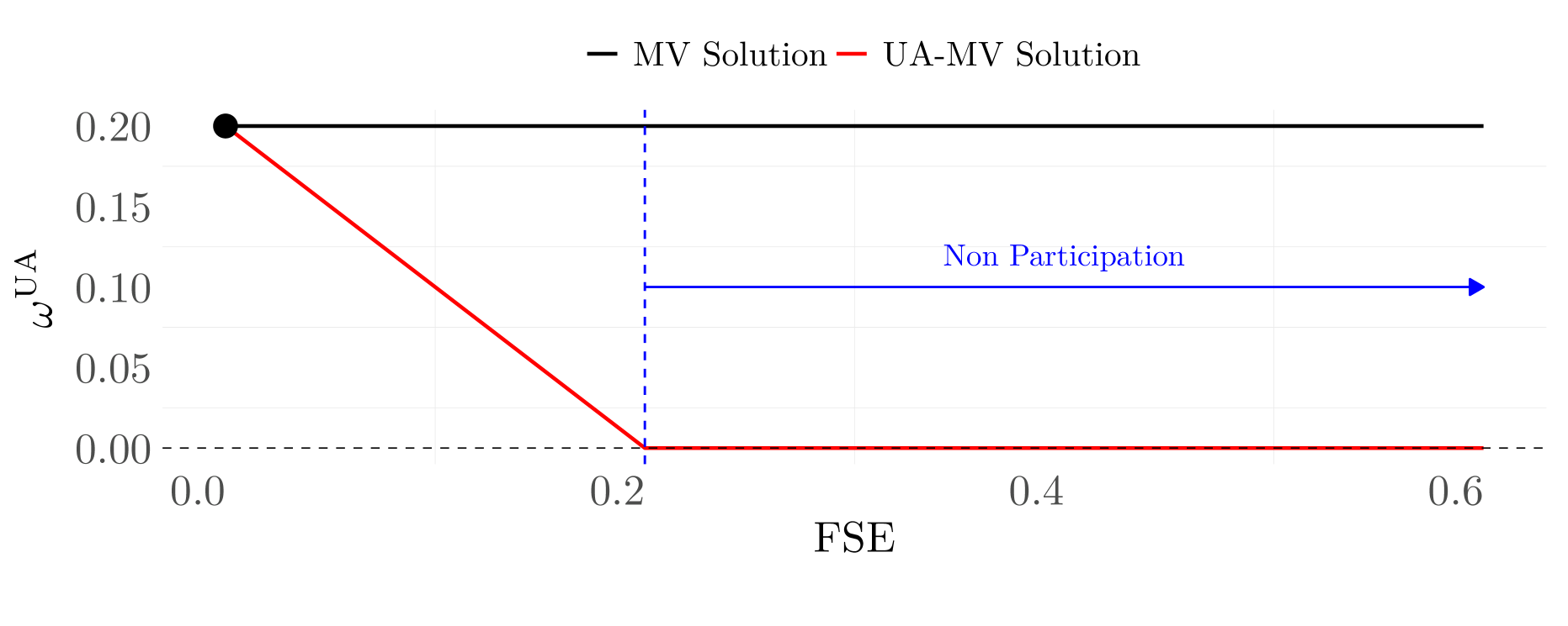
This figure shows the uncertainty averse (max-min) solution for the optimal portfolio weight in comparison with the standard mean-variance portfolio weight. In the upper panel, we hold the level of the forecast standard error (FSE) fixed and vary the mean-variance weight ($\omega^{\operatorname{MV}}$). In the lower panel, we fix the mean-variance weight at 0.2 and vary the forecast standard error (FSE).

3.2 Asset Selection

In the second application, we apply the FCI to security selection. The literature often considers long-short portfolios sorted on characteristics or return predictions typically ignoring short-sale costs. In a recent study Muravyev et al. (2024) obtain implied short-sale costs from the equity options markets and find that many anomalies are no longer profitable after accounting for short-selling fees. Moreover, several major market participants such as mutual funds are either prohibited from short-selling or do not engage in shorting for other reasons. Chen et al. (2013) document that fewer than 10% of mutual funds engage in short-selling and in general do not have large short positions. More generally, and in particular in the light of the findings of Bessembinder (2018), it is natural to ask whether expected returns are indeed significantly positive. In an intriguing analysis, he documents that the US equity premium is indeed highly concentrated and can be attributed to about 5% of stocks. While it is unlikely that our forecast confidence intervals (or any other method) can extract all ex-post winners, the use of machine learning FCI, as we describe below, highlights a good way of finding securities with positive expected returns.

In the following, we consider a long-only mutual fund manager. She needs to build a portfolio with $K$ stocks. Rather than merely allocating her funds toward the $K$ stocks with the highest predicted returns, she aims to allocate toward securities for which she has stronger conviction, i.e. those that have significantly positive predictions. So for each security under consideration, she conducts a hypothesis test

$$H_{0}^{i}:z_{i,T+1|T}=0,$$

versus the one-sided alternative

$$H_{a}^{i}:z_{i,T+1|T}>0$$

for each $i=1,...,R,$ i.e., she aims to detect which stocks have significantly and positively predicted expected returns. Given that there may be a large number of securities under consideration, this is a multiple hypotheses testing problem. Alternatively, one might consider testing if an expected excess return is significantly larger than the transaction costs associated with trading the security. We leave this extension for future research.

We compute the t-statistics of the neural network predicted excess return for each asset:

$$t_{i}=\frac{\widehat{z}_{i,T+1|T}}{\widehat{\operatorname{SE}}(\widehat{z}_{i,T+1|T})}.$$

Let $p_{i}$ denote the corresponding p-value. We then determine a cutoff value $c_{0}>0$ so that $H_{0}^{i}$ is rejected if $p_{i}<c_{0}$. The cutoff value should be determined to adjust for the type I error under the multiple testing setup. One of the widely used multiple testing adjustments is based on the false discovery rate, defined to be the expected value of $\mathcal{F}/\mathcal{R}$, where

$$\mathcal{F}=\sum_{i=1}^{N}1\{i\leq R:p_{i}<c_{0},\text{ but }z_{i,T+1|T}=0\}=\sum_{i=1}^{N}1\{H_{0}^{i}\text{ is falsely rejected}\}$$

and

$$\mathcal{R}=\sum_{i=1}^{N}1\{i\leq R:p_{i}<c_{0}\}=\sum_{i=1}^{N}1\{H_{0}^{i}\text{ is rejected}\}$$

We follow the Benjamini and Hochberg (1995) procedure, who first sort the p-values $p_{(1)}\leq\cdots\leq p_{(R)}$ and determine

$$c_{0}=p_{(K)},\quad\text{where }K=\max\{i:p_{i}\leq\alpha i/R\}$$

where $\alpha$ is the desired significance level such as 0.05. Then the false discovery rate can be controlled to be below $\alpha$, and is robust to cross-sectional dependence among tests (see Benjamini and Yekutieli (2001)).

As illustrated by Sullivan et al. (1999); Barras et al. (2010) and Harvey and Liu (2020), multiple testing is a valuable tool for mitigating data-snooping bias in performance evaluation and for selecting assets that are both statistically and economically significant. In our empirical study, we apply the outlined procedure at the individual stock level, where excess returns are predicted using neural networks. Our results demonstrate that selecting assets based on ML t-statistics, when adjusted by the forecast standard errors, delivers improved performance compared to naive selections that do not account for prediction uncertainty.

4 Empirical Analysis

4.1 Data and Implementation

We take the dataset of Jensen et al. (2022) as our starting point. It uses stock returns, volume, and price data from the Center for Research in Security prices (CRSP) monthly stock file. Our sample starts in January 1955 and ends in December 2021. The total number of stocks is slightly over 23,000 and the average number of stocks per month is approximately 3,663. Following standard conventions in the literature, we restrict the analysis to common stocks of firms incorporated in the US trading on NYSE, Nasdaq or Amex. Balance sheet data are obtained from Compustat. In order to avoid potential forward-looking biases, we lag all characteristics that are built on Compustat annually by at least six months and all that build on Compustat quarterly by at least four months. In order to mitigate a potential back-filling bias as noted by Banz and Breen (1986), we discard the first 24 months for each firm. We impute missing data using the method of Freyberger et al. (2024). Table LABEL:tab:chars_overview in the Appendix provides an overview of the 123 characteristics we employ. We obtain the 1-month T-Bill rate from Kenneth French’s data library.

Following Gu et al. (2020) we split the sample into 18 years of training (1955 - 1972), 10 years of validation (1973 - 1982) and use the remaining years (1983 - 2021) for out-of-sample testing. We re-train the model every 12 months and increase the training sample by 1 year, keeping the validation sample fixed at 10 years, but we roll it forward so that the most recent 12 months are included. For the neural network model, we use a three-layer feedforward neural network with 32, 16 and 8 neurons on the hidden layers.

After fitting the neural network, we substitute in the firm level characteristics $x_{i,T}$, and predict the individual stocks for month $T+1$ as

$$\widehat{y}_{i,T+1|T}=\widehat{g}(x_{i,T}).$$

From the previous step, we obtain predictions for each firm $i$. We then either use the predictions for individual firms in portfolio selection. We use the expected returns and their confidence intervals obtained through the machine learning models.

To compute forecast confidence intervals, we implement both the closed-form ML approximation and the $k$-step bootstrap. For the bootstrap, we set $k=10$, i.e. we re-train the models on each bootstrap sample for 10 epochs. The closed-form ML approximation uses a Fourier basis expansion $\phi(x)=(\sin(j\pi x/4),\cos(j\pi x/4),j=1...3)$. We then obtain the standard error for individual assets or portfolios following Section 2.3.1 for use in applications.

4.2 Uncertainty Averse Portfolios of Individual Stocks

We implement both the mean-variance efficient portfolio (problem (3.1)) and the uncertainty averse portfolio ((3.2)) for the 500, 750 and 1,000 largest stocks. Throughout, we use a 240-month estimation window to estimate the covariance matrix using the POET estimator (Fan et al., 2013). By conditioning on large firms with a 240 months history, we deliberately create a sample of very large firms to mitigate concerns over small and illiquid stocks. In the context of cross-sectional anomalies, Patton and Weller (2020) show that transaction cost play an important role and in the machine learning setting, Avramov et al. (2023) argue that standard implementations often concentrate the predictability on small and illiquid securities. Figure 3 plots the median effective normalized size for three scenarios, 500, 750 and 1000 largest firms with a 240-month history. The normalized size ranks the market equity of all firms each month $t$, the ranks are then divided by the number of stocks each period so that the largest firm has a normalized size of 1 and the smallest firm has a normalized size of $1/N_{t}$, where $N_{t}$ is the number of firms each period.

Figure 3: Firm Size Distribution our Sample

…

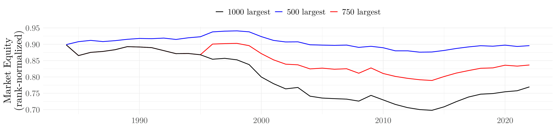
Predictions for expected returns are obtained from the neural network model. To incorporate estimation uncertainty, we can either obtain standard errors from the closed-form ML approximation, the bootstrap, or use the more conservative of the two. The latter connects well with the max-min nature of the uncertainty-averse portfolio selection approach. Table 1 shows the results for the most conservative version of the standard error. We compare the UA portfolio with three benchmarks: the mean-variance efficient portfolio (MVE), the equal-weighted portfolio (EW), and the global minimum-variance portfolio (GMVP). For the MVE, we use a coefficient of risk-aversion of one ($\gamma=1$). As we are using excess returns, there is no automatic constraint on the magnitude of the portfolio weights, we therefore normalize the standard deviation of the in-sample returns to 20% annualized for the MVE and apply this constant also to the UA portfolios; we apply a different normalizing constant for the GMVP since the weights are of different magnitude.

Table 1 shows that the MVE achieves an admirable annualized Sharpe ratio of 1.15, 1.07 and 1.16 for the three cases. This is notable since the result is achieved on a set of very large firms that are likely not subject to large liquidity frictions. It also considerably outperforms the equal-weighted portfolio and the global minimum-variance portfolio in all cases. The uncertainty-averse MV portfolio (UA 25, UA 50, and UA 75) often achieves better Sharpe ratios than the MVE. This is particularly interesting, as these portfolios are not formed to maximize the Sharpe ratio, whereas the MVE is formed to do precisely that. However, even a mean-variance investor can often achieve higher utility through the UA portfolios. The higher Sharpe ratios of the UA portfolios are achieved by reducing the standard deviation more strongly than average excess returns. Figure 4 shows the cumulative returns for the case of the 500 largest firms for the six portfolios. We can clearly see that the UA portfolios decrease less during recession periods, highlighting the mechanism of lower downside risk.

As we increase the confidence level, however, the rate of “non-participation” increases, resulting in many weights of zero as predicted by our theory. In Figure 5 we show the empirical analogue to Figure 2 for the case of the largest 500 firms. In the figure we contrast the weights of the mean-variance efficient portfolio and the UA portfolio for two dates. Clearly, we can see that the forecast uncertainty varies over time. For the example of November 1987, we set many more weights to zero in the UA portfolio, whereas we set fewer weights to zero in March 2021. In addition, we can see that the portfolio becomes more conservative as we increase the confidence level. Intuitively, the region of non-participation is proportional to the width of the confidence interval and as the confidence level increases, the region of non-participation also increases resulting in more weight of zero. Overall, the plot in Figure 2 demonstrates that the empirical results align closely with the theoretical predictions of UA-behavior outlined in Corollary 5.

Table 1: Performance Statistics for Mean-Variance and Max-Min Portfolio (conservative SE)

This table shows the annualized mean, annualized standard deviation, annualized Sharpe ratio, Sortino ratio, the maximum drawdown, the best and worst months for the mean-variance efficient portfolio (MVE), the global minimum variance portfolio (GMVP), an equal weighted portfolio and the UA-MV portfolios for the 25%, 50% and 75% confidence level. The columns Minimum Zeros, Median Zeros, Maximum Zeros show the minimum, median and maximum fraction of the portfolio weights that are set to zero in the UA-MV approach. The standard error is the maximum of the closed-form ML approximation and the bootstrap standard error using an estimation window of 240 months. All results are out-of-sample for the period from January 1983 - December 2021. Mean (%) Standard Deviation (%) Sharpe Ratio Sortino Ratio Maximum Drawdown Best Month Worst Month Minimum Zeros Median Zeros Maximum Zeros 500 largest first with 240 months history    MVE 30.37 26.32 1.15 0.57 68.49 36.26 -28.30 0.00 0.00 0.00    GMVP 23.88 31.52 0.76 0.35 74.82 39.67 -37.20 0.00 0.00 0.00    EW 10.54 15.29 0.69 0.30 53.58 14.18 -24.29 0.00 0.00 0.00    UA 25 18.89 15.94 1.19 0.60 49.09 22.79 -18.11 0.25 0.39 0.57    UA 50 10.73 8.68 1.24 0.66 27.46 11.83 -10.41 0.55 0.71 0.86    UA 75 4.73 4.28 1.11 0.59 10.97 6.58 -4.12 0.78 0.90 0.97 750 largest first with 240 months history    MVE 31.52 29.44 1.07 0.51 71.14 37.16 -38.59 0.00 0.00 0.00    GMVP 23.58 32.72 0.72 0.32 78.23 40.08 -50.49 0.00 0.00 0.00    EW 10.83 16.01 0.68 0.29 53.80 18.44 -25.72 0.00 0.00 0.00    UA 25 21.35 17.96 1.19 0.62 51.70 27.46 -23.72 0.24 0.38 0.55    UA 50 13.17 11.16 1.18 0.78 26.81 28.96 -11.68 0.53 0.70 0.87    UA 75 7.65 9.35 0.82 0.99 8.99 39.36 -4.06 0.78 0.89 0.96 1000 largest first with 240 months history    MVE 33.89 29.23 1.16 0.56 68.42 37.16 -37.57 0.00 0.00 0.00    GMVP 24.83 32.33 0.77 0.34 84.91 36.92 -45.10 0.00 0.00 0.00    EW 11.12 16.32 0.68 0.29 55.78 19.83 -25.72 0.00 0.00 0.00    UA 25 24.10 17.53 1.38 0.73 45.85 27.46 -22.22 0.25 0.37 0.55    UA 50 15.59 10.66 1.46 1.08 18.72 28.96 -10.19 0.52 0.69 0.87    UA 75 8.76 9.20 0.95 1.30 6.61 39.36 -3.22 0.76 0.89 0.96

Figure 4: Cumulative Returns for the MVE and UA Portfolio of the 500 Largest Firms

This figure shows the cumulative returns for the mean-variance efficient portfolio (MVE), the global minimum variance portfolio (GMVP), an equal-weighted portfolio, and the UA-MV portfolios for the 25%, 50%, and 75% confidence levels. The forecast uncertainty uses the conservative approach, i.e., the maximum of the analytical and bootstrap standard error. NBER recessions are depicted in gray-shaded areas. All results are out-of-sample for the period from January 1983 - December 2021.

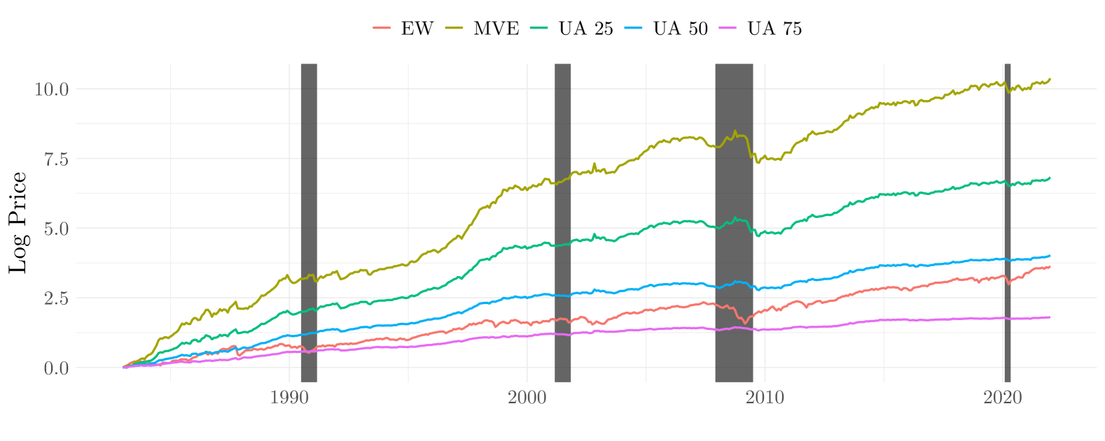
Figure 5: Portfolio Weights of the mean-variance efficient and uncertainty average portolios the 500 Largest Firms

This figure shows the weights for the mean-variance efficient portfolio (MVE) and the UA 25 (left), UA 50 (middle) and UA 75 (right) portfolio for two months (November 1987 and March 2012). The weight pairs $(\omega^{\text{MV}},\omega^{\text{UA}})$ are shown as blue dots (November 1987) and red triangles (March 2012). The weights are shown for the case of 500 largest firms with histories of 240 months.

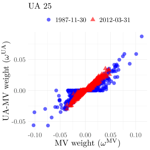
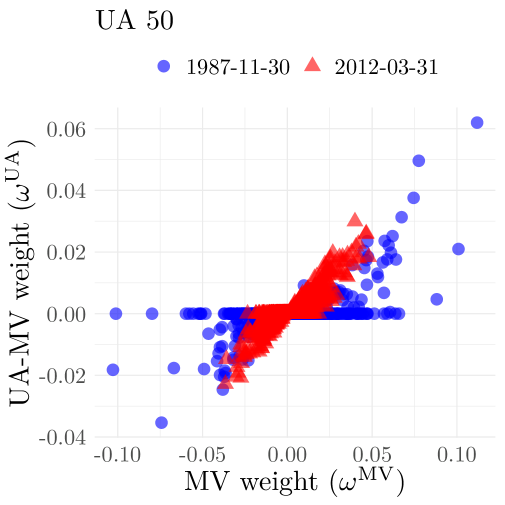
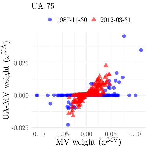
4.3 Long Only Portfolios

The classic characteristic-based anomalies are typically studied in the form of “high minus low” zero-investment portfolio. However, many large investors in the market do not engage in short-selling. Mutual funds are among the largest investors in the US equity markets and only very rarely enter into a short position. It is therefore of interest if a long-only investor could also benefit from expected returns obtained from neural networks and if the developed forecast confidence intervals are useful in their portfolio decisions. We will therefore consider a long-only mutual fund manager. The manager uses neural networks to obtain predictions for expected returns and then aims to buy the stocks with the highest predicted expected excess returns.

We will study three versions of this portfolio strategy. First, the manager conducts multiple tests:

$$H_{0}^{i}:\mathbb{E}[y_{i,T+1}|\mathcal{F}_{T}]=0,$$

versus the one-sided alternative

$$H_{a}^{i}:\mathbb{E}[y_{i,T+1}|\mathcal{F}_{T}]>0$$

for each $i=1,...,R.$ Therefore, the manager wants to focus on stocks whose expected return is significantly positive. In this setup, she uses the developed FCI to test hypotheses about the expected return predictions from neural networks. She carries out a multiple hypothesis testing adjustment using the false discovery rate as outlined in Section 3.2. The fund manager then longs the $K$ stocks with the highest predicted expected returns stocks that are also significantly positive and forms an equally weighted portfolio. We will refer to this strategy as “FCI-FDR”.

For comparison, a benchmark method is to conduct multiple tests using a $t$-test from average realized returns and their standard error, i.e.

$$t_{i}^{N}=\frac{\bar{y}_{i}}{\widehat{\operatorname{SE}}(\bar{y}_{i})},$$

where $\bar{y}_{i}$ is the average realized return and $\widehat{\operatorname{SE}}$ is the conventional standard error. We will refer to this strategy as “Naive-FDR”. Finally, consider the simplest implementation, where the fund manager simply goes long the $K$ stocks with the highest predicted expected returns using neural networks and forms an equal weighted portfolio. We will refer to this strategy as “Highest-$K$”. In our application, we will vary the size of the portfolio ($K$) between 100, 200 and 500.

It has been well documented that the features that are used in the neural network have good predictive power, and our sample necessarily covers a period during which they were particularly successful. It is therefore important to focus on relative comparisons. The upper panel of Table 2 shows the results when all firms are considered as potential investments. We see that the “Highest-$K$” portfolio achieves an annualized excess return of about 66% with a standard deviation of about 49% annually. When we compare the strategy with “Naive-FDR”, which uses realized returns to assess statistical significance, we see a non-trivial drop in average returns to 41.39% per annum. Notably, this drop is not accompanied by an equal drop in standard deviation, so that the Sharpe ratio also drops in comparison. The FCI-FDR strategy that employs the FCI for neural networks achieves an even higher average return with 67% per year with a smaller standard deviation, thus achieving the highest Sharpe ratio.

As we move from the concentrated portfolio of 100 stocks to a portfolio of 500 stocks, the average returns are lower. However, when we compare the portfolios among each other, we see the same ranking, i.e. the FCI-FDR strategy outperforms the other two in terms of risk-adjusted returns, but the magnitudes become stronger. The return difference between the FCI-FDR and the Highest-$K$ is now almost 6% per year, with a slightly lower standard deviation. The Sharpe ratio is thereby strongly improved.

In Panel B, we repeat the analysis, but only for stocks whose market capitalization is about the 25th percentile at the time of portfolio formation. This selection further mitigates liquidity concerns. Throughout panel B, we see lower average returns than in Panel A. However, the standard deviation is also lower, so that Sharpe ratios are still fairly large and often above one per year. This again confirms previous findings that the majority of cross-sectional predictability is concentrated in small firms. As we turn to the relative comparison of the three strategies, we find that the differences are now becoming more pronounced. The differences in Sharpe ratios now range between 0.2 and 0.3 per year. Interestingly, in this analysis the Naive-FDR portfolio sometimes even achieves a higher Sharpe ratio than the Highest-$K$ portfolio. Throughout the FCI-FDR portfolio achieves the highest average returns. Since FCI-FDR portfolio is not directly targeting standard deviation, it is not surprising that the standard deviations are sometimes higher than those of the other two portfolios. However, the FCI-FDR portfolio also generally displays lower drawdown, which suggests that the higher standard deviation is not due to a disproportional increase in downside risk.

In the following analysis, we compare the risk-adjusted returns of the strategies. In Table 3 we show the monthly alphas in percentage for the FCI-FDR, Highest-$K$ and the Naive-FDR strategies. We again split the analysis between using all firms and only firms above the 25th quantile of market equity. The results are consistent with and even stronger than those in Table 2. The difference in alphas between the FCI-FDR and the Highest-$K$ (and the Naive-FDR) is larger than the return spreads. It is noteworthy that often the alphas get larger when we add the momentum factor. For example, when we move from the Fama and French (1993) three-factor model (FF3) to the FF4 (FF3 + momentum) model, the alpha increases. This happens because many of these portfolios have negative exposure to the momentum factor, which in turn has a positive risk premium. For the case of all firms (Panel A), we see that the difference in alpha between the FCI-FDR portfolio and the Highest-$K$ is of the same magnitude as the difference in returns.

For the case of the larger firms in Panel B of Table 3, we see that the level of alphas is lower than in the upper panel. However, many alphas are larger than 1% per month and still strongly significant – all alphas in Table 3 pass the $t$-stat 3 hurdle proposed by Harvey et al. (2016). In all cases, the FCI-FDR strategy achieves higher alphas than the highest-$K$ strategy. The difference is more pronounced for larger portfolios. The results therefore underscore the importance of accounting for forecast uncertainties in constructing portfolios.

Table 2: Performance Statistics for Best $K$ Portfolio (conservative SE)

This table shows the annualized mean, annualized standard deviation, annualized Sharpe ratio, Sortino ratio, the maximum drawdown, the best and worst months for the following portfolio: “FCI-FDR” is the portfolio that longs the $K$ stocks with the highest predicted expected excess returns that are significantly greater than zero. The “Highest-$K$” portfolio is to long the $K$ largest predicted returns. The “Naive-FDR” is the portfolio of the $K$ largest predicted returns for which the average realized returns are significantly greater than zero. In all cases we use the False Discovery Rate (FDR) as a multiple testing adjustment, as outlined in Section 3.2. We vary the size of the portfolio between 100, 200 and 500. The upper panel of the table shows the results when all stocks are potential candidates for the portfolios. The lower panel considers stocks whose market capitalization is larger than the 25% quantile of firms’ market capitalization at the time of portfolio formation. The standard error used in FCI-FDR is the maximum of the closed-form ML approximation and the bootstrap standard error using an estimation window of 240 months. The portfolios are equal weighted and all results are out-of-sample for the period from January 1983 - December 2021. # Stocks ($K$) Mean (%) Standard Deviation (%) Sharpe Ratio Sortino Ratio Maximum Drawdown Best Month Worst Month Panel A: All Firms    FCI-FDR 100 67.33 44.48 1.51 1.30 52.16 100.70 -26.44    Highest-$K$ 100 66.98 48.80 1.37 1.13 55.54 100.66 -28.28    Naive-FDR 100 41.39 36.13 1.15 0.77 60.24 89.25 -30.44    FCI-FDR 200 55.19 37.98 1.45 1.23 49.71 96.61 -26.31    Highest-$K$ 200 52.67 42.25 1.25 0.95 58.04 96.08 -29.48    Naive-FDR 200 33.28 29.36 1.13 0.68 57.26 74.03 -30.04    FCI-FDR 500 44.05 31.46 1.40 1.10 42.91 81.51 -26.16    Highest-$K$ 500 38.52 33.01 1.17 0.78 57.00 85.35 -28.42    Naive-FDR 500 25.79 22.67 1.14 0.60 52.18 46.27 -27.76 Panel B: Firm greater than 25% market equity    FCI-FDR 100 29.16 26.69 1.09 0.64 50.07 65.14 -29.18    Highest-$K$ 100 26.91 33.18 0.81 0.45 62.11 75.89 -35.82    Naive-FDR 100 23.89 25.94 0.92 0.46 57.19 51.80 -31.60    FCI-FDR 200 27.16 24.10 1.13 0.62 48.51 41.15 -28.83    Highest-$K$ 200 23.71 27.73 0.85 0.45 60.37 58.67 -34.36    Naive-FDR 200 21.65 22.54 0.96 0.46 54.93 36.25 -29.61    FCI-FDR 500 25.20 23.00 1.10 0.58 47.26 41.15 -28.83    Highest-$K$ 500 20.79 22.34 0.93 0.45 56.22 35.76 -29.08    Naive-FDR 500 19.28 19.79 0.97 0.45 51.01 21.46 -27.50

Table 3: Alpha for Best $K$ Portfolio (conservative SE)

This table shows monthly alphas in percentage of regression of the excess returns of the three strategies onto risk factors. CAPM represents the CAPM, FF3 refers to the Fama and French (1993) three-factor model, FF4 denotes the FF3 model, augmented with the momentum factor (Carhart (1997)), FF5 is the Fama and French (2016), FF6 adds the momentum factor to the five-factor model, FF6+ adds the short-term reversal factor. All data are obtained from Kenneth French’s data library. “FCI-FDR” is the portfolio that longs the $K$ stocks with the highest predicted expected returns that are significantly greater than zero. The “Highest-$K$” longs the $K$ largest predicted returns. The “Naive-FDR” is the portfolio of the $K$ largest predicted returns for which the average realized returns are significantly greater than zero. In all cases we use the False Discovery Rate (FDR) as a multiple testing adjustment. The procedure is outlined in Section 3.2. We vary the size of the portfolio between 100, 200 and 500. The upper panel of the table shows the results when all stocks are potential candidates for the portfolios. The lower panel only considers stocks whose market capitalization is larger than the 25% quantile of firms’ market capitalization at the time of portfolio formation. The standard error used in FCI-FDR is the maximum of the closed-form ML approximation and the bootstrap standard error using an estimation window of 240 months. The portfolios are equally weighted and all results are out-of-sample for the period from January 1983 - December 2021.

	# Stocks ($K$)	CAPM	FF3	FF4	FF5	FF6	FF6+
All Firms
FCI-FDR	100	4.53***	4.61***	5.24***	5.11***	5.58***	5.38***
Highest-$K$	100	4.37***	4.48***	5.20***	5.04***	5.57***	5.37***
Naive-FDR	100	2.40***	2.44***	2.93***	2.76***	3.13***	2.94***
FCI-FDR	200	3.62***	3.65***	4.23***	4.00***	4.43***	4.27***
Highest-$K$	200	3.25***	3.33***	3.98***	3.76***	4.24***	4.05***
Naive-FDR	200	1.81***	1.83***	2.21***	2.07***	2.35***	2.20***
FCI-FDR	500	2.76***	2.75***	3.24***	2.95***	3.32***	3.19***
Highest-$K$	500	2.21***	2.24***	2.73***	2.56***	2.93***	2.77***
Naive-FDR	500	1.28***	1.26***	1.45***	1.34***	1.48***	1.38***
Firm greater than 25% market equity
FCI-FDR	100	1.55***	1.48***	1.81***	1.50***	1.75***	1.62***
Highest-$K$	100	1.09***	1.09***	1.62***	1.37***	1.76***	1.59***
Naive-FDR	100	0.98***	0.97***	1.22***	1.08***	1.26***	1.14***
FCI-FDR	200	1.41***	1.33***	1.58***	1.28***	1.47***	1.36***
Highest-$K$	200	0.93***	0.91***	1.27***	1.05***	1.33***	1.19***
Naive-FDR	200	0.87***	0.83***	0.98***	0.86***	0.97***	0.88***
FCI-FDR	500	1.26***	1.17***	1.39***	1.10***	1.27***	1.17***
Highest-$K$	500	0.81***	0.76***	0.95***	0.78***	0.93***	0.83***
Naive-FDR	500	0.75***	0.70***	0.76***	0.65***	0.70***	0.63***

5 Conclusion

The asset pricing literature has long recognized that machine learning uncertainty should be explicitly considered in making portfolio decisions. The framework of uncertainty aversion provides a disciplined way to incorporate such uncertainty about input parameters. This however requires a (asymptotic) distribution theory of the parameters. Although machine learning methods have shown great progress in forecasting expected returns, considering their estimation uncertainty in portfolio choice has remained an open problem due to a lack of distribution theory.

We introduce new methods to quantify prediction uncertainty in machine learning forecasts of asset returns. We show that neural network forecasts of expected returns share the same asymptotic distribution as classic nonparametric methods such as Fourier series, enabling a closed-form expression for their standard errors. We also propose a $k$-step bootstrap that simulates the asymptotic distribution without repeatedly retraining networks, thus dramatically reducing computational costs. We then incorporate these forecast confidence intervals into an uncertainty-averse investment framework. This leads to “non-participation” in assets when uncertainty exceeds a threshold, providing an economic rationale for shrinkage for portfolio selection. Empirically, our methods improve out-of-sample performance while mitigating multiple testing problems.

We have illustrated two areas of application; the distribution theory is general and can be used in other applications. An interesting analysis might be to consider “real-time” machine learning in cross-sectional asset pricing as in Li et al. (2024) to examine pre- vs.  post publication effects. We leave this application for future research.

Appendix A Additional Results

A.1 Figures and Tables

Table 4: Overview of the Characteristics

This table gives an overview of the characteristic used in the empirical analysis. They are obtained from Jensen et al. (2022). We refer to their paper and the companion website for the precise construction and reference to the original paper that proposed these predictors.
Acronym	Description	Category	In-Sample
age	Firm age	Intangibles	1965 - 2001
aliq_at	Liquidity of book assets	Intangibles	1984 - 2006
aliq_mat	Liquidity of market assets	Intangibles	1984 - 2006
cash_at	Cash-to-assets	Intangibles	1972 - 2009
dgp_dsale	Change gross margin minus change sales	Intangibles	1974 - 1988
dsale_dinv	Change sales minus change Inventory	Intangibles	1974 - 1988
dsale_drec	Change sales minus change receivables	Intangibles	1974 - 1988
kz_index	Kaplan-Zingales index	Intangibles	1968-1995
opex_at	Operating leverage	Intangibles	1963 - 2008
sale_emp_gr1	Labor force efficiency	Intangibles	1974 - 1988
seas_11_15an	Years 11-15 lagged returns, annual	Intangibles	1965 - 2002
seas_11_15na	Years 11-15 lagged returns, nonannual	Intangibles	1965 - 2002
seas_16_20an	Years 16-20 lagged returns, annual	Intangibles	1965 - 2002
seas_16_20na	Years 16-20 lagged returns, nonannual	Intangibles	1965 - 2002
seas_1_1an	Year 1-lagged return, annual	Intangibles	1965 - 2002
seas_1_1na	Year 1-lagged return, nonannual	Intangibles	1965 - 2002
seas_2_5an	Years 2-5 lagged returns, annual	Intangibles	1965 - 2002
seas_2_5na	Years 2-5 lagged returns, nonannual	Intangibles	1965 - 2002
seas_6_10an	Years 6-10 lagged returns, annual	Intangibles	1965 - 2002
seas_6_10na	Years 6-10 lagged returns, nonannual	Intangibles	1965 - 2002
tangibility	Asset tangibility	Intangibles	1973-2001
at_gr1	Asset Growth	Investment	1968 - 2003
be_gr1a	Change in common equity	Investment	1962 - 2001
capex_abn	Abnormal corporate investment	Investment	1973 - 1996
capx_gr1	CAPEX growth (1 year)	Investment	1971-1992
capx_gr2	CAPEX growth (2 years)	Investment	1976 - 1998
capx_gr3	CAPEX growth (3 years)	Investment	1976 - 1998
chcsho_12m	Net stock issues	Investment	1970 - 2003
coa_gr1a	Change in current operating assets	Investment	1962 - 2001
col_gr1a	Change in current operating liabilities	Investment	1962 - 2001
cowc_gr1a	Change in current operating working capital	Investment	1962 - 2001
dbnetis_at	Net debt issuance	Investment	1971 - 2000
eqnpo_12m	Equity net payout	Investment	1968 - 2003
fnl_gr1a	Change in financial liabilities	Investment	1962 - 2001
inv_gr1	Inventory growth	Investment	1965 - 2009
inv_gr1a	Inventory change	Investment	1970 - 1997
ncoa_gr1a	Change in noncurrent operating assets	Investment	1962 - 2001
ncol_gr1a	Change in noncurrent operating liabilities	Investment	1962 - 2001
nfna_gr1a	Change in net financial assets	Investment	1962 - 2001
nncoa_gr1a	Change in net noncurrent operating assets	Investment	1962 - 2001
noa_at	Net operating assets	Investment	1964-2002
noa_gr1a	Change in net operating assets	Investment	1964-2002
oaccruals_at	Operating accruals	Investment	1962 - 1991
oaccruals_ni	Percent operating accruals	Investment	1989 - 2008
ppeinv_gr1a	Change PPE and Inventory	Investment	1970 - 2005
taccruals_at	Total accruals	Investment	1962 - 2001
taccruals_ni	Percent total accruals	Investment	1989 - 2008
prc_highprc_252d	Current price to high price over last year	Momentum	1963 - 2001
resff3_12_1	Residual momentum t-12 to t-1	Momentum	1930 - 2009
resff3_6_1	Residual momentum t-6 to t-1	Momentum	1930 - 2009
ret_12_1	Price momentum t-12 to t-1	Momentum	1965 - 1989
ret_6_1	Price momentum t-6 to t-1	Momentum	1965 - 1989
tax_gr1a	Tax expense surprise	Momentum	1977 - 2006
corr_1260d	Market correlation	New	1925 - 2015
mispricing_mgmt	Mispricing factor: Management	New	1967 - 2013
mispricing_perf	Mispricing factor: Performance	New	1967 - 2013
ni_be	Return on equity	New	1979 - 1993
ocf_at	Operating cash flow to assets	New	1990 - 2015
ocf_at_chg1	Change in operating cash flow to assets	New	1990 - 2015
qmj_prof	Quality minus Junk: Profitability	New	1957 - 2016
qmj_safety	Quality minus Junk: Safety	New	1957 - 2016
ret_12_7	Price momentum t-12 to t-7	New	1925 - 2010
ret_3_1	Price momentum t-3 to t-1	New	1965 - 1989
ret_9_1	Price momentum t-9 to t-1	New	1965 - 1989
rmax5_21d	Highest 5 days of return	New	1993 - 2012
rmax5_rvol_21d	Highest 5 days of return scaled by volatility	New	1925-2015
at_be	Book leverage	Profitability	1963 - 1990
at_turnover	Capital turnover	Profitability	1979 - 1993
cop_at	Cash-based operating profits-to-book assets	Profitability	1967 - 2016
cop_atl1	Cash-based operating profits-to-lagged book assets	Profitability	1963 - 2014
ebit_bev	Return on net operating assets	Profitability	1984 - 2002
ebit_sale	Profit margin	Profitability	1984 - 2002
f_score	Pitroski F-score	Profitability	1976 - 1996
gp_at	Gross profits-to-assets	Profitability	1963 - 2010
gp_atl1	Gross profits-to-lagged assets	Profitability	1967 - 2016
o_score	Ohlson O-score	Profitability	1981 - 1995
op_at	Operating profits-to-book assets	Profitability	1963 - 2013
op_atl1	Operating profits-to-lagged book assets	Profitability	1963 - 2014
ope_be	Operating profits-to-book equity	Profitability	1963 - 2013
ope_bel1	Operating profits-to-lagged book equity	Profitability	1967 - 2016
pi_nix	Taxable income-to-book income	Profitability	1973-2000
sale_bev	Asset turnover	Profitability	1984 - 2002
ami_126d	Amihud Measure	Trading Frictions	1964 - 1997
beta_60m	Market Beta	Trading Frictions	1935 - 1968
beta_dimson_21d	Dimson beta	Trading Frictions	1955 - 1974
betabab_1260d	Frazzini-Pedersen market beta	Trading Frictions	1926 - 2012
betadown_252d	Downside beta	Trading Frictions	1963 - 2001
bidaskhl_21d	The high-low bid-ask spread	Trading Frictions	1927 - 2006
coskew_21d	Coskewness	Trading Frictions	1963 - 1993
dolvol_126d	Dollar trading volume	Trading Frictions	1966 - 1995
dolvol_var_126d	Coefficient of variation for dollar trading volume	Trading Frictions	1966 - 1995
iskew_capm_21d	Idiosyncratic skewness from the CAPM	Trading Frictions	1967 - 2016
iskew_ff3_21d	Idiosyncratic skewness from the Fama-French 3-factor model	Trading Frictions	1925-2012
ivol_capm_21d	Idiosyncratic volatility from the CAPM (21 days)	Trading Frictions	1967 - 2016
ivol_capm_252d	Idiosyncratic volatility from the CAPM (252 days)	Trading Frictions	1976 - 1997
ivol_ff3_21d	Idiosyncratic volatility from the Fama-French 3-factor model	Trading Frictions	1963 - 2000
market_equity	Market Equity	Trading Frictions	1926 - 1975
prc	Price per share	Trading Frictions	1940 - 1978
ret_1_0	Short-term reversal	Trading Frictions	1929 - 1982
rmax1_21d	Maximum daily return	Trading Frictions	1962 -2005
rskew_21d	Total skewness	Trading Frictions	1925-2012
rvol_21d	Return volatility	Trading Frictions	1963 - 2000
turnover_126d	Share turnover	Trading Frictions	1963 - 1991
turnover_var_126d	Coefficient of variation for share turnover	Trading Frictions	1966 - 1995
zero_trades_126d	Number of zero trades with turnover as tiebreaker (6 months)	Trading Frictions	1963 - 2003
zero_trades_21d	Number of zero trades with turnover as tiebreaker (1 month)	Trading Frictions	1963 - 2003
zero_trades_252d	Number of zero trades with turnover as tiebreaker (12 months)	Trading Frictions	1963 - 2003
at_me	Assets-to-market	Value	1963 - 1990
be_me	Book-to-market equity	Value	1973 - 1984
bev_mev	Book-to-market enterprise value	Value	1962 - 2001
debt_me	Debt-to-market	Value	1948 - 1979
div12m_me	Dividend yield	Value	1940 -1980
ebitda_mev	Ebitda-to-market enterprise value	Value	1963 - 2009
eq_dur	Equity duration	Value	1962 - 1998
fcf_me	Free cash flow-to-price	Value	1963 - 1990
ival_me	Intrinsic value-to-market	Value	1975 - 1993
netdebt_me	Net debt-to-price	Value	1962 - 2001
ni_me	Earnings-to-price	Value	1963-1979
ocf_me	Operating cash flow-to-market	Value	1973 - 1997
ret_60_12	Long-term reversal	Value	1926 - 1982
sale_gr1	Sales Growth (1 year)	Value	1968 - 1989
sale_gr3	Sales Growth (3 years)	Value	1968 - 1989
sale_me	Sales-to-market	Value	1979-1991

Table 5: Performance Statistics for Mean-Variance and Max-Min Portfolio (analytical SE)

This table shows the annualized mean, annualized standard deviation, annualized Sharpe ratio, Sortino ratio, the maximum drawdown, the best and worst months for the mean-variance efficient portfolio (MVE), the global minimum variance portfolio (GMVP), an equal-weighted portfolio and the UA-MV portfolios for the 25%, 50% and 75% confidence level. The standard error is obtained from the closed-form ML approximation using an estimation window of 240 months. All results are out-of-sample for the period from January 1983 - December 2021. Mean (%) Standard Deviation (%) Sharpe Ratio Sortino Ratio Maximum Drawdown Best Month Worst Month 500 largest first with 240 months history    MVE 30.37 26.32 1.15 0.57 68.49 36.26 -28.30    GMVP 23.88 31.52 0.76 0.35 74.82 39.67 -37.20    EW 10.54 15.29 0.69 0.30 53.58 14.18 -24.29    UA 25 19.12 16.38 1.17 0.58 49.87 23.38 -18.11    UA 50 11.21 9.21 1.22 0.65 28.02 13.02 -10.41    UA 75 5.07 4.78 1.06 0.56 11.76 8.03 -4.58 750 largest first with 240 months history    MVE 31.52 29.44 1.07 0.51 71.14 37.16 -38.59    GMVP 23.58 32.72 0.72 0.32 78.23 40.08 -50.49    EW 10.83 16.01 0.68 0.29 53.80 18.44 -25.72    UA 25 20.84 18.70 1.11 0.57 51.51 31.54 -23.86    UA 50 12.36 11.56 1.07 0.65 29.57 34.20 -11.20    UA 75 6.73 8.39 0.80 0.75 14.13 39.80 -4.17 1000 largest first with 240 months history    MVE 33.89 29.23 1.16 0.56 68.42 37.16 -37.57    GMVP 24.83 32.33 0.77 0.34 84.91 36.92 -45.10    EW 11.12 16.32 0.68 0.29 55.78 19.83 -25.72    UA 25 23.48 18.26 1.29 0.67 45.24 31.54 -23.86    UA 50 14.64 11.09 1.32 0.87 29.57 34.20 -11.20    UA 75 7.70 8.24 0.93 0.90 14.13 39.80 -4.40

Table 6: Performance Statistics for Mean-Variance and Max-Min Portfolio (bootstrap SE)

This table shows the annualized mean, annualized standard deviation, annualized Sharpe ratio, Sortino ratio, the maximum drawdown, the best and worst months for the mean-variance efficient portfolio (MVE), the global minimum variance portfolio (GMVP), an equal-weighted portfolio and the UA-MV portfolios for the 25%, 50% and 75% confidence level. The standard error is obtained from the $k$-step bootstrap. All results are out-of-sample for the period from January 1983 - December 2021. Mean (%) Standard Deviation (%) Sharpe Ratio Sortino Ratio Maximum Drawdown Best Month Worst Month 500 largest first with 240 months history    MVE 30.37 26.32 1.15 0.57 68.49 36.26 -28.30    GMVP 23.88 31.52 0.76 0.35 74.82 39.67 -37.20    EW 10.54 15.29 0.69 0.30 53.58 14.18 -24.29    UA 25 21.73 18.84 1.15 0.56 56.70 25.60 -22.33    UA 50 14.36 13.11 1.10 0.53 43.21 15.36 -16.72    UA 75 8.36 8.21 1.02 0.51 27.99 9.44 -10.40 750 largest first with 240 months history    MVE 31.52 29.44 1.07 0.51 71.14 37.16 -38.59    GMVP 23.58 32.72 0.72 0.32 78.23 40.08 -50.49    EW 10.83 16.01 0.68 0.29 53.80 18.44 -25.72    UA 25 23.78 20.85 1.14 0.56 61.43 27.37 -31.66    UA 50 16.73 15.20 1.10 0.57 49.40 28.34 -22.69    UA 75 10.96 11.80 0.93 0.62 31.12 40.69 -14.47 1000 largest first with 240 months history    MVE 33.89 29.23 1.16 0.56 68.42 37.16 -37.57    GMVP 24.83 32.33 0.77 0.34 84.91 36.92 -45.10    EW 11.12 16.32 0.68 0.29 55.78 19.83 -25.72    UA 25 26.40 20.33 1.30 0.64 58.38 27.37 -31.48    UA 50 19.39 14.51 1.34 0.71 46.44 28.34 -21.86    UA 75 13.05 11.34 1.15 0.82 29.40 40.69 -14.57

A.2 Tuning Parameters

Table 7 summarizes the tuning parameters for the three-layer feedforward neural network. For the Fourier series regressions we set the Fourier basis functions as $(\sin(j\pi x/4),\cos(j\pi x/4))$ for $j=1,...,J$.

Table 7: Tuning Parameters for the Neural Network and Fourier Basis

Parameter	Values
L2 Penalty	$\lambda_{2}\in\{1e^{-5},1e^{-3}\}$
Learning Rate	$\eta=0.001$
Batch Size	10,000
Epochs	100
Activation Function	ReLu
Algorithm	Adam (default parameters)
Num. Fourier Basis	$J=3$

A.3 The UA-MV Portfolio without Risk-free Rate

We now consider the problem where the investor would like to allocate her portfolio into $R$ risky assets without risk-free rate. Then $z_{T+1|T,i}$ for $i=1,...,R$ denote the expected returns. To incorporate her uncertainty constraints for forecasting the expected returns, the investor then formulates a multivariate, constrained, mean-variance problem:

$$\max_{\mbox{\boldmath$\omega$}=(\omega_{1},...,\omega_{R})}\min_{\mu_{1},...,\mu_{R}}\sum_{i=1}^{R}\omega_{i}\mu_{i}-\frac{\gamma}{2}\mbox{\boldmath$\omega$}^{\prime}\Sigma_{T}\mbox{\boldmath$\omega$}$$

subject to the constraint on $(\mbox{\boldmath$\omega$},\mu_{1},...,\mu_{R})$:

$$\sum_{j=1}^{R}\omega_{j}=1,\quad|\mu_{i}-\widehat{z}_{T+1|T,i}|\leq q_{\alpha,i},i=1,...,R.$$

To see how the investor’s uncertainty aversion determines the portfolio shrinkage, we focus on the case when there are two risky assets ($R=2$), as this allows us to gain the most intuition. Since the expressions of the optimal portfolios $\omega_{1}^{*}$ and $\omega_{2}^{*}$ are symmetric, we will focus on $\omega_{1}^{*}$. The optimal portfolio has a closed-form solution: for $c_{0}=\gamma^{-1}\operatorname{Var}(z_{T+1,1}-z_{T+1,2})^{-1}$ (see Section B.4 for the proof).

$$\omega_{1}^{*}=\begin{cases}0&\text{when }-c_{0}(q_{\alpha,1}+q_{\alpha,2})<\omega_{1}^{\operatorname{MV}}<c_{0}(q_{\alpha,k}-q_{\alpha,j})\cr\omega_{1}^{\operatorname{MV}}+c_{0}(q_{\alpha,1}+q_{\alpha,2})&\text{when }\omega_{1}^{\operatorname{MV}}<-c_{0}(q_{\alpha,1}+q_{\alpha,2})\cr\omega_{1}^{\operatorname{MV}}-c_{0}(q_{\alpha,k}-q_{\alpha,j})&\text{when }\omega_{1}^{\operatorname{MV}}>c_{0}(q_{\alpha,1}-q_{\alpha,2})\text{ and }\omega_{2}^{\operatorname{MV}}>c_{0}(q_{\alpha,2}-q_{\alpha,1})\end{cases}.$$ (A.1)

Here $\omega_{1}^{\operatorname{MV}}$ is the usual mean-variance efficient portfolio: $\omega_{2}^{\operatorname{MV}}=1-\omega_{1}^{\operatorname{MV}}$ and

$$\omega_{1}^{\operatorname{MV}} := \arg\max_{\omega\in\mathbb{R}}\omega\widehat{z}_{T+1|T,1}+(1-\omega)\widehat{z}_{T+1|T,2}-\frac{\gamma}{2}\mbox{\boldmath$\omega$}^{\prime}\Sigma_{T}\mbox{\boldmath$\omega$},\quad\mbox{\boldmath$\omega$}=(\omega,1-\omega)^{\prime}.$$

There are three cases, the investor holds no position in the first asset, the investor holds a short-position in the first asset and the investors invests a positive amount in the first asset. To explain the economic intuition, let us compare the behavior of two investors: one MV-investor, who adopts $\omega_{1}^{\operatorname{MV}}$; and one UA-investor, who is uncertainty averse and adopts $\omega_{1}^{*}$.

Consider the first case of (A.1). The “non-participation” position $\omega_{1}^{*}=0$ appears when

$$|\omega_{1}^{\operatorname{MV}}+q_{\alpha,2}c_{0}|\leq q_{\alpha,1}c_{0}.$$ (A.2)

Recall that $q_{\alpha,k}$ measures the UA-investor’s degree of uncertainty aversion. The higher $q_{\alpha,k}$, the more cautious she is when allocating to asset $k$, and vice versa. Suppose $q_{\alpha,2}\to 0$ and is much smaller than $q_{\alpha,1}$. When (A.2) holds, then

$$|\omega_{1}^{\operatorname{MV}}|\leq q_{\alpha,1}c_{0}[1+o(1)],$$

meaning that the MV-investor will not invest in $z_{T+1,1}$ more than $q_{\alpha,1}c_{0}$. Meanwhile, as $q_{\alpha,2}$ is very small, the UA-investor has little uncertainty about the predictor $\widehat{z}_{T+1|T,2}$, so she is be better off by allocating all her assets in $z_{T+1,2}$, and thus $\omega_{1}^{*}=0$.

Next, consider the second case in (A.1). In this case $\omega_{1}^{\operatorname{MV}}<0$, meaning that the MV-investor will short the first asset. Meanwhile, the UA-investor will also short asset 1 because $\omega_{1}^{*}=\omega_{1}^{\operatorname{MV}}+c_{0}(q_{\alpha,1}+q_{\alpha,2})<0$. However, she will short less of asset 1 and shift her allocation towards asset 2, as $\omega_{1}^{\operatorname{MV}}<\omega_{1}^{*}<0$. The amount of shrinkage is $c_{0}(q_{\alpha,1}+q_{\alpha,2})$. Therefore, the UA-investor is more cautious than the MV-investor when shorting.

Finally, consider the third case of (A.1), then

$$\omega_{1}^{*}=\omega_{1}^{\operatorname{MV}}-c_{0}(q_{\alpha,1}-q_{\alpha,2}),\text{ which is }\begin{cases}<\omega_{1}^{\operatorname{MV}}&\text{ if }q_{\alpha,1}>q_{\alpha,2}\cr>\omega_{1}^{\operatorname{MV}}&\text{ if }q_{\alpha,1}<q_{\alpha,2}.\end{cases}$$

When $q_{\alpha,1}>q_{\alpha,2}$, this case implies $\omega_{1}^{\operatorname{MV}}>c_{0}(q_{\alpha,1}-q_{\alpha,2})>0$, so the MV-investor will have a long position in asset 1. Meanwhile, because the UA-investor is more uncertain about $z_{T+1,1}$ than $z_{T+1,2}$, her allocation in the first asset satisfies $0<\omega_{1}^{*}<\omega_{1}^{\operatorname{MV}}$, meaning that she shrinks her allocation toward the second asset. The amount of shrinkage, $c_{0}(q_{\alpha,1}-q_{\alpha,2})$, is proportional to the difference in the degrees of uncertainty. The case when $q_{\alpha,1}<q_{\alpha,2}$ follows from a similar insight due to the symmetry between $\omega_{1}^{*}$ and $\omega_{2}^{*}$.

A.4 Risk-Sensitive Optimization

The UA-constrained portfolio allocation tends to adopt a non-participation, which may be overly conservative. In this subsection, we introduce a less restrictive framework that explicitly accounts for forecast uncertainty. Our approach builds on the robust decision-making framework of Hansen and Sargent (2008).

A.4.1 One risky and one risk-free asset

Anderson and Cheng (2016) formulate a mean-variance optimization for choosing portfolio allocations that are robust to misspecification in the predictive model. To illustrate, consider an example with one risky asset with excess return $z_{T+1}$. Their problem is formulated as:

$$\max_{\omega}\min_{h_{T}}\omega\mathbb{E}_{h_{T}}(z_{T+1})-\frac{\gamma}{2}\omega^{2}\operatorname{Var}_{h_{T}}(z_{T+1})+\frac{1}{\tau}D(h_{T}||f_{T})$$ (A.3)

where both $h_{T}$ and $f_{T}$ are probability density functions, and $\mathbb{E}_{h_{T}}(z_{T+1})$ and $\operatorname{Var}_{h_{T}}(z_{T+1})$ respectively denote the expectation and variance of the future risky return with respect to the distribution $h_{T}$; $D(h_{T}||f_{T})$ denotes the Kulback-Leibler divergence from $f_{T}$ to $h_{T}$. Therefore, different from the UA-constrained problem, (A.3) introduces an inner optimization with respect to the density function $h_{T}$ with an additional measure $D(h_{T}||f_{T})$. This problem is also called “risk-sensitive optimization” by Hansen and Sargent (2008).

The idea is that the investor takes $f_{T}$ as the benchmark predictive density of $z_{T+1}$, but she is concerned that $f_{T}$ might be misspecified. So she considers an alternative predictive density $h_{T}$ for the risky return and constructs portfolio choices to maximize utility under the worst specification of $h_{T}$. Meanwhile, the investor also believes that $f_{T}$ is reasonably specified, so by introducing the penalization term $D(h_{T}||f_{T})$, she focuses on alternatives close to $f_{T}$. The scalar parameter $\tau$ measures the investor’s uncertainty aversion. One suggestion by Anderson and Cheng (2016) is to use the benchmark predictive density

$$f_{T}\sim\mathcal{N}(\widehat{z}_{T+1|T},\sigma_{T}^{2}),$$ (A.4)

which directly uses the predicted return $\widehat{z}_{T+1|T}$ as the mean of the predictive density and is interpreted as “the agent’s best approximation for the distribution (of returns).”

Importantly, in the Anderson-Cheng model, the incorporated uncertainty is from the density $f_{T}$ of the true future return, rather than the uncertainty from the prediction $\widehat{z}_{T+1|T}$. It can be easily shown that the solution is equivalent to the MV-portfolio with an increased risk-aversion parameter $\tau+\gamma$. Hence, benchmarking against (A.4) does not incorporate the prediction uncertainty, which could yield portfolios that are too aggressive to be robust to sudden changes in market and idiosyncratic risk.

The objective is to derive a better predictive density $f_{T}$ in place of (A.4) to account for the uncertainty of the prediction $\widehat{z}_{T+1|T}$, which in our applications is the pooled ML (e.g., DNN) forecast. Suppose the investor has a prior distribution of the expected return:

$$p(z_{T+1|T})\sim\mathcal{N}(\pi,v)$$

where $(\pi,v)$ respectively denote the prior mean and prior variance. Meanwhile, the asymptotic distribution of the ML forecast is approximately (as proved in Theorem 2):

$$p(\widehat{z}_{T+1|T}|z_{T+1|T})\sim\mathcal{N}(z_{T+1|T},\operatorname{FSE}^{2})$$

where $\operatorname{FSE}=\operatorname{SE}(\widehat{z}_{T+1})$ is the forecast standard error obtained using closed-form-ML or the $k$-step bootstrap. This distribution serves as the likelihood function. Applying the Bayesian updating rule, it then yields a posterior distribution of the future return $z_{T+1}$:

$$f_{T}(z_{T+1})=\int p(z_{T+1}|z_{T+1|T})p(z_{T+1|T})p(\widehat{z}_{T+1|T}|z_{T+1|T})\,dz_{T+1|T}.$$

This predictive density accounts for the ML uncertainty and yields:

$$f_{T}\sim\mathcal{N}(\widetilde{z}_{T+1},\widetilde{\sigma}_{T}^{2})$$ (A.5)

where $\widetilde{z}_{T+1}$ and $\widetilde{\sigma}_{T}^{2}$ are the posterior mean and variance, respectively, given by

$$\widetilde{z}_{T+1}=(1-W_{1})\widehat{z}_{T+1|T}+W_{1}\pi,\quad\widetilde{\sigma}_{T}^{2}=vW_{1}+\sigma_{T}^{2},\quad W_{1}=\frac{\operatorname{FSE}^{2}}{\operatorname{FSE}^{2}+v}.$$

In addition, we let $h_{T}$ in the inner optimization of (A.3) take the form:

$$h_{T}\sim\mathcal{N}(\mu,\widetilde{\sigma}_{T}^{2}),$$

where $\mu\in\mathbb{R}$ is unspecified and we search for the optimal $\mu$ in the inner optimization of (A.3). This allows us to concentrate on the mean forecast as the main source of misspecification. In this case, the Kullback-Leibler divergence for two normal distributions is simply $D(h_{T}||f_{T})=\frac{1}{2\widetilde{\sigma}T^{2}}(\widetilde{z}_{T+1|T}-\mu)^{2}$. Therefore, the optimal portfolio can be obtained as:

$$\omega^{\operatorname{RS}}:=\arg\max_{\omega}\min_{\mu}\omega\mu-\frac{\gamma}{2}\omega^{2}\widetilde{\sigma}_{T}^{2}+\frac{1}{2\tau\widetilde{\sigma}_{T}^{2}}(\widetilde{z}_{T+1|T}-\mu)^{2}$$

To characterize the solution, let

$$\omega^{\operatorname{MV}}=\frac{\widehat{z}_{T+1|T}}{\sigma_{T}^{2}\gamma},\quad\omega^{\operatorname{MV}}_{\pi}=\frac{\pi}{\sigma_{T}^{2}\gamma}$$

be the MV portfolios based on the predicted mean $\widehat{z}_{T+1|T}$ and the prior mean $\pi$. Then it can be shown that the solution is (see Section B.4 for the proof)

$$\omega^{\operatorname{RS}}=\left[\omega^{\operatorname{MV}}(1-W_{1})+\omega^{\operatorname{MV}}_{\pi}W_{1}\right]\frac{\sigma_{T}^{2}}{vW_{1}+\sigma_{T}^{2}}\frac{\gamma}{\tau+\gamma}.$$ (A.6)

Therefore, when taking into account the forecast uncertainty, $\omega^{\operatorname{RS}}$ conducts a double shrinkage: First, it shrinks $\omega^{\operatorname{MV}}$ towards $\omega^{\operatorname{MV}}_{\pi}$ due to the weight $W_{1}$. Second, it shrinks the overall portfolio towards zero due to the factor $\frac{\sigma_{T}^{2}}{vW_{1}+\sigma_{T}^{2}}$.

Figure 6: Mean-Variance vs. Uncertainty Averse (risk-sensitive) Portfolio Allocation

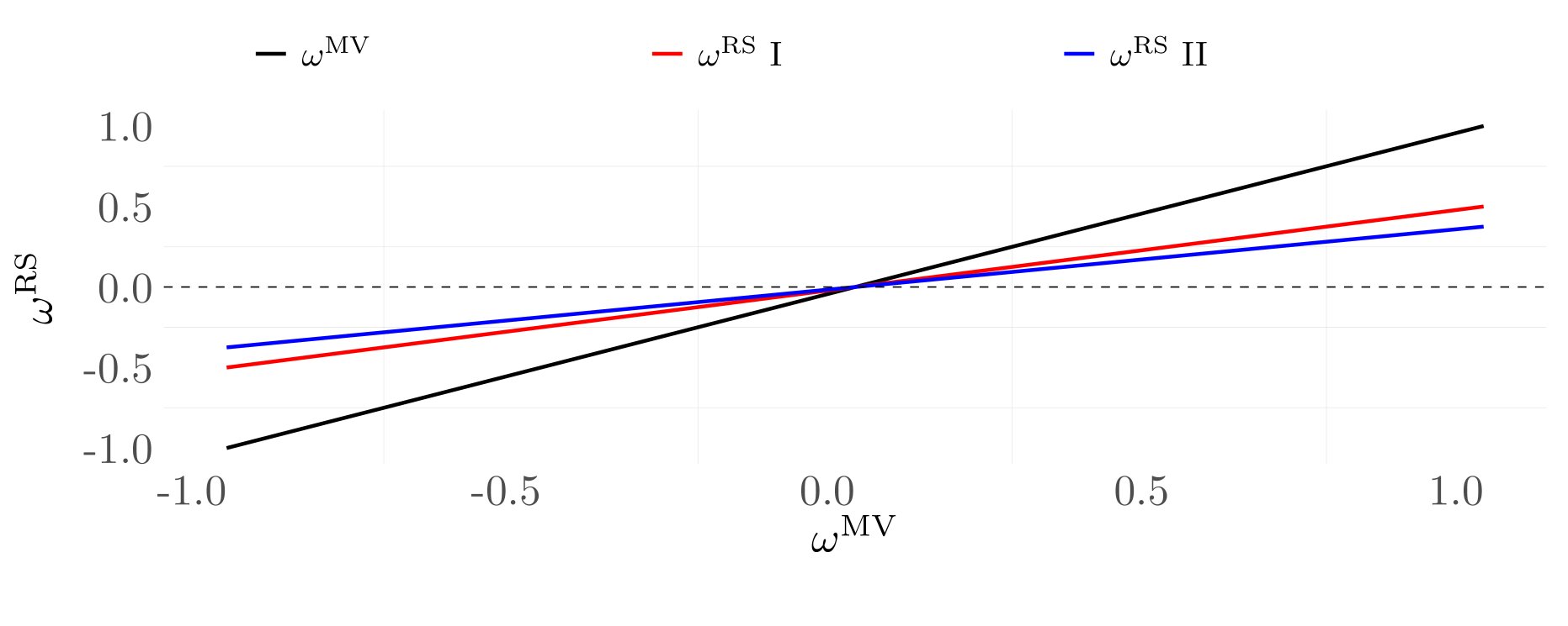
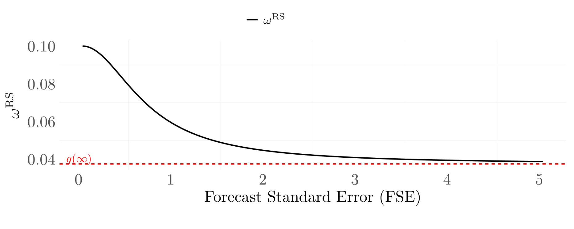
This figure shows the uncertainty averse (risk-sensitive) solution for the optimal portfolio weight in comparison with the standard mean-variance portfolio weight. In the upper panel, we hold the level of the forecast standard error (FSE) fixed and vary the mean-variance weight ($\omega^{\operatorname{MV}}$). The red line, $\omega^{\text{RS}}\text{ I}$ is constructed using $\omega_{\pi}^{\operatorname{MV}}=\omega^{\operatorname{MV}}$. The blue line, $\omega^{\text{RS}}\text{ II}$, is constructed using $\omega_{\pi}^{\operatorname{MV}}=0.5\times\omega^{\operatorname{MV}}$. In the lower panel, we consider the case where $\omega^{\operatorname{MV}}>a\omega_{\pi}^{\operatorname{MV}}$ and vary the forecast standard error (FSE).

To further shed light on the effect of incorporating forecast uncertainty into the shrinkage portfolio, we recall that $W_{1}=\operatorname{FSE}^{2}/(\operatorname{FSE}^{2}+v)$, hence $\omega^{\operatorname{RS}}$ can be written as an explicit function of $\operatorname{FSE}$ that shrinks the mean-variance portfolio: $\omega^{\operatorname{RS}}=g(\operatorname{FSE})$, where

$$g(s) := \left[\omega^{\operatorname{MV}}(1-W(s))+\omega^{\operatorname{MV}}_{\pi}W(s)\right]\frac{\sigma_{T}^{2}}{vW(s)+\sigma_{T}^{2}}\frac{\gamma}{\tau+\gamma}$$

$$W(s) := \frac{s^{2}}{s^{2}+v}.$$

The monotonicity of $g(\cdot)$ depends on the relative magnitude between $\omega^{\operatorname{MV}}$ and $a\times\omega_{\pi}^{\operatorname{MV}}$, where $a=\frac{\sigma_{T}^{2}}{v+\sigma_{T}^{2}}.$

As an illustration, consider the case $\omega^{\operatorname{MV}}>a\omega_{\pi}^{\operatorname{MV}}$, which means that the traditional MVE position suggests holding a “large” position in the risky asset. The upper panel of Figure 6 compares $\omega^{\operatorname{RS}}$ with $\omega^{\operatorname{MV}}$ as the latter increases with a fixed FSE. Clearly, $\omega^{\operatorname{RS}}$ increases linearly in $\omega^{\operatorname{MV}}$ but at a slower rate due to the linear shrinkage effect. The lower panel plots the $g(\cdot)$ function with respect to the forecast standard error. As FSE increases, the uncertainty-averse investor decreases her position in the risky asset, i.e., moving in the opposite direction relative to $\omega^{\operatorname{MV}}$. However, there is no region of complete non-participation. As forecast uncertainty increases, $\omega^{\operatorname{RS}}$ converges to a “discounted” MV portfolio that relies solely on prior beliefs:

$$g(\infty)=\omega_{\pi}^{\operatorname{MV}}\frac{\sigma_{T}^{2}}{v+\sigma_{T}^{2}}\frac{\gamma}{\tau+\gamma},$$

Essentially, when forecast uncertainty is extremely high, the portfolio is predominantly guided by prior beliefs, minimizing the impact of the predicted expected returns.

A.4.2 Multiple risky assets

We now extend the framework outlined in the previous subsection to the scenario of multiple risky assets. We obtain the pooled ML forecast $\widehat{z}_{T+1|T}$ for the $R$-dimensional expected return $z_{T+1|T}$. Let $\operatorname{SE}^{2}$ be the forecast covariance matrix of $\widehat{z}_{T+1|T}$, and let $\Sigma_{T}$ be the $R\times R$ covariance of $z_{T+1}-z_{T+1|T}$. We impose a multivariate normal prior $z_{T+1|T}\sim\mathcal{N}(\pi,v)$, where $v$ is an $R\times R$ prior covariance matrix, set to $v=g\Sigma_{T}$ for some $g>0$ as in Zellner’s $g$-prior. Then the posterior of the predictive density for the $N$-dimensional $z_{T+1}$ is $f_{T}(z_{T+1})\sim\mathcal{N}(\widetilde{z}_{T+1},\widetilde{\Sigma})$, where for $W_{1}=\operatorname{SE}^{2}(\operatorname{SE}^{2}+v)^{-1}$,

$$\widetilde{z}_{T+1}=(I-W_{1})\widehat{z}_{T+1|T}+W_{1}\pi,\quad\widetilde{\Sigma}=\Sigma_{T}+vW_{1}^{\prime}.$$

Now consider the problem: for $h_{T}\sim\mathcal{N}(\mu,\widetilde{\Sigma})$: (see Section B.4 for the proof)

$$\mbox{\boldmath$\omega$}^{\operatorname{RS}} := \arg\max_{\mbox{\boldmath$\omega$}\in\mathbb{R}^{N}}\min_{\mu\in\mathbb{R}^{N}}\mbox{\boldmath$\omega$}^{\prime}\mu-\frac{\gamma}{2}\mbox{\boldmath$\omega$}^{\prime}\widetilde{\Sigma}\mbox{\boldmath$\omega$}+\frac{1}{\tau}D(h_{T}||f_{T})$$ (A.7)

$$= \frac{\gamma}{\tau+\gamma}\widetilde{\Sigma}^{-1}\Sigma_{T}\left[(I-W_{1})^{\prime}\mbox{\boldmath$\omega$}^{\operatorname{MV}}+W_{1}^{\prime}\mbox{\boldmath$\omega$}^{\operatorname{MV}}_{\pi}\right]$$ (A.9)

where

$$\mbox{\boldmath$\omega$}^{\operatorname{MV}}=\Sigma_{T}^{-1}\widehat{z}_{T+1|T}\frac{1}{\gamma},\quad\mbox{\boldmath$\omega$}_{\pi}^{\operatorname{MV}}=\Sigma_{T}^{-1}\pi\frac{1}{\gamma}$$

are respective the mean-variance portfolios based on $\widehat{z}_{T+1|T}$ and $\pi$. Hence $\omega^{\operatorname{RS}}$ still conducts a double shrinkage: First, it shrinks $\mbox{\boldmath$\omega$}^{\operatorname{MV}}$ towards $\mbox{\boldmath$\omega$}^{\operatorname{MV}}_{\pi}$ due to the weight $W_{1}$. Secondly, it shrinks the overall portfolio to zero due to the $\widetilde{\Sigma}^{-1}\Sigma_{T}$.

Note that as $g\to\infty$, the prior becomes more diffuse and then $W_{1}\to 0$, hence more weights are imposed on $\mbox{\boldmath$\omega$}^{\operatorname{MV}}$. The resulting portfolio $\mbox{\boldmath$\omega$}^{\operatorname{RS}}$ becomes less robust to the forecast uncertainty in $\widehat{z}_{T+1|T}$. We shall see the impact of this in the empirical study.

Appendix B Technical Appendix

B.1 Intuition

In this subsection we briefly explain the technical intuition on how we derive the expression

$$\widehat{z}_{T+1|T}-z_{T+1|T}=\frac{1}{T}\sum_{t=1}^{T}\mathcal{C}_{t}+o_{P}(T^{-1/2})$$

and why the leading term $\mathcal{C}_{t}$ does not depend on the specific choice of the ML space.

The Riesz-representation plays a key role in the asymptotic analysis, and has been commonly used in the inferene for semiparametric models, e.g., Newey (1994); Shen (1997); Chen and Shen (1998); Chen and White (1999); Chernozhukov et al. (2018), among many others. The use of Riesz-representation allows to directly span the ML forecast using the least squares loss function, which also requires studying the object of interest in a Hilbert space. To do so, define an inner product:

$$\langle h_{1},h_{2}\rangle:=\frac{1}{NT}\sum_{it}\mathbb{E}h_{1}(x_{i,t-1})h_{2}(x_{i,t-1})$$

where the expectation is taken jointly with respect to the serial and cross-sectional distribution of $x_{i,t-1}$, treating $h_{1},h_{2}$ as fixed functions. Define

$$g_{NT,\mathcal{G}}:=\arg\min_{h\in\mathcal{G}_{\operatorname{DNN}}\cup\mathcal{G}_{B}}\|h-g\|_{L^{2}}^{2},$$

which is the best approximation to the true $g$ on the space $\mathcal{G}_{\operatorname{DNN}}\cup\mathcal{G}_{B}$ under the norm $\|_{L^{2}}$. Then $\mathcal{A}_{NT}:=\text{span}(\mathcal{G}_{\operatorname{DNN}}\cup\mathcal{G}_{B}-\{g_{NT,\mathcal{G}}\})$ is a finite dimensional Hilbert spaced endowed with the inner product $\langle\cdot,\cdot\rangle.$ Next, evaluated at the out-of-sample characteristics $x_{i,T}$, define a sequence of linear functionals:

$$\mathcal{T}_{i}(h):=h(x_{i,T}),\quad i=1,...,N.$$

Because $\mathcal{T}_{j}$ is a linear functional it is always bounded on the finite dimensional Hilbert space $\mathcal{A}_{NT}$. The Riesz representation theorem then implies that there is a function $m_{j}^{*}\in\mathcal{A}_{NT}$, called Riesz representer, so that

$$\mathcal{T}_{j}(h)=\langle h,m_{j}^{*}\rangle,\quad\forall h\in\mathcal{A}_{NT}.$$

The key fact to our argument is that $m^{*}_{j}$ does not depend on the specific machine learning space being used (whether $\mathcal{G}_{NT,\mathcal{G}}$ or $\mathcal{G}_{B}$) for $\widehat{z}_{T+1|T}$. It only depends on the joint distribution of $\{x_{i,t-1}\}$, the realization $\{x_{j,T}\}$ and the union space $\mathcal{G}_{\operatorname{DNN}}\cup\mathcal{G}_{B}$.

Next, using an argument for M-estimation (e.g. Theorem 3.2.5 of van der Vaart and Wellner (1996)), we show in Lemma 8 that uniformly for $j\leq N$,

$$\langle\widehat{g}-g,m^{*}_{j}\rangle=\frac{1}{NT}\sum_{it}e_{i,t}m^{*}_{j}(x_{i,t-1})+o_{P}(T^{-1/2}).$$

Then heuristically,

$$\widehat{z}_{T+1|T}-z_{T+1|T} = \sum_{j}w_{j}[\widehat{g}(x_{j,T})-g(x_{j,T})]=\sum_{j}w_{j}\mathcal{T}_{j}(\widehat{g}-g)$$

$$\approx \sum_{j}w_{j}\langle\widehat{g}-g,m_{j}^{*}\rangle$$

$$\approx \frac{1}{NT}\sum_{it}\sum_{j}w_{j}e_{i,t}m^{*}_{j}(x_{i,t-1}).$$

This yields the desired expansion with $\mathcal{C}_{t}\approx\frac{1}{N}\sum_{i}\sum_{j}w_{j}e_{i,t}m^{*}_{j}(x_{i,t-1})$. It is clear from this expression that $\mathcal{C}_{t}$ does not depend on the specific choice of the ML method.

B.2 Assumptions

We shall use two machine learning spaces: the “forecast ML” $\mathcal{G}_{\operatorname{DNN}}$, which is the space for deep neural networks, and the closed-form ML $\mathcal{G}_{B}$, which is the Fourier series to compute the standard error. Let $\mathcal{N}(\delta,\mathcal{G},\|.\|_{\infty})$ denote the entropy cover of $\mathcal{G}$, which is the smallest number of $\|.\|_{\infty}$-balls of radius $\delta$ to cover $\mathcal{G}$.

Assumption 1.

Conditioning on $X$, $(v_{t},u_{i,t})$ and are independent over time and are sub-Gaussian. Also suppose $x_{i,t-1}$ are independent across $i$.

Assumption 2.

The following conditions holds for $\mathcal{G}=\mathcal{G}_{\operatorname{DNN}}$, the neural network space.

1. There is $p(\mathcal{G})$ so that the covering number satisfies: for any $\delta>0$,

   $$\mathcal{N}(\delta,\mathcal{G},\|.\|_{\infty})\leq\left(\frac{CT}{\delta}\right)^{p(\mathcal{G})}.$$ (B.1)

2. Let

   $$\varphi_{\mathcal{G}}^{2}=\inf_{v\in\mathcal{G}}\sup_{h\in\{\tau_{T}g+\mathcal{G}\}\cup\{g\}}\|v-h\|_{\infty}^{2}.$$

   Suppose $\varphi_{\mathcal{G}}=o(T^{-1})$, $p(\mathcal{G})\log(NT)=o(T^{1/2})$ and $\varphi_{\mathcal{G}}p(\mathcal{G})\log(NT)=o(1)$.

3. Define the best approximation to the true $g$ function under the $\|.\|_{L^{2}}$-norm:

   $$g_{NT,\mathcal{G}}:=\arg\min_{h\in\mathcal{G}}\frac{1}{NT}\sum_{it}\mathbb{E}(h(x_{i,t-1})-g(x_{i,t-1}))^{2}.$$

   Suppose $\sqrt{T}\max_{j\leq N}|g_{NT,\mathcal{G}}(x_{j,T})-g(x_{j,T}))|=o_{P}(1)$.

The above assumption is well known to be satisfied by DNN for properly specified width and depth of the layers. Schmidt-Hieber (2020) show that a multilayer feedforward network with ReLu activation functions at each layer can well approximate a rich class of functions with compact support. It also follows from Anthony and Bartlett (2009) that (B.2) holds with $p(\mathcal{G}_{\operatorname{DNN}})$ as the pseudo dimension of the neural network, with $p(\mathcal{G}_{\operatorname{DNN}})=O(J^{2}L^{2})$, where $J,L$ are respectively the maximum width and depth of the network.

Assumption 3.

The following conditions holds for $\mathcal{G}=\mathcal{G}_{B}$, the Fourier series regression.

1. There is $p(\mathcal{G})$ so that the covering number satisfies: for any $\delta>0$,

   $$\mathcal{N}(\delta,\mathcal{G},\|.\|_{\infty})\leq\left(\frac{CT}{\delta}\right)^{p(\mathcal{G})}.$$ (B.2)

2. Let

   $$\varphi_{\mathcal{G}}^{2}=\inf_{v\in\mathcal{G}}\sup_{h\in\{\tau_{T}g+\mathcal{G}\}\cup\{g\}}\|v-h\|_{\infty}^{2}.$$

   Suppose $\varphi_{\mathcal{G}}=o(T^{-1})$, $p(\mathcal{G})\log(NT)=o(T^{1/2})$ and $\varphi_{\mathcal{G}}p(\mathcal{G})\log(NT)=o(1)$.

3. Define the best approximation to the true $g$ function under the $\|.\|_{L^{2}}$-norm:

   $$g_{NT,\mathcal{G}}:=\arg\min_{h\in\mathcal{G}}\frac{1}{NT}\sum_{it}\mathbb{E}(h(x_{i,t-1})-g(x_{i,t-1}))^{2}.$$

   Suppose $\sqrt{T}\max_{j\leq N}|g_{NT,\mathcal{G}}(x_{j,T})-g(x_{j,T}))|=o_{P}(1)$.

4. Let $J$ be the number of Fourier basis functions. Then $J^{5/2}=o(T)$ and $(\frac{p(\mathcal{G}_{G})\log(T)}{T}+\varphi_{\mathcal{G}_{G}})J^{2}\leq o(1)$.

To justify the above assumption, note that the Fouries basis can well approximate a Hölder class of smooth functions; and (B.2) holds with $p(\mathcal{G})\sim J$ being the number of basis functions.

B.3 Proofs

B.3.1 Proof of Theorem 1

For any generic function $h$, which may or may not be in $\mathcal{G}\in\{\mathcal{G}_{\operatorname{DNN}},\mathcal{G}_{1}\}$, let

$Q(h)=\frac{1}{TN}\sum_{it}(y_{i,t}-h(x_{i,t-1}))^{2}$ be the least squares loss function. Let

$$\psi_{\mathcal{G}}(h)=|Q(\pi_{\mathcal{G}}(h))-Q(h)|,\quad\pi_{\mathcal{G}}(h)=\arg\min_{v\in\mathcal{G}}\|v-h\|_{\infty}.$$ (B.3)

Here $\pi_{\mathcal{G}}(h)$ is the projection of function $h$ onto the learning space $\mathcal{G}$. In particular, if $h\in\mathcal{G}$ then $\pi_{\mathcal{G}}(h)=h$.

Theorem 1 is restated and proved by the following proposition.

Proposition 6.

Suppose $\sum_{i}|w_{i}|<\infty$. There are functions $m_{j}^{*}$, which is the same whether DNN or Fourier series are used as the predictor, so that for $\widehat{z}_{T+1}$ being either the DNN predictor or the Fourier series predictor,

$$\widehat{z}_{T+1}-z_{T+1|T} = \frac{1}{T}\sum_{t}\frac{1}{N}\sum_{i}\zeta^{*}(x_{i,t-1})\beta_{i,t-1}^{\prime}v_{t}+o_{P}(T^{-1/2})$$

$$\zeta^{*}(\cdot) := \sum_{j}w_{j}m_{j}^{*}(\cdot).$$

Proof.

Let $\mathcal{G}_{\operatorname{DNN}}$ be the DNN space and $\mathcal{G}_{B}$ denote the Fourier series space. Define $\mathcal{A}=\text{span}(\mathcal{G}_{\operatorname{DNN}}\cup\mathcal{G}_{B}-\{g\}),$ which is the closed linear span of $\mathcal{G}_{\operatorname{DNN}}\cup\mathcal{G}_{B}-g$ and $g$ is the true $g$ function. Also, define

$$g_{NT,\mathcal{G}}:=\arg\min_{h\in\mathcal{G}_{\operatorname{DNN}}\cup\mathcal{G}_{B}}\frac{1}{NT}\sum_{it}\mathbb{E}(h(x_{i,t-1})-g(x_{i,t-1}))^{2},$$

which is the best approximation to the true $g$ on the space $\mathcal{G}_{\operatorname{DNN}}\cup\mathcal{G}_{B}$ under the norm $\|_{L^{2}}$. Define $\mathcal{A}_{NT}=\text{span}(\mathcal{G}_{\operatorname{DNN}}\cup\mathcal{G}_{B}-\{g_{NT,\mathcal{G}}\})$. Then both $\mathcal{A}$ and $\mathcal{A}_{NT}$ are Hilbert spaces endowed with the inner product $\langle,\rangle$. Also $\mathcal{A}_{NT}$ is a finite dimensional space. Now define a sequence of linear functionals, evaluated at the out-of-sample $x_{j,T}$:

$$\mathcal{T}_{j}(h):=h(x_{j,T}),\quad j=1,...,N,\quad h\in\mathcal{A}\cup\mathcal{A}_{NT}.$$

Next we adopt the Riesz representation theorem on $\mathcal{A}_{NT}$. Because $\mathcal{T}_{j}$ is a linear functional, it is always bounded on the finite dimensional Hilbert space $\mathcal{A}_{NT}$. Hence the Riesz representation theorem implies that there is a function $m_{j}^{*}\in\mathcal{A}_{NT}$, called Riesz representer, so that

$$\mathcal{T}_{j}(h)=\langle h,m_{j}^{*}\rangle,\forall h\in\mathcal{A}_{NT}.$$

Hence $m_{j}^{*}$ only depends on the definition of the inner product and $\mathcal{A}_{NT}$, that is, the distribution of $\{x_{i,t-1}:t\leq T\}$ and the realization $x_{j,T}$, but does not depend on whether DNN or Fourier series were used to construct $\widehat{z}_{T+1}$. ($\mathcal{A}_{NT}$ is the same whether DNN or Fourier series were used.) We have two claims:

claim 1: $\langle m_{j}^{*},g_{NT,\mathcal{G}}-g\rangle=0$. This is because $g_{NT,\mathcal{G}}$ is the projection of $g$ on $\mathcal{A}_{NT}$ under the norm induced by the inner product, so it should be “orthogonal” to $m_{j}^{*}$ and any element in $\mathcal{A}_{NT}$.

claim 2: $\sqrt{T}\max_{j\leq N}|g_{NT,\mathcal{G}}(x_{j,T})-g(x_{j,T}))|=o_{P}(1)$, following from Assumption 1.

Then take $m_{j}=m_{j}^{*}$ in Lemma 8, and let $h=\widehat{g}-g_{NT,\mathcal{G}}\in\mathcal{A}_{NT}$,

$$\widehat{z}_{T+1|T}-z_{T+1|T} = \sum_{j}w_{j}[\widehat{g}(x_{j,T})-g(x_{j,T})]=\sum_{j}w_{j}\mathcal{T}_{j}(\widehat{g}-g)$$

$$= \sum_{j}w_{j}\mathcal{T}_{j}(\widehat{g}-g_{NT,\mathcal{G}})+\sum_{j}w_{j}[g_{NT,\mathcal{G}}(x_{j,T})-g(x_{j,T})]$$

$$= \sum_{j}w_{j}\langle\widehat{g}-g_{NT,\mathcal{G}},m_{j}^{*}\rangle+o_{P}(T^{-1/2})=\sum_{j}w_{j}\langle\widehat{g}-g,m_{j}^{*}\rangle+o_{P}(T^{-1/2})$$

$$=^{(a)} \frac{1}{NT}\sum_{it}\sum_{j}w_{j}e_{i,t}m^{*}_{j}(x_{i,t-1})+o_{P}(T^{-1/2})$$

$$=^{(b)} \frac{1}{T}\sum_{t}\frac{1}{N}\sum_{i}\zeta^{*}(x_{i,t-1})\beta_{i,t-1}^{\prime}v_{t}+L+o_{P}(T^{-1/2})$$

$$L := \frac{1}{NT}\sum_{it}\sum_{j}w_{j}u_{i,t}m^{*}_{j}(x_{i,t-1})=o_{P}(T^{-1/2}).$$

In the above (a) follows from Lemma 8; (b) is due to $\zeta^{*}(\cdot)=\sum_{j}w_{j}m_{j}^{*}(\cdot)$ and the definition of $e_{i,t}$.

∎

Lemma 7.

Write $\|g_{1}\|_{T}^{2}=\frac{1}{NT}\sum_{it}g_{1}(x_{i,t-1})^{2}$ and $\|g_{1}\|_{L^{2}}^{2}=\mathbb{E}\|g_{1}\|_{T}^{2}$ for any function $g_{1}$. Then

$$\|\widehat{g}-g\|_{L^{2}}^{2}\leq O_{P}(\frac{p(\mathcal{G})\log(T)}{T}+\varphi_{\mathcal{G}}).$$

Proof.

For notational simplicity, we write $\frac{1}{NT}\sum_{it}eg_{1}=\frac{1}{NT}\sum_{it}e_{i,t}g_{1}(x_{i,t-1})$ for any function $g_{1}$. Let $\zeta_{T}:=\|g-\pi g\|_{T}^{2}+2\frac{1}{NT}\sum_{it}e(g-\pi g)$. Then $Q(\widehat{g})\leq Q(\pi g)$ implies (for $\mathbb{E}$ taken with respect the distribution of $(e_{i,t},x_{i,t-1})$)

$$\|g-\widehat{g}\|_{L^{2}}^{2}\leq\mathbb{E}\frac{2}{NT}\sum_{it}e(\widehat{g}-g)+\mathbb{E}\zeta_{T}\leq\mathbb{E}\frac{2}{NT}\sum_{it}e(\widehat{g}-g)+O_{P}(\varphi_{\mathcal{G}}).$$

Suppose $m_{1},...,m_{K(\delta)}$ is a $\delta$-cover of $\mathcal{G}$ under the norm $\|m\|_{\infty}$ and $K(\delta):=\mathcal{N}(\delta,\mathcal{G},\|.\|_{\infty})$ as the covering number, where $\delta>0$ is to be determined. Then there is $m_{j}$ so that $\|m_{j}-\widehat{g}\|_{\infty}<\delta$. Now let $\mu_{j}(x)=[m_{j}(x)-g(x)]/\|m_{j}-g\|_{L^{2}}$.

Conditioning on $X$, $(v_{t},u_{i,t})$ and thus $e_{i,t}$ are independent over time and $e_{i,t}$ is sub-Gaussian. Then

$$\mathbb{E}\max_{j\leq K(\delta)}\frac{1}{NT}\sum_{it}e_{i,t}\mu_{j}(x_{i,t-1})\leq O(\sqrt{\frac{\log K(\delta)}{T}})=O(\sqrt{\frac{p(\mathcal{G})\log(CT/\delta)}{T}}).$$

If $\|\widehat{g}-g\|_{L^{2}}\leq T^{-9}$, then we are done. If $\|\widehat{g}-g\|_{L^{2}}>T^{-9}$, then set $\delta=T^{-9}$,

$$\mathbb{E}\frac{1}{NT}\sum_{it}e(\widehat{g}-g) \leq \mathbb{E}\max_{j}\frac{1}{NT}\sum_{it}e\mu_{j}\|m_{j}-g\|_{L^{2}}+\mathbb{E}\frac{1}{NT}\sum_{it}|e_{i,t}|\delta$$

$$\leq O(\sqrt{\frac{p(\mathcal{G})\log(CT/\delta)}{T}})[\delta+\|\widehat{g}-g\|_{L^{2}}]+O(\delta)$$

$$\leq O(\sqrt{\frac{p(\mathcal{G})\log(T)}{T}})\|\widehat{g}-g\|_{L^{2}}+O(T^{-9}).$$

Hence $\|g-\widehat{g}\|_{L^{2}}^{2}\leq O_{P}(\sqrt{\frac{p(\mathcal{G})\log(T)}{T}})\|\widehat{g}-g\|_{L^{2}}+O_{P}(T^{-9}+\varphi_{\mathcal{G}})$. This implies the result.

∎

Lemma 8.

Fix functions $m_{j}$ so that $\max_{j\leq N}\frac{1}{NT}\sum_{it}m_{j}(x_{i,t-1})^{2}=O_{P}(1)$. Let $\widehat{g}$ denote the minimizer of $Q(\cdot)$ on the space $\mathcal{G}$. Then uniformly for all $j=1,...,N$,

$$\langle\widehat{g}-g,m_{j}\rangle=\frac{1}{NT}\sum_{it}e_{i,t}m_{j}(x_{i,t-1})+o_{P}(T^{-1/2}).$$

Proof.

Recall $\psi_{\mathcal{G}}(h)=|Q(\pi(h))-Q(h)|$. For any deterministic sequence $\tau_{T}$, and function $m(x)$, consider a function $h:\mathbb{R}^{\dim(x)}\rightarrow\mathbb{R}$ so that

$$h_{j}(x):=\widehat{g}(x)+\tau_{T}m_{j}(x).$$

Then, $Q(\widehat{g})\leq Q(\pi h_{j})$ implies $Q(\widehat{g})-Q(h_{j})\leq\psi_{T}(h_{j}).$ Expand this inequality, and note that $y_{i,t}=g(x_{i,t-1})+e_{i,t}$,

$$-\tau_{T}^{2}\frac{1}{NT}\sum_{it}m_{j}(x_{i,t-1})^{2}+2\tau_{T}\underbrace{\left[\frac{1}{NT}\sum_{it}(g(x_{i,t-1})-\widehat{g}(x_{i,t-1}))m_{j}(x_{i,t-1})+\frac{1}{N}\sum_{it}e_{i,t}m_{j}(x_{i,t-1})\right]}_{\mathcal{M}_{j}}\leq\psi_{T}(h_{j})$$

where the left hand side of this inequality equals $Q(\widehat{g})-Q(h_{j}).$ Fix a positive sequence $\epsilon_{T}>0$ and respectively take value $\tau_{T}\in\{\epsilon_{T},-\epsilon_{T}\}$. Then the above inequality yields,

$$2|\mathcal{M}_{j}|\leq\epsilon_{T}\max_{j}\frac{1}{NT}\sum_{it}m_{j}(x_{i,t-1})^{2}+\psi_{T}(h_{j})/\epsilon_{T}.$$ (B.4)

We have $\psi(h_{j})\leq Q(\pi h_{j})-Q(h_{j})=\|h_{j}-\pi h_{j}\|_{T}^{2}+\frac{2}{N}\sum_{i}(y_{i,t}-h_{j})(h_{j}-\pi h_{j})\leq O_{P}(\varphi_{\mathcal{G}})=o_{P}(T^{-1}).$ This means $\sqrt{T}\max_{j}\psi_{T}(h_{j})=o_{P}(T^{-1/2})$. Then for $\epsilon_{T}:=\sqrt{\max_{j}\psi_{T}(h_{j})}$,

$$\sqrt{T}\max_{j}\psi_{T}(h_{j})=o_{P}(\epsilon_{T}),\quad\epsilon_{T}=o(T^{-1/2}).$$

For this choice of $\epsilon_{T}$, the right hand side of (B.4) is $o_{P}(T^{-1/2})$. This shows

$$A_{j}:=\frac{1}{NT}\sum_{it}(\widehat{g}(x_{i,t-1})-g(x_{i,t-1}))m_{j}(x_{i,t-1})=\frac{1}{NT}\sum_{it}e_{i,t}m_{j}(x_{i,t-1})+o_{P}(T^{-1/2})$$ (B.5)

uniformly for $j\leq N$.

Next, we show $A_{j}=\langle\widehat{g}-g,m_{j}\rangle+o_{P}(T^{-1/2})$ uniformly in $j\leq N$ by proving a conclusion similar to the stochastic equicontinuity. Let

$$G_{j}(v) := \frac{1}{NT}\sum_{it}(v(x_{i,t-1})-g(x_{i,t-1}))m_{j}(x_{i,t-1})-\mathbb{E}(v(x_{i,t-1})-g(x_{i,t-1}))m_{j}(x_{i,t-1})$$

$$\mathcal{C} := \{v\in\mathcal{G}:\|v\|_{L^{2}}^{2}<C\frac{p(\mathcal{G})\log T}{T}+C\varphi_{N}\}.$$

Lemma 7 shows $\widehat{g}\in\mathcal{C}$ with probability arbitrarily close to one. Hence

$$|A_{j}-\langle\widehat{g}-g,m_{j}\rangle|=|G_{j}(\widehat{g})|\leq\sup_{v\in\mathcal{C}}\max_{j\leq N}|G_{j}(v)|.$$

We now show the right hand side is $o_{P}(T^{-1/2})$ by establishing the stochastic equicontinuity. Let $p_{1},...,p_{K(\delta)}$ be a $\delta$-cover of $\mathcal{G}$ under the norm $\|p\|_{\infty}$. Let

$$h_{kj}(x):=[p_{k}(x)-g(x)]m_{j}(x)-\langle p_{k}-g,m_{j}\rangle,\quad\mu_{kj}(x)=h_{kj}(x)/\|h_{kj}\|_{L^{2}}.$$

Then $\mathbb{E}\mu_{kj}(x_{i,t-1})=0$; also $\mu_{kj}(x_{i,t-1})$ are independent across $i$. Also let $\mathcal{B}:=\{k:\exists v\in\mathcal{C},\|v-p_{k}\|_{\infty}<\delta\}$. Then set $\delta=T^{-1}$, for some $C>0$,

$$\max_{k\in\mathcal{B},j\leq N}\|h_{kj}\|_{L^{2}} \leq C\sup_{k\in\mathcal{B},j\leq N}\|p_{k}-g\|_{L^{2}}\leq C\sqrt{\frac{p(\mathcal{G})\log T}{T}}+C\sqrt{\varphi_{\mathcal{G}}}+C\delta\text{ (Cauchy-Schwarz)}$$

$$\max_{k\in\mathcal{B},j\leq N}|G_{j}(p_{k})| = \max_{k\in\mathcal{B},j\leq N}\left|\frac{1}{NT}\sum_{it}h_{kj}(x_{i,t-1})\right|=\max_{k\in\mathcal{B},j\leq N}\left|\frac{1}{NT}\sum_{it}\mu_{kj}(x_{i,t-1})\right|\|h_{kj}\|_{L^{2}}$$

$$\leq O_{P}(\sqrt{\frac{p(\mathcal{G})\log T}{T}}+\sqrt{\varphi_{\mathcal{G}}}+\delta)\sqrt{\frac{\log(K(\delta)N)}{T}}$$

$$\sup_{v\in\mathcal{C}}\max_{j}|G_{j}(v)| \leq \max_{p\in\mathcal{B},j\leq N}|G_{j}(p_{k})|$$

$$+\max_{j}\sup_{v\in\mathcal{C},\|v-p_{k}\|_{\infty}<\delta}|\frac{1}{NT}\sum_{it}(p_{k}(x_{i,t-1})-v(x_{i,t-1}))m_{j}(x_{i,t-1})-\langle p_{k}-v,m_{j}\rangle|$$

$$\leq O_{P}(\sqrt{\frac{p(\mathcal{G})\log T}{T}}+\sqrt{\varphi_{\mathcal{G}}}+\delta)\sqrt{\frac{\log(K(\delta)N)}{T}}+\delta=o_{P}(T^{-1/2}).$$

The last equality holds since $\log(K(\delta)N)=p(\mathcal{G})\log(NT),$ and $p(\mathcal{G})\log(NT)=o(T^{1/2})$ and $\varphi_{\mathcal{G}}p(\mathcal{G})\log(NT)=o(1)$. This implies uniformly in $j\leq N$,

$$\frac{1}{NT}\sum_{it}(\widehat{g}(x_{i,t-1})-g(x_{i,t-1}))m_{j}(x_{i,t-1})=\langle\widehat{g}-g,m_{j}\rangle+o_{P}(T^{-1/2}).$$

This finishes the proof.

∎

B.3.2 Proof of Theorem 2

Let $J$ be the number of Fourier series basis and suppose $J^{5/2}=o(T)$ and $(\frac{p(\mathcal{M})\log(T)}{T}+\varphi_{\mathcal{M}})J^{2}\leq o(1)$.

Let $\widehat{z}_{T+1|T}$ denote the DNN predictor, and let $\widehat{z}_{T+1|T,B}$ denote the Fourier series predictor. Proposition 6 show that

$$\widehat{z}_{T+1|T}-z_{T+1|T} = \frac{1}{T}\sum_{t}\frac{1}{N}\sum_{i}\zeta^{*}(x_{i,t-1})\beta_{i,t-1}^{\prime}v_{t}+o_{P}(T^{-1/2})$$ (B.6)

$$\widehat{z}_{T+1|T,B}-z_{T+1|T} = \frac{1}{T}\sum_{t}\frac{1}{N}\sum_{i}\zeta^{*}(x_{i,t-1})\beta_{i,t-1}^{\prime}v_{t}+o_{P}(T^{-1/2}).$$ (B.7)

Hence $\widehat{z}_{T+1|T}-z_{T+1|T}=\widehat{z}_{T+1|T,B}-z_{T+1|T}+o_{P}(T^{-1/2})$, which means the DNN predictor and Fourier series are asymptotically equivalent. In addition, it is easy to derive (using the analytical form of $\widehat{z}_{T+1|T,B}$): $\widehat{z}_{T+1|T,B}-z_{T+1|T}=\sum_{t=1}^{T}H^{\prime}\Phi_{t-1}^{\prime}\beta_{t-1}v_{t}+o_{P}(T^{-1/2}).$ Thus the DNN predictor satisfies:

$$\widehat{z}_{T+1|T}-z_{T+1|T}=\sum_{t=1}^{T}H^{\prime}\Phi_{t-1}^{\prime}\beta_{t-1}v_{t}+o_{P}(T^{-1/2}).$$

Define $\text{SE}(\widehat{z}_{T+1}):=\sqrt{\sum_{t=1}^{T}H^{\prime}\Phi_{t-1}^{\prime}\beta_{t-1}\operatorname{Cov}(f_{t})\beta_{t-1}^{\prime}\Phi_{t-1}H}.$ We now verify the Lindeberg condition, conditioning on $X$, which suffices to bound the fourth moment. Write $\text{SE}(\widehat{z}_{T+1})^{2}:=T^{-1}\sigma^{2}$ and $F_{t}:=H^{\prime}\Phi_{t-1}^{\prime}\beta_{t-1}v_{t}$. Then $\frac{1}{T}\sum_{t}\mathbb{E}(\|TF_{t}\|^{4}|X)<CJ^{5/2}$, because almost surely,

$$\frac{1}{T}\sum_{t}\|TH^{\prime}\Phi_{t-1}^{\prime}\beta_{t-1}\|^{4}\mathbb{E}(\|v_{t}\|^{4}|X)\leq C\|W^{\prime}\Phi_{T}(\frac{1}{TN}\Psi^{\prime}\Psi)^{-1}\|\frac{1}{TN}\sum_{it}\|\phi(x_{i,t-1})\|^{4}<CJ^{5/2}$$

given $W^{\prime}\Phi_{T}<C\sqrt{J}$, $\|(\frac{1}{TN}\Psi^{\prime}\Psi)^{-1}\|<C$, where $J$ is the number of Fourier series basis. If $J^{5/2}=o(T)$, $\frac{1}{\text{SE}(\widehat{z}_{T+1})^{2}}\sum_{t}\mathbb{E}(\|F_{t}\|^{2}1\{\|F_{t}\|>\epsilon\text{SE}(\widehat{z}_{T+1})\}|X)\leq\frac{1}{T}\frac{1}{T\sigma^{4}}\sum_{t}\mathbb{E}(\|TF_{t}\|^{4}|X)\to 0.$ Therefore,

$$\operatorname{SE}(\widehat{z}_{T+1})^{-1}(\widehat{z}_{T+1|T}-z_{T+1|T})\to^{d}\mathcal{N}(0,1).$$

It remains to prove $T(\widehat{\text{SE}}(\widehat{z}_{T+1})^{2}-\text{SE}(\widehat{z}_{T+1})^{2})=o_{P}(1)$.

Write $L^{\prime}:=W^{\prime}\Phi_{T}(\frac{1}{NT}\Psi^{\prime}\Psi)^{-1}$ and $s^{2}=\frac{1}{T}\sum_{t}L^{\prime}\frac{1}{N^{2}}\Phi_{t-1}^{\prime}e_{t}e_{t}^{\prime}\Phi_{t-1}L$. Then $\|L\|=O_{P}(\sqrt{J})$, and $\frac{1}{NT}\sum_{t}\|\widehat{e}_{t}-e_{t}\|^{2}=\frac{1}{NT}\sum_{it}|\widehat{g}(x_{i,t-1})-g(x_{i,t-1})|^{2}=O_{P}(\frac{p(\mathcal{M})\log(T)}{T}+\varphi_{\mathcal{M}}).$ Hence

$$T\widehat{\text{SE}}(\widehat{z}_{T+1})^{2}=\frac{1}{T}\sum_{t}L^{\prime}\frac{1}{N^{2}}\Phi_{t-1}^{\prime}\widehat{e}_{t}\widehat{e}_{t}^{\prime}\Phi_{t-1}L=s^{2}+O_{P}(\frac{p(\mathcal{M})\log(T)}{T}+\varphi_{\mathcal{M}})J^{2}=s^{2}+o_{P}(1).$$

Meanwhile, $\frac{1}{T}\sum_{t}L^{\prime}\frac{1}{N^{2}}\Phi_{t-1}^{\prime}\beta_{t-1}\operatorname{Cov}(f_{t})\beta_{t-1}^{\prime}\Phi_{t-1}L=T\text{SE}(\widehat{z}_{T+1})^{2}$, hence

$$s^{2}=\frac{1}{T}\sum_{t}L^{\prime}\frac{1}{N^{2}}\Phi_{t-1}^{\prime}\mathbb{E}(e_{t}e_{t}^{\prime}|\mathcal{F}_{t-1})\Phi_{t-1}L+o_{P}(1)=T\text{SE}(\widehat{z}_{T+1})^{2}+o_{P}(1).$$

B.3.3 Proof of Theorem 3: The Bootstrap

For ease of technical proofs, we prove for the asymptotic validity of the fully trained bootstrap neural networks. That is, let $(y_{i,t}^{*})$ denote the bootstrap data. We prove for the case when the bootstrap DNN $\widehat{g}^{*}(\cdot)$ is defined as:

$$\widehat{g}^{*}(\cdot)=\arg\min_{g\in\mathcal{G}_{\operatorname{DNN}}}\sum_{i=1}^{N}\sum_{t=1}^{T}(y^{*}_{i,t}-g(x_{i,t-1}))^{2},$$ (B.8)

where $\mathcal{G}_{\operatorname{DNN}}$ is the pooled-ML space, such as DNN.

Proof.

Here we focus on the DNN predictor, $\mathcal{G}=\mathcal{M}$. Let $\widehat{g}^{*}$ be the DNN estimator of $\widehat{g}$ using the bootstrap data. First, similar to Lemma 7, we can establish

$$\|\widehat{g}^{*}-\widehat{g}\|_{L^{2}}^{2}\leq O_{P^{*}}(\frac{p(\mathcal{G})\log(T)}{T}+\varphi_{\mathcal{G}}).$$

Hence $\widehat{g}^{*}\in\mathcal{C}$ with probability arbitrarily close to one. Also similar to the proof of (B.5), we can establish, for $m_{j}$ being the Riesz representer as in the proof of Proposition 6,

$$A_{j}^{*}:=\frac{1}{NT}\sum_{it}(\widehat{g}^{*}(x_{i,t-1})-\widehat{g}(x_{i,t-1}))m_{j}(x_{i,t-1})=\frac{1}{NT}\sum_{it}\widehat{e}^{*}_{i,t}m_{j}(x_{i,t-1})+o_{P^{*}}(T^{-1/2}).$$ (B.9)

Next, we show $A^{*}_{j}=\langle\widehat{g}-g,m_{j}\rangle+o_{P^{*}}(T^{-1/2})$ uniformly in $j\leq N$. The proof is slightly different from that in Lemma 8. Let

$$G_{j}(v_{1},v_{2}) := \frac{1}{NT}\sum_{it}(v_{1}(x_{i,t-1})-v_{2}(x_{i,t-1}))m_{j}(x_{i,t-1})-\mathbb{E}(v_{1}(x_{i,t-1})-v_{2}(x_{i,t-1}))m_{j}(x_{i,t-1}).$$

Hence

$$|A_{j}^{*}-\langle\widehat{g}^{*}-\widehat{g},m_{j}\rangle|=|G_{j}(\widehat{g}^{*},\widehat{g})|\leq\sup_{v_{1},v_{2}\in\mathcal{C}}\max_{j\leq N}|G_{j}(v_{1},v_{2})|.$$ (B.10)

Let $p_{1},...,p_{K(\delta)}$ be a $\delta$-cover of $\mathcal{G}$ under the norm $\|p\|_{\infty}$. Let

$$h_{kd,j}(x):=[p_{k}(x)-p_{d}(x)]m_{j}(x)-\langle p_{k}-p_{d},m_{j}\rangle,\quad\mu_{kd,j}(x)=h_{kd,j}(x)/\|h_{kd,j}\|_{L^{2}}.$$

Then $\mathbb{E}\mu_{kd,j}(x_{i,t-1})=0$; also $\mu_{kd,j}(x_{i,t-1})$ are independent across $i$. Also let $\mathcal{B}:=\{k:\exists v\in\mathcal{C},\|v-p_{k}\|_{\infty}<\delta\}$. Then set $\delta=T^{-1}$, for some $C>0$,

$$\max_{k,d\in\mathcal{B},j\leq N}\|h_{kd,j}\|_{L^{2}} \leq C\sup_{k,d\in\mathcal{B}}\|p_{k}-p_{d}\|_{L^{2}}\leq C\sqrt{\frac{p(\mathcal{G})\log T}{T}}+C\sqrt{\varphi_{\mathcal{G}}}+C\delta$$

$$\max_{k,d\in\mathcal{B},j\leq N}|G_{j}(p_{k},p_{d})| = \max_{k,d\in\mathcal{B},j\leq N}\left|\frac{1}{NT}\sum_{it}h_{kd,j}(x_{i,t-1})\right|=\max_{k,d\in\mathcal{B},j\leq N}\left|\frac{1}{NT}\sum_{it}\mu_{kd,j}(x_{i,t-1})\right|\|h_{kd,j}\|_{L^{2}}$$

$$\leq O_{P}(\sqrt{\frac{p(\mathcal{G})\log T}{T}}+\sqrt{\varphi_{\mathcal{G}}}+\delta)\sqrt{\frac{\log(K(\delta)N)}{T}}$$

$$\sup_{v_{1},v_{2}\in\mathcal{C}}\max_{j}|G_{j}(v_{1},v_{2})| \leq \max_{k,d\in\mathcal{B},j\leq N}|G_{j}(p_{k},p_{d})|+O_{P}(\delta)$$

$$\leq O_{P}(\sqrt{\frac{p(\mathcal{G})\log T}{T}}+\sqrt{\varphi_{\mathcal{G}}}+\delta)\sqrt{\frac{\log(K(\delta)N)}{T}}+\delta=o_{P}(T^{-1/2}).$$

Combining with (B.9)(B.10), for $\widehat{e}_{i,t}^{*}=\widehat{e}_{i,t}\eta_{t}^{*}$,

$$\langle\widehat{g}^{*}-\widehat{g},m_{j}\rangle=\frac{1}{NT}\sum_{it}\widehat{e}^{*}_{i,t}m_{j}(x_{i,t-1})+o_{P^{*}}(T^{-1/2}).$$

Next, for the same functional $\mathcal{T}_{j}$ and the Riesz representer $m_{j}=m_{j}^{*}$ in the proof of Proposition 6 and $\zeta^{*}=\sum w_{j}m_{j}^{*}$,

$$\widehat{z}^{*}_{T+1|T}-\widehat{z}_{T+1|T} = \sum_{j}w_{j}[\widehat{g}^{*}(x_{j,T})-\widehat{g}(x_{j,T})]=\sum_{j}w_{j}\mathcal{T}_{j}(\widehat{g}^{*}-\widehat{g})=\sum_{j}w_{j}\langle\widehat{g}^{*}-\widehat{g},m_{j}^{*}\rangle$$

$$= \frac{1}{NT}\sum_{it}\sum_{j}w_{j}\widehat{e}_{i,t}\eta^{*}_{t}m^{*}_{j}(x_{i,t-1})+o_{P^{*}}(T^{-1/2})$$

$$= \frac{1}{NT}\sum_{it}\widehat{e}_{i,t}\eta^{*}_{t}\zeta^{*}(x_{i,t-1})+o_{P^{*}}(T^{-1/2}).$$

Next, $\mathbb{E}\eta_{t}^{*}=0$ and $\operatorname{Var}^{*}(\eta_{t}^{*})=1$. Let $\widetilde{\zeta}_{t-1}$ be the $N$-vector of $\zeta^{*}(x_{i,t-1})$. Then

$$\widehat{\operatorname{SE}}_{inf}^{*2} := \frac{1}{T^{2}}\sum_{t}(\frac{1}{N}\widehat{e}_{t}^{\prime}\widetilde{\zeta}_{t-1})^{2}=\frac{1}{T^{2}}\sum_{t}(\frac{1}{N}e_{t}^{\prime}\widetilde{\zeta}_{t-1})^{2}+o_{P}(T^{-1})$$

$$= \frac{1}{T^{2}}\sum_{t}(\frac{1}{N}\widetilde{\zeta}^{\prime}_{t-1}\beta_{t-1}v_{t})^{2}+o_{P}(T^{-1})={\operatorname{SE}}_{inf}^{2}+o_{P}(T^{-1})$$

$${\operatorname{SE}}_{inf}^{2} := \frac{1}{T^{2}}\sum_{t}\frac{1}{N^{2}}\widetilde{\zeta}^{\prime}_{t-1}\beta_{t-1}\operatorname{Cov}(v_{t})\beta_{t-1}^{\prime}\widetilde{\zeta}_{t-1}.$$

This shows $c_{inf}:=\operatorname{SE}_{inf}^{-1}\widehat{\operatorname{SE}}_{inf}^{*}\to^{P}1$ because $\sqrt{T}\operatorname{SE}_{inf}>c>0$. Meanwhile,

$$\operatorname{SE}_{inf}^{-1}(\widehat{z}^{*}_{T+1|T}-\widehat{z}_{T+1|T}) = c_{inf}\widehat{\operatorname{SE}}_{inf}^{*-1}(\widehat{z}^{*}_{T+1|T}-\widehat{z}_{T+1|T})$$

$$= \left[\frac{1}{T^{2}}\sum_{t}(\frac{1}{N}\widehat{e}_{t}^{\prime}\widetilde{\zeta}_{t-1})^{2}\right]^{-1/2}\frac{1}{NT}\sum_{it}\widehat{e}_{i,t}\eta^{*}_{t}\zeta^{*}(x_{i,t-1})+o_{P^{*}}(1)$$

$$\to^{d^{*}} \mathcal{N}(0,1).$$

In addition, (B.6) shows $\operatorname{SE}_{inf}^{-1}(\widehat{z}_{T+1|T}-z_{T+1|T})\to^{d}\mathcal{N}(0,1).$ Let $q^{*}_{\alpha}$ be the bootstrap critical value of $|\widehat{z}^{*}_{T+1|T}-\widehat{z}_{T+1|T}|$ so that $P^{*}(|\widehat{z}^{*}_{T+1|T}-\widehat{z}_{T+1|T}|\leq q^{*}_{\alpha})=1-\alpha$, where $P^{*}$ denotes the probability measure with respect to the bootstrap distribution (i.e., the distribution of $\{\eta_{t}^{*},t\leq T\}$ conditional on the data). Then

$$P(|\widehat{z}_{T+1|T}-z_{T+1|T}|\leq q^{*}_{\alpha}) = P(|\operatorname{SE}_{inf}^{-1}(\widehat{z}_{T+1|T}-z_{T+1|T}|\leq\operatorname{SE}^{-1}_{inf}q^{*}_{\alpha})$$

$$= P^{*}(|\operatorname{SE}_{inf}^{-1}(\widehat{z}^{*}_{T+1|T}-\widehat{z}_{T+1|T})|\leq\operatorname{SE}^{-1}_{inf}q^{*}_{\alpha})+o_{P}(1)$$

$$= 1-\alpha+o_{P}(1).$$

∎

B.3.4 Proof of Theorem 4

Proof.

The constraint MV problem is $\max_{\omega}\min_{\mu}F(\omega,\mu)$, subject to $|\mu-\widehat{z}_{Z+1|T}|\leq q$, where $F(\omega,\mu)=\mbox{\boldmath$\omega$}^{\prime}\mu-\frac{\gamma}{2}\mbox{\boldmath$\omega$}^{\prime}\Sigma_{T}\mbox{\boldmath$\omega$}.$ For the inner problem, $\min_{\mu_{i}}\omega_{i}\mu_{i}$ subject to $|\mu_{i}-\widehat{z}_{T+1|T,i}|\leq q_{\alpha,i}$, the minimum is $\omega_{i}(\widehat{z}_{T+1|T,i}-\operatorname{sgn}(\omega_{i})q_{\alpha,i})=\omega_{i}\widehat{z}_{T+1|T,i}-|\omega_{i}|q_{\alpha,i}$. This leads to the designated result.

In the one dimensional case, the problem is equivalent to

$$\min_{\omega}\frac{\gamma}{2}\omega^{2}\sigma^{2}-\omega\widehat{z}_{T+1|T}+q|\omega|$$

which is also equivalent to $\min_{\omega}\frac{\gamma\sigma^{2}}{2}[\omega-\omega^{\operatorname{MV}}]^{2}+q|\omega|$. The solution is well known to be the soft thresholding operator given in the theorem.

∎

B.4 Proof of (A.1), (A.6) and (A.7)

Proof of Expression (A.1).

Proof.

For the case $R=2$, $\min_{\mbox{\boldmath$\omega$}=(\omega,1-\omega)}F(\omega)$, where

$F(\omega)=\frac{\gamma}{2}\mbox{\boldmath$\omega$}^{\prime}\Sigma_{T}\mbox{\boldmath$\omega$}-\omega\widehat{z}_{T+1|T,1}-(1-\omega)\widehat{z}_{T+1|T,2}+q_{\alpha,1}|\omega|+q_{\alpha,2}|1-\omega|.$ This function is piecewise quadratic on the regions $(-\infty,0],[0,1],$ and $[1,\infty)$. We define and verify that

$$\arg\min_{\omega>1}F(\omega) = \max\{A,1\},\quad\text{where}\quad A=\omega_{1}^{\operatorname{MV}}-c_{0}(q_{\alpha,1}+q_{\alpha,2})$$

$$\arg\min_{\omega<0}F(\omega) = \min\{C,0\},\quad\text{where}\quad C=\omega_{1}^{\operatorname{MV}}+c_{0}(q_{\alpha,1}+q_{\alpha,2})$$

$$\arg\min_{0<\omega<1}F(\omega) = 1\{0<B<1\}B+1\{B>1\}\quad\text{where}\quad B=\omega_{1}^{\operatorname{MV}}-c_{0}(q_{\alpha,1}-q_{\alpha,2})$$

$$\omega_{1}^{\operatorname{MV}} = c_{0}\left[\widehat{z}_{T+1|T,1}-\widehat{z}_{T+1|T,2}-\gamma(\operatorname{Cov}(z_{T+1,1},z_{T+1,2})-\operatorname{Var}(z_{T+1,2}))\right]$$

where $c_{0}=\gamma^{-1}\operatorname{Var}(z_{T+1,1}-z_{T+1,2})^{-1}$. Note that $C>B>A$. Also write $\omega_{2}^{\operatorname{MV}}=1-\omega_{1}^{\operatorname{MV}}$. Let the optimal solution be $\omega_{1}^{*}$, and $\omega_{2}^{*}=1-\omega_{1}^{*}$. Hence we have the following cases:

Case 1. $A>1$, which is $\omega_{2}^{\operatorname{MV}}<-c_{0}(q_{\alpha,1}+q_{\alpha,2})$, then $\omega_{1}^{*}=A$, and

$\omega_{2}^{*}=\omega_{2}^{\operatorname{MV}}+c_{0}(q_{\alpha,1}+q_{\alpha,2})$.

Case 2. $B>1>A$, which is $-c_{0}(q_{\alpha,1}+q_{\alpha,2})<\omega_{2}^{\operatorname{MV}}<c_{0}(q_{\alpha,2}-q_{\alpha,1})$, then $\omega_{1}^{*}=1$.

Case 3. $0<B<1$, which is $\omega_{1}^{\operatorname{MV}}>c_{0}(q_{\alpha,1}-q_{\alpha,2})$ and $\omega_{2}^{\operatorname{MV}}>c_{0}(q_{\alpha,2}-q_{\alpha,1})$, then $\omega_{1}^{*}=B$, and $\omega_{2}^{*}=1-B=\omega_{2}^{\operatorname{MV}}-c_{0}(q_{\alpha,2}-q_{\alpha,1})$.

Case 4. $C>0>B$, which is $-c_{0}(q_{\alpha,1}+q_{\alpha,2})<\omega_{1}^{\operatorname{MV}}<c_{0}(q_{\alpha,1}-q_{\alpha,2})$, then $\omega_{1}^{*}=0$.

Case 5. $C<0$, which is $\omega_{1}^{\operatorname{MV}}<-c_{0}(q_{\alpha,1}+q_{\alpha,2})$, then $\omega_{1}^{*}=C$.

Hence for $k,j\in\{1,2\}$ and $k\neq j$,

When $\omega_{1}^{\operatorname{MV}}<-c_{0}(q_{\alpha,1}+q_{\alpha,2})$, then $\omega_{k}^{*}=\omega_{1}^{\operatorname{MV}}+c_{0}(q_{\alpha,1}+q_{\alpha,2})$.

When $-c_{0}(q_{\alpha,1}+q_{\alpha,2})<\omega_{1}^{\operatorname{MV}}<c_{0}(q_{\alpha,k}-q_{\alpha,j})$, then $\omega_{k}^{*}=0$.

When $\omega_{1}^{\operatorname{MV}}>c_{0}(q_{\alpha,1}-q_{\alpha,2})$ and $\omega_{2}^{\operatorname{MV}}>c_{0}(q_{\alpha,2}-q_{\alpha,1})$, then $\omega_{k}^{*}=\omega_{1}^{\operatorname{MV}}-c_{0}(q_{\alpha,k}-q_{\alpha,j})$.

∎

Proof of Expressions (A.6), (A.7)

Proof.

(A.6) is a special case of (A.7). Hence we directly prove the latter. The conditional distribution of $z_{T+1}|\widehat{z}_{T+1|T}$ is normal. Also, $(z_{T+1|T},\widehat{z}_{T+1|T})$ is jointly normal, we have

$$\mathbb{E}(z_{T+1}|\widehat{z}_{T+1|T})=\mathbb{E}[\mathbb{E}(z_{T+1}|\widehat{z}_{T+1|T},z_{T+1|T})|\widehat{z}_{T+1|T}]=\mathbb{E}(z_{T+1|T}|\widehat{z}_{T+1|T})=(I-W_{1})\widehat{z}_{T+1|T}+W_{1}\pi$$

where $W_{1}=\operatorname{SE}^{2}(\operatorname{SE}^{2}+v)^{-1}.$ Also,

$$\begin{pmatrix}z_{T+1|T}\\ \widehat{z}_{T+1|T}\end{pmatrix}\sim\mathcal{N}\left(\begin{pmatrix}\pi\\ \pi\end{pmatrix},\begin{pmatrix}v&v\\ v&\operatorname{SE}^{2}+v\end{pmatrix}\right).$$

Hence $\operatorname{Var}(z_{T+1|T}|\widehat{z}_{T+1|T})=v-v(\operatorname{SE}^{2}+v)^{-1}v=vW_{1}^{\prime}=W_{1}v,$ and thus

$$\widetilde{\Sigma} = \operatorname{Var}(z_{T+1}|\widehat{z}_{T+1|T})=\mathbb{E}[\operatorname{Var}(z_{T+1}|z_{T+1|T})|\widehat{z}_{T+1|T}]+\operatorname{Var}(z_{T+1|T}|\widehat{z}_{T+1|T})$$

$$= \Sigma_{T}+\operatorname{Var}(z_{T+1|T}|\widehat{z}_{T+1|T})=\Sigma_{T}+(I-W_{1})\operatorname{SE}^{2}=\Sigma_{T}+vW_{1}^{\prime}.$$

Note that for two multivariate normal densities with the same covariance $\widetilde{\Sigma}$, the Kullback–Leibler divergence is

$$D(h_{T}||f_{T})=\frac{1}{2}(\mu-\widetilde{z}_{T+1})^{\prime}\widetilde{\Sigma}^{-1}(\mu-\widetilde{z}_{T+1}).$$

Hence $\mbox{\boldmath$\omega$}^{RS}:=\arg\max_{\mbox{\boldmath$\omega$}\in\mathbb{R}^{N}}\min_{\mu\in\mathbb{R}^{N}}L(\mbox{\boldmath$\omega$},\mu)$ where

$$L(\mbox{\boldmath$\omega$},\mu)=\mbox{\boldmath$\omega$}^{\prime}\mu-\frac{\gamma}{2}\mbox{\boldmath$\omega$}^{\prime}\widetilde{\Sigma}\mbox{\boldmath$\omega$}+\frac{1}{\tau}D(h_{T}||f_{T}).$$

We have $\min_{\mu\in\mathbb{R}^{N}}L(\mbox{\boldmath$\omega$},\mu)=\mbox{\boldmath$\omega$}^{\prime}\widetilde{z}_{T+1}-\frac{\gamma+\tau}{2}\mbox{\boldmath$\omega$}^{\prime}\widetilde{\Sigma}\mbox{\boldmath$\omega$}$. Maximizing it yields

$$\mbox{\boldmath$\omega$}^{RS}=\widetilde{\Sigma}^{-1}\widetilde{z}_{T+1}\frac{1}{\tau+\gamma}.$$

Recall that $\widetilde{z}_{T+1}=(1-W_{1})\widehat{z}_{T+1|T}+W_{1}\pi$, $\mbox{\boldmath$\omega$}^{\operatorname{MV}}=\Sigma_{T}^{-1}\widehat{z}_{T+1|T}\frac{1}{\gamma}$ and

$\mbox{\boldmath$\omega$}^{RS}_{\pi}=\Sigma_{T}^{-1}\pi\frac{1}{\gamma}$. Also, for any constant $c$, if $v=c\Sigma_{T}$, then $W_{1}\Sigma_{T}=\Sigma_{T}W_{1}^{\prime}$, both sides equal $\Sigma_{T}-c\Sigma_{T}(\operatorname{SE}^{2}+c\Sigma_{T})^{-1}\Sigma_{T}$. Hence

$$\mbox{\boldmath$\omega$}^{RS}=\frac{\gamma}{\tau+\gamma}\widetilde{\Sigma}^{-1}\Sigma_{T}\left[(I-W_{1})^{\prime}\mbox{\boldmath$\omega$}^{\operatorname{MV}}+W_{1}^{\prime}\mbox{\boldmath$\omega$}^{\operatorname{MV}}_{\pi}\right].$$

In the one-dimensional case, this implifies to

$$\omega^{RS}=\frac{\gamma}{\tau+\gamma}g(W_{1}),\quad g(W_{1}):=\frac{\sigma^{2}_{T}}{\sigma_{T}^{2}+vW_{1}}\left[(1-W_{1})\omega^{\operatorname{MV}}+W_{1}\omega^{\operatorname{MV}}_{\pi}\right].$$

In addition, $W_{1}=\operatorname{SE}^{2}/(\operatorname{SE}^{2}+v)$, which is monotonically increasing in $\operatorname{SE}$. Hence the monotonicity of $\omega^{RS}$ with respect to $\operatorname{SE}$ is determined by the monotonicity of $g(\cdot)$. It can be rewritten as

$$g(W_{1})=c+\frac{\sigma_{T}^{2}}{v}\frac{v+\sigma_{T}^{2}}{\sigma_{T}^{2}+vW_{1}}[\omega^{\operatorname{MV}}-\frac{\sigma_{T}^{2}}{v+\sigma_{T}^{2}}\omega_{\pi}^{\operatorname{MV}}].$$

Hence $g(\cdot)$ is increasing if and only if $\omega^{\operatorname{MV}}<\frac{\sigma_{T}^{2}}{v+\sigma_{T}^{2}}\omega_{\pi}^{\operatorname{MV}}$. ∎

References

- Allena (2021) Allena, R. (2021). Confident risk premiums and investments using machine learning uncertainties. Available at SSRN 3956311.