Is directed percolation class for synchronization transition robust with multi-site interactions?
Abstract
Coupled map lattice with pairwise local interactions is a well-studied system. However, in several situations, such as neuronal or social networks, multi-site interactions are possible. In this work, we study the coupled Gauss map in one dimension with 2-site, 3-site, 4-site and 5-site interaction. This coupling cannot be decomposed in pairwise interactions. We coarse-grain the variable values by labeling the sites above as up spin (+1) and the rest as down spin (-1) where is the fixed point. We define flip rate as the fraction of sites such that and persistence as the fraction of sites such that for all . The dynamic phase transitions to a synchronized state is studied above quantifiers. For 3 and 5 sites interaction, we find that at the critical point, with and with . They match the directed percolation (DP) class. Finite-size and off-critical scaling is consistent with DP class. For 2 and 4 site interactions, the exponent and behavior of at critical point changes. Furthermore, we observe logarithmic oscillations over and above power-law decay at the critical point for 4-site coupling. Thus multi-site interactions can lead to new universality class(es).
1 Introduction
A complex network has many interacting components that show the various range of dynamical behaviourandreev2019chimera ; costa2011analyzing . Such a system is applicable in many real-world systems, including the spreading of diseases in the populations cliff2019network , complex biological pathways bhalla1999emergent , social networks kanawati2015multiplex , neuronal networks andreev2019chimera ; mishra2018dragon etc. Dynamical systems on such networks could be coupled differential equations, coupled maps (CML), or cellular automata with a decreasing degree of complexity. Most of these models involve pairwise interactions between different elements. However, there are many systems where multi-site interaction is possible. This higher-order interaction is usually more complex and studied in many fields of science such as physics estrada2006subgraph , mathematics chodrow2020configuration , and computer science karypis1997multilevel . For instance, higher-order interactions are useful for modeling the functional brain connectionspetri2014homological . In this work, we study coupled maps with higher-order interactions. Map-based models have less computational cost and can reveal qualitative features. Such interactions can change the nature of dynamic phase transitions. Higher-order Kuramoto model can lead to explosive synchronization millan2020explosive . This is a discontinuous transition. The self-organized behavior of coupled-phase oscillators with many-body interaction is studied in skardal2020higher . This coupling reproduces the rapid synchronization in many valid biological networks. It has hysteresis and bistability indicating first-order transition. Such multi-site couplings are often studied on simplicial geometries gambuzza2021stability ; bhattacharya2021higher ; salnikov2018simplicial ; ghorbanchian2021higher . There are several reports of first-order transition in systems with simplicial couplingsmillan2020explosive ; chutani2021hysteresis ; kachhvah2022first ; matamalas2020abrupt ; jalan2022multiple . CML of logistic maps or neuronal maps with simplicial coupling is studied in naval ; perc1 . The above systems, many of which have real-world applications, motivate us to study the higher-order interaction in a system of coupled chaotic maps.
In particular, we study the transition to synchronization. We study CML with multi-site interaction. In this model, we study coupled map lattice with 2-site, 3-site, 4-site, and 5-site interaction. We retain the one-dimensional nature of underlying topology so that it is possible to compare it with one-dimensional transitions. Firstly, we find that the nature of the transition can be continuous and not necessarily explosive. Standard finite-size scaling is observed. (In explosive synchronization, it is claimed that the finite-size scaling is atypicald2019explosive .) All exponents including relatively less universal persistence exponent match with expected values for one-dimensional DP for the 3-site and 5-site interaction. The situation changes for the 2-site or 4-site interaction.
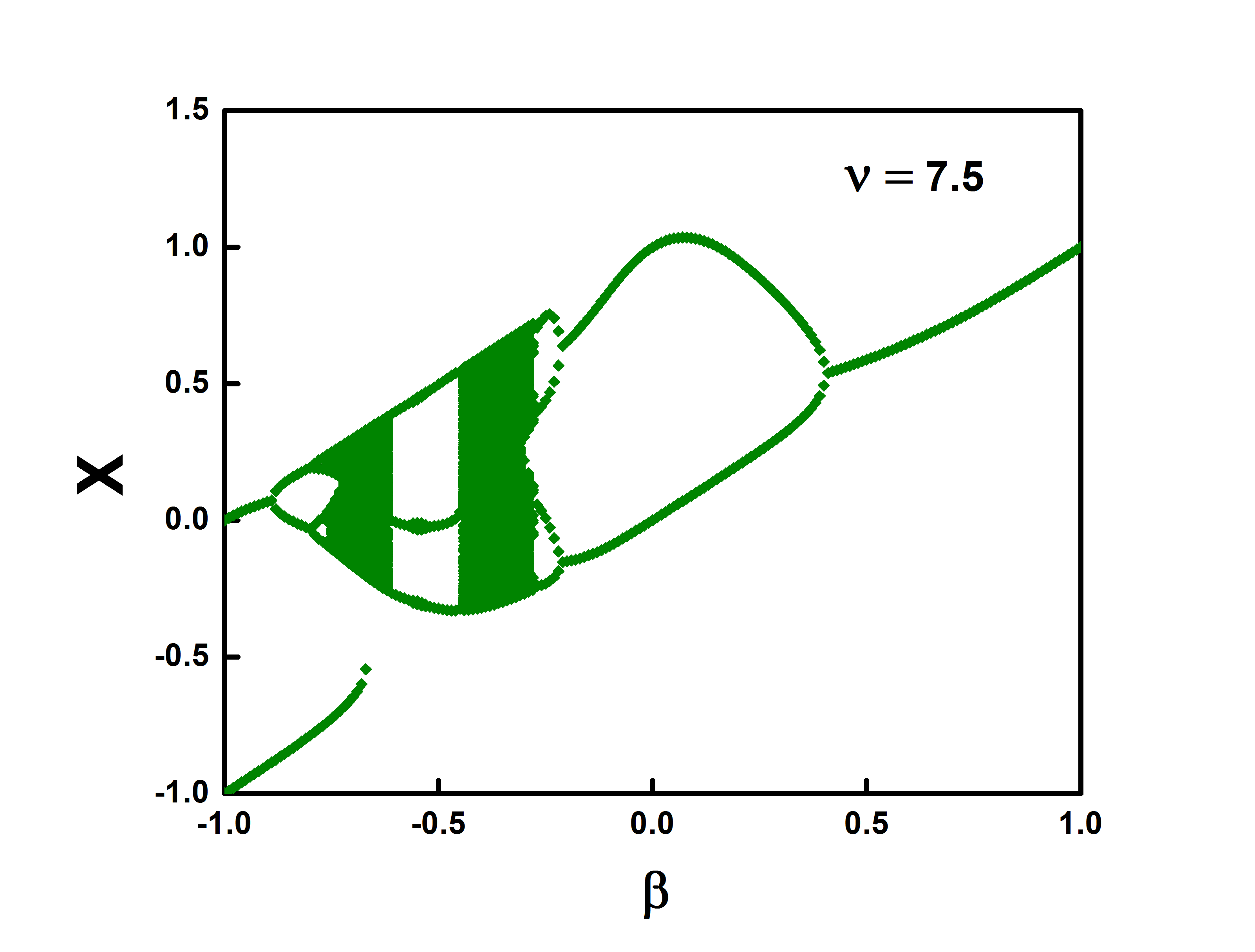
The Gauss map is a map based on the Gaussian exponential function patidar2006co . Unlike logistic, tent, or circle maps, this is a map defined on the entire real line and not an interval. Such maps are relatively less studied. On changing the map parameter values, this map shows the diverse range of dynamical behaviour including reverse period doubling, period adding and chaos. In standard form, it can be defined as:
| (1) |
Where and are the control parameters of the given map. We plot the bifurcation diagram of the Gauss map for [see Fig.1]. We plot all sites as a function of map parameter . The bifurcation plot displays distinct dynamical behavior including the reverse period-doubling, period-adding and chaos.
We study the CML with multi-site interaction in the Gauss map with positive coupling. Our studies are the viewpoint of phase transition, and this phase transition is identified by the appropriate order parameter. We consider local persistence and flip rate as order parameters. Persistence is the probability that a nonequilibrium field value does not change the sign up to time during stochastic evolution majumdar1999persistence . This is a non-Markovian quantity and experimental investigations are difficult for obvious reasons. In several systems, persistence decays algebraically with time at the critical point as where is the decay exponent known as the persistence exponent. We need the knowledge of entire time evolution to find this quantity.
For CML, transition to a frozen or partially frozen state in a coarse-grained sense can be characterized by persistence and power-law behaviour may be obtained only at the critical coupling. However, the persistence exponent is not universal. As noted below, several systems in the DP universality class have persistence exponent , and several systems in directed Ising universality have persistence exponent unity shambharkar2019universality . The persistence exponent in the DP model such as the Domany-Kinzel model hinrichsen1998numerical , Ziff-Gulari-Barshed model albano2001numerical , site percolation fuchs2008local and circle map menon2003persistence ; jabeen2005dynamic is observed to be . (We note that the synchronization transition between two coupled CML is found to be in bounded KPZ universality class for smooth mapsahlers . But, we focus on a single CML in this work.) The transition to a random pattern is frozen in the coarse-grained state (not synchronized) can be in DP universality class in CML pakhare2020novel ; pratik1 and shows persistence exponent close to . Although not universal, we can observe the same persistence exponent in a significant set of models belonging to the same universality class. Hence, it is important. In the above cases of coupled maps, flip rate is studied as a measure of lattice activity at a given time . Recently, a new universality class pertaining to transition to a period absorbing state has been observed in coupled map lattice and has been investigated using the flip rate as a quantifierpratik1 . (It is also modeled by the cellular automata model in divya1 .) We use the similar measure here. We denote sites with a variable value greater than a fixed point as spin (+1) and those with a value less than a fixed point as spin (-1). For the case of period-3 synchronization, flip rate is defined as the fraction of sites that change their spin state from state at time pratik1 . If the underlying coarse-grained periodicity is 2, it is the fraction of sites that changed its state at time from the state at naval ; pakhare2020novel . Thus, any departure from the expected underlying dynamics is the flip rate. In our case, the flip rate is the fraction of sites that change their spin state at from the previous state at .
DP is the most widely observed universality class in the nonequilibrium system from the viewpoint of phase transition from the active state to the absorbing state. It is observed in several systems including transition to turbulence hof2023directed or transition between two turbulent states of electroconvection in nematic liquid crystals takeuchi2009experimental . Janssen–Grassberger conjecture janssen1981nonequilibrium ; grassberger1981phase stated the conditions for DP transition as grassberger1981phase “the universality class of DP contains all continuous transitions from a dead or absorbing state to an active one with a single scalar order parameter, provided the dead state is not degenerate and provided some technical points are fulfilled: short-range interactions both in space and time, the nonvanishing probability for any active state to die locally, translational invariance (absence of frozen randomness), and absence of multicritical points”. The question is whether all these conditions are necessary and what happens if we relax some or all of them. Relaxation in some of these conditions still leads to the directed percolation universality classbhoyar2022robustness . Most of the models studied have pairwise interactions. We study interaction that cannot be decomposed as pairwise interaction and check the universality class of absorbing state transition in this system.
For CML with pairwise interaction, there are numerous instances of dynamic transitions in the DP universality class. For the coupled Gauss map, it has been observed that the transition to a frozen state in a coarse-grained sense is in DP universality class pakhare2020novel . Chate and Mannevile studied the coupled piecewise linear discontinuous map and showed that the transition led to DP class behavior chate1988spatio . It has been also shown that unidirectional coupling and asymmetric coupling are not relevant perturbations for the DP class tretyakov1997phase . In bhoyar2022robustness , the robustness of the DP class in the presence of recovery time, memory, external forcing, or quenched disorder was checked. It was found that these perturbations do not alter the universality class of the transition. In this work, we find that the DP class is robust for coupled Gauss maps for 3-site and 5-site interaction. Thus some multi-site interactions are not a relevant perturbation to the DP universality class. However, for 2-site or 4-site interaction, we obtain new exponents, and the class changes.
2 The Model
We consider the following model. Consider a lattice of length . We denote the local variable at site as . The initial conditions are chosen as a uniform random number in the interval . We use the periodic boundary conditions. The evolution proceeds in a synchronous manner. The time evolution of at discrete time for 2-sites, 3-site, 4-site and 5-site interaction are given by
| (2) |
| (3) |
| (4) |
| (5) |
where is time index and is the site index.
The difference from the usual CML is that this coupling cannot be decomposed in pairwise interactions.
In the above equation, is
the coupling parameter, which is a measure of the strength
of coupling between site and its neighbours.
At we recover the function
and all sites evolve independently of
each other. The function is the Gauss map which is
defined in Eq. 1.
Let, be the non-zero fixed point of the Gauss map which is
obtained using the bisection method.
We associate spin is with
site at time . If the variable value , and
if , .
We define two quantifiers local persistence and flip rate as follows:
Persistence:
The fraction of sites that did not
alter their spin value even once throughout all time steps are
referred to as persistent sites. The
fraction of persistent sites denoted by is
persistence at time .
Thus, the persistence at time is fraction of sites such
that for all .
Flip rate: Flip rate is the fraction of sites at time that changed their spin state from the state at time . In other words, flip rate is the fraction of sites such that .
3 Results and Discussion
3.1 Coupled map lattice with 5-site interaction
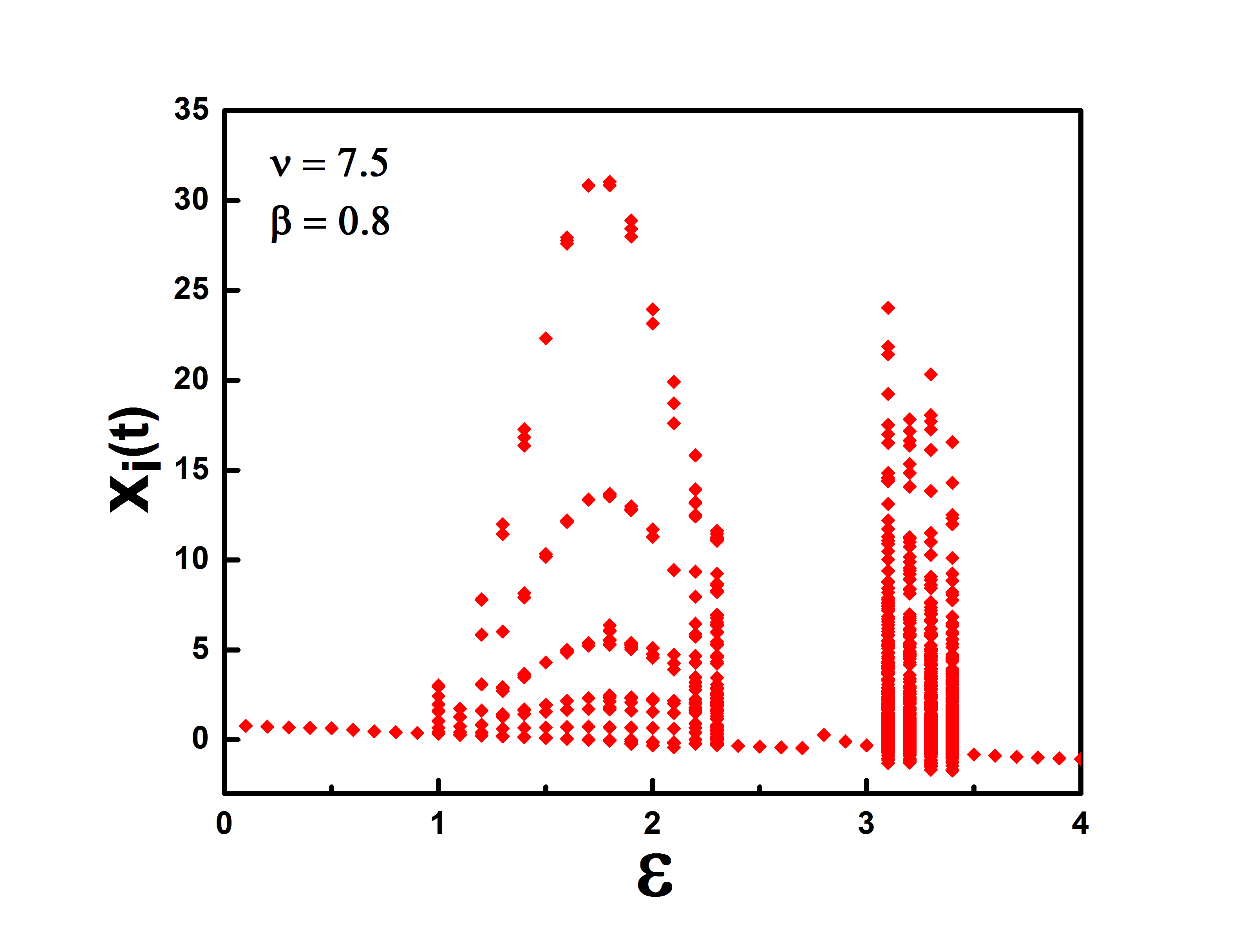
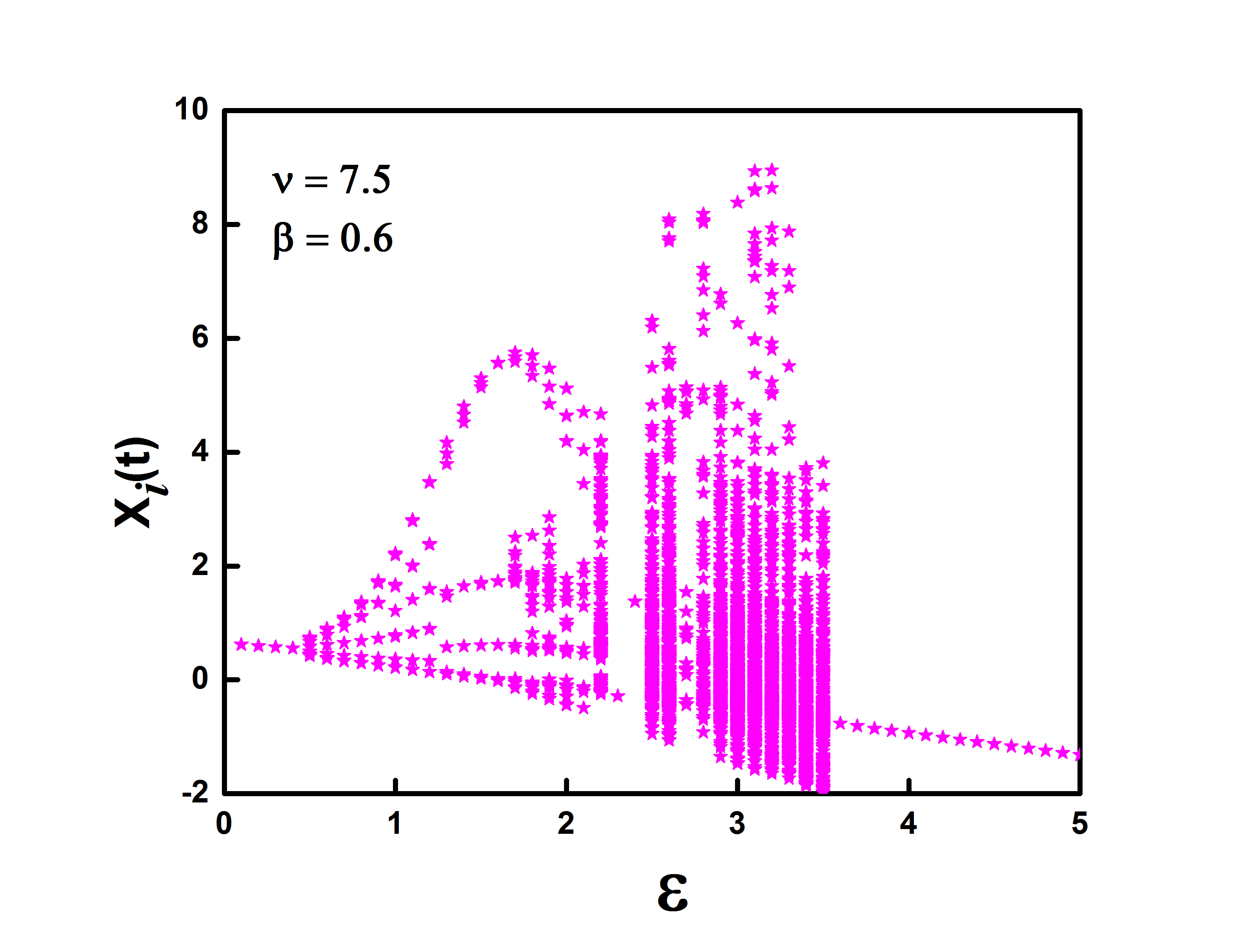
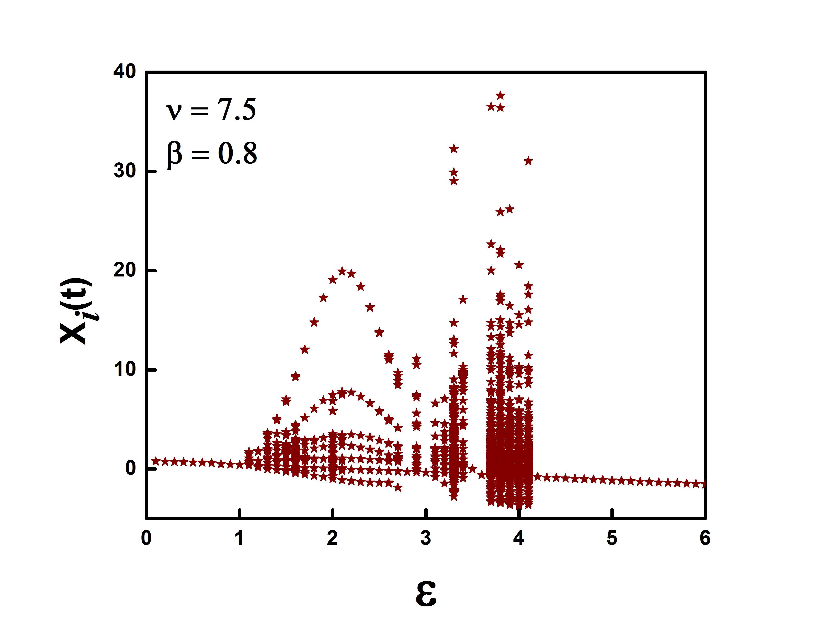
First, we study our model for a 5-site interaction coupled Gauss map. The bifurcation diagram is the most simple method for displaying dynamic behavior while varying a control parameter. We plot the bifurcation diagram for the 5-site coupled Gauss map for map parameters and [see Fig.2]. We consider and wait for . The bifurcation diagram displays the all values of sites as a function of coupling parameter at . The bifurcation plot shows a clear synchronization transition for a larger value of , which we investigate in detail.
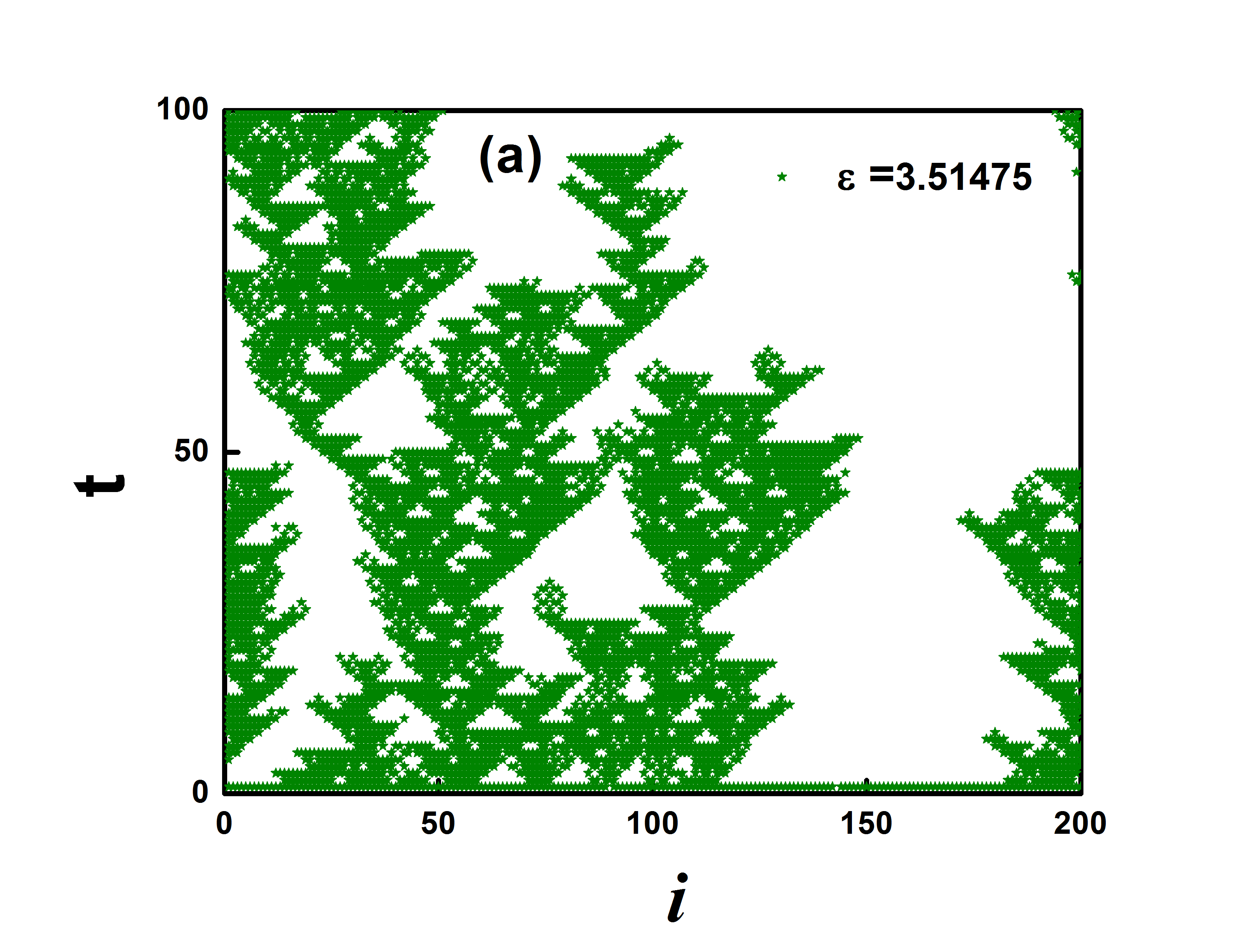
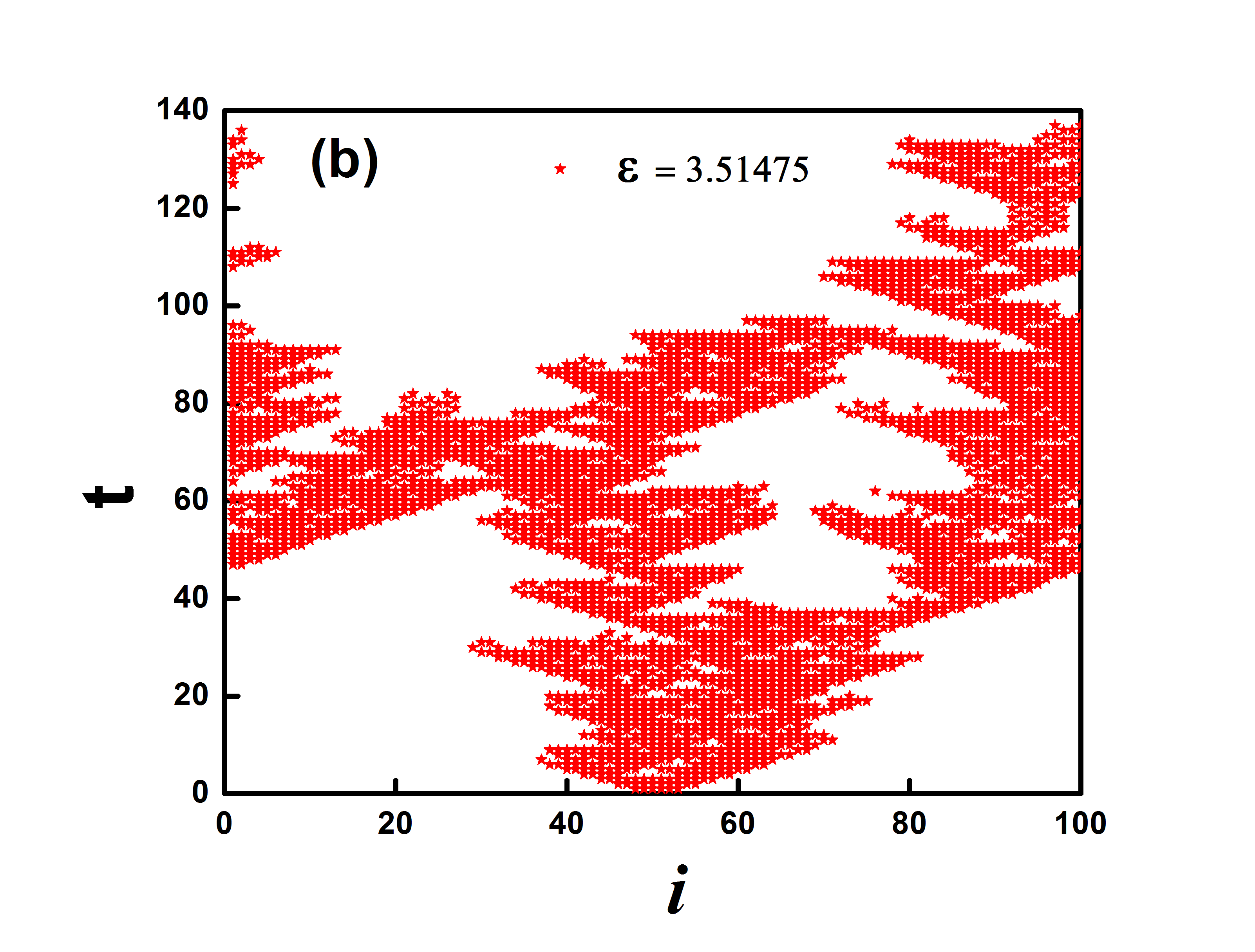
We also study the space-time diagram for visualizing the defects for the 5-site interaction coupled Gauss map. We plot it for discrete time as a function of site index (where ) for and . The behavior of such defects is plotted in Fig. 3 (a) and in Fig. 3 (b). (Defects are the sites for which where .) We observe the spatiotemporal intermittency (STI) in two different regions for both plots. There is no ‘solitonlike’ structure observed in this regime. A similar evolution is observed in janaki2003evidence for coupled map lattice defined in a standard manner (see Figure 1 and Figure 2 of janaki2003evidence ).
Saturation of persistence usually implies that the activity has stopped fully or partially. Hence the synchronization is accompanied by saturation of persistence. Thus, the order parameter becoming zero is accompanied by saturation of persistence. On the other hand, the active state will lead to persistence becoming zero if activity continues at all lattice sites. Thus, there is a critical value of coupling such that for the order parameter goes to zero and persistence saturates while for , the order parameter saturates and persistence goes to zero. For continuous transition, we observe power-law decay of both persistence and order parameter at the critical point . At such a critical point, the persistence and order parameter algebraically decays as:
| (6) |
| (7) |
The exponent is known as the persistence exponent and is the order parameter exponent. The exponents are not universal and depend on the details of the evolution of the system.
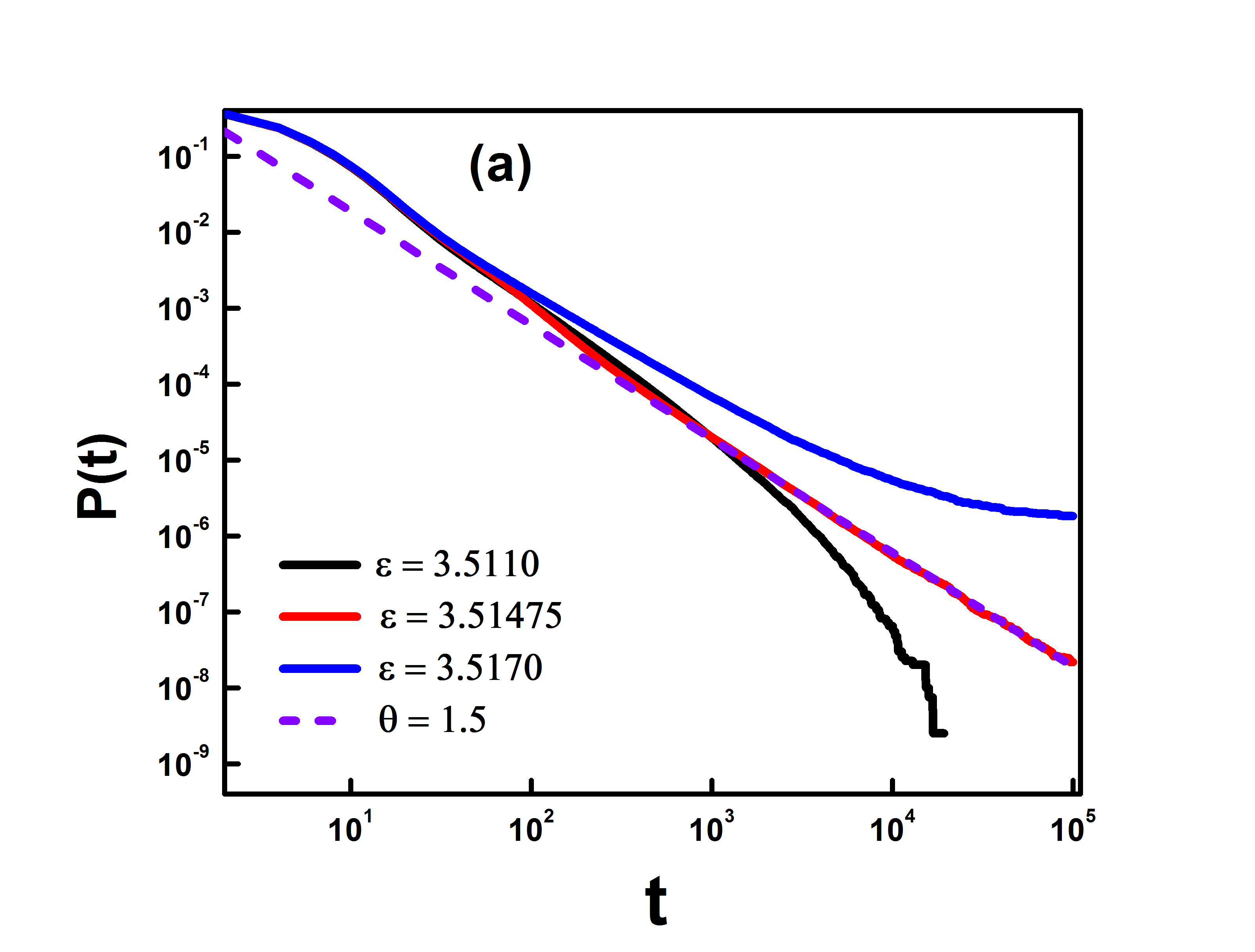
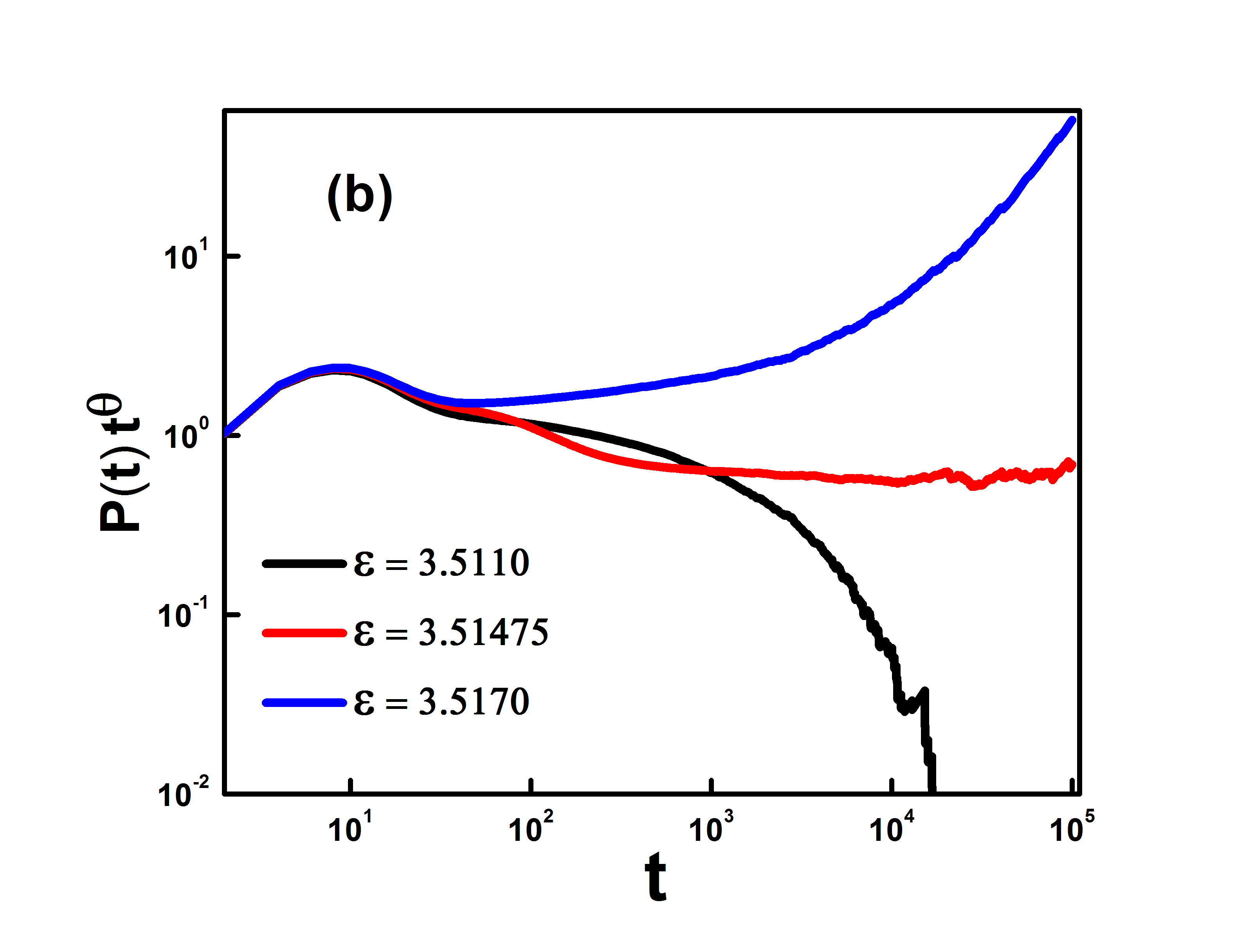
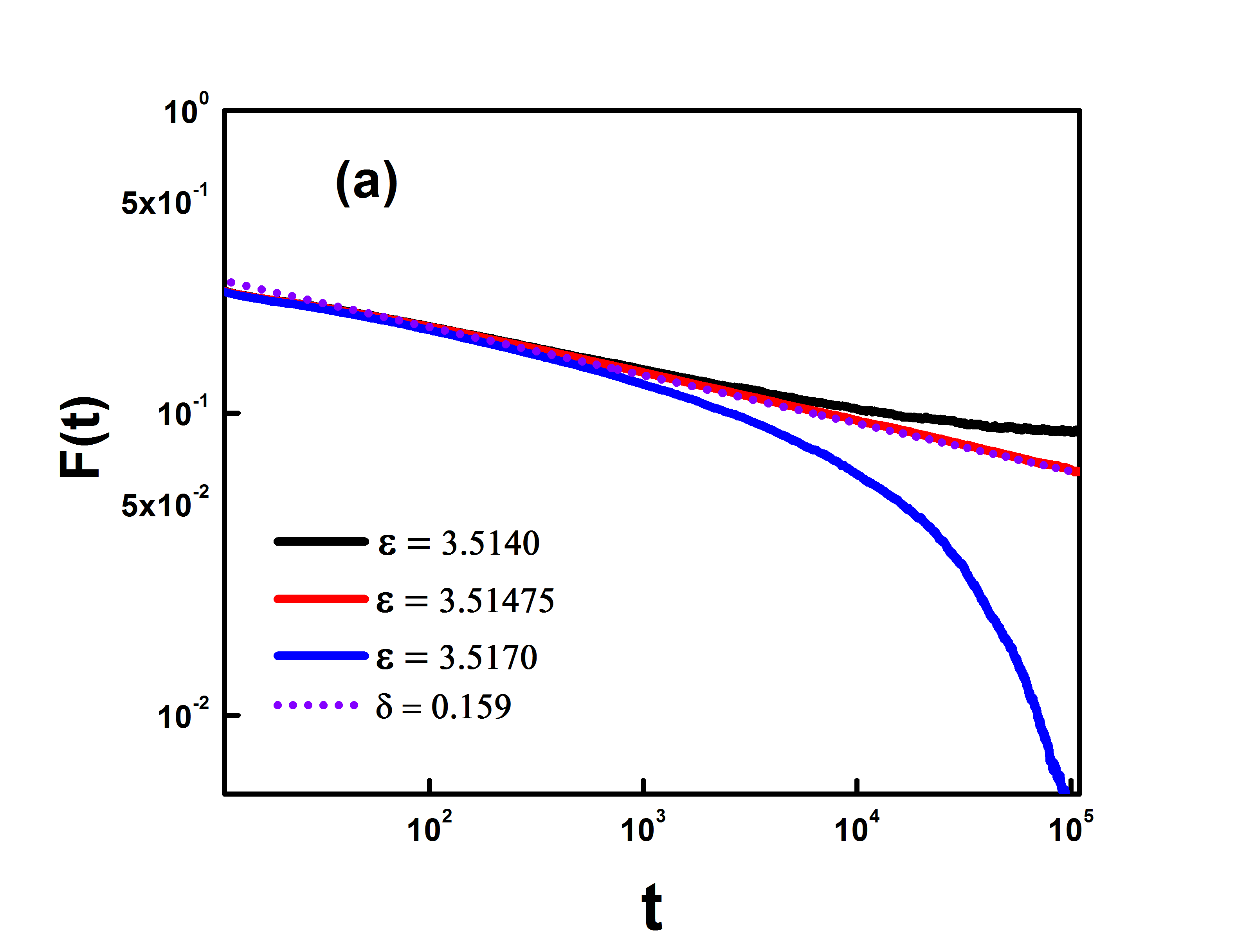
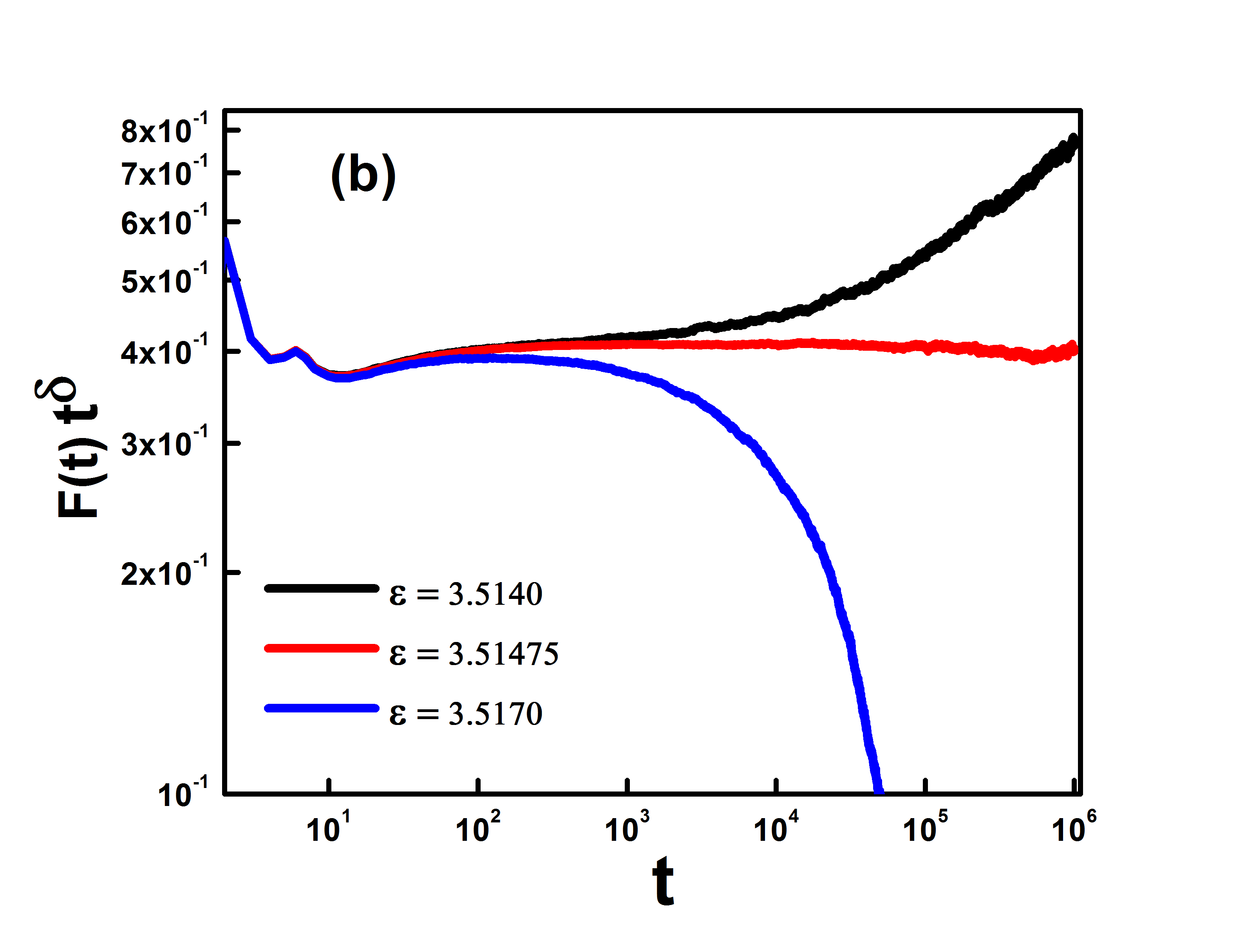
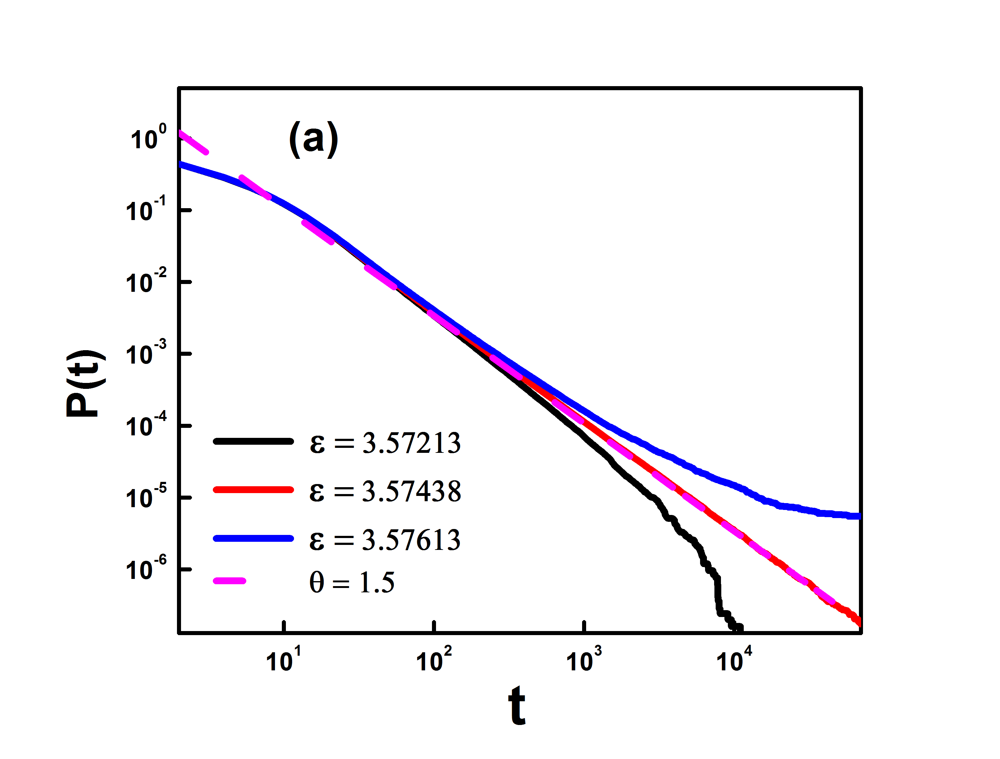
We simulate our 5-site interaction CML Gauss map for , , and . The initial conditions are random and we average over configurations. We plot both and as a function of time [see Fig. 4 (a) and Fig. 5 (a)]. From these plots, it can be seen that for , saturates and the decays exponentially as expected. Similarly, for , saturates and decays exponentially. At critical point , we observe and . The persistence decays with the exponent while flip rate decays with exponent . If and then and should be constant asymptotically. We plot and as a function of for , and at [see Fig. 4 (b) and Fig. 5 (b) ]. We find that both the quantity tends to a constant for as . For , the curve displays upward or downward curvature. This is alternative evidence for the confirmation of the obtained values of the exponent. The exponent and match with DP exactly.
To confirm the nature of transition, we carry finite-size and off-critical scaling to compute the exponents and . This exercise is carried out for both order parameter as well as persistence . To compute dynamic exponent , we carry out finite-size scaling simulations for distinct lattice sizes at . To compute , we carry out off-critical scaling. For this, we simulate a very large size lattice for various values of both above and below . We consider a lattice of size large enough so that finite size corrections are not important.
The scaling law for and hold to expect following relations:
| (8) |
| (9) |
where and are scaling function and departure from critical point.
Thus for , i.e. , we obtain
| (10) |
| (11) |
and as , we obtain
| (12) |
| (13) |
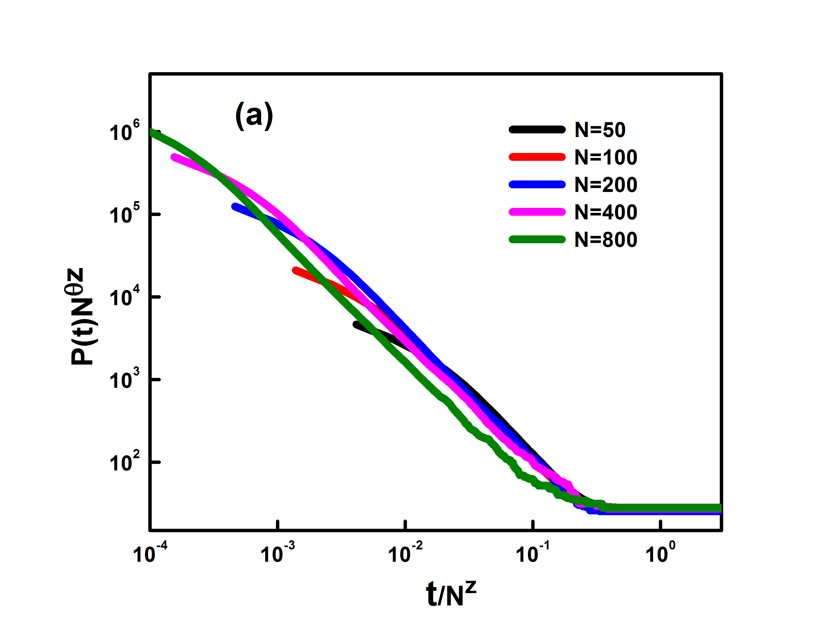
We simulate the lattice for , and and average over more than configurations. We plot as a function of at critical point and the good scaling collapse is obtained at which is shown in Fig. 6 (a). Similarly, we also plot as a function of and the fine collapse is obtained at [see Fig. 6 (b)]. The obtained values of dynamic exponent for both and exactly match the dynamic exponent of the DP class.
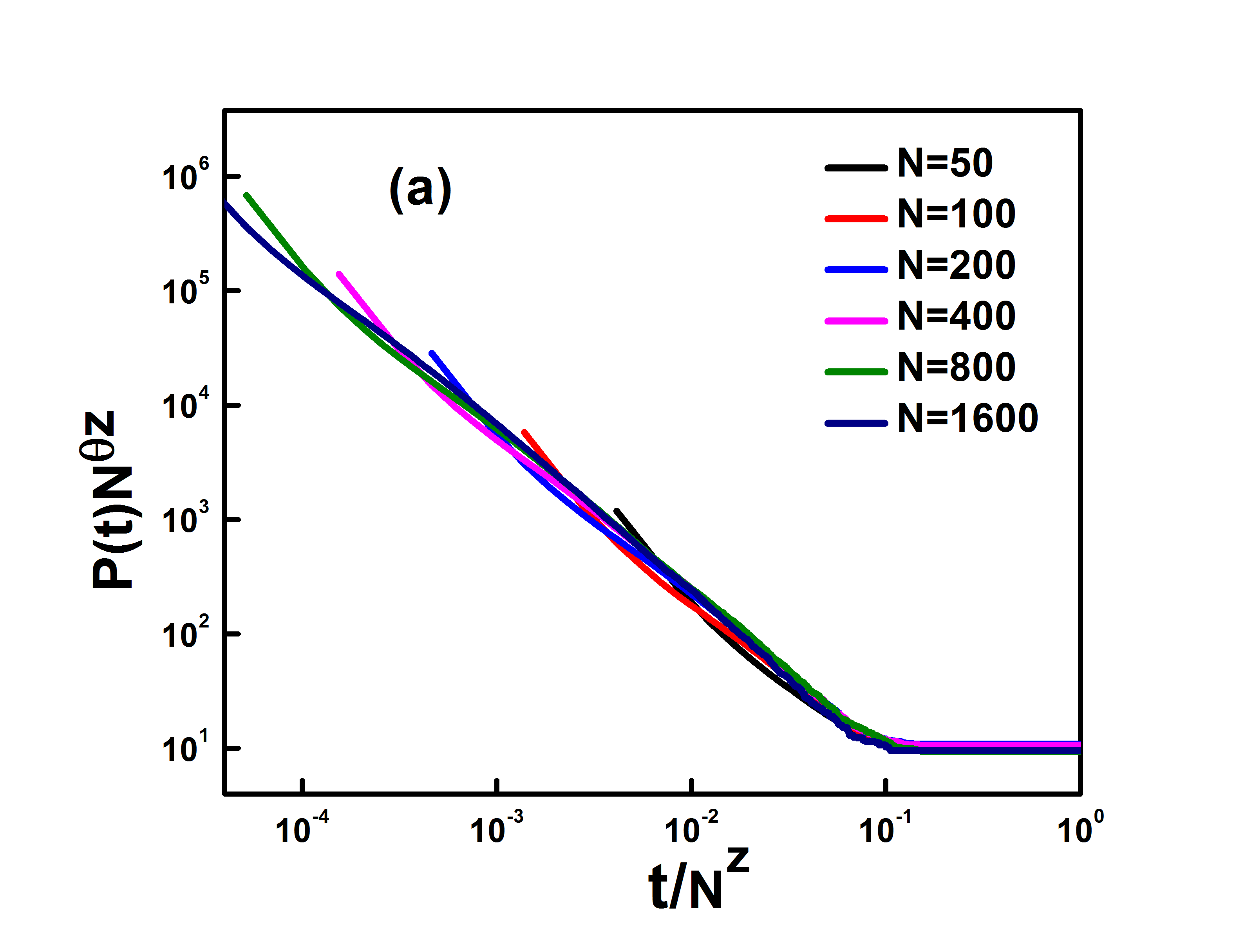
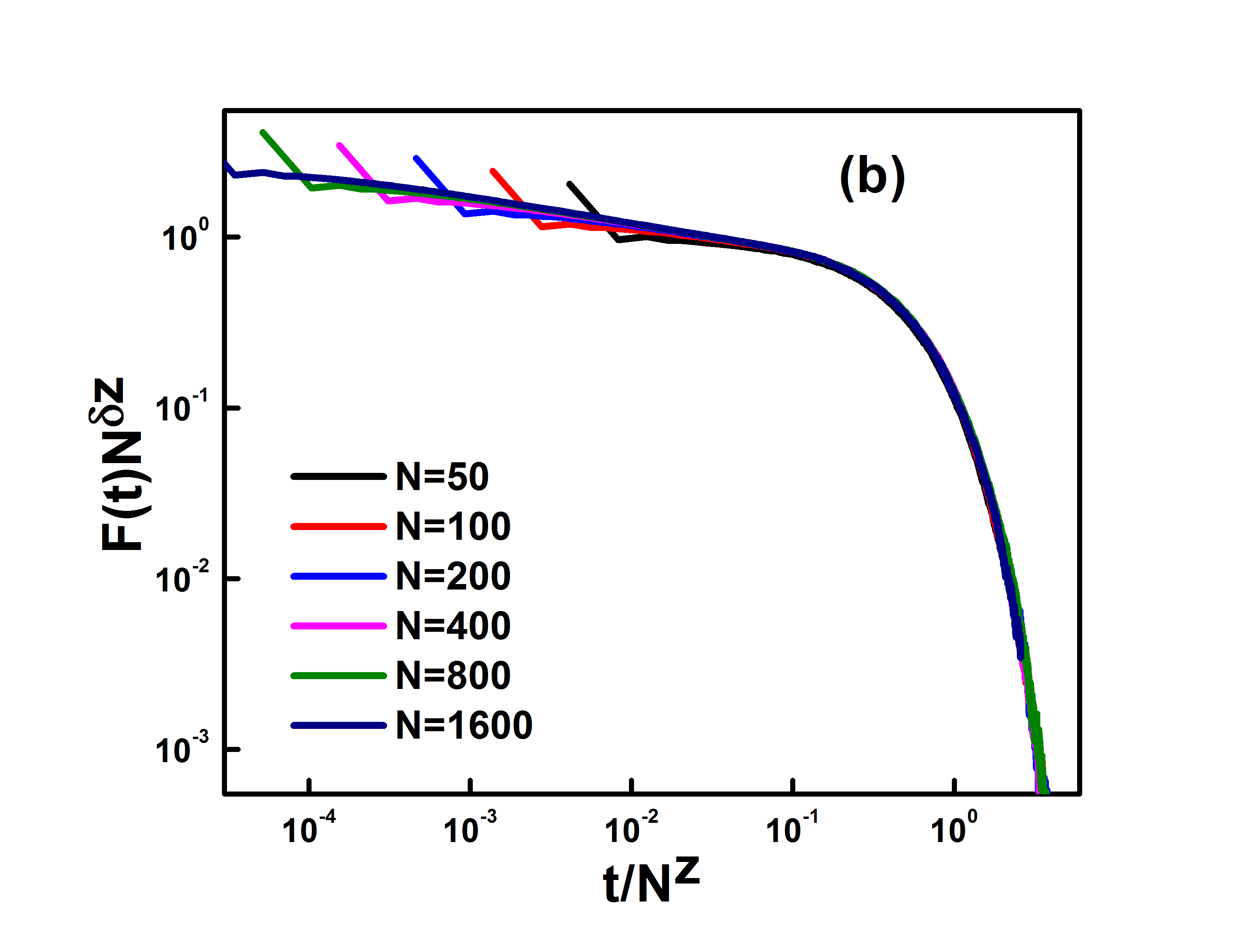
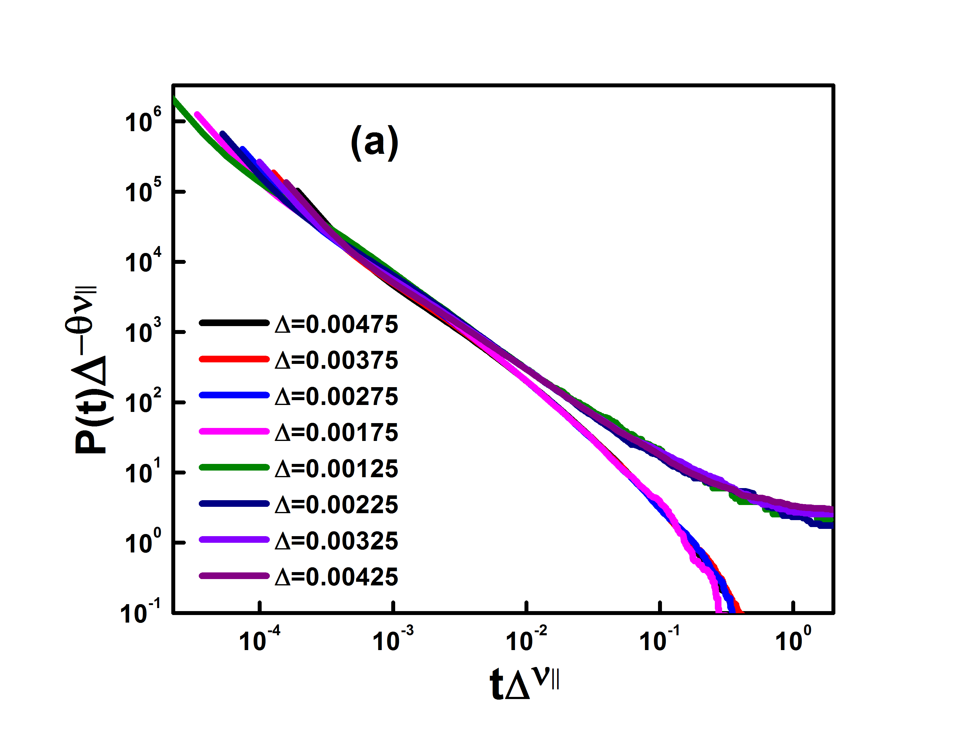
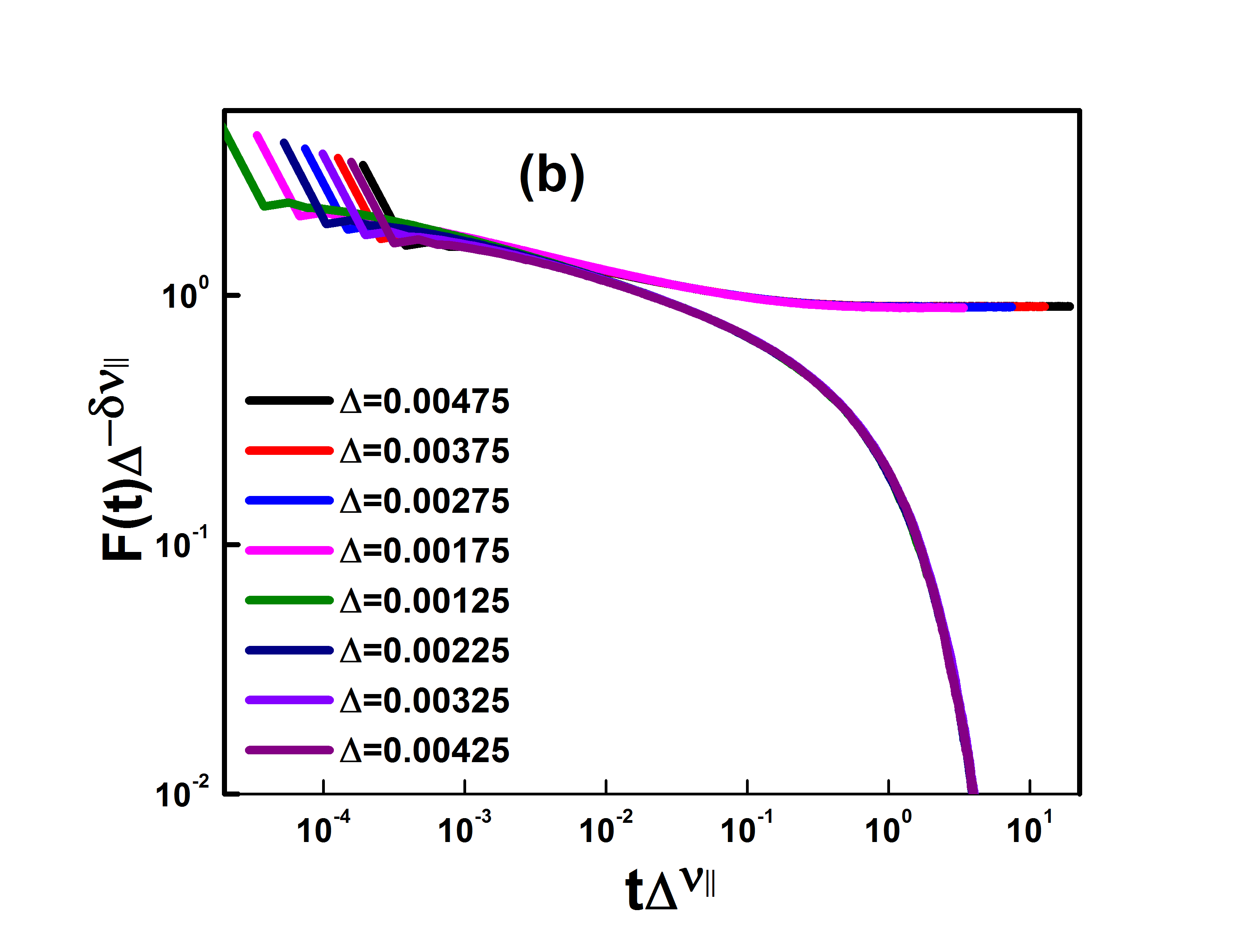
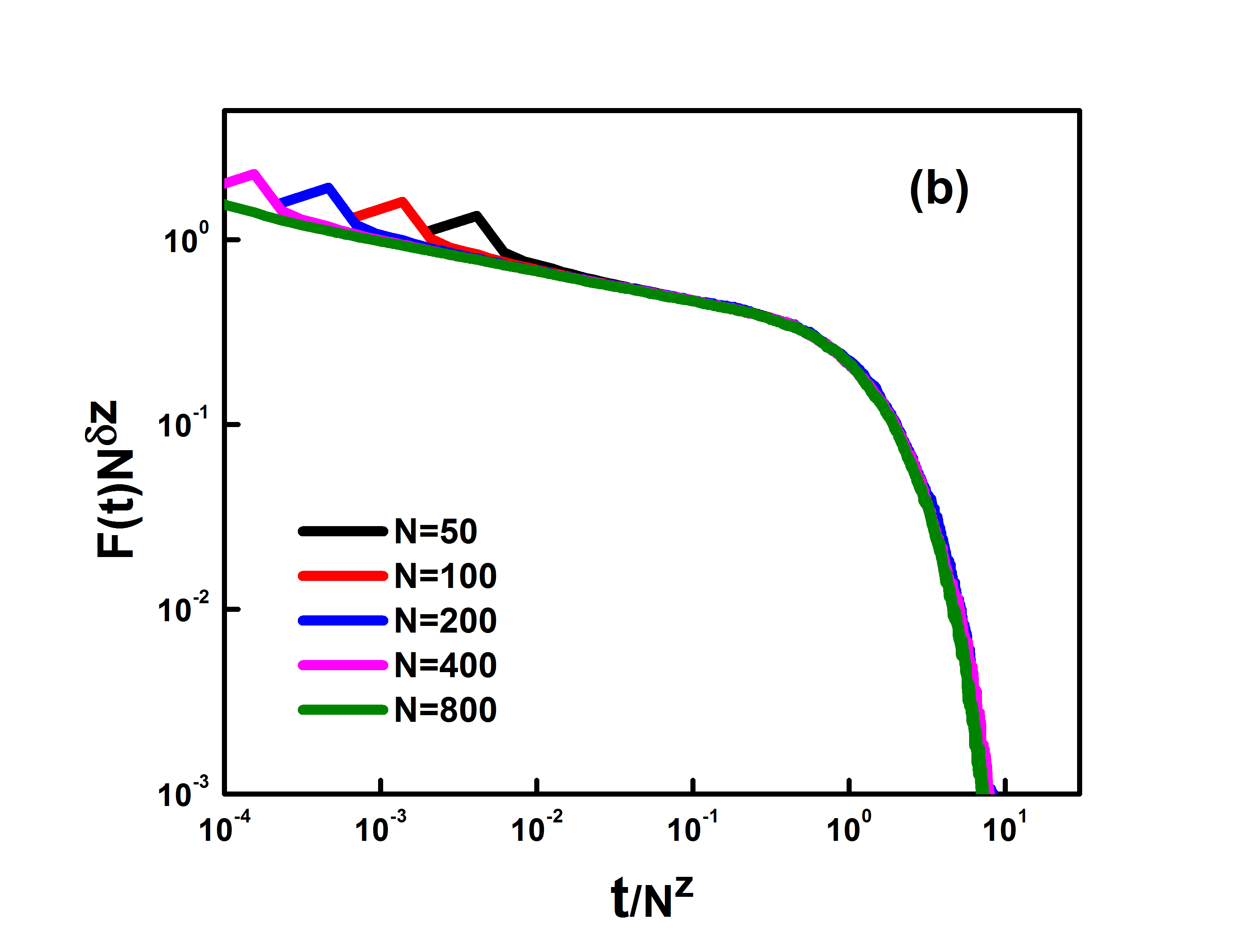
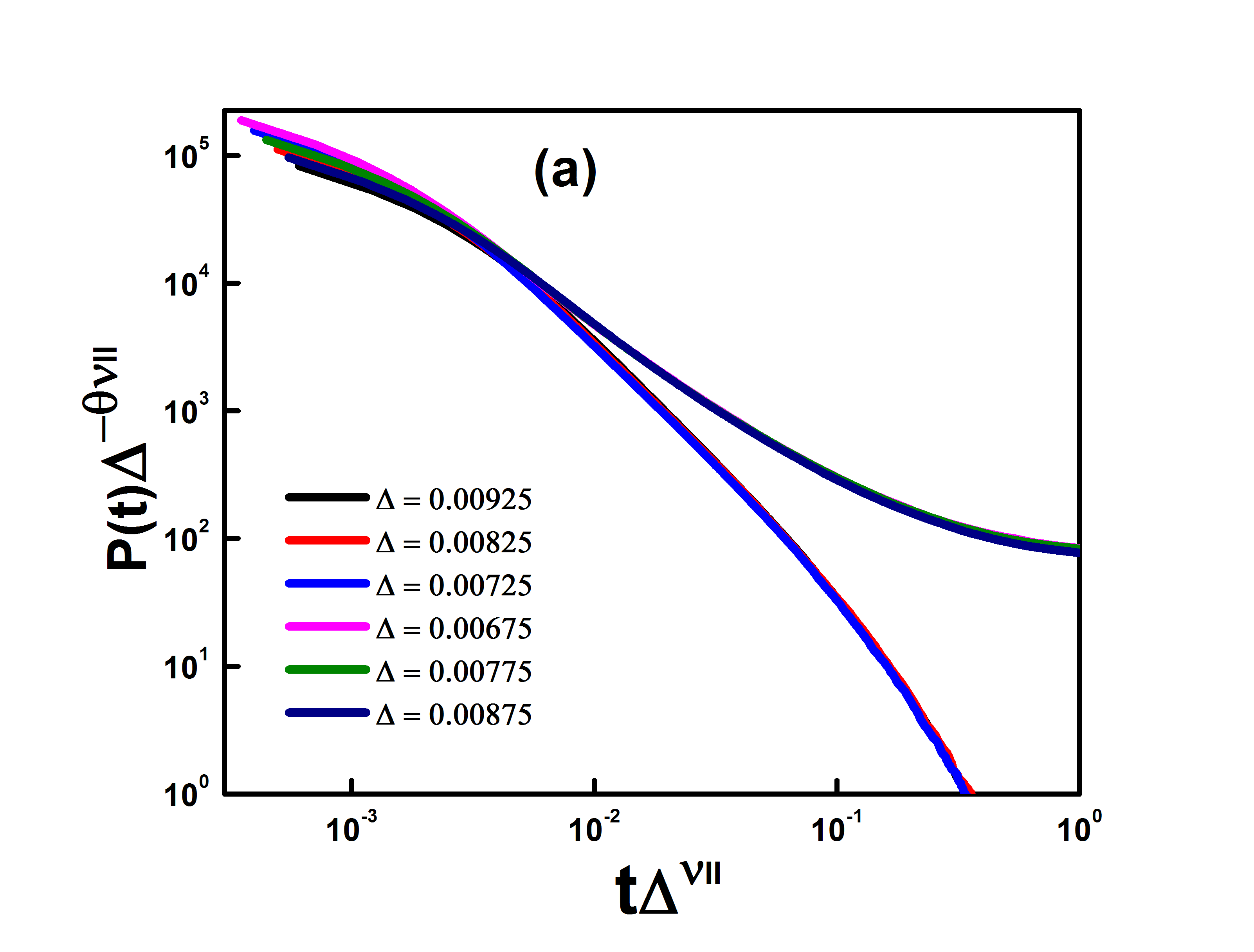
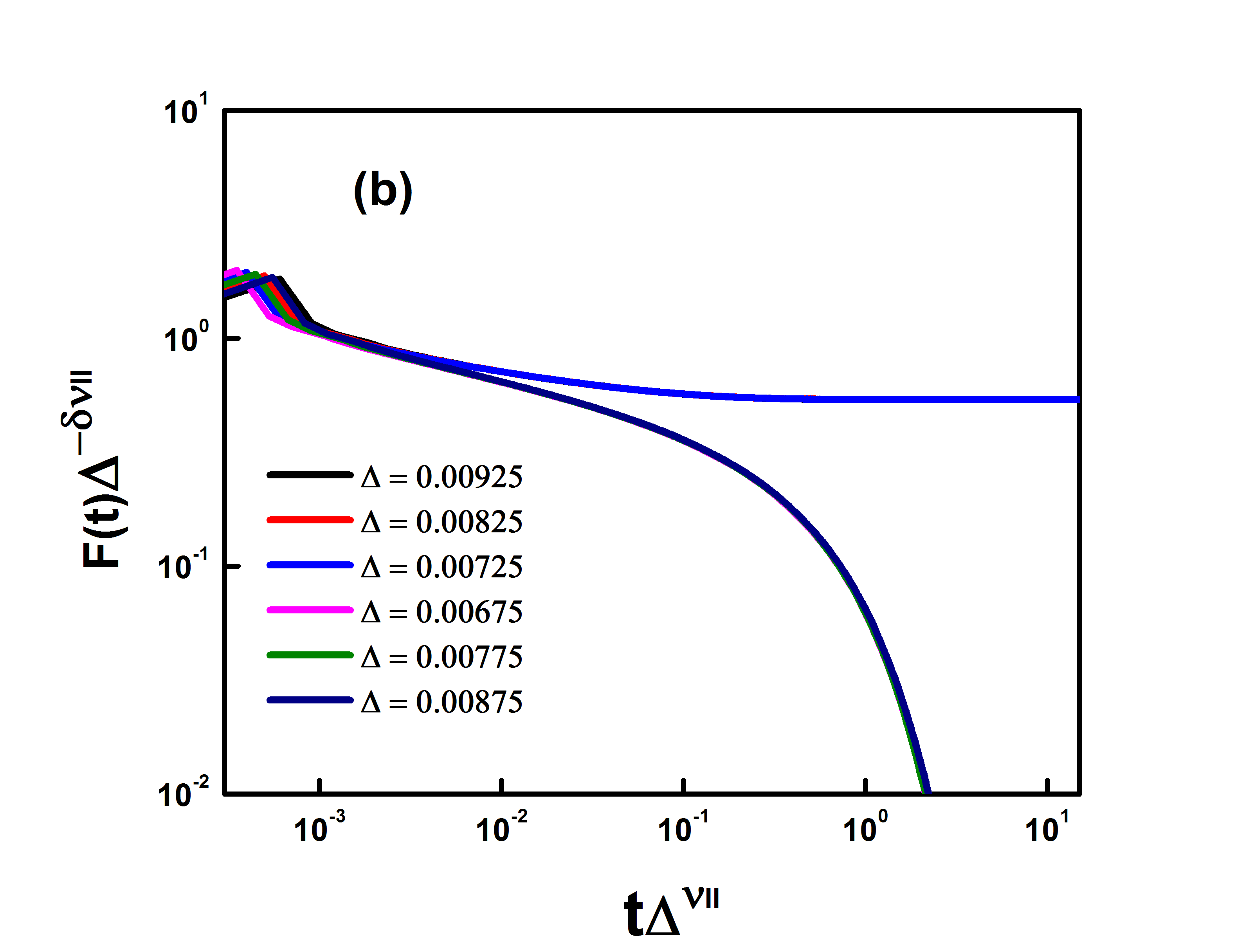
We note that for , decays to zero exponentially and saturates. For , decays to zero and saturates. We simulate a large lattice of size and average over more than 800 configurations for several values of above and below . We plot as a function of and the good scaling collapse is obtained for . This behavior is shown in Fig. 7 (a). Similarly, we plot as a function of and a good scaling collapse is obtained at . This collapse is shown in Fig. 7 (b). The obtained values of match with the exponent of the DP class exactly.
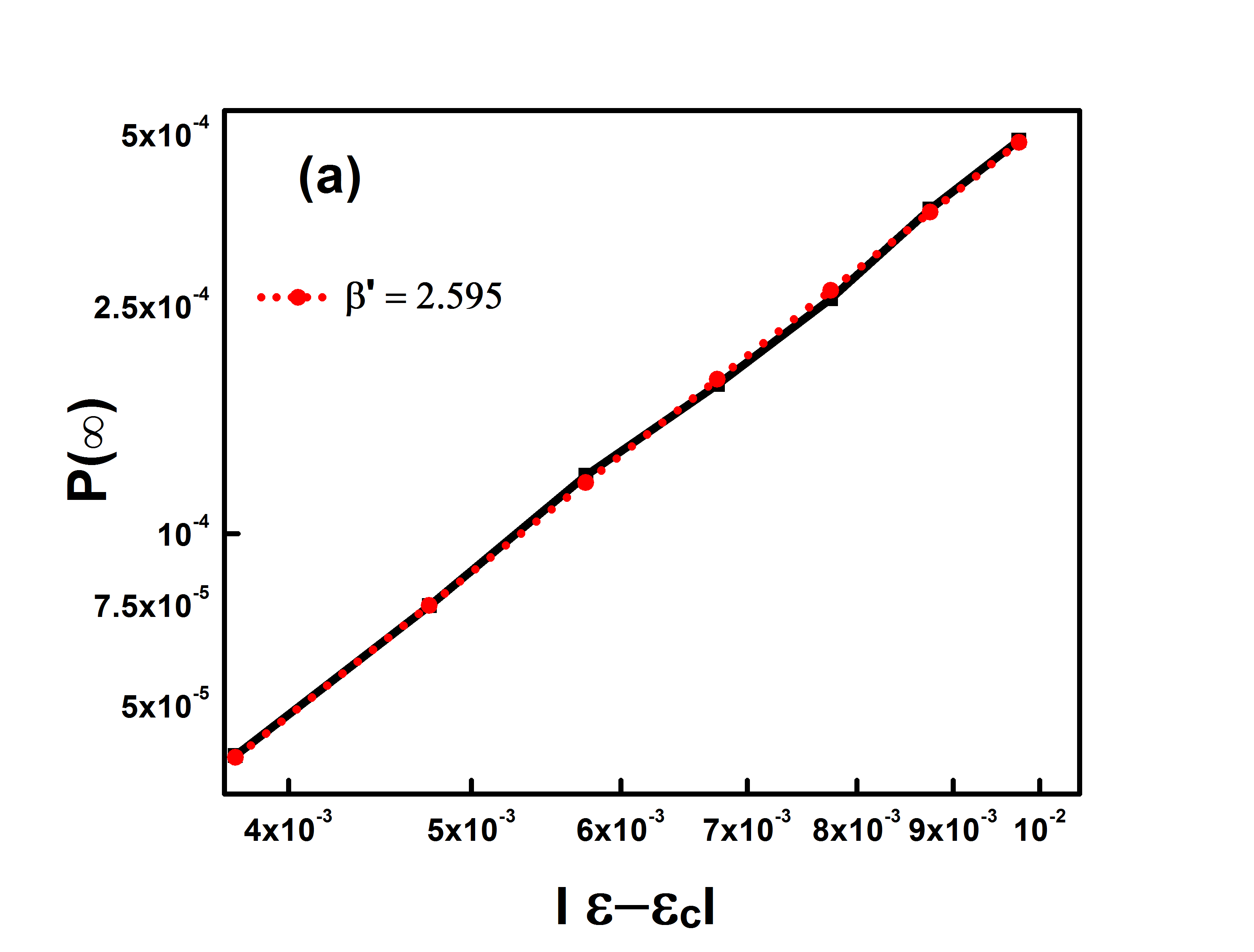
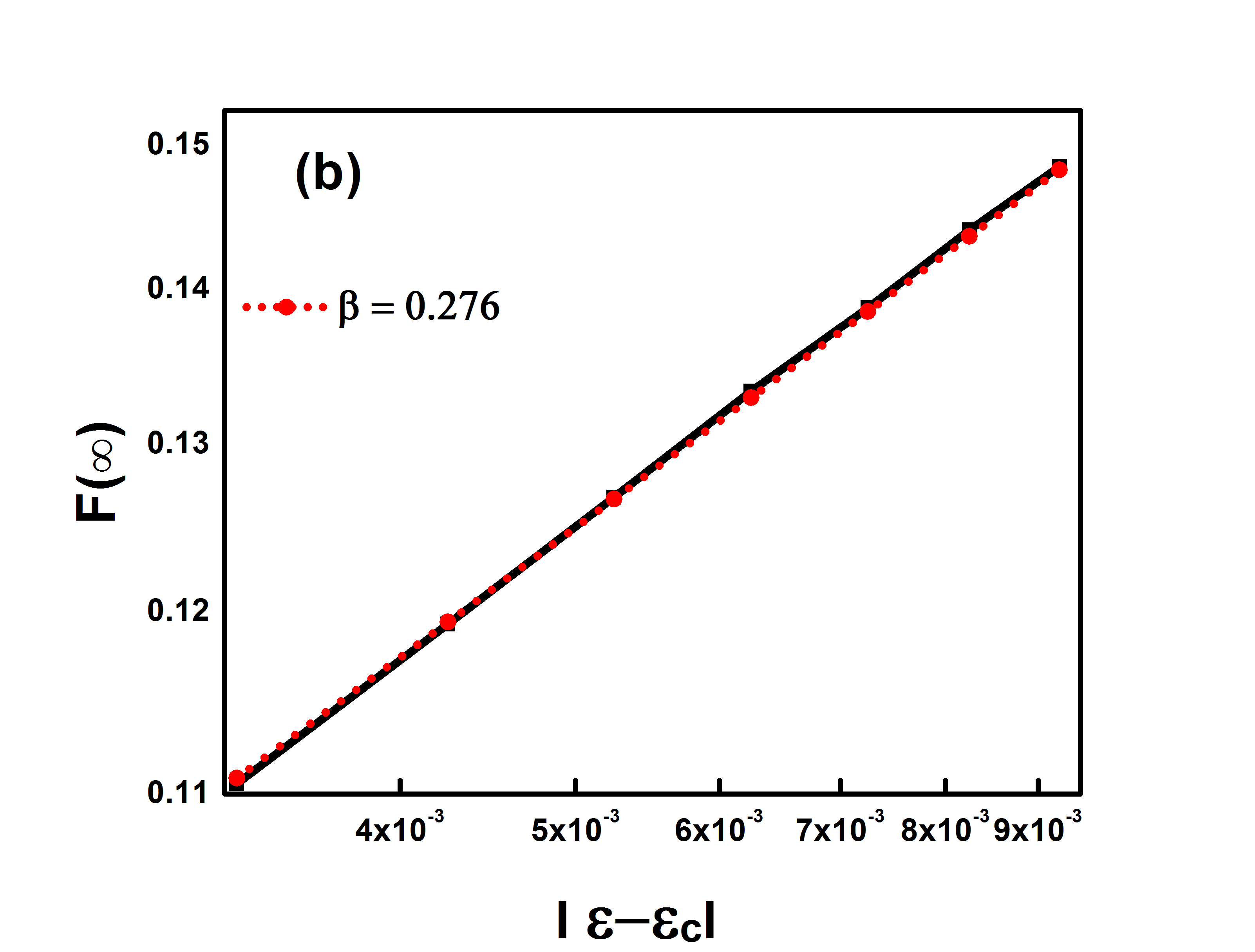
We expect the flip rate scale as , where = and = . Similarly, the persistence , where = and = . We consider and average over a configurations for both and . We plot = versus in Fig. 8 (a). The exponent . Similarly, we plot = versus in Fig. 8 (b). The exponent is found to be . These exponents are close to the expected value. They confirm the expected value of
3.2 Coupled map lattice with 3-site interaction
We also explore coupled Gauss maps with three-site interactions. We choose the map parameters of the Gauss map , , and plot the bifurcation diagram. We consider a lattice size of and wait for time steps. The resulting bifurcation plot displays all values of sites as a function of coupling strength . We plot the bifurcation diagram in Fig. 9. We observe the series of transitions from a fully synchronized state to a chaotic state by varying a coupling parameter. For larger values of , the system again displays a fully synchronized state.
To study the nature of phase transition for and , we simulate the quantifiers and for distinct values of the coupling parameter . We consider and average over configurations. We plot as a function of time steps in Fig.10 (a) and as a function of time steps in Fig. 11 (a). From this plot, we find that, with and with at critical point . The obtained exponents exactly match with exponents of the DP class. We have shown versus and versus for , and at in Fig. 10 (b) and Fig. 11 (b). We observe that the quantity and tends to a constant for as . For , the curve displays upward or downward curvature. This is alternative evidence for the confirmation of the obtained values of the exponent. The exponent and match with DP exactly. The multi-site interactions can also be termed as simplicial couplings.
Further, we study the finite-size scaling to compute the dynamic exponent . We consider lattice sizes and average over more than configurations for both and . We plot versus in Fig. 12 (a) and as a function of in Fig. 12 (b) at . From this plot, we observe that for a good scaling collapse is observed for and . While for a good scaling collapse is observed for and . The exponent obtained from finite size scaling for both and is exactly the same as the exponent of the DP universality class.
We study off-critical scaling to compute the exponent . We simulate the lattice for distinct values of for above and below the critical point. We consider and average over a configuration. We plot as a function of and the good scaling collapse is obtained for . This behavior is shown in Fig. 13 (a). Similarly, we plot as a function of and a good scaling collapse is obtained at . This collapse is shown in Fig. 13 (b). The obtained values of match with the exponent of the DP class exactly.
We expect the flip rate scale as , where = and = . Similarly, the persistence , where = and = . We consider and average over a configurations for both and . We plot versus = in Fig. 14 (a) and the exponent is found to be . Similarly, we plot versus = in Fig. 14 (b) and the exponent is found to be . This is further confirmation of the exponent
3.3 Coupled map lattice with 4-site interaction
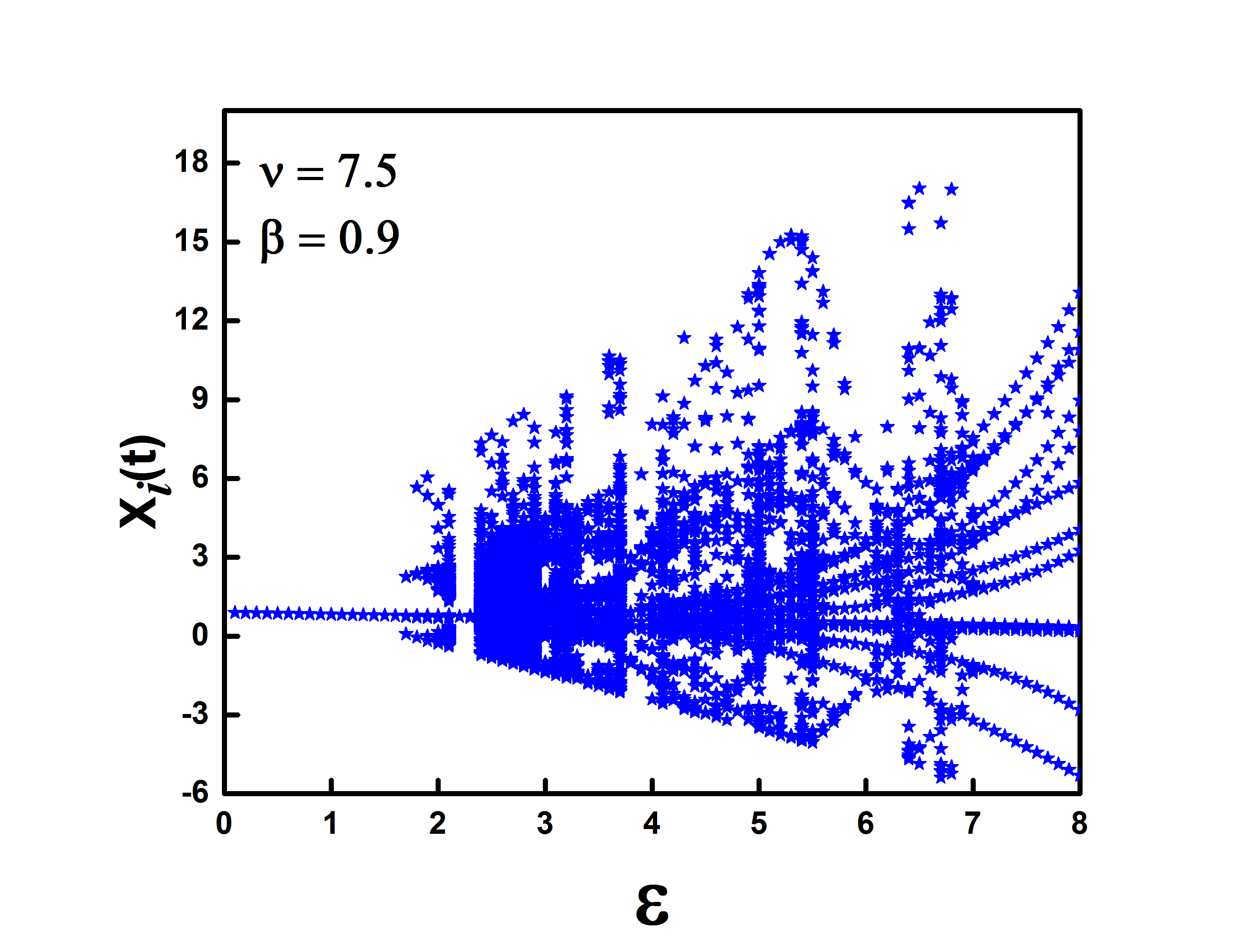
We also investigate the nature of the phase transition for even site interaction in a coupled Gauss map. We simulate our model for 4-site interaction. We choose the map parameters and and plot the bifurcation diagram for after waiting for steps. We plot the bifurcation diagram in Fig. 15. The bifurcation diagram is useful for visualization of the behavior of the system as a function of the coupling parameter. The bifurcation diagram captures the transition from a fully synchronized state to chaos. As the coupling parameter is increased further, the system reaches a synchronized state. We focus on one of the transitions to synchronization that shows continuous transition.
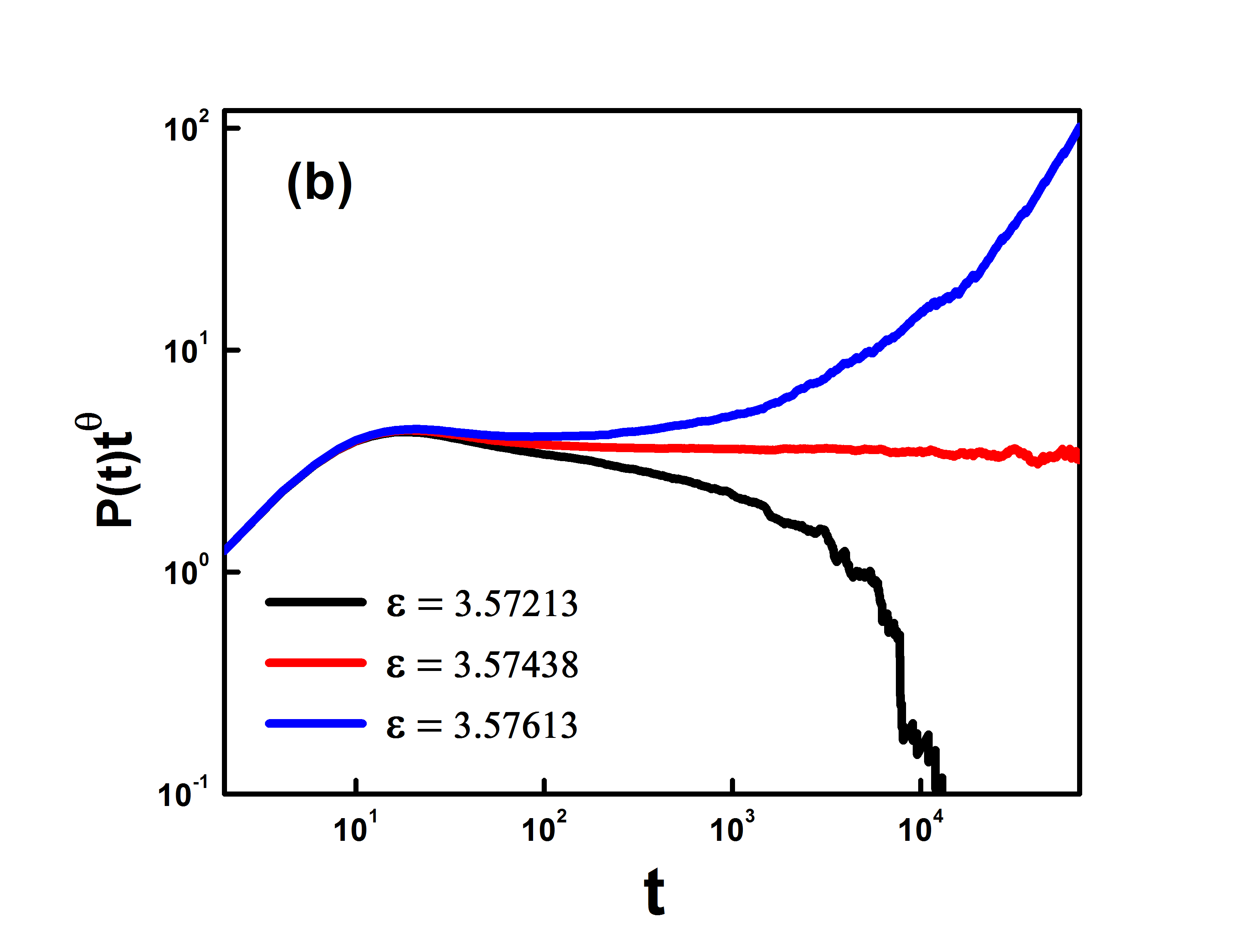
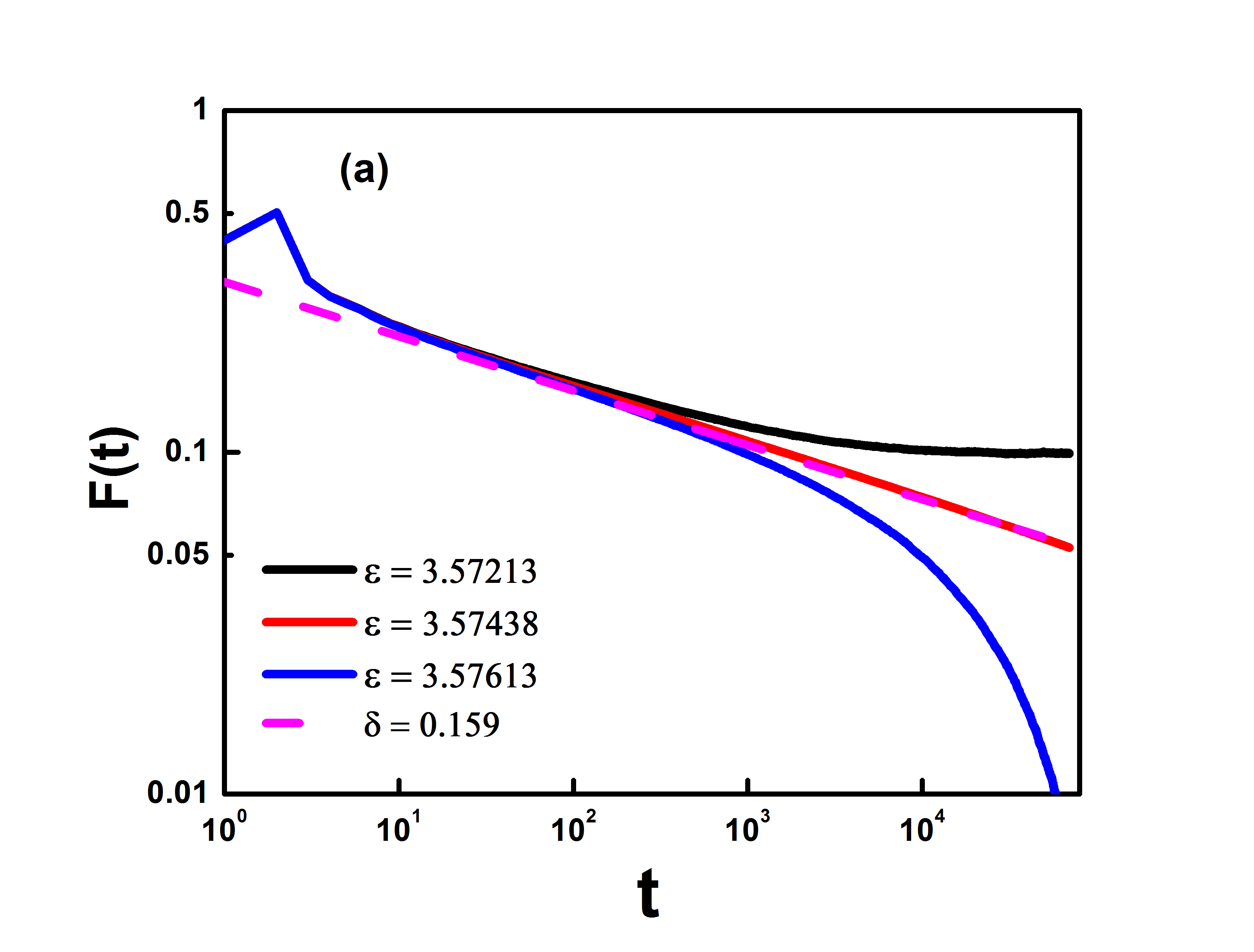
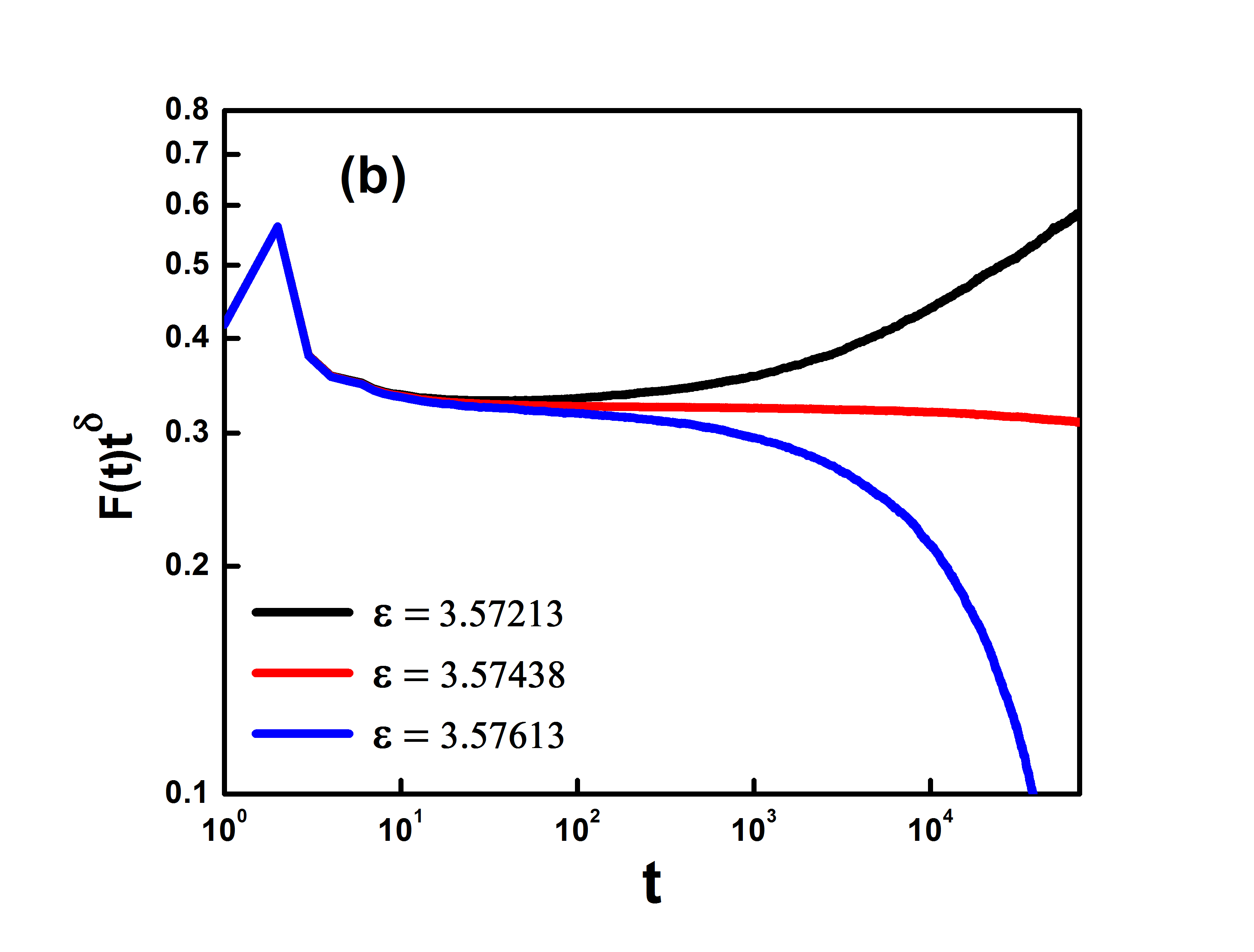
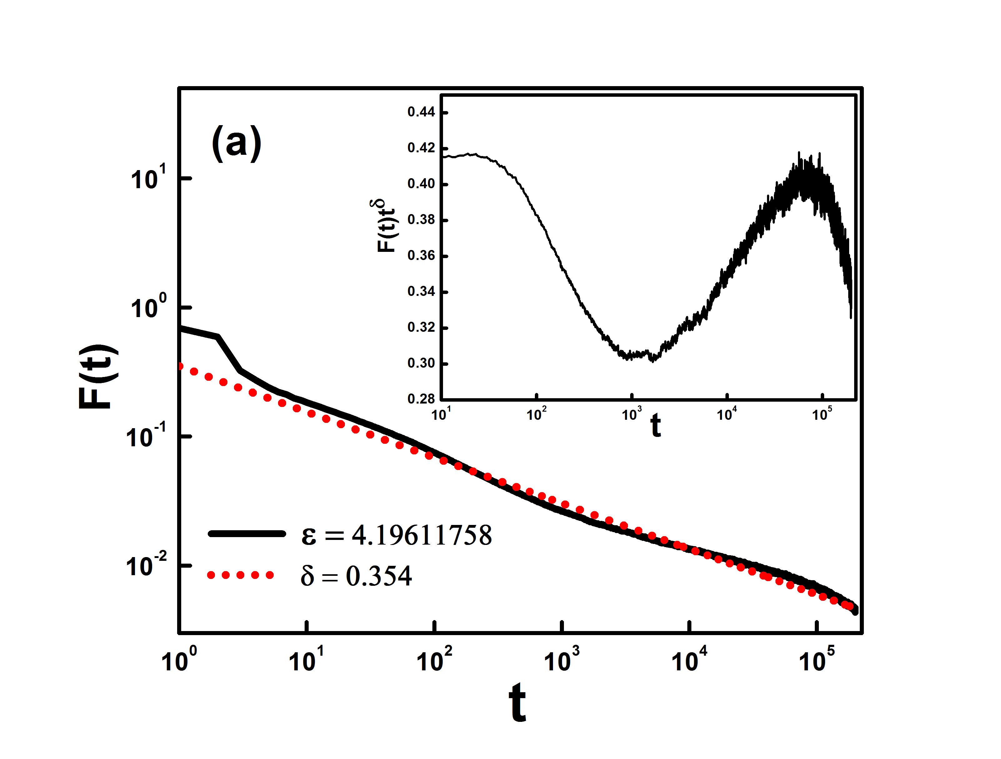
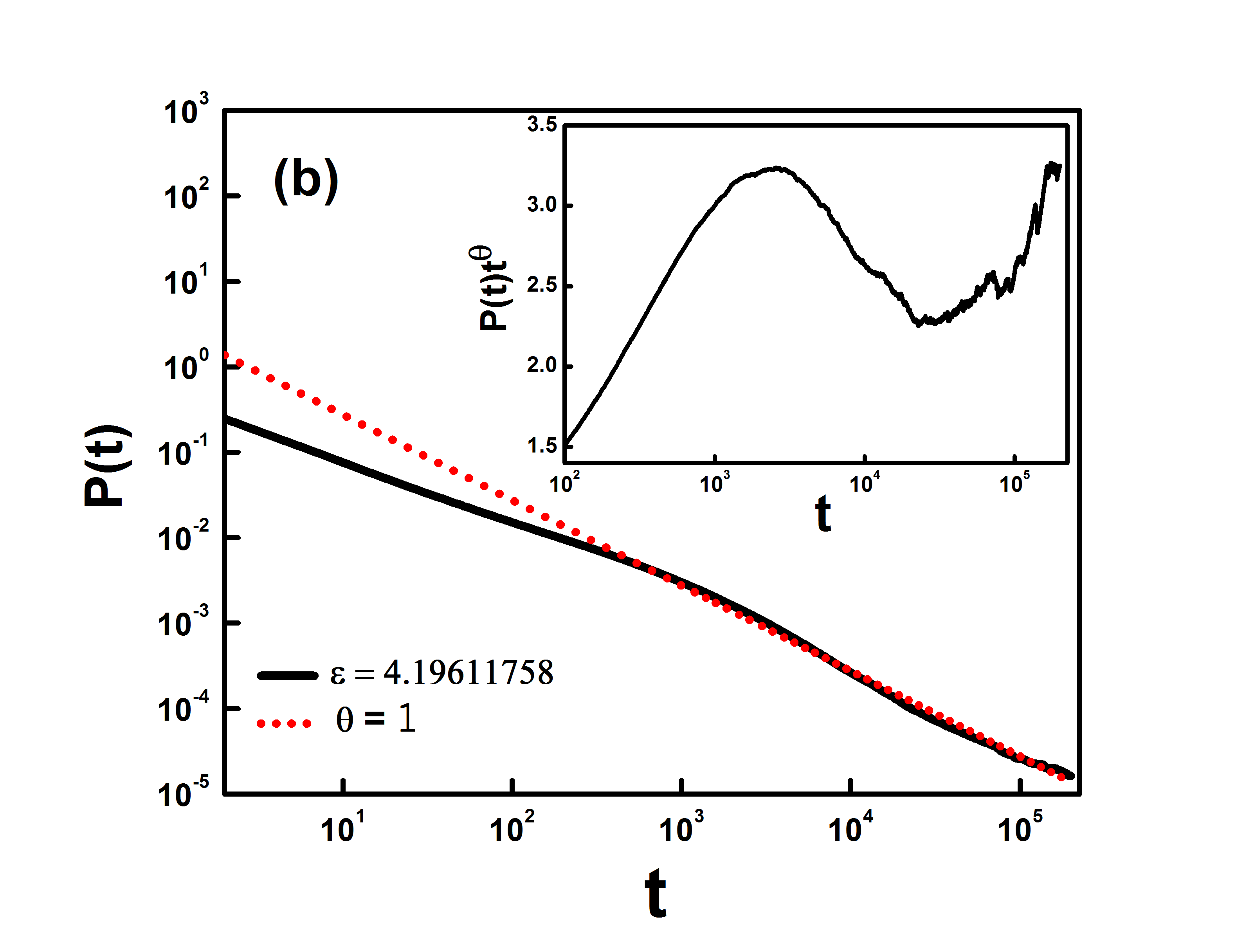
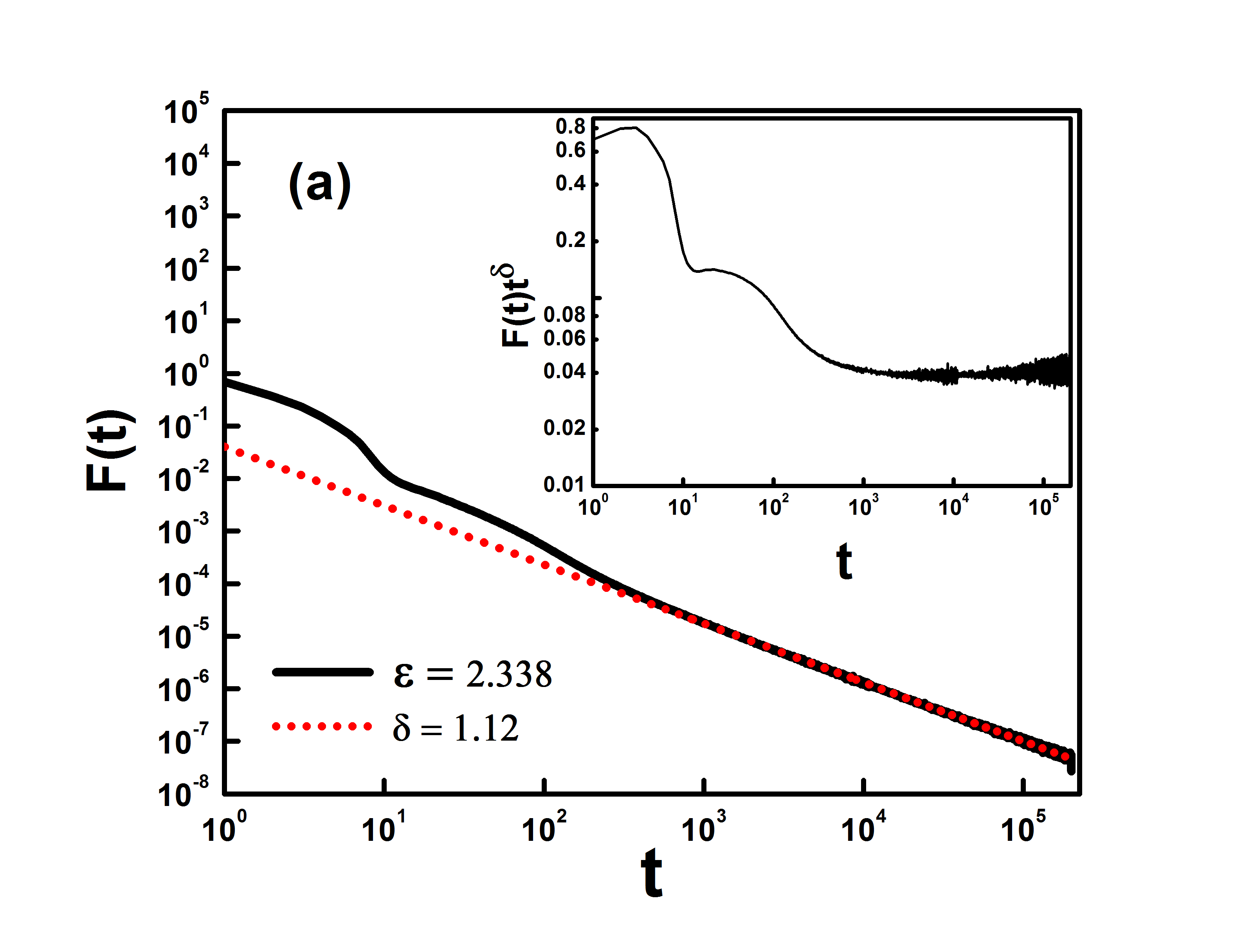
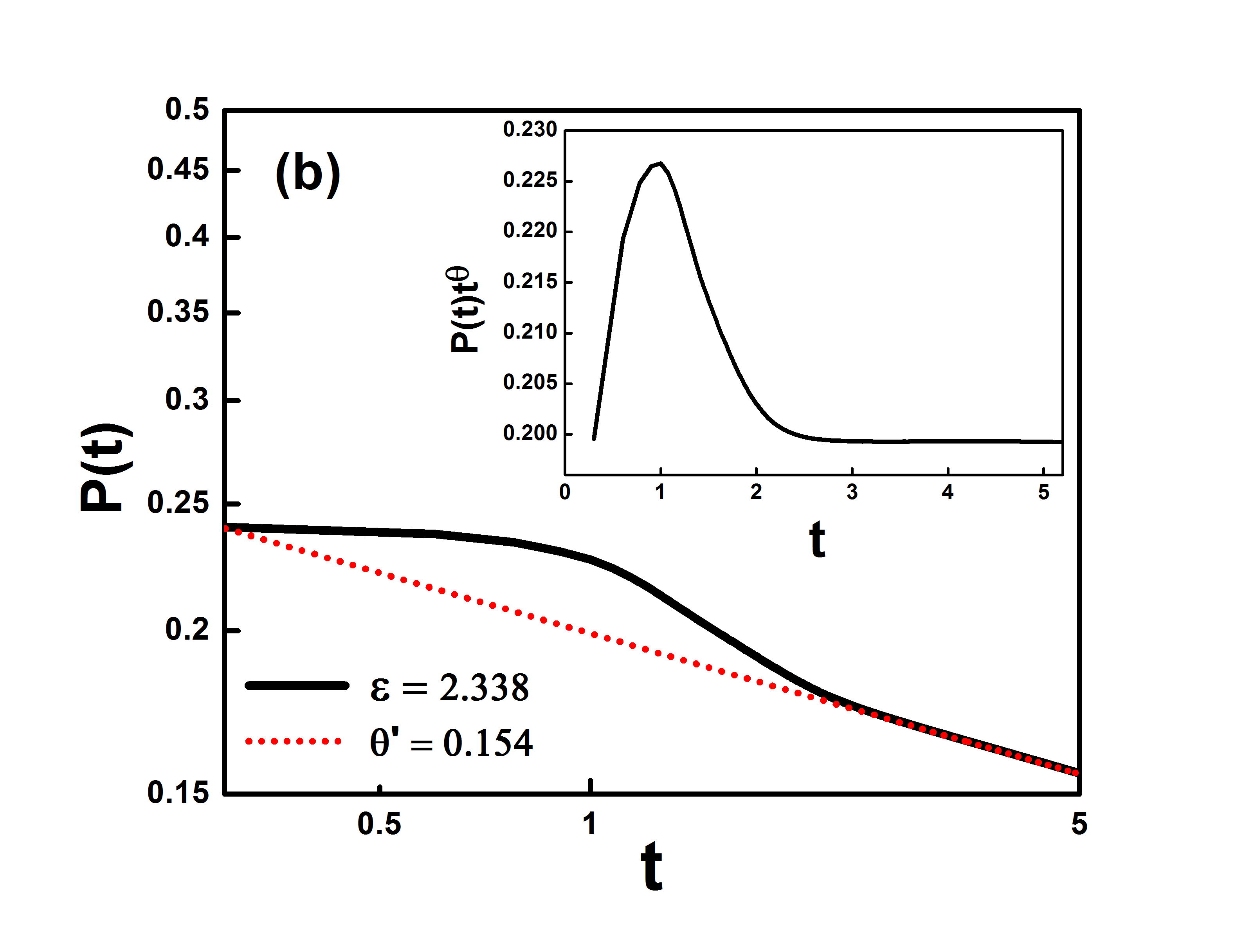
We compute the flip rate and persistence as the order parameter at the transition point for this system. We consider and average over a configuration. We plot as a function of time steps in Fig. 16 (a). We observe that shows power-law decay with logarithmic oscillation at . The decay exponent is found to be . We have displayed the as a function of for the same data in the inset plot. This plot confirms a clear oscillation over and above the power-law. Similarly, we plot as a function of time in Fig. 16 (b). We find that shows power-law decay superposed with logarithmic oscillations at . The decay exponent is found to be . We also plot as a function of for the same data in the inset plot. This plot displays oscillations over and above the power-law that confirm the values and logarithmic oscillation. This provides a novel transition with an exponent that does not match DP for both persistence exponent or . Therefore, the 4-site interaction is a relevant perturbation that emerges in a novel transition for the Gauss map.
3.4 Coupled map lattice with 2-site interaction
Lastly, we investigate the model with 2-site interaction. We consider , wait for , and plot the bifurcation diagram for and . The bifurcation diagram depicts the behavior of the system as a function of the coupling strength. Fig. 17 shows the bifurcation diagram. From this plot, we find that the system displays a fully synchronized state for low coupling. A transition occurs at = 1.5 and again for 2.1 2.4, and the system transitions to a synchronized state. We again investigate the point that shows a continuous transition.
We compute the flip rate and persistence for and average over a configuration. Fig. 18 (a) shows the plot as a function of time . The inset on the main figure shows the plot of as a function of . We find at . The decay exponent is found to be . This exponent is very different from the DP class. We also plot as a function of in Fig. 18 (b). It decays as The inset shows a plot of as a function of with . The persistence decays slower than power-law in this case and there is no well-defined persistence exponent.
Summary
Directed percolation is one of the most widely observed non-equilibrium dynamic transitions to an absorbing state. Of late, it has been observed in experimental situations as well. Most of these systems are modeled by equations involving a Laplacian. The standard formulation of coupled map lattices can be considered as discretized Lapcian. It involves pairwise interactions. This model is not a discretized Laplacian and the interactions are multi-body multiplicative interactions.
In this work, we study the coupled Gauss map for odd and even site interaction in one dimension. We study 3-site and 5-site for odd sites and 2-site and 4-site for even sites interaction. The coupling is such that it cannot be decomposed into pairwise interactions. We have classified the sites, considering fixed points as a reference. If the variable values are above or below the fixed point, then the associate spin is or . We investigate the phase transition using quantifiers such as the flip rate and persistence .
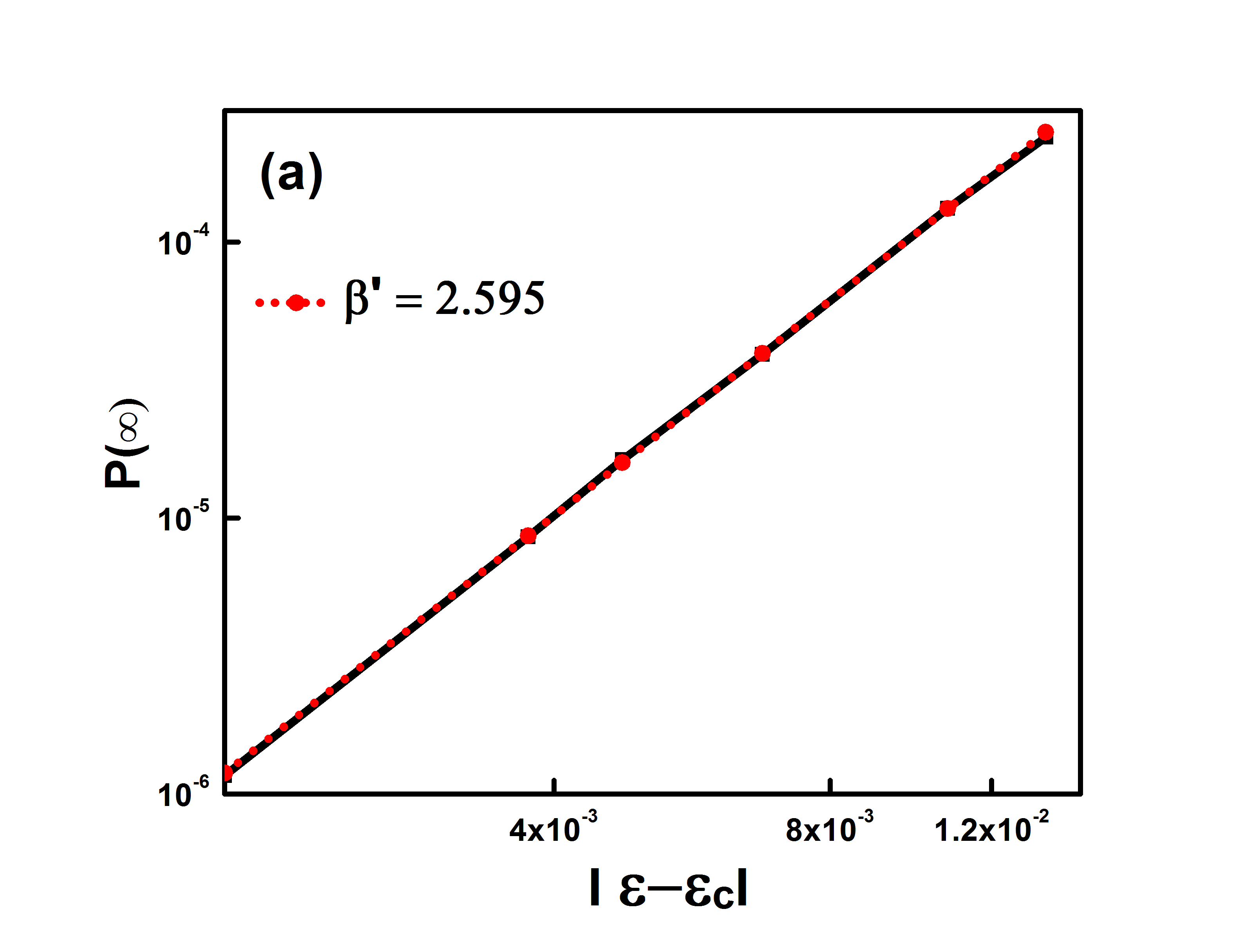
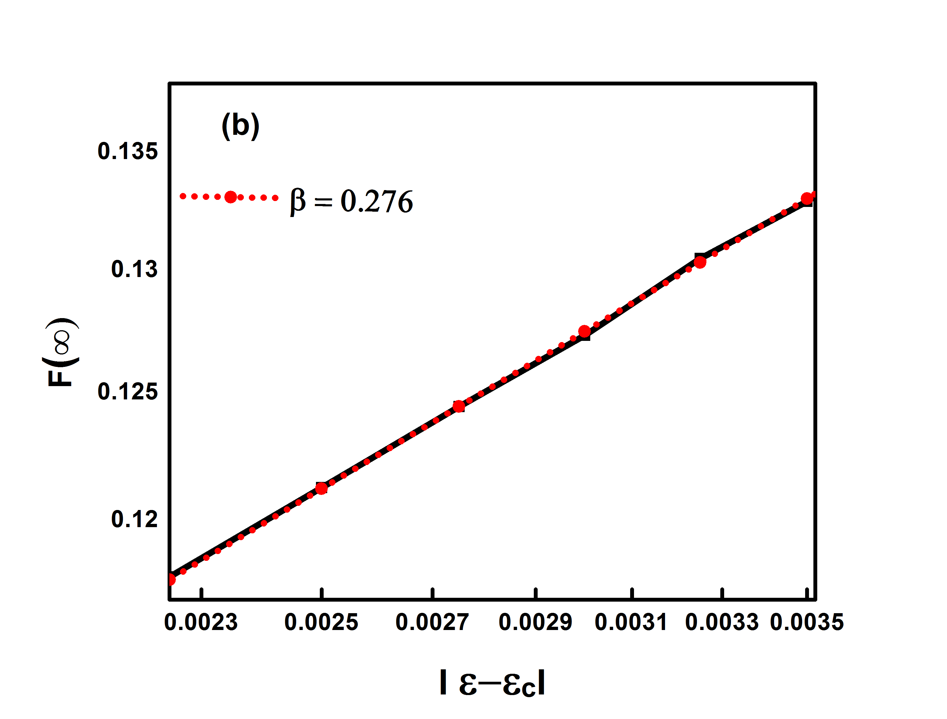
For 3-site and 5-site interaction, we find the power-law decay of flip rate and persistence at a critical point. The decay exponent for is =0.159 and for is =1.5. We also study the finite-size scaling and the off-critical scaling. The obtained exponents , , and =0.275 match exactly with the exponents of the DP universality class. Thus DP class is robust for 3-site and 5-site interaction studied in this work.
For even site interaction, the exponents change. For 4-site interaction, we find the decay exponent and . We observe the logarithmic oscillations over and above the power-law. For 2-site interaction, we find the decay exponent =1.12. The persistence decays slower than power-law as . The behaviors are different from DP and they are different from each other. Thus, multi-site couplings could lead to a new universality class. It could depend on the number of coupled sites. It could also depend on the detailed nature of the map. Further studies on different maps as well as interactions could be of interest. The results are quite surprising given the fact that only a few universality classes are known for absorbing state transitions.
Acknowledgments
PMG thanks DST-SERB (CRG/2020/003993) for financial assistance.
Author Contribution
MCW and PMG contributed to conceptualization, simulations, visualization, and drafting.
Statements and Declarations
The authors declare that they have no conflict of interest.
Data Availability Statement:
This manuscript has no associated data or the data will not be deposited. [Author’s comment: All data that support the plots within the paper and other findings of the study are available from the first author upon reasonable request.]
References
- [1] AV Andreev, NS Frolov, AN Pisarchik, and AE Hramov. Chimera state in complex networks of bistable hodgkin-huxley neurons. Phys. Rev. E, 100(2):022224, 2019.
- [2] Luciano da Fontoura Costa, Osvaldo N Oliveira Jr, Gonzalo Travieso, Francisco Aparecido Rodrigues, Paulino Ribeiro Villas Boas, Lucas Antiqueira, Matheus Palhares Viana, and Luis Enrique Correa Rocha. Analyzing and modeling real-world phenomena with complex networks: a survey of applications. Adv. Phys., 60(3):329–412, 2011.
- [3] Oliver M Cliff, Vitali Sintchenko, Tania C Sorrell, Kiranmayi Vadlamudi, Natalia McLean, and Mikhail Prokopenko. Network properties of salmonella epidemics. Sci. Rep., 9(1):1–6, 2019.
- [4] Upinder S Bhalla and Ravi Iyengar. Emergent properties of networks of biological signaling pathways. Science, 283(5400):381–387, 1999.
- [5] Rushed Kanawati. Multiplex network mining: A brief survey. IEEE Intell. Informatics Bull., 16(1):24–27, 2015.
- [6] Arindam Mishra, Suman Saha, M Vigneshwaran, Pinaki Pal, Tomasz Kapitaniak, and Syamal K Dana. Dragon-king-like extreme events in coupled bursting neurons. Phys. Rev. E, 97(6):062311, 2018.
- [7] Ernesto Estrada and Juan A Rodríguez-Velázquez. Subgraph centrality and clustering in complex hyper-networks. Phys. A: Stat. Mech. Appl., 364:581–594, 2006.
- [8] Philip S Chodrow. Configuration models of random hypergraphs. J Complex Netw, 8(3):cnaa018, 2020.
- [9] G. Karypis, R. Aggarwal, V. Kumar, and S. Shekhar. Multilevel hypergraph partitioning: applications in vlsi domain. IEEE Trans. Very Large Scale Integr. VLSI Syst., 7(1):69–79, 1999.
- [10] Giovanni Petri, Paul Expert, Federico Turkheimer, Robin Carhart-Harris, David Nutt, Peter J Hellyer, and Francesco Vaccarino. Homological scaffolds of brain functional networks. J. R. Soc. Interface, 11(101):20140873, 2014.
- [11] Ana P Millán, Joaquín J Torres, and Ginestra Bianconi. Explosive higher-order kuramoto dynamics on simplicial complexes. Phys. Rev. Lett., 124(21):218301, 2020.
- [12] Per Sebastian Skardal and Alex Arenas. Higher order interactions in complex networks of phase oscillators promote abrupt synchronization switching. Commun. Phys., 3(1):1–6, 2020.
- [13] Lucia Valentina Gambuzza, Francesca Di Patti, Luca Gallo, Stefano Lepri, Miguel Romance, Regino Criado, Mattia Frasca, Vito Latora, and Stefano Boccaletti. Stability of synchronization in simplicial complexes. Nat. Commun., 12(1):1255, 2021.
- [14] Sudeepto Bhattacharya. Higher-order social-ecological network as a simplicial complex. arXiv preprint arXiv:2112.15318, 2021.
- [15] Vsevolod Salnikov, Daniele Cassese, and Renaud Lambiotte. Simplicial complexes and complex systems. Eur. J. Phys., 40(1):014001, 2018.
- [16] Reza Ghorbanchian, Juan G Restrepo, Joaquín J Torres, and Ginestra Bianconi. Higher-order simplicial synchronization of coupled topological signals. Commun. Phys., 4(1):120, 2021.
- [17] Malayaja Chutani, Bosiljka Tadić, and Neelima Gupte. Hysteresis and synchronization processes of kuramoto oscillators on high-dimensional simplicial complexes with competing simplex-encoded couplings. Phys. Rev. E, 104(3):034206, 2021.
- [18] Ajay Deep Kachhvah and Sarika Jalan. First-order route to antiphase clustering in adaptive simplicial complexes. Phys. Rev. E, 105(6):L062203, 2022.
- [19] Joan T Matamalas, Sergio Gómez, and Alex Arenas. Abrupt phase transition of epidemic spreading in simplicial complexes. Phys. Rev. Res., 2(1):012049, 2020.
- [20] Sarika Jalan and Ayushi Suman. Multiple first-order transitions in simplicial complexes on multilayer systems. Phys. Rev. E, 106(4):044304, 2022.
- [21] Priyanka D. Bhoyar, Naval R. Sabe, and Prashant M. Gade. Dynamical phases and phase transition in simplicially coupled logistic maps. Int. J. Mod. Phys. C., in press, 2025.
- [22] Mahtab Mehrabbeik, Sajad Jafari, and Matjaž Perc. Synchronization in simplicial complexes of memristive rulkov neurons. Front. Comput. Neurosci., 17:1248976, 2023.
- [23] Raissa M D’Souza, Jesus Gómez-Gardenes, Jan Nagler, and Alex Arenas. Explosive phenomena in complex networks. Adv. Phys., 68(3):123–223, 2019.
- [24] Vinod Patidar. Co-existence of regular and chaotic motions in the gaussian map. Electron. J. Theor. Phys., 3(13), 2006.
- [25] Satya N Majumdar. Persistence in nonequilibrium systems. Curr. Sci., pages 370–375, 1999.
- [26] Nitesh D Shambharkar and Prashant M Gade. Universality of the local persistence exponent for models in the directed ising class in one dimension. Phys. Rev. E, 100(3):032119, 2019.
- [27] Haye Hinrichsen and Hari M Koduvely. Numerical study of local and global persistence in directed percolation. Eur. Phys. J. B, 5(2):257–264, 1998.
- [28] Ezequiel V Albano and Miguel A Munoz. Numerical study of persistence in models with absorbing states. Phys. Rev. E, 63(3):031104, 2001.
- [29] Johannes Fuchs, Jörg Schelter, Francesco Ginelli, and Haye Hinrichsen. Local persistence in the directed percolation universality class. J. Stat. Mech.: Theory Exp., 2008(04):P04015, 2008.
- [30] Gautam I Menon, Sudeshna Sinha, and Purusattam Ray. Persistence at the onset of spatio-temporal intermittency in coupled map lattices. EPL, 61(1):27, 2003.
- [31] Zahera Jabeen and Neelima Gupte. Dynamic characterizers of spatiotemporal intermittency. Phys. Rev. E, 72(1):016202, 2005.
- [32] Volker Ahlers and Arkady Pikovsky. Critical properties of the synchronization transition in space-time chaos. Phys. Rev. Lett., 88(25):254101, 2002.
- [33] Sumit S Pakhare and Prashant M Gade. Novel transition to fully absorbing state without long-range spatial order in directed percolation class. Commun Nonlinear Sci Numer Simul, 85:105247, 2020.
- [34] Pratik M Gaiki, Ankosh D Deshmukh, Sumit S Pakhare, and Prashant M Gade. Transition to period-3 synchronized state in coupled gauss maps. Chaos, 34(2):023113, 2024.
- [35] Divya D Joshi and Prashant M Gade. Cellular automata model for period-n synchronization: a new universality class. J. Phys. A, 58(2):02LT01, 2024.
- [36] Björn Hof. Directed percolation and the transition to turbulence. Nat. Rev. Phys., 5(1):62–72, 2023.
- [37] Kazumasa A Takeuchi, Masafumi Kuroda, Hugues Chaté, and Masaki Sano. Experimental realization of directed percolation criticality in turbulent liquid crystals. Phys. Rev. E Stat. Nonlin. Soft Matter Phys., 80(5):051116, 2009.
- [38] Hans-Karl Janssen. On the nonequilibrium phase transition in reaction-diffusion systems with an absorbing stationary state. Z. Phys., 42(2):151–154, 1981.
- [39] P. Grassberger. On phase transitions in schlögl’s second model. In Christian Vidal and Adolphe Pacault, editors, Nonlinear Phenomena in Chemical Dynamics, pages 262–262, Berlin, Heidelberg, 1981. Springer Berlin Heidelberg.
- [40] Priyanka D Bhoyar, Manoj C Warambhe, Swapnil Belkhude, and Prashant M Gade. Robustness of directed percolation under relaxation of prerequisites: role of quenched disorder and memory. Eur. Phys. J. B, 95(4):1–11, 2022.
- [41] Hugues Chaté and Paul Manneville. Spatio-temporal intermittency in coupled map lattices. Phys. D: Nonlinear Phenom., 32(3):409–422, 1988.
- [42] Alex Yu Tretyakov, Norio Inui, and Norio Konno. Phase transition for the one-sided contact process. J. Phys. Soc. Jpn., 66(12):3764–3769, 1997.
- [43] TM Janaki, Sudeshna Sinha, and Neelima Gupte. Evidence for directed percolation universality at the onset of spatiotemporal intermittency in coupled circle maps. Phys. Rev. E, 67(5):056218, 2003.