Functional multi-armed bandit and the best function identification problems

Abstract

Bandit optimization usually refers to the class of online optimization problems with limited feedback, namely, a decision maker uses only the objective value at the current point to make a new decision and does not have access to the gradient of the objective function. While this name accurately captures the limitation in feedback, it is somehow misleading since it does not have any connection with the multi-armed bandits (MAB) problem class. We propose two new classes of problems: the functional multi-armed bandit problem (FMAB) and the best function identification problem. They are modifications of a multi-armed bandit problem and the best arm identification problem, respectively, where each arm represents an unknown black-box function. These problem classes are a surprisingly good fit for modeling real-world problems such as competitive LLM training. To solve the problems from these classes, we propose a new reduction scheme to construct UCB-type algorithms, namely, the F-LCB algorithm, based on algorithms for nonlinear optimization with known convergence rates. We provide the regret upper bounds for this reduction scheme based on the base algorithms’ convergence rates. We add numerical experiments that demonstrate the performance of the proposed scheme.

Keywords multi-armed bandit problem  $\cdot$ UCB algorithm  $\cdot$ online convex optimization

1 Introduction

The Multi-Armed Bandit problem (MAB) and Online Convex Optimization (OCO) are frameworks to model and solve sequential decision problems with a deep connection. Thus, it is only expected that there exist both bandit optimization and online optimization algorithms to solve MAB problems. What we find surprising is that there seem to be no works that generalize the multi-armed bandit setup on functions, i.e., to the case where one models an unknown function as an arm instead of a random variable with an unknown reward distribution. This paper aims to fill this gap.

The lack of this kind of problem statement is probably related to the OCO setup, where the new loss function is generated by the environment or by the adversary at each time step. This contradicts the main idea of MAB, where arms could be chosen at any time, and the main aim is to find a policy that balances the exploration of arms and the costs that this exploration incurs. What’s there to explore if an arm is available only once? The answer is that there is plenty to explore if functions (arms) are fixed, i.e., if we work in the paradigm of classical black-box optimization. For example, consider the problem of training an ML model. If the model size is moderate, one can train it without concerns. However, if the model is extremely large or a particular model has to be chosen according to costly quality metrics, the training process becomes more tricky. This kind of practical problem motivates the introduced modifications of the standard settings.

Consider black-box functions $f_{1},\dots,f_{K}$ accessed via oracles $\mathcal{O}_{i}$, $i=1,\ldots,K$ (exact or inexact). We want to find the best function $i^{*}=\operatorname*{argmin}_{1\leq i\leq K}\min_{x\in\mathcal{D}_{i}}f_{i}(x)$ as fast as possible, but we can iterate only one function $i_{t}$ at each time step $t$ and observe the oracle response $\mathcal{O}_{i_{t}}(x_{t}^{i_{t}})$.

1.1 Our contributions

• Theory I: In Section 2, we introduce novel problem statements, namely, functional multi-armed bandit (FMAB) and best function identification (BFI) problems. We also show examples of real-world problems that could be modeled as special cases of proposed problem classes.

• Theory II: In Section 3 we introduce our novel algorithm F-LCB for FMAB and BFI problems. We also prove regret rates for general FMAB and deterministic BFI problems based on convergence rates for base algorithms.

• Practice: In Section 4, we demonstrate the performance of the proposed algorithm for the FMAB problem in the series of experiments that included synthetic problems (deterministic and stochastic) and real (competitive training of neural networks on CIFAR10 dataset).

1.2 Related works

This section briefly describes OCO and MAB frameworks and discusses the Bandit convex optimization (BCO) in more detail.

OCO model.

The online convex optimization model was first introduced in [1]. We refer to [2, 3, 4] as the best introductory material. The OCO learning protocol could be defined as follows: an agent at each time step $t=1,\dots,T$ chooses decision vector $x_{t}\in\mathcal{K}$ from a given convex feasible set $\mathcal{K}$ and suffers loss $f_{t}(x_{t})$, where the loss function $f_{t}\in\mathcal{F}:\mathcal{K}\rightarrow\mathbb{R}$ is convex and unknown to the agent before he makes his choice. Here, $\mathcal{F}$ is the bounded family of cost functions available to the environment or adversary.

In the OCO model, it is usually assumed that the agent has access to oracle $\mathcal{O}_{t}(x_{t})$, which provides information about the already-revealed loss function. It could be either gradient $\nabla f_{t}(x_{t})$ (exact or inexact), Hessian, or some other information. The agent’s goal is to minimize regret:

$$R(T)=\sup_{\{f_{1},\dots,f_{T}\}\in\mathcal{F}}\left[\sum_{t=1}^{T}f_{t}(x_{t})-\min_{x\in\mathcal{K}}\sum_{t=1}^{T}f_{t}(x)\right].$$

The OCO model can be implemented in many important applications, such as portfolio selection, algorithms for model training in machine learning, and many others. Some applications assume that we have restricted access to the loss functions. This inspires the development of so-called bandit convex optimization (BCO).

BCO model.

Consider a case where the agent only observes the value of the loss function (i.e., $f_{t}(x_{t})$) and does not know the loss had she chosen a different point $x\in\mathcal{K}$ at time $t$. This setting was introduced in [5]. On the other hand, most standard OCO algorithms use first-order oracles that return gradient vectors, and thus, their direct usage is hindered. The primary solution for this case is to construct the required oracle artificially by approximating the gradient using loss function values. This scheme is used to construct algorithms for the MAB problem by reducing it to the OCO model.

MAB problem.

The multi-armed bandit problem has a history going back to the works [6] and [7]. An enormous body of works has accumulated over time, various subsets of which have been covered in several books [8, 9, 10, 11].

The stochastic MAB problem could be defined as follows: an agent (decision maker) at each time step $t=1,\dots,T$ chooses action (arm) $A_{t}$ from the given action set $S=\{a_{1},\dots,a_{k}\}$ and suffers stochastic loss $l_{t}(A_{t})$. The agent can observe losses only for the chosen action at each step. This is called bandit feedback. For each arm $a$, the reward distribution $\mathcal{D}_{a}$ with expectation $\mathbb{E}_{x\sim\mathcal{D}_{a}}[x]=\mu(a)$ is fixed but unknown to the agent. At each round $t$ when action $a$ is chosen (i.e. $A_{t}=a$) stochastic loss $l_{t}(A_{t})$ is sampled from distribution $\mathcal{D}_{A_{t}}$ independently. The agent’s goal is to construct a learning algorithm that minimizes regret

$$\mathbb{E}[R(T)]=\sum_{t=1}^{T}\left[\mu(A_{t})-\mu^{*}\right],$$

where $\mu^{*}=\arg\min_{a\in\mathcal{A}}\mu(a)$.

Another important setting is adversarial MAB [12], where losses are not stochastic but chosen by an adversary to harm the agent. One of the leading research topics has recently been the so-called best-of-two-worlds algorithms [13, 14], which achieve optimal regret bounds in stochastic and adversarial settings. This class of algorithms usually uses a reduction of the MAB problem to the prediction with expert advice problem [8] (i.e., from bandit feedback to full feedback) followed by the use of the online mirror descent, which is one of the primary OCO algorithms.

There were a few different attempts to generalize the MAB framework. Most of the proposed models do not change the idea that each arm corresponds to a random variable with an unknown distribution but change the feedback structure. For example, $\mathcal{X}$-bandits, proposed in [15, 16], generalize the MAB problem on arbitrary measurable space of arms. In functional bandits [17], the agent plays arm $i$, the random variable $X_{i}$ is sampled, say $x_{i}^{t}$, and the value $f(x_{i}^{t})$ is observed. The aim is to find the arm that maximizes the expected functional value. In the contextual MAB (CMAB) problem [18, 19, 20, 21], at each step $t$ the agent first observes context $\theta_{t}$, then chooses arm $x_{t}$ and receives payoff, typically in the form $f(x_{t},\theta_{t})+\zeta_{t}$. Other problem formulations, such as Lipschitz bandits [22, 23], generalized linear bandits [24], and others also follow the scheme, where each arm corresponds to a random variable or vector. The interpretation of optimized functions as arms appears in  [25, 26]. In both works, the goal is to optimize multiple functions simultaneously with a limited compute budget. The mutli-armed bandit framework selects a poorly optimized function to optimize in every round. In the next section, we present the functional multi-armed bandit and best function identification problems, where an arm corresponding to unknown functions is equipped with a black-box oracle.

2 Problem statement

This section presents the functional modification of the MAB problem and best function identification problem. In addition, we discuss the particular applications that best fit the presented problem statements.

2.1 Functional Multi-Armed Bandit problem (FMAB)

Given convex objective functions $f_{1}:\mathbb{R}^{n_{1}}\rightarrow\mathbb{R}$, …, $f_{K}:\mathbb{R}^{n_{K}}\rightarrow\mathbb{R}$ and convex decision sets $\mathcal{D}_{1},\dots,\mathcal{D}_{K}$ at each $t\in[0,T]$ round, the agent chooses index $i_{t}\in\{1,\dots,K\}$ and the decision vector $x^{t,i_{t}}\in\mathcal{D}_{i_{t}}\subseteq\mathbb{R}^{n_{i_{t}}}$; the agent receives oracle feedback $\mathcal{O}_{i_{t}}(x^{t,i_{t}})$. The regret is defined as:

$$R_{O}(T)=\sum_{t=1}^{T}\left[l(i_{t},x^{t,i_{t}})-f^{*}\right]=\sum_{t=1}^{T}\left[f_{i_{t}}(x^{t,i_{t}})-f^{*}\right],$$ (1)

where $f^{*}=\min\limits_{1\leq i\leq K}\min\limits_{x\in\mathcal{D}_{i}}f_{i}(x)$. The agent aims to minimize regret $R_{O}$ through a specific rules for selection index $i_{t}$ and decision vector $x^{t,i_{t}}$.

2.2 Best Function Identification problem (BFI)

Given convex objective functions $f_{1}:\mathbb{R}^{n_{1}}\rightarrow\mathbb{R}$, …, $f_{K}:\mathbb{R}^{n_{K}}\rightarrow\mathbb{R}$ and convex decision sets $\mathcal{D}_{1},\dots,\mathcal{D}_{K}$ at each $t\in[0,T]$ round, the agent chooses index $i_{t}\in\{1,\dots,K\}$ and the decision vector $x^{t,i_{t}}\in\mathcal{D}_{i_{t}}\subseteq\mathbb{R}^{n_{i_{t}}}$; the agent observes the loss $f_{i_{t}}(x^{t,i_{t}})$. We assume that the agent has access to the oracles $\mathcal{O}_{i}(x)$ for each objective function $f_{i}$ and the oracle is the only source of information provided for each subproblem $\mathcal{P}_{i}$ defined by $f_{i}$ and $\mathcal{D}_{i}$ (i.e., we use the black-box assumption). At the end of $T$ rounds, the agent selects an arm, denoted by $J_{T}$. After that, regret $R_{B}$ is evaluated as the difference between the reward of the minimum of the optimal function and the reward of $J_{T}$, or formally:

$$R_{B}(T)=\min_{x\in\mathcal{D}_{J_{T}}}f_{J_{T}}(x)-f^{*},$$ (2)

where $f^{*}=\min\limits_{1\leq i\leq k}\min\limits_{x\in\mathcal{D}_{i}}f_{i}(x)$. The subscript $B$ in the regret expression $R_{B}(T)$ represents the regret for the BFI (best function identification) problem. Note that the BFI problem is analog for the well-known best arm identification problem [27].

2.3 Applications

Competitive large language models training.

The most cost-efficient model is usually unknown beforehand for many new application domains. At the same time, large language models and other modern NN-based models are very costly to train [28]. This makes the standard trial-and-run approach very inefficient. Within our framework, the model selection problem for minimizing training cost could be represented as follows. Assume that there are $k$ candidate models. Each model $i\in\{1,\dots,k\}$ is denoted by the number of parameters $n_{i}$, feasible decision set $\mathcal{D}_{i}\subseteq\mathbb{R}^{n_{i}}$ and domain-specific quality metric w.r.t. training cost $f_{i}:\mathcal{D}_{i}\rightarrow\mathbb{R}$. Then regret represents the sum of training costs for the optimal model and additional costs for experiments for other models:

$$\begin{split}&R_{O}(T)=\sum_{t=1}^{T}\left[f_{i_{t}}(x^{t,i_{t}})-f^{*}\right]\\ &=\sum_{i_{t}=i^{*}}\left[f_{i^{*}}(x^{t,i^{*}})-f^{*}\right]+\sum_{i_{t}\neq i^{*}}\left[f_{i^{*}}(x^{t,i^{*}})-f^{*}\right],\end{split}$$

where $i^{*}=\operatorname*{argmin}\limits_{1\leq i\leq k}\min\limits_{x\in\mathcal{D}_{i}}f_{i}(x)$ is the index of the optimal model.

Context-aware adaptive ads recommendation.

Most ads were static banners or static texts in the early internet era. This setup was perfect for MAB algorithms that aim to capture the exploration-exploitation tradeoff for algorithms that choose from a discrete set of options (ads), each with fixed but unknown and noisy rewards. Later, when user information and query history became available, new context-aware models, such as contextual MAB or NN-based recommendation systems, became the new focus. Currently, many ads are not static and could be adapted to user preferences by a set of parameters or generated according to user preferences by gen-AI models. Thus, each session is an opportunity to train the model (for a specific ad poster), assess the model, and utilize the model. This paradigm could be modeled with our framework, where every candidate function $f_{i}$ corresponds to the $i$-th target metric for ads recommender system $F_{i}(x,\theta):\mathcal{D}_{i}\rightarrow\mathbb{R}$, where $\theta$ is a user-specific context.

3 F-LCB algorithm

Let us consider the optimization problem

$$\min_{x\in\mathcal{D}}f(x),$$

where the function $f:\mathbb{R}^{n}\to\mathbb{R}$ and feasible set $\mathcal{D}\subset\mathbb{R}^{n}$ are accessible through the oracle $\mathcal{O}$ (possibly inexact). Oracles were initially introduced in [29] as an appropriate routine to model algorithms’ complexity in the black-box case. Oracles are an information bridge between general algorithmic schemes and particular optimization problems. Namely, after the algorithm gives a new testing point, the oracle takes this point as input and returns problem-specific information at this testing point, such as objective value, objective gradient, Hessian, etc., and feeds this information back to the algorithm to get a new testing point. For example, the first-order oracle corresponding to the unconstrained nonlinear optimization problems typically works as follows: $\mathcal{O}(x)=\{f(x),\nabla f(x)\}$.

Denote optimal point $x^{*}=\operatorname*{argmin}_{x\in\mathcal{D}}f(x)$.

Definition 1.

An algorithm

$$x_{k+1}=\mathcal{A}\left(x_{0},\mathcal{O}(x_{0}),\dots,x_{k},\mathcal{O}(x_{k})\right)$$

is called $g(k,\delta)$-bounding algorithm if for any $k\in\mathbb{N}$ and $\delta>0$ inequality

$$f(x_{k})-f(x^{*})\leq g(k,\delta)$$

holds with a probability of at least $1-\delta$.

If there exists a function $g(k)$ such that $f(x_{k})-f(x^{*})\leq g(k),$ we say that algorithm $\mathcal{A}$ is $g(k)$-bounding.

Function $g(k,\delta)$ (or $g(k)$ in the deterministic case) represents the convergence rate for algorithm $\mathcal{A}$. The notation $g(k)$ is more convenient for deterministic algorithms with exact oracles, such as the gradient descent algorithm. In contrast, $g(k,\delta)$ is more appropriate for stochastic methods or methods utilizing inexact oracle. Now, we are ready to present our F-LCB algorithm, which constructs UCB-type algorithms for both FMAB and BFI problems, taking $g(k,\delta)$ ($g(k)$)-bounding algorithm as the main ingredient.

Algorithm 1 F-LCB algorithm

0: $g(k,\delta)$-bounded optimization method $\mathcal{A}$, number of functions $K$, period $T$, initial estimates $x_{0}^{\mathcal{P}_{1}},\dots,x_{0}^{\mathcal{P}_{K}}$, parameter $\delta$ ($\delta=0$ for deterministic setup).

1: Run $\mathcal{A}$ for each function $i$ ($i=1,\dots,K$) to compute $x_{1}^{\mathcal{P}_{i}}=\mathcal{A}(x_{0}^{\mathcal{P}_{i}},\mathcal{O}_{\mathcal{P}_{i}}(x_{0}^{\mathcal{P}_{i}}))$.

2: For each function $i$ ($i=1,\dots,K$) set $k_{i}=1$ and initialize $LCB_{i}(k_{i},\delta)=f_{i}(x_{1}^{\mathcal{P}_{i}})-g(k_{i},\delta)$.

3: for $t=1,\dots,T$ do

4:  Choose function $i_{t}=\operatorname*{argmin}\limits_{1\leq i\leq K}LCB_{i}(k_{i},\delta)$.

5:  Compute

$$x_{k_{i_{t}}+1}^{\mathcal{P}_{i_{t}}}=\mathcal{A}(x_{0}^{\mathcal{P}_{i_{t}}},\mathcal{O}_{\mathcal{P}_{i_{t}}}(x_{0}^{\mathcal{P}_{i_{t}}}),\ldots,x_{k_{i_{t}}}^{\mathcal{P}_{i_{t}}},\mathcal{O}_{\mathcal{P}_{i_{t}}}(x_{k_{i_{t}}}^{\mathcal{P}_{i_{t}}})).$$

6:  Update LCB index of the played function and preserve others:

$$LCB_{i_{t}}(k_{i}+1,\delta)=\begin{cases}LCB_{i}(k_{i},\delta),&i\neq i_{t},\\ f_{i_{t}}(x_{k_{i_{t}}+1}^{\mathcal{P}_{i_{t}}})-g(k_{i_{t}}+1,\delta),&i=i_{t}.\end{cases}$$

7:  Increase iteration counter for the played arm: $k_{i_{t}}:=k_{i_{t}}+1$.

8: end for

Remark 1.

If $f(x)$ is also noisy, the function must be sampled multiple times at each point. The number of samples must be sufficient to ensure that the inaccuracy in the function evaluation is smaller than the uncertainty in proximity to the optimal point.

The main idea of Algorithm 1 is to treat base optimization algorithms’ convergence rates as confidence intervals to construct the lower confidence bound on the objective value of the chosen arm. So, the overall scheme is as follows: each optimization problem $\mathcal{P}_{i}$ defined by $(f_{i},\mathcal{D}_{i})$ equipped with $g_{i}(k,\delta)$-bounded algorithm $\mathcal{A}_{i}$, suitable for $\mathcal{P}_{i}$ problem class. Then, at each time step $t$, our algorithm chooses the $i_{t}$-th arm. Therefore, we run an iteration of $\mathcal{A}_{i_{t}}$ based on the current optimistic estimation $LCB_{i}(x_{t}^{\mathcal{P}_{i}})$ of the corresponding objectives’ optimal values $f_{i_{t}}^{*}$.

This is a direct application of ideas introduced in the seminal paper [30] if one uses convergence rates for optimization algorithms instead of concentration rates of statistical estimators. This approach was proposed in [31] for MAB with heavy tails. Note that one could use different base optimization algorithms $\mathcal{A}_{i}$ for different $i$. Next, we present the regret rates for F-LCB algorithm in Table 1.

Table 1: Regret estimates for BFI and FMAB problems in deterministic case.

Function	Cost per iter.	Base optimizer	# iter for $R_{B}\leq\varepsilon$	$R_{O}(T)$
Convex $M$-Lipschitz	1 $\nabla$, 1 proj.	PGD	$\sum\limits_{i=1}^{K}\Bigl{\lceil}\frac{M_{i}^{2}R_{i}^{2}}{\max(f_{i}^{*}-f^{*}-\frac{\varepsilon}{2},\frac{\varepsilon}{2})^{2}}\Bigr{\rceil}$	$O\left(RM\sqrt{KT}\right)$
Convex $L$-smooth	1 $\nabla$	AGD	$\sum\limits_{i=1}^{K}\left\lceil\sqrt{\frac{L_{i}R_{i}^{2}}{\max(f_{i}^{*}-f^{*}-\frac{\varepsilon}{2},\frac{\varepsilon}{2})}}\;\right\rceil$	$O\left(KLR^{2}\right)$
$\mu$-convex $M$-Lipschitz	1 $\nabla$, 1 proj.	PGD	$\sum\limits_{i=1}^{K}\Bigl{\lceil}\frac{M_{i}^{2}}{\mu_{i}\max(f_{i}^{*}-f^{*}-\frac{\varepsilon}{2},\frac{\varepsilon}{2})}\Bigr{\rceil}$	$O\left(\frac{M^{2}}{\mu}K\log{\frac{T}{K}}\right)$
$\mu$-convex $L$-smooth	1 $\nabla$	AGD	$\sum\limits_{i=1}^{K}\Bigl{\lceil}\sqrt{\frac{L_{i}}{\mu_{i}}}\log\left(\frac{\mu_{i}R_{i}^{2}}{\max(f_{i}^{*}-f^{*}-\frac{\varepsilon}{2},\frac{\varepsilon}{2})}\right)\Bigr{\rceil}$	$O\left(KR^{2}\exp\left\{-\frac{T}{K\sqrt{\kappa}}\right\}\right)$

3.1 Notations

Let us recap here the main notations used below. We denote $f^{*}=\min\limits_{1\leq i\leq K}\min\limits_{x\in D_{i}}f_{i}(x)$ and let $i^{*}$ be the corresponding index. Suppose the function $f_{i}$ is optimized by the algorithm $\mathcal{A}_{i}$ on set $\mathcal{D}_{i}$. Denote by $R_{i}=\sup\limits_{x,y\in\mathcal{D}_{i}}{\|x-y\|}$ the diameter of the optimization set. Let $k_{i,t}$ be the number of calls to the algorithm for the $i$-th function at time $t$. Denote by $x^{i,t}$ the point of $i$-th function at time $t$.

Further, we introduce the following parameters of convex function. Let $f_{i}$ be a convex function. Then

$$\frac{\mu_{i}}{2}\|x-y\|^{2}_{2}\leq f_{i}(y)-f_{i}(x)-\langle\nabla f_{i}(x),y-x\rangle\leq\frac{L_{i}}{2}\|x-y\|^{2}_{2}+M_{i}\|x-y\|_{2}.$$ (3)

Here, some values may be zeroed, and then we get different classes of optimization problems. Denote by $\mu_{i}$ a strongly convexity constant of $f_{i}$, $M_{i}$ is a Lipschitz constant of $f_{i}$, and $L_{i}$ is a Lipschitz constant of function gradient $\nabla f_{i}$. Also denote by $M=\max_{1\leq i\leq K}M_{i}$, $L=\max_{1\leq i\leq K}L_{i}$, $\mu=\min_{1\leq i\leq K}\mu_{i}$, $\kappa=\min_{1\leq i\leq K}\frac{L_{i}}{\mu_{i}}$.

3.2 Deterministic FMAB

Theorem 1.

Consider a deterministic FMAB problem. Then the following regret bound holds for Algorithm 1 for all $\tau\in\overline{1,T}$:

$$R_{O}(\tau)\leq\sum^{\tau}_{t=1}g_{i_{t}}(k_{i_{t},t})=\sum_{i=1}^{K}\sum_{k=1}^{k_{i,\tau}}g_{i}(k).$$ (4)

Proof.

Let $i_{t}$ denote the arm selected at time $t$. Then, its LCB value is the smallest one among the arms. That is, for all $j$:

$$LCB_{i_{t}}(k_{i_{t},t})=f_{i_{t}}(x^{i_{t},k_{i_{t},t}})-g_{i_{t}}(k_{i_{t},t})\leq f_{j}(x^{j,k_{j,t}})-g_{j}(k_{j,t})\leq f_{j}^{*}.$$ (5)

In particular, this holds w.r.t. the best arm, yielding an estimate of the per-step regret:

$$f_{i_{t}}(x^{i_{t},k_{i_{t},t}})-g_{i_{t}}(k_{i_{t},t})\leq f^{*}\Rightarrow f_{i_{t}}(x^{i_{t},k_{i_{t},t}})-f^{*}\overset{(\star)}{\leq}g_{i_{t}}(k_{i_{t},t}).$$ (6)

Summing up inequality ($\star$) for $t=\overline{1,\tau}$ we get regret rate:

$$\sum^{\tau}_{t=1}f_{i_{t}}(x^{i_{t},k_{i_{t}}})-f^{*}\overset{(1)}{\leq}\sum^{\tau}_{t=1}g_{i_{t}}(k_{i_{t}})\overset{(2)}{=}\sum_{i=1}^{K}\sum_{t=1}^{k_{i,\tau}}g_{i}(t).$$ (7)

The equality (2) is obtained by grouping terms over arms. ∎

3.3 Deterministic BFI

In the deterministic case, algorithm $\mathcal{A}$ has access to an exact oracle. Also, here we use deterministic algorithms, for which the bound inequality $f_{i}(x^{t,i})-f_{i}^{*}\leq g_{i}(k_{i,t})$ holds at all steps. This is usually a version of the algorithm that adjusts learning rate-like parameters.

Theorem 2.

Consider a deterministic BFI problem. We denote by $f^{*}$ the minimum value among $f_{i}^{*}$ for all $1\leq i\leq k$. To achieve regret bound $R_{B}(T)=\min\limits_{x\in\mathcal{D}_{J_{T}}}f_{J_{T}}(x)-f^{*}\leq\varepsilon$, Algorithm 1 requires at most

$$T=1+\sum_{i=1}^{k}g_{i}^{-1}\left(\max\left[f_{i}^{*}-f^{*}-\frac{\varepsilon}{2},\frac{\varepsilon}{2}\right]\right)$$ (8)

testing points, where $g_{i}^{-1}(\varepsilon)=\min\{\tau:f_{i}(x_{t})-f_{i}^{*}\leq\varepsilon\ \forall t\geq\tau\}$.

Proof.

Let’s assume without loss of generality that $f^{*}=f_{1}^{*}$. Let $k_{i,t}$ be the number of oracle $\mathcal{O}_{i}$ calls to the Algorithm 1 for the $i$-th function at time $t$. Note that, for all $k_{1,t}\geq 1$, we have $f_{1}(x^{1,t})-g_{1}(k_{1,t})\leq f^{*}$.

Consider the step $T-1$. There exists a subproblem $\mathcal{P}_{i}$ ($1\leq i\leq k$) for which the oracle $\mathcal{O}_{i}$ was called at least $k_{i}^{*}=g_{i}^{-1}(\max(f_{i}^{*}-f_{1}^{*}-\frac{\varepsilon}{2},\frac{\varepsilon}{2}))$ times, i.e. $k_{i,T-1}\geq k_{i}^{*}$. We consider two steps.

Step 1. If at step $T$ the algorithm chooses to optimize $f_{i}$, then the following inequality holds:

$$f_{i}(x^{i,T-1})-g_{i}(k_{i,T-1})\leq f_{1}(x^{1,T-1})-g_{1}(k_{1,T-1})\leq f_{1}^{*}.$$

If $f_{i}^{*}-f^{*}>\varepsilon$, then:

$$f_{i}(x^{i,T-1})-g_{i}(k_{i,T-1})\geq f_{i}(x^{i,T-1})-(f_{i}^{*}-f_{1}^{*}-\frac{\varepsilon}{2})=f_{1}^{*}+(f_{i}(x^{i,T-1})-f_{i}^{*})+\frac{\varepsilon}{2}\geq f_{1}^{*}+\frac{\varepsilon}{2}.$$

We have a contradiction inequality $f_{1}^{*}+\frac{\varepsilon}{2}\leq f_{1}^{*}$. Thus, we have obtained that the algorithm requests an oracle $\mathcal{O}_{i}$ more than $k_{i}^{*}$ times only if $f_{i}^{*}-f^{*}\leq\varepsilon$.

Step 2. If at step $T-1$ there does not exist any subproblem $\mathcal{P}_{i}$ such that the oracle $\mathcal{O}_{i}$ was invoked more than $k_{i}^{*}$ times, then it follows that the oracle $\mathcal{O}_{i}$ has been called exactly $k_{i,T-1}=k_{i}^{*}$ times for each subproblem $\mathcal{P}_{k}$ by step $T-1$, for all $i:1\leq i\leq k$. This is due to the fact that:

$$k_{i,T-1}=k_{i}^{*}=g_{i}^{-1}\left(\max\left[f_{i}^{*}-f^{*}-\frac{\varepsilon}{2},\frac{\varepsilon}{2}\right]\right)\quad\forall i:1\leq i\leq k.$$

Moving to step $T$, the algorithm chooses arm $f_{i}$ with $k_{i,T}>k_{i}^{*}$. This is possible only if $f_{i}^{*}-f_{1}^{*}\leq\varepsilon$, which we have proven above at Step 1. Therefore, we have:

$$R(T)=f_{i}^{*}-f_{1}^{*}\leq\varepsilon.$$

∎

3.4 Stochastic FMAB with inexact oracle

To bound the expected regret, we define a clean event as follows:

$$\mathcal{E}_{\text{clean}}=\left\{\forall i\in\overline{1,K},\forall t\in\overline{1,T}:f_{i}(x_{i,t})-f_{i}^{*}\leq g(\delta_{1},n_{i,t})\right\}$$ (9)

The probability of this event can be bounded from below. Indeed, if the concentration inequality holds with probability $\mathbb{P}\left[f_{i}(x_{i,t})-f_{i}^{*}\geq g(k_{i,t},\delta)\right]\leq\delta$. Then, applying the union bound, we get: $\mathbb{P}[\mathcal{E}_{\text{clean}}]\geq 1-Tk\delta$.

Assumption 1.

Functions are bounded above, i.e. $\max_{1\leq i\leq K}\max_{x_{i}\in D_{i}}f_{i}(x_{i})\leq A$.

With Assumption 1, we get the following regret bound:

$$\mathbb{E}[R(T)] =\mathbb{E}[R(T)\mid\mathcal{E}_{\text{clean}}]\cdot\mathbb{P}[\mathcal{E}_{\text{clean}}]+\mathbb{E}[R(T)\mid\overline{\mathcal{E}_{\text{clean}}}]\cdot\mathbb{P}[\overline{\mathcal{E}_{\text{clean}}}]$$ (10)

$$\leq\mathbb{E}[R(T)\mid{\mathcal{E}_{\text{clean}}}]+KT^{2}A\delta.$$ (11)

Theorem 3.

Consider a stochastic FMAB problem. Let $\mathcal{A}$ be a $g(k,\delta)$-bounded algorithm with $g_{i}(k,\delta)$ being the bounding functions for the corresponding problem $\min_{x\in\mathcal{D}_{i}}f_{i}(x)$. Then for Algorithm 1 the following inequality holds:

$$R_{O}(T)\leq\sum_{i=1}^{K}\sum_{t=1}^{k_{i,T}}g_{i}\left(t,\delta\right)+\delta KT^{2}\cdot A,$$ (12)

where $A=\max_{1\leq i\leq K}\max_{x_{i}\in D_{i}}f_{i}(x_{i})$.

Proof.

Expected regret under a bad event is lower than $\delta KT^{2}A$. In the conditions of a clean event, the regret is bounded as in Theorem 1. It only remains to add them up according to the inequality (12). ∎

We introduce the following assumptions about the oracle noise to obtain regret bounds.

Assumption 2.

Feasible sets $D_{i}$ are compact. The algorithm $\mathcal{A}_{i}$ can access a noisy first-order oracle of function $f_{i}$. For any $x\in D_{i}$, algorithm $\mathcal{A}_{i}$ utilizes a gradient estimate $G_{i}(x,\xi)$ such that:

$$\nabla f_{i}(x)=\mathbb{E}G_{i}(x,\xi),$$ (13)

$$\mathbb{E}\|G_{i}(x,\xi)-\nabla f_{i}(x)\|^{2}\leq\sigma_{i}^{2},$$ (14)

$$\|\nabla f_{i}(x)\|\leq M.$$ (15)

Assumption 3.

For any $x$ we have:

$$\mathbb{E}\exp\{\|G_{i}(x,\xi)-\nabla f_{i}(x)\|^{2}/\sigma_{i}^{2}\}\leq 1.$$ (16)

Denote $\sigma=\max_{1\leq i\leq K}\sigma_{i}$. Next, let us look at different classes of optimization problems.

$M$-Lipschitz, $L$-smooth, convex functions.

Stochastic AGD from section 4 in [32] is used for this class of functions. From proposition 4.5, which requires Assumptions 2 and 16, we get:

$$\mathbb{P}\left[f(x^{t})-f^{*}\geq\frac{4LR}{t(t+1)}+2\frac{\gamma R}{\sqrt{t}}\frac{M^{2}+\sigma^{2}}{\gamma\sqrt{t}}+\left(\frac{\sigma R}{\sqrt{t}}+\frac{\sigma^{2}}{\gamma\sqrt{t}}\right)\log\left(\frac{1}{\delta}\right)\right]\leq\delta$$ (17)

Hence for $\delta=\frac{1}{KT^{3/2}}$ we get the following regret bound:

$$R_{O}(T)\leq O\left(LR+\sqrt{KT}\left(\gamma R+\frac{M^{2}+\sigma^{2}}{\gamma}+\left(\sigma R+\frac{\sigma^{2}}{\gamma}\right)\log\left(KT\right)\right)+A\sqrt{T}\right)$$ (18)

$M$-Lipschitz, $\mu$-strongly convex, nonsmooth functions.

For this setup, we use the Stochastic AGD algorithm from section 4 in [32]. From proposition 4.6, we get:

$$\mathbb{P}\left[f(x^{t})-f^{*}\geq\frac{4LR}{t(t+1)}+\frac{M^{2}+\sigma^{2}}{\mu(t+1)}+\left(\frac{\sigma R}{\sqrt{t}}+\frac{4\sigma^{2}}{\mu t}\right)\log\left(\frac{KT}{\delta}\right)\right]\leq\delta$$ (19)

Hence for $\delta=\frac{1}{KT^{3/2}}$ the following regret bound is satisfied:

$$R_{O}(T)\leq O\left(LR+\frac{M^{2}+\sigma^{2}}{\mu}+\log\left(KT\right)+\frac{\sigma^{2}}{\mu}\log^{2}\left(KT\right)+\sqrt{KT}\sigma R\log\left(KT\right)+A\sqrt{T}\right).$$ (20)

4 Numerical experiments

To illustrate the performance of the proposed approach, we consider synthetic test cases for convex smooth and non-smooth functions. The case of smooth convex functions with inexact first-order oracles is also included in our experimental evaluation. Finally, we consider the CIFAR10 image classification task and use F-LCB algorithm to automatically identify the best architecture of neural network to solve this task. To reproduce the presented results, a reader can use the source code from the GitHub repository https://github.com/IAIOnline/multiobjective_opt.

4.1 FMAB: smooth convex functions

We consider the following set of smooth convex functions:

$$f_{i}(\mathbf{x})=\sqrt{1+(\mathbf{x}-\mathbf{x}_{i}^{*})^{\top}\boldsymbol{\Sigma}_{i}(\mathbf{x}-\mathbf{x}_{i}^{*})}+c_{i},$$ (21)

where $\boldsymbol{\Sigma}_{i}\in\mathbb{R}^{d\times d}$ is a diagonal matrix with nonnegative values in the diagonal. We set the first diagonal element equal to one and generate other diagonal components as a $\exp(-5\xi)$ where $\xi\sim U[0,1]$. The minima of the $i$-th function is at $\mathbf{x}^{*}_{i}$ and equal to $f_{i}(\mathbf{x}^{*}_{i})=c_{i}$. In this case, functions are not strongly convex but have a Lipschits gradient with $L_{i}$ equal to the maximum diagonal element. We use accelerated gradient descent (AGD) [33, 34] as a base optimizer in this setup.

According to [35], the function $g$ has the following form for this base optimizer: $g_{i}(t)=\frac{2L_{i}\|\mathbf{x}^{0,i}-\mathbf{x}_{\star}\|^{2}}{t^{2}+5t+6}$ and hense the regret is bounded by constant $O(KLR^{2})$. We generate $K=3$ instances of functions and run the algorithm for $T=200$ steps. The dimension of the target variable $\mathbf{x}$ is $d=20$ for generated $K$ instances. Figure 1 presents the regret, convergence rate, and functions values curves for this setup. These plots show that our F-LCB algorithm automatically selects the function with the smallest optimal value. After some iterations, it minimizes only this function, while the target variables for other functions are not updated. The stepwise decreasing of $f_{3}$ in Figure 1(c) illustrates such behavior. Thus, our algorithm identifies the smooth convex function $f_{1}$ among other similar functions $\{f_{2},f_{3}\}$ such that its minimal value $f_{1}^{*}$ is smaller than $f^{*}_{2}$ and $f^{*}_{3}$.

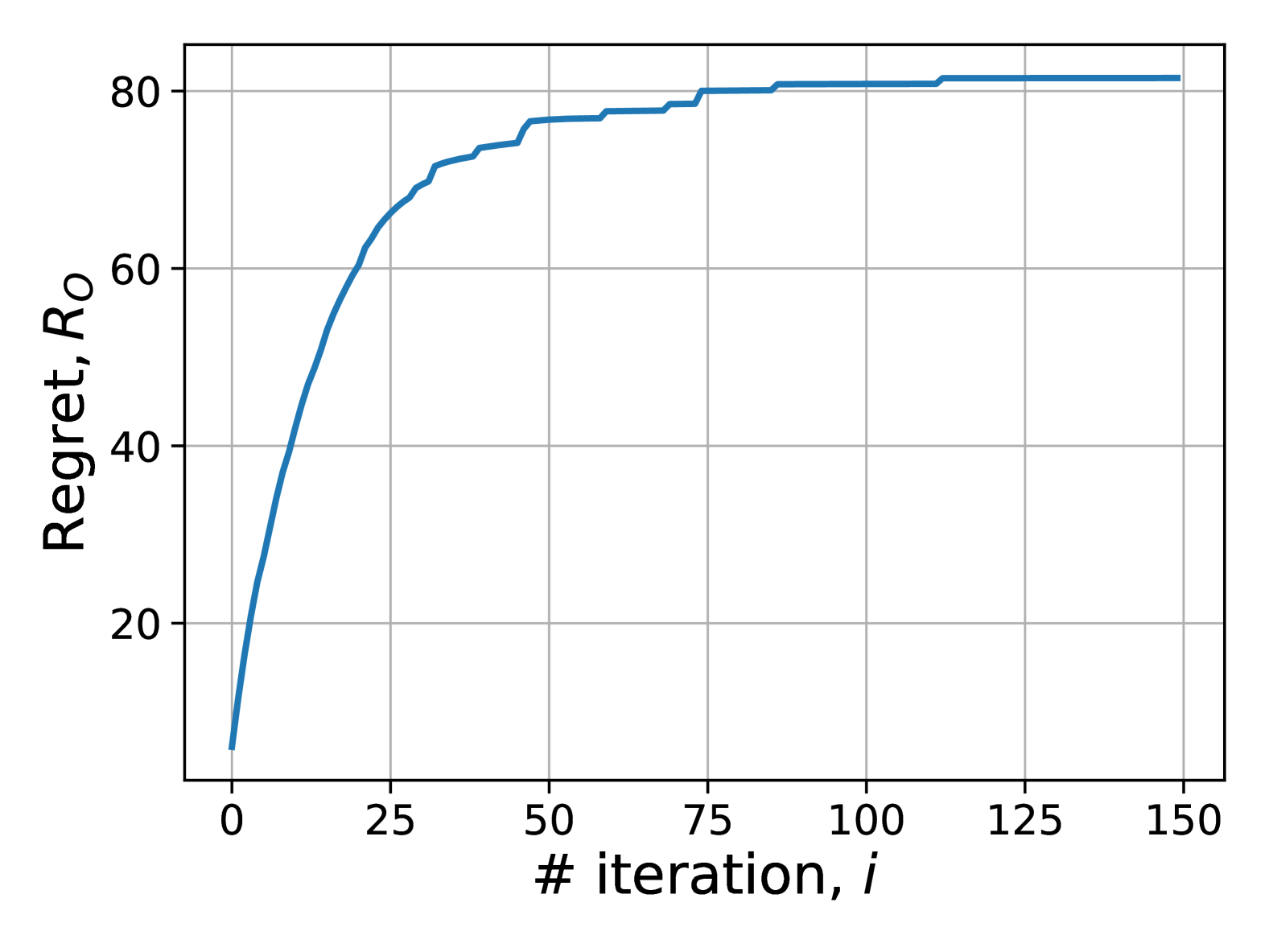
(a) Cumulative regret

(b) Convergence rate

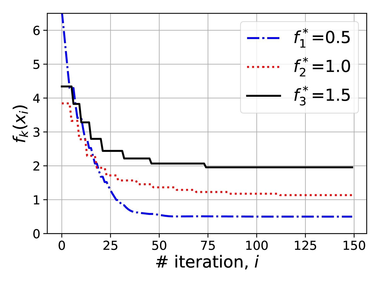
(c) Function values

Figure 1: Dependence of cumulative regret (left), convergence rate (center), and function values (right) on iterations of F-LCB algorithms for FMAB setup with smooth convex functions (21). We see that regret stops growing after some iterations, and our algorithm minimizes only the function with the smallest minimal value.

4.2 FMAB: nonsmooth convex functions

The next testing scenario for our algorithm is the nonsmooth convex setup. We consider piece-wise linear functions:

$$f_{i}(\mathbf{x})=\max_{k=1,\ldots,p}(\mathbf{a}^{\top}_{ki}\mathbf{x}+b_{k}^{i})+c_{i}$$ (22)

and the corresponding feasible sets $D_{i}=[-4,4]^{d_{i}}$. We consider $K=3$ functions and run the algorithm for $T=1000$ steps. We use $p=\{5,10,12\}$ linear functions for given minimal values $[0.5,1,1.5]$ respectively. The dimension of the target variable $\mathbf{x}$ is $d=20$. We use the Subgradient Method with Triple Averaging (SGMTA) [36] as a base optimizer for such functions. For this base optimizer, we have the following $g_{i}(t)=\frac{M_{i}R_{i}}{\sqrt{t}}$. Hence, cumulative regret is bounded by $O\left(RM\sqrt{KT}\right)$. The resulting cumulative regret and function values are presented in Figure 2. The convergence of our F-LCB algorithm demonstrates that the minimization process for the target objective function $f_{1}$ leads to faster convergence to the minimum. In addition, other functions $f_{2}$ and $f_{3}$ are stuck quite far from the minimal values since the better function $f_{1}$ is identified.

(a) Cumulative regret

(b) Convergence rate

(c) Function values

Figure 2: Dependence of cumulative regret (left), convergence rate (center), and functions values (right) on the number of iterations of F-LCB for FMAB setup with nonsmooth convex functions (22). The function with the smallest minimal value among other functions is identified and the smallest minimum is achieved.

4.3 FMAB: smooth convex functions with inexact oracle

To emulate the inexact oracle for the smooth convex setup, we again consider functions (21) but add noise to the gradients. In particular, the gradient estimate is computed as $G_{i}(\mathbf{x},\xi)=\nabla f_{i}(\mathbf{x})+\frac{\sigma_{i}}{\sqrt{d}}\xi$, where $\xi\sim\mathcal{N}(0,I)$. We use stochastic accelerated gradient descent (SAGD) as a base optimizer and parameters from proposition 4.5 in [32] that give $\mathbb{E}[f(\overline{\mathbf{x}}_{t})]-f^{*}\leq O(1)\left(2\gamma R+\frac{4\sqrt{2}(M^{2}+\sigma^{2})}{3\gamma}\right)\frac{1}{\sqrt{t}}$. Therefore, regret is bounded as (18). We consider $K=3$ functions and $T=1500$ steps. The dimension of the target variable is $d=20$, and the variance in the noise is $\sigma=2$. Since setup is stochastic, we run the optimization process 20 times, plot mean values of considered metrics, and show $[0.05,0.95]$ percent confidence interval by shaded area. Figure 3 shows that despite the noise in the gradient estimate, our algorithm finds the best arm. The main difference with the deterministic setup is that the convergence curves shown in Figure 3(b) are less distinguished. However, Figure 3(c) demonstrates that our F-LCB algorithm pays more attention to the minimization of $f_{1}$ rather than $f_{2}$ and $f_{3}$.

(a) Cumulative regret

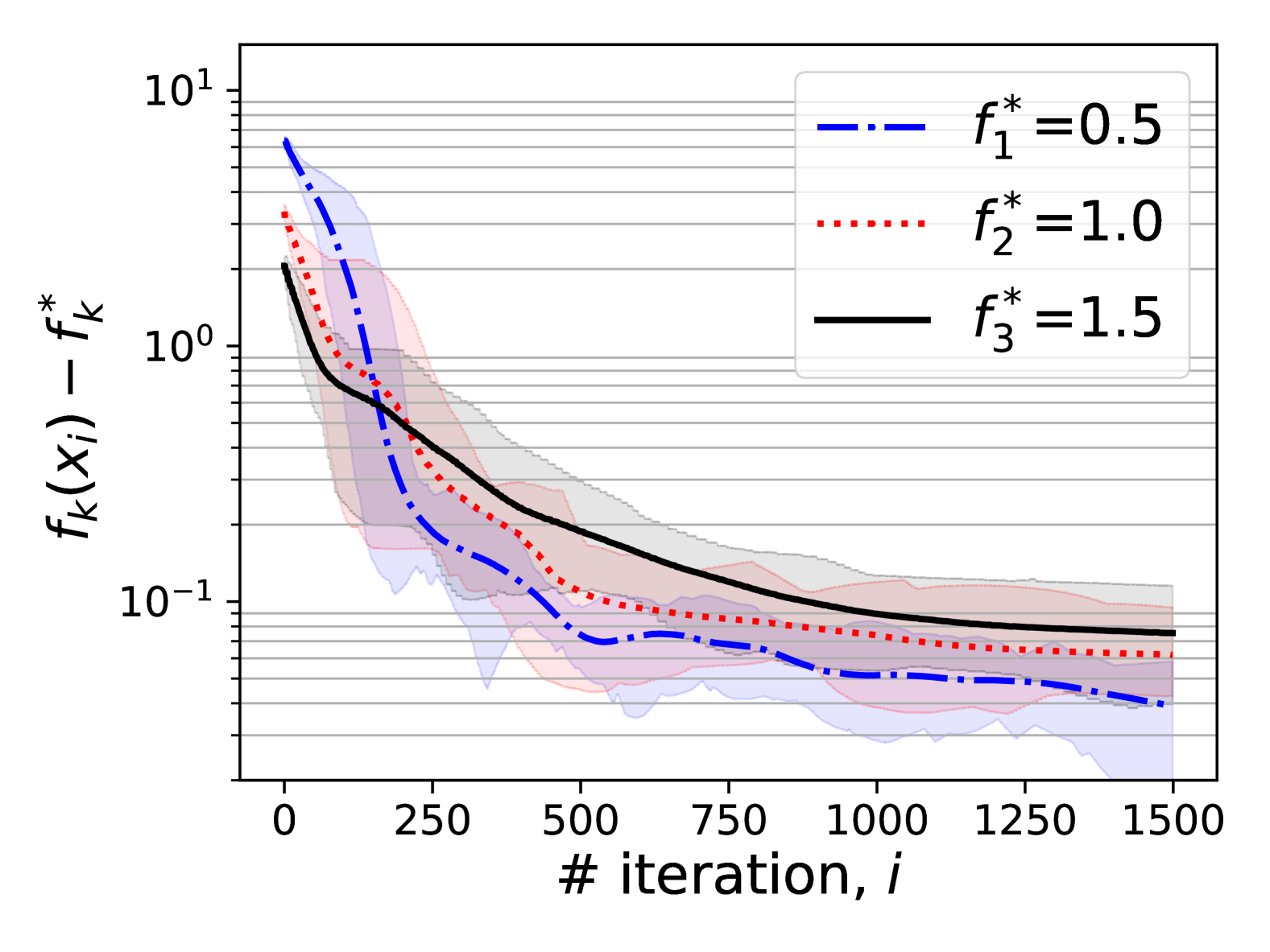
(b) Convergence rate

(c) Function values

Figure 3: Dependence of cumulative regret (left), convergence rate (center), and functions values (right) on iterations of the F-LCB algorithm in the FMAB setup for smooth convex functions with inexact oracles. The function with the smallest minimum is found automatically even in the case of a poor initial guess.

4.4 BFI: neural networks for solving image classification problem

This section considers an application of the proposed F-LCB algorithm to the training neural network models on the CIFAR10 dataset [37]. The main challenge in applying neural networks to sovle practical problem is the choice of the proper architecture for given memory budget of available GPUs. In our experiment, we consider five different models that have almost the same number parameters ($\approx 11.5$M) but structure them in a completely different manner. In particular, we select the following models: ResNet18 [38], convolution neural network similar to VGG [39], which we refer as VGG, shallow MLP with only two large linear layers, which we denote as ShallowMLP and deep MLP with eight linear layers of moderate size, which we denote as DeepMLP. The number of trainable parameters in the considered models is presented in Table 2. Note that DeepMLPNorm has the same structure as DeepMLP except the intermediate normalization layers added to improve stability of the gradient propagation. More detailed description of the considered model can be find in the source code. We expect that our F-LCB algorithm identifies the best neural network architecture to solve image classification task.

Table 2: Number of trainable parameters in the considered candidate neural networks.

Model name	# parameters
ShallowMLP	$12.64$M
DeepMLP	$11.55$M
DeepMLPNorm	$11.57$M
VGG	$11.47$M
ResNet18	$11.17$M

Training hyperparameters.

We use a batch size of 64 and the Adam optimizer [40] with a learning rate of $10^{-4}$. Each arm pull consists of $40$ optimization steps. The budget for F-LCB is $T=200$. We split the entire dataset into three parts: train (45000 samples), validation (5000 samples), and test (10000 samples) sets.

LCB estimation.

In this setup, we define the pull of the $i$-th arm as 40 optimization steps to update the parameters of the $i$-th model based on the minibatches of samples from the training set. After that, validation set is used to evaluate the loss and accuracy of the updated model and update the corresponding LCB. Due to the non-convex nature of the neural network optimization, convergence guarantees do not directly apply. Therefore, we use a heuristic approach motivating by the results from stochastic optimization theory [32] to define the function $g$. In particular, we define $g(t)=\frac{4\cdot f_{i}(x^{1,i})}{\sqrt{t}}$, where a nominator corresponds to the estimate the maximum function devotion during the training process, and $x^{1,i}$ is the parameter vector obtained after the first 40 updates of the initializations. Since neural network training could lead to a large variance in validation losses, we compute the LCB based on the best validation loss for each model obtained up to the current step.

Best model identification results.

We run the proposed algorithm 10 times and report the averaged test loss and test accuracy of the models in Figure 4. In addition, we show the $[0.1,0.9]$ quantile confidence interval via the shaded area. Figure 4 demonstrates that the F-LCB algorithm confidently identifies the two best models. Moreover, the identified models are ResNet18, and VGG which are convolutional neural networks and therefore more efficient in solving the considered image classification problem [41]. In addition, note that ResNet18 dominates VGG during the first 150 iterations of our algorithm. Thus, we confirm that the proposed framework is relevant for the online identification of the best neural network for a particular dataset.

We compare our approach with the naïve baseline based on the early stopping technique. The early stopping technique stops training if the model’s test accuracy does not improve by more than $1\%$ over the consequent $5$ epochs. We subsequently train the considered neural networks with the early stopping technique and identify the best model based on the best test accuracy. This baseline identifies the ResNet18 as the best model, too. However, it requires $19\pm 0.8$ minutes averaged for five runs. At the same time, the proposed F-LCB algorithm identifies the best model only for $9\pm 0.5$ minutes averaged over the same number of runs for 200 pulls, which is enough in our case to estimate best arms. In addition, beyond accelerating model selection, our approach monitors the model training online and provides real-time insights into confidence intervals for models’ learning curves.

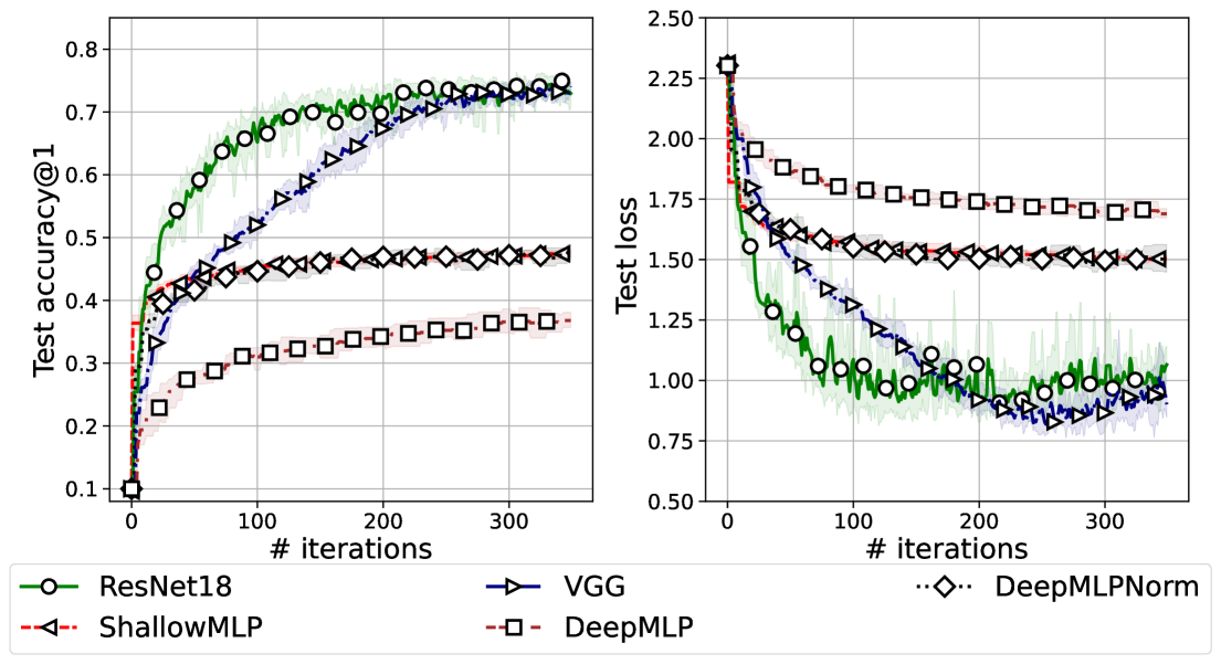
Figure 4: Test accuracy and loss of the considered models. The shaded area shows $[0.1;0.9]$ quantiles after running for 10 times. ResNet18 and VGG models are the most efficient for solving the considered task that coincides with the previous studies.

5 Conclusion

This work investigated strategies for the functional version of the multi-armed bandit problem (FMAB) and a strategy for the best function identification (BFI). It has proposed a simple UCB-type algorithm, F-LCB, that uses basic optimization methods with known large deviation bounds as a routine to construct LCB estimates on arms. It also establishes regret rate guarantees for FMAB and deterministic BFI problems.

Extensions of this work may concentrate on the following problems. (i) What is the lower bound for stochastic FMAB? (ii) Suppose that our subproblems are not purely black-box and we have access to the dual subproblem. It could be used to construct new LCB estimates. Could we do better with this duality-based LCB? (iii) Usually, we cannot guarantee convergence rates even when oracles are exact for the non-convex case. Could we use other estimation techniques to supplement, for example, the Adam algorithm as a base for FMAB and make it usable to train LLM-type models?

Appendix A Lower bounds

Next we show that lower bounds for BFI problem setting could be derived from lower bounds for related optimization problems. We establish them for deterministic algorithms. Next we proceed with a general reduction scheme to obtain lower bounds for our problem based on lower bounds for respective optimization problems.

Denote by $\mathcal{P}_{i}$ ($1\leq i\leq k$) optimization problem

$$\min_{x\in\mathcal{D}_{i}}f_{i}(x),$$

and by $f_{i}^{*}$ the value of the objective at the solution. For simplicity reasons, we assume that objective functions are from the same class $f_{1},\dots,f_{k}\in\mathcal{F}$ and that each function is equipped with the oracle from the same class and feasibility sets $\mathcal{D}_{i}$ are nonempty convex sets with the same difficulty for oracles. The complexity of each $\mathcal{P}_{i}$ (in terms of [29]) is the same, i.e. each problem has the same lower bound. To make it more precise, there exists a function $g(H,t)$ such that for each algorithm $\mathcal{A}$ and resulting sequence of feasible test points $\{x_{t}\}_{t=1}^{\infty}$ defined as $x_{t+1}=\mathcal{A}\left(x_{1},\mathcal{O}(x_{1}),\dots,x_{t},\mathcal{O}(x_{t})\right)$ there exists a problem instance $\mathcal{P}$ defined by parameters $H=(f,\mathcal{D})$ and oracle $\mathcal{O}$ the following inequation holds:

$$f(x_{t})-\min_{x\in\mathcal{D}}f(x)\geq g(H,t).$$ (23)

Function $g(H,t)$ is much easier to comprehend if it can be factorized as $g(H,t)=\phi(H)\cdot t^{-\alpha}$ and then used $\Omega(t^{-\alpha})$ notation instead. For example, in the case of unconstrained minimizing a smooth convex objective equipped with a first-order oracle, in the seminal work [29] shows that optimal rates are $t^{-2}$. We will call lower bound sharp and uniform for an algorithm family $\mathcal{W}=\{\mathcal{A}\}$ and problem family $\mathcal{S}=\{\mathcal{P}\}$ such that for any algorithm $\mathcal{A}$ from $\mathcal{W}$ there exists a problem $\mathcal{P}$ such that the following equality holds $f(x_{t})-\min_{x\in\mathcal{D}}f(x)\geq g(H_{\mathcal{P}},t)$ for each time $t>0$.

We also need to introduce the concept of optimal algorithm, i.e. the algorithm $\mathcal{A}^{*}$ with convergence rate same as lower bound up to constant:

$$f(x_{t})-\min_{x\in\mathcal{D}}f(x)\leq C_{\mathcal{A}^{*}}g(H,t),$$ (24)

where $C_{\mathcal{A}^{*}}>0$ is some known constant.

For the problem of unconstrained minimization of smooth convex objectives equipped with a first-order oracle, the renowned Nesterov’s accelerated gradient descent (AGD) [34] is optimal. Actually, monotone version of AGD is needed, since we introduce uniform lower bound, that holds for each time step $t$.

A.1 Best function identification problem

Assuming that the agent has access to the optimal algorithm $\mathcal{A}$ for the problem class of problems $\mathcal{P}_{1},\dots,\mathcal{P}_{k}$ with exact lower bound defined by the function $g(H,t)$, what is the lower bound for the optimal arm identification problem?

More formally, what number of testing points is needed to certify that $R(T)\leq\varepsilon$?

Let $\mathcal{P}_{1}$ and $\mathcal{P}_{2}$ be two problem instances from the same class with optimal values $f_{1}^{*}$ and $f_{2}^{*}$ respectively.

Denote by $t_{i}(\varepsilon)=t(\varepsilon,H_{i})=\{\min t\mid g(H_{i},t)\leq\varepsilon\}$ the vicinity hitting time for the problem defined by $\mathcal{H}_{i}$ and tolerance level $\varepsilon$. In case of sharp lower bounds we assume that for each algorithm $\mathcal{A}$ there exists hard problem $\mathcal{P}$ such that if $t>t_{i}(\varepsilon)$, then $f(x_{t})-f^{*}<\varepsilon$.

Let $\mathcal{A}$ be an algorithm supported by the oracle $\mathcal{O}(x)$ and the sequence of points it generates $\{x_{t}\}_{t=1}^{\infty}$ such that $x_{t+1}=\mathcal{A}\left(x_{1},\mathcal{O}(x_{1}),\dots,x_{t},\mathcal{O}(x_{t})\right)$ for all $t$.

Denote by $\mathcal{L}(\mathcal{G})=\{\mathcal{L}_{t}(\mathcal{G})\}_{t=1}^{\infty}$ the sequence of problem sets, such that $\mathcal{L}_{t}(\mathcal{G})=\{\mathcal{P}\quad|\quad x_{s}^{\mathcal{P}}=x_{s}^{\mathcal{G}},\quad\mathcal{O}_{\mathcal{G}}(x_{s}^{\mathcal{G}})=\mathcal{O}_{\mathcal{P}}(x_{s}^{\mathcal{P}}),\quad 1\leq s\}$, i.e. $\mathcal{L}_{t}$ is a set of problems that could not be distinguished by any algorithm $\mathcal{A}$ with supporting oracle $\mathcal{O}$ until step $t$.

Let $\mathcal{P}_{1}$ and $\mathcal{P}_{2}$ be two problem instances from the same class.

Lemma 1.

Consider the best function identification problem consisting of two problems from a given class with uniform sharp lower bound function $g(H,t)$. Then achieving regret $R_{B}(T)\leq\varepsilon$ requires at least

$$T\geq 2\cdot t(\varepsilon)$$

testing points.

Proof.

Note that to certify that $R_{B}(T)\leq\varepsilon$ one needs either to show that $|f_{1}^{*}-f_{2}^{*}|\leq\varepsilon$ or to identify the index of the optimal function $i^{*}=\arg\min_{i={1,2}}f_{i}^{*}$.

Suppose that the algorithm tries to solve the best arm identification problem for $\mathcal{P}_{1}$ and $\mathcal{P}_{2}$, runs $\hat{t}_{1}$ and $\hat{t}_{2}$ iterations for problem $\mathcal{P}_{1}$ and $\mathcal{P}_{2}$ respectively and then makes a decision. Then it must make the same decision for any problem pair $(\hat{\mathcal{P}}_{1},\hat{\mathcal{P}}_{2})$ such that $\hat{\mathcal{P}}_{1}\in L_{\hat{t}_{1}}(\mathcal{P}_{1})$ and $\hat{\mathcal{P}}_{2}\in L_{\hat{t}_{2}}(\mathcal{P}_{2})$.

Let $\mathcal{P}$ be hard problem for a given algorithm $\mathcal{A}$, i.e. such that inequality 23 holds. Let $f^{*}$ be the optimal value in $\mathcal{P}$ and $t(\varepsilon)$ denote vicinity hitting time for $(\mathcal{A},\mathcal{P})$.

Suppose that $\mathcal{P}_{1}\in\mathcal{L}_{\hat{t}_{1}-1}(\mathcal{P})$ and $\mathcal{P}_{2}\in\mathcal{L}_{\hat{t}_{2}-1}(\mathcal{P})$, i.e. problems could not be distingueshed by the algorithm.

Next let us fix computational budgets and show that there exist setup such that it would be not sufficient to guarantee $R(T)\leq\varepsilon$.

Let us fix any positive numbers $\hat{t}_{1}$ and $\hat{t}_{2}$ such that $\hat{t}_{1}+\hat{t}_{2}=T$ and assume that $2\cdot t(\varepsilon)>T$. Then at least one inequality holds: $\hat{t}_{1}<t(\varepsilon)$, or $\hat{t}_{2}<t(\varepsilon)$, or both $\hat{t}_{1}<t(\varepsilon)$ and $\hat{t}_{2}<t(\varepsilon)$.

W.l.o.g. assume that $\hat{t}_{1}<t(\varepsilon)$.

Suppose that the algorithm picks $f_{1}$ as a solution. Then we can pick feasible problem pair $\mathcal{P}_{1}\in\mathcal{L}_{\hat{t}_{1}-1}(\mathcal{P})$, $f_{1}^{*}=f_{2}(x_{\hat{t}_{1}^{\mathcal{P}}})$ and $\mathcal{P}_{2}=\mathcal{P}$. For this problem pair it is known that optimal arm is $\mathcal{P}_{2}$, and regret could be estimated as follows.

$$R_{B}(T)=f_{1}^{*}-f_{2}^{*}=f_{2}(x_{\hat{t}_{1}^{\mathcal{P}}})-f^{*}_{2}\geq g(\mathcal{P},\hat{t}_{1})>\varepsilon$$

Suppose that algorithm picks $f_{2}$ as a solution. Then we could pick feasible problem pair $\mathcal{P}_{1}\in\mathcal{L}_{\hat{t}_{1}-1}(\mathcal{P})$, $f_{1}^{*}<f^{*}-\varepsilon$ and $\mathcal{P}_{2}=\mathcal{P}$. In this case problem $\mathcal{P}_{1}$ mask itself as $\mathcal{P}$ until round $\hat{t}_{1}$ and is not restricted after. ∎

This leads to a trivial corollary that the best function identification problem with $k$ arms requires at least $T\geq k\cdot t(\varepsilon)$ iterations to guarantee $R_{B}(T)\leq\varepsilon$.

References

- [1] Martin Zinkevich. Online convex programming and generalized infinitesimal gradient ascent. In Proceedings of the 20th international conference on machine learning (icml-03), pages 928–936, 2003.
- [2] Shai Shalev-Shwartz et al. Online learning and online convex optimization. Foundations and Trends® in Machine Learning, 4(2):107–194, 2012.
- [3] Elad Hazan et al. Introduction to online convex optimization. Foundations and Trends® in Optimization, 2(3-4):157–325, 2016.
- [4] Francesco Orabona. A modern introduction to online learning. arXiv preprint arXiv:1912.13213, 2019.
- [5] Abraham D Flaxman, Adam Tauman Kalai, and H Brendan McMahan. Online convex optimization in the bandit setting: gradient descent without a gradient. arXiv preprint cs/0408007, 2004.
- [6] William R Thompson. On the likelihood that one unknown probability exceeds another in view of the evidence of two samples. Biometrika, 25(3-4):285–294, 1933.
- [7] Herbert Robbins. Some aspects of the sequential design of experiments. 1952.
- [8] Nicolo Cesa-Bianchi and Gábor Lugosi. Prediction, learning, and games. Cambridge university press, 2006.
- [9] Sébastien Bubeck, Nicolo Cesa-Bianchi, et al. Regret analysis of stochastic and nonstochastic multi-armed bandit problems. Foundations and Trends® in Machine Learning, 5(1):1–122, 2012.
- [10] Aleksandrs Slivkins et al. Introduction to multi-armed bandits. Foundations and Trends® in Machine Learning, 12(1-2):1–286, 2019.
- [11] Tor Lattimore and Csaba Szepesvári. Bandit algorithms. Cambridge University Press, 2020.
- [12] Peter Auer, Nicolo Cesa-Bianchi, Yoav Freund, and Robert E Schapire. The nonstochastic multiarmed bandit problem. SIAM journal on computing, 32(1):48–77, 2002.
- [13] Sébastien Bubeck and Aleksandrs Slivkins. The best of both worlds: Stochastic and adversarial bandits. In Conference on Learning Theory, pages 42–1. JMLR Workshop and Conference Proceedings, 2012.
- [14] Julian Zimmert and Yevgeny Seldin. Tsallis-inf: An optimal algorithm for stochastic and adversarial bandits. Journal of Machine Learning Research, 22(28):1–49, 2021.
- [15] Sébastien Bubeck, Gilles Stoltz, Csaba Szepesvári, and Rémi Munos. Online optimization in x-armed bandits. Advances in Neural Information Processing Systems, 21, 2008.
- [16] Sébastien Bubeck, Rémi Munos, Gilles Stoltz, and Csaba Szepesvári. X-armed bandits. Journal of Machine Learning Research, 12(5), 2011.
- [17] Long Tran-Thanh and Jia Yuan Yu. Functional bandits. arXiv preprint arXiv:1405.2432, 2014.
- [18] Michael Woodroofe. A one-armed bandit problem with a concomitant variable. Journal of the American Statistical Association, 74(368):799–806, 1979.
- [19] Naoki Abe, Alan W Biermann, and Philip M Long. Reinforcement learning with immediate rewards and linear hypotheses. Algorithmica, 37:263–293, 2003.
- [20] Aleksandrs Slivkins. Contextual bandits with similarity information. In Proceedings of the 24th annual Conference On Learning Theory, pages 679–702. JMLR Workshop and Conference Proceedings, 2011.
- [21] Wei Chu, Lihong Li, Lev Reyzin, and Robert Schapire. Contextual bandits with linear payoff functions. In Proceedings of the Fourteenth International Conference on Artificial Intelligence and Statistics, pages 208–214. JMLR Workshop and Conference Proceedings, 2011.
- [22] Rajeev Agrawal. The continuum-armed bandit problem. SIAM journal on control and optimization, 33(6):1926–1951, 1995.
- [23] Robert Kleinberg, Aleksandrs Slivkins, and Eli Upfal. Multi-armed bandits in metric spaces. In Proceedings of the fortieth annual ACM symposium on Theory of computing, pages 681–690, 2008.
- [24] Sarah Filippi, Olivier Cappe, Aurélien Garivier, and Csaba Szepesvári. Parametric bandits: The generalized linear case. Advances in neural information processing systems, 23, 2010.
- [25] Xinyi Zhang, Zhuo Chang, Hong Wu, Yang Li, Jia Chen, Jian Tan, Feifei Li, and Bin Cui. A unified and efficient coordinating framework for autonomous dbms tuning. Proceedings of the ACM on Management of Data, 1(2):1–26, 2023.
- [26] Wentao Wu and Chi Wang. Budget-aware query tuning: An automl perspective. ACM SIGMOD Record, 53(3):20–26, 2024.
- [27] Jean-Yves Audibert and Sébastien Bubeck. Best arm identification in multi-armed bandits. In COLT-23th Conference on learning theory-2010, pages 13–p, 2010.
- [28] Julia Gusak, Daria Cherniuk, Alena Shilova, Alexandr Katrutsa, Daniel Bershatsky, Xunyi Zhao, Lionel Eyraud-Dubois, Oleh Shliazhko, Denis Dimitrov, Ivan V Oseledets, et al. Survey on efficient training of large neural networks. In IJCAI, pages 5494–5501, 2022.
- [29] Arkadi Nemirovsky and David Yudin. Problem complexity and method efficiency in optimization. 1983.
- [30] Peter Auer. Using confidence bounds for exploitation-exploration trade-offs. Journal of Machine Learning Research, 3(Nov):397–422, 2002.
- [31] Yuriy Dorn, Aleksandr Katrutsa, Ilgam Latypov, and Andrey Pudovikov. Fast ucb-type algorithms for stochastic bandits with heavy and super heavy symmetric noise. arXiv preprint arXiv:2402.07062, 2024.
- [32] Guanghui Lan. First-order and stochastic optimization methods for machine learning, volume 1. Springer, 2020.
- [33] Weijie Su, Stephen Boyd, and Emmanuel J Candes. A differential equation for modeling nesterov’s accelerated gradient method: Theory and insights. Journal of Machine Learning Research, 17(153):1–43, 2016.
- [34] Y Nesterov. A method for solving a convex programming problem with convergence rate . In Soviet Mathematics. Doklady, volume 27, pages 367–372, 1983.
- [35] Adrien B Taylor, Julien M Hendrickx, and François Glineur. Exact worst-case performance of first-order methods for composite convex optimization. SIAM Journal on Optimization, 27(3):1283–1313, 2017.
- [36] Yu Nesterov and Vladimir Shikhman. Quasi-monotone subgradient methods for nonsmooth convex minimization. Journal of Optimization Theory and Applications, 165(3):917–940, 2015.
- [37] Alex Krizhevsky and Geoffrey Hinton. Learning multiple layers of features from tiny images. Technical report, University of Toronto, 2009.
- [38] Kaiming He, Xiangyu Zhang, Shaoqing Ren, and Jian Sun. Deep residual learning for image recognition. In Proceedings of the IEEE conference on computer vision and pattern recognition, pages 770–778, 2016.
- [39] Karen Simonyan and Andrew Zisserman. Very deep convolutional networks for large-scale image recognition. arXiv preprint arXiv:1409.1556, 2014.
- [40] Diederik P Kingma. Adam: A method for stochastic optimization. arXiv preprint arXiv:1412.6980, 2014.
- [41] Ian Goodfellow, Yoshua Bengio, Aaron Courville, and Yoshua Bengio. Deep learning, volume 1. MIT press Cambridge, 2016.