A nodally bound-preserving finite element method for time-dependent convection-diffusion equations

Abstract

This paper presents a new method to approximate the time-dependent convection-diffusion equations using conforming finite element methods, ensuring that the discrete solution respects the physical bounds imposed by the differential equation. The method is built by defining, at each time step, a convex set of admissible finite element functions (that is, the ones that satisfy the global bounds at their degrees of freedom) and seeks for a discrete solution in this admissible set. A family of $\theta$-schemes is used as time integrators, and well-posedness of the discrete schemes is proven for the whole family, but stability and optimal-order error estimates are proven for the implicit Euler scheme. Nevertheless, our numerical experiments show that the method also provides stable and optimally-convergent solutions when the Crank-Nicolson method is used.

[label1]organization= Department of Mathematics and Statistics, University of Strathclyde, addressline=26 Richmond Street, postcode=G1 1XH, city=Glasgow, country=Scotland

[label2]organization=Department of Mathematical Sciences, addressline=University of Bath , city=Claverton down, Bath, postcode=BA2 7AY, country=UK

1 Introduction

In many applications the simulation of time-dependent convection-diffusion equations is required. The solution of this equation provides a theory for the transport-controlled reaction rate of two molecules in a shear flow, also it models the processes of the chemical reaction in a flow field. Such simulations are obtained by a nonlinear system of time dependent convection-diffusion equations for the concentrations of the reactants and the products. An inaccuracy in one of the equations in the system of nonlinear equations affects all the concentrations. Usually in applications the convection field is dominant over the diffusion by several orders of magnitude, thus making the numerical approximation of such problems very unstable and prone to spurious oscillations. For example, it is well-known that the standard Galerkin finite element method for space discretisation is not appropriate for convection-dominated problems. The preferred way to deal with this fact over the last few decades has been to replace the standard Galerkin finite element method by a stabilised finite element method, that is, a method that adds an extra term to the formulation in such a way that stability is enhanced. The first stabilised methods for convection-diffusion problems, e.g., the SUPG method [1] and the Galerkin Least-Squares method [2] were of residual type, i.e., a weighted term based on the residual was added to the formulation to add numerical diffusion. In the time dependent context the residual character of the SUPG method requires the time derivative of the solution to be included in the stabilisation term, thus creating a somewhat artificial coupling between the time step and the stabilisation parameter. This coupling has been extensively studied in the literature, see, e.g.,[3] where stability is analysed for different choices of time discretisation. In fact, if a standard stability analysis is performed, the addition of SUPG stabilisation suggests a loss of stability if the mesh size and time step are not correctly balanced (although some numerical evidence contradicting this claim can be found, e.g., in [4]). Due to this, in later years the possibilty of using non-residual, symmetric stabilisations for the time-dependent convection-diffusion has been studied more intensively. Examples of symmetric stabilisations include the subgrid viscosity method [5], the orthogonal subscale method [6], and the continuous interior penalty (CIP) method [7]. In the work [8] a detailed analysis on the stability analysis and advantages of using symmetric stabilisation can be found.

Now, none of the methods mentioned in the previous paragraph can be proven to satisfy the so-called Discrete Maximum Principle (DMP), or even the weaker property of respecting the bounds satisfied by the continuous problem. In fact, this property has been derived for only a selection of methods, usually under geometric conditions on the computational mesh. For example, in the pioneering work [9] it is shown that for the finite element discretisation of a diffusion equation in two space dimensions using piecewise linear elements a sufficient condition for the satisfaction of the DMP is that the mesh satisfies the Delaunay condition. This condition was then proven necessary for the matrix to have the right sign pattern in the later work [10]. The situation is more dramatic for convection-diffusion equations, where the mesh needs to be acute, and sufficiently fine, for the matrix to have the right sign pattern, and thus the finite element method to satisfy the DMP. For convection-diffusion equations, the more straightforward remedy is to add isotropic artificial diffusion to the problem, in such a way that the dominating matrix in the linear system is the diffusion one. This strategy does lead to a method that satisfies the DMP under less stringent conditions on the fineness of the mesh. Unfortunately, the consistency error introduced by adding artificial diffusion is too large, and the results obtained by this method tend to smear the layers excessively (see, e.g., [11, Section 5.2] for a discussion and further references). In the quest of adding diffusion so the DMP is satisfied and layers are not excessively smeared, the idea of localising the diffusion has been proposed as a way to make the problem locally diffusion-dominated in areas near extrema and layers, thus preventing spurious oscillations and local violations of the discrete maximum principle. This leads to nonlinear (shock-capturing related) discretisations. In the last few decades numerous nonlinear discretisations for the steady-state convection-diffusion equation have been proposed, e.g., [12, 10, 13, 14, 15], and [11] for a review.

In many instances, the numerical solution does not need to be completely free of local spurious oscillations; it only needs to satisfy global bounds to lead to a stable discretisation. One way to achieve a solution that respects this bound is to simply cut the solution at the bound, like it is done in, e.g., the cut-off finite element method [16]. However, this process results in a solution that is not an element of the finite element space, and thus analysing its stability and convergence is, in general, a challenging affair. In the recent works [17, 18] an alternative path is followed. It uses the following property: There is a correspondence between the imposition of bounds on the numerical solution and searching for the numerical solution on a convex subset of the finite element space of the steady state convection-diffusion equation consisting of the discrete functions satisfying those bounds at their nodal values. So, in those works a finite element method that seeks directly for a finite element solution that satisfies the global bounds is proposed, and analysed in different contexts. In this work we build on those previous works and extend that method to the time dependent convection-diffusion equation. The basic idea can be summarised as follows: for each time step we define a set $V_{\mathcal{P}}^{+}$, of admissible finite element functions as those satisfying the global bound at at their degrees of freedom (nodal values in the case of Lagrangian elements); then, introduce an algebraic projection onto the admissible set, denote by $u_{h}^{+}$ the projection of $u_{h}$ onto $V_{\mathcal{P}}^{+}$ and write a finite element problem for the projected object. To eliminate the non-trivial kernel (and so to remove the singularity) generated by this process, a stabilisation term is incorporated into the discretised equations at each time step to remove this kernel (that is, the part of the solution which has been removed). In our numerical experience we have observed that more stable results are obtained if we add a linear stabilised term to the problem for $u_{h}^{+}$, and thus we present the method including CIP stabilisation.

The remainder of the paper is organised as follows: In Section 2 we introduce the notation, the model problem, and all the preliminary material for the setup of the method. In Section 3 we present the finite element method and show its well-posedness. The stability and error analysis is carried out in Section 4, and in Section 5 we test the performance of the method via different numerical experiments. Finally, some conclusions are drawn in Section 6.

2 General setting and the model problem

We will adopt standard notations for Sobolev spaces in line with, e.g., [19]. For $D\subseteq\mathbb{R}^{d}$, $d=1,2,3$, we denote by $\|\cdot\|_{0,p,D}$ the $L^{p}(D)$-norm; when $p=2$ the subscript $p$ will be omitted and we only write $\|\cdot\|_{0,D}$. The inner product in $L^{p}(D)$ is also denoted by $(\cdot,\cdot)_{D}$. In addition, for $s\geq 0$, $p\in[1,\infty]$, we denote by $\|\cdot\|_{s,p,D}$ ($|\cdot|_{s,p,D}$) the norm (seminorm) in $W^{s,p}(D)$; when $p=2$, we define $H^{s}(D)=W^{s,2}(D)$, and again omit the subscript $p$ and only write $\|\cdot\|_{s,D}$ ($|\cdot|_{s,D}$). The following space will also be used repeatedly within the text

$$H^{1}_{0}(D)=\left\{v\in H^{1}(D):v=0\;{\rm on}\;\partial D\right\}.$$ (1)

For $1\leq p\leq+\infty$, $L^{p}((0,T);W^{s,p}(D))$ is the space defined by

$$L^{p}((0,T);W^{s,p}(D))=\left\{u(t,\cdot)\in W^{s,p}(D)~~\text{for almost all $t\in[0,T]$}:\|u\|_{s,p,D}\in L^{p}(0,T)\right\}\,,$$

and it is a Banach space for the norm

$$\begin{split}\|u\|_{L^{p}((0,T);W^{s,p}(D))}=\left\{\begin{array}[]{ll}\left(\int_{0}^{T}\|u\|_{s,p,D}^{p}\textrm{d}t\right)^{\frac{1}{p}}\hskip 65.44142pt{\rm if}\hskip 5.69046pt1\leq p<\infty,\\ \\ {\rm ess}\hskip 1.42271pt\sup_{t\in(0,T)}\|u\|_{s,p,D}\hskip 54.06006pt{\rm if}\hskip 8.5359ptp=\infty.\end{array}\right.\end{split}$$

2.1 The model problem

Let $\Omega$ be an open bounded Lipschitz domain in $\mathbb{R}^{d}$ ($d=2,3$) with polyhedral boundary $\partial\Omega$, and $T>0$. For a given $f\in L^{2}((0,T);L^{2}(\Omega))$, we consider the following convection-diffusion problem:

$$\begin{split}\left\{\begin{aligned} \partial_{t}u-\varepsilon\,\Delta u+{\boldsymbol{\beta}}\cdot\nabla u+\mu u&=f&&\text{in }(0,T]\times\Omega,\\ u(\boldsymbol{x},t)&=0&&\text{on }(0,T]\times\partial\Omega,\\ u(\cdot,0)&=u^{0}&&\text{in }\Omega,\end{aligned}\right.\end{split}$$ (2)

where $\varepsilon\in\mathbb{R}^{+}$, ${\boldsymbol{\beta}}=(\beta_{i})_{i=1}^{d}\in L^{\infty}((0,T);W^{1,\infty}(\Omega))^{d}$, and $\mu\in\mathbb{R}^{+}_{0}$, respectively, are the diffusion coefficient, the convective field, and the reaction coefficient. We will assume that ${\rm div}{\boldsymbol{\beta}}=0$ in $\Omega\times[0,T]$.

The standard weak formulation of (2) reads as follows: Find $u\in L^{\infty}((0,T),H^{1}_{0}(\Omega))\cap H^{1}((0,T),H^{-1}(\Omega))$ such that, for almost all $t\in(0,T)$ the following holds

$$\begin{split}\left\{\begin{array}[]{ll}(\partial_{t}u,v)_{\Omega}+a(u,v)=(f,v)_{\Omega}\hskip 28.45274pt\forall v\in H^{1}_{0}(\Omega),\\ \hskip 45.52458ptu(\cdot,0)=u^{0}.\end{array}\right.\end{split}$$ (3)

Here, the bilinear form $a(\cdot,\cdot)$ is defined by

$$a(w,v):=\varepsilon\left(\nabla w,\nabla v\right)_{\Omega}+({\boldsymbol{\beta}}\cdot\nabla w,v)_{\Omega}+\mu(w,v)_{\Omega}\hskip 28.45274pt\forall v\in H^{1}_{0}(\Omega),\hskip 11.38092ptt\in(0,T).$$ (4)

In the above definition we have slightly abused the notation, as the convective term ${\boldsymbol{\beta}}$ might depend on $t$, but unless the context requires it, we will always denote this bilinear form by $a(\cdot,\cdot)$. Since we have supposed that ${\boldsymbol{\beta}}$ is solenoidal, for each $t\in(0,T)$ the bilinear form $a(\cdot,\cdot)$ induces the following “energy” norm in $H^{1}_{0}(\Omega)$

$$\|v\|_{a}=\sqrt{a(v,v)}\hskip 11.38092ptt\in[0,T].$$

The well-posedness of (3) is a well-studied problem. In fact, this is a consequence of Lions’ Theorem (see, e.g., [20, Theorem 10.9]). Moreover, as a consequence of the maximum principle for parabolic partial differential equations (see, e.g., [21, Theorem 12, Section 7.1]), the solution of (3) reaches its extrema on $\big{[}\Omega\times\{0\}\big{]}\cup\big{[}\partial\Omega\times(0,T]\big{]}$ if $f=0$, and its extrema depend also on the values of $f$ otherwise. Motivated by this, we make the following assumption on $u$, solution of (3).

Assumption (A1): We will suppose that the weak solution of (3) satisfies

$$0\leq u(\boldsymbol{x},t)\leq\kappa(t)\hskip 14.22636pt\text{for almost all}\ \ (\boldsymbol{x},t)\in\Omega\times[0,T],$$ (5)

where $\kappa(t)$ is a known positive function dependent on $t$.

In the above assumption, the lower bound in (5) is not required to be zero; however, we set it to zero for the sake of clarity in the explanation. Additionally, the results presented in this work will remain valid if $\kappa(t)$ is replaced by a positive function $\kappa(\boldsymbol{x},t)$.

2.2 Space discretisation

As it is usual in the discretisation of parabolic partial differential equations, we first discretise (3) only in space. To build a finite element space of $H^{1}_{0}(\Omega)$, let ${\mathcal{P}}$ be a conforming, shape-regular partition of $\Omega$ into simplices (or affine quadrilaterals/hexahedra). Over ${\mathcal{P}}$, and for $k\geq 1$, we define the finite element space

$$V_{\mathcal{P}}:=\{v_{h}\in C^{0}(\overline{\Omega}):v_{h}|_{K}\in\mathfrak{R}(K)\ \ \ \forall K\in{\mathcal{P}}\}\cap H^{1}_{0}(\Omega),$$ (6)

where

$$\mathfrak{R}(K)=\left\{\begin{array}[]{ll}\mathbb{P}_{k}(K),\hskip 28.45274pt\text{ if $K$ is a simplex},\\ \mathbb{Q}_{k}(K),\hskip 28.45274pt\text{ if $K$ is an affine quadrilateral/hexahedron},\end{array}\right.$$ (9)

where $\mathbb{P}_{k}(K)$ denotes the polynomials of total degree $k$ on $K$ and $\mathbb{Q}_{k}(K)$ denotes the mapped space of polynomial of degree of at most $k$ in each variable.

For a mesh $\mathcal{P}$, the following notations are used:

• let $\{\boldsymbol{x}_{1},\boldsymbol{x}_{2},\ldots,\boldsymbol{x}_{N}\}$ denote the set of internal nodes; the usual Lagrangian basis functions associated to these nodes, spanning the space $V_{{\mathcal{P}}}$, are denoted by $\phi_{1},\ldots,\phi_{N}$;

• let $\mathcal{F}_{I}$ denote the set of internal facets, $\mathcal{F}_{\partial}$ denote the set of boundary facets of ${\mathcal{P}}$; $\mathcal{F}_{h}=\mathcal{F}_{I}\cup\mathcal{F}_{\partial}$ denote the set of all facets of ${\mathcal{P}}$; for an element $K\in{\mathcal{P}}$ the set of its facets is denoted by $\mathcal{F}_{K}$;

• for a facet $F\in\mathcal{F}_{I}$, $\llbracket\cdot\rrbracket$ denotes the jump of a function across $F$.

The diameter of a set $G\subset\mathbb{R}^{d}$ is denoted by $h_{G}$, and the mesh size is defined as $h=\max\{h_{K}:K\in\mathcal{P}\}$. We also define the mesh function $\mathfrak{h}$ as a continuous, element-wise linear function that represents a local average of element diameters, commonly used in finite element analysis [22]. To construct this, we introduce the set of vertices of the mesh, $\boldsymbol{v}_{1},\ldots,\boldsymbol{v}_{M}$, and define $\mathfrak{h}$ as the piecewise linear function specified by the nodal values

$$\mathfrak{h}(\boldsymbol{v}_{i})=\dfrac{\sum_{K:\boldsymbol{v}_{i}\in K}h_{K}}{\#\{K:\boldsymbol{v}_{i}\in K\}}\,.$$ (10)

In the construction of the method, and its analysis, the following mass-lumped $L^{2}$-inner product will be of importance: for every $v_{h},w_{h}\in V_{\mathcal{P}}$, we define

$$(v_{h},w_{h})_{h}=\sum_{i=1}^{M}\mathfrak{h}(\boldsymbol{x}_{i})^{d}v_{h}(\boldsymbol{x}_{i})w_{h}(\boldsymbol{x}_{i}),$$ (11)

which induces the norm $\lvert v_{h}\lvert_{h}:=(v_{h},v_{h})_{h}^{\frac{1}{2}}$ in $V_{\mathcal{P}}$. This norm is, in fact, equivalent to the standard $L^{2}(\Omega)$-norm. More precisely, the following result, whose proof can be found in [23, Propositions 28.5, 28.6], will be used repeatedly in our analysis below: There exist $C,c>0$, independent of $h$, such that

$$c\,\sum_{i:\boldsymbol{x}_{i}\in K}h_{K}^{d}v_{h}^{2}(\boldsymbol{x}_{i})\leq\|v_{h}\|_{0,K}^{2}\leq C\,\sum_{i:\boldsymbol{x}_{i}\in K}h_{K}^{d}v_{h}^{2}(\boldsymbol{x}_{i})\qquad\forall\,K\in{\mathcal{P}},~~\forall v_{h}\in V_{{\mathcal{P}}},$$ (12)

and thus, as a consequence of the shape-regularity of the mesh, the following holds:

$$c\,|v_{h}|_{h}^{2}\leq\|v_{h}\|_{0,\Omega}^{2}\leq C\,|v_{h}|_{h}^{2},$$ (13)

for all $v_{h}\in V_{\mathcal{P}}$.

Next, we recall that the Lagrange interpolation operator is defined by (see, e.g., [19, Chapter 11])

$$i_{h} :\mathcal{C}^{0}(\overline{\Omega})\cap H^{1}_{0}(\Omega)\longrightarrow V_{\mathcal{P}},$$

$$v \longmapsto i_{h}v=\sum_{j=1}^{N}v(x_{j})\phi_{j}.$$ (14)

With the above ingredients, we now state some inequalities and properties that will be useful in what follows:

• a) Inverse inequality:([19, Lemma  12.1]) For all $m,\ell\in\mathbb{N}_{0},\,0\leq m\leq\ell$ and all $p,q\in[1,\infty]$, there exists a constant $C$, independent of $h$, such that

  $$|v_{h}|_{\ell,p,K}\leq Ch_{K}^{m-\ell+d\left(\frac{1}{p}-\frac{1}{q}\right)}\,|v_{h}|_{m,q,K}\qquad\forall\,v_{h}\in V_{\mathcal{P}}\,.$$ (15)

• b) Discrete Trace inequality: ([19, Lemma 2.15]) There exists $C>0$ independent of $h$ such that, for every $v\in H^{1}(K)$ the following holds

  $$\|v\|^{2}_{0,\partial K}\leqslant C\left(h_{K}^{-1}\|v\|^{2}_{0,K}+h_{K}|v|^{2}_{1,K}\right).$$ (16)

• c) Approximation property of the Lagrange interpolant: ([19, Proposition 1.12]) Let $1\leq\ell\leq k$ and $i_{h}$ be the Lagrange interpolant. Then, there exists $C>0$, independent of $h$, such that for all $h$ and $v\in H^{\ell+1}(\Omega)\cap H^{1}_{0}(\Omega)$ the following holds:

  $$\|v-i_{h}v\|_{0,K}+h_{K}|v-i_{h}v|_{1,K}\leq Ch^{\ell+1}_{K}|v|_{\ell+1,K}\,.$$ (17)

The standard Galerkin semi-discretisation of (3) using the finite element space (6) reads:

$$\begin{split}\left\{\begin{array}[]{ll}\text{For almost all $t\in(0,T)$, find $u_{h}\in V_{{\mathcal{P}}}$ such that}\vskip 2.84544pt\\ (\partial_{t}u_{h},v_{h})_{\Omega}+a(u_{h},v_{h})=(f,v_{h})_{\Omega}\hskip 28.45274pt\forall v_{h}\in V_{\mathcal{P}},\vskip 2.84544pt\\ \hskip 68.28644ptu_{h}(\cdot,0)=i_{h}u^{0}.\end{array}\right.\end{split}$$ (18)

It is a well-known that the standard Galerkin finite element method for (3) in the convective-dominated regime leads to discrete solutions that are polluted by global spurious oscillations, and thus, in particular, violate Assumption (A1) (see, e.g. [24] for a comprehensive review). The usual way of enhancing the stability is to add a linear stabilising term aimed at dampening the oscillations caused by the dominating convection. Several alternatives are available, with stabilisations based on the addition of symmetric semi-positive-definite being among the most popular for time-dependent problems. In this work we have chosen to use the continuous interior penalty (CIP) method originally proposed in [6] and anlysed in detail for the time-dependent problem in [8]. The CIP method adds the following stabilising term to the Galerkin scheme (18):

$$J(u_{h},v_{h})=\gamma\sum_{F\in\mathcal{F}_{I}}\int_{F}\|{\boldsymbol{\beta}}\|_{0,\infty,F}h_{F}^{2}\llbracket\boldsymbol{\nabla}u_{h}\rrbracket\cdot\llbracket\boldsymbol{\nabla}v_{h}\rrbracket\,\mathrm{d}s\,,$$ (19)

where $\gamma\geq 0$ is a non-dimensional constant, and thus it reads as follows:

$$\begin{split}\left\{\begin{array}[]{ll}\text{For almost all $t\in(0,T)$, find $u_{h}\in V_{{\mathcal{P}}}$ such that}\vskip 2.84544pt\\ (\partial_{t}u_{h},v_{h})_{\Omega}+a_{J}(u_{h},v_{h})=(f,v_{h})_{\Omega}\hskip 28.45274pt\forall v_{h}\in V_{\mathcal{P}},\vskip 2.84544pt\\ \hskip 73.97733ptu_{h}(\cdot,0)=i_{h}u^{0}.\end{array}\right.\end{split}$$ (20)

where

$$a_{J}(u_{h},v_{h}):=a(u_{h},v_{h})+J(u_{h},v_{h})\hskip 28.45274pt\forall v_{h}\in V_{\mathcal{P}}\,.$$ (21)

It is worth mentioning that, even if in this work we have chosen to add CIP stabilisation, the results presented herein remain valid if we choose any symmetric stabilisation for the convective term, in particular, they are valid if we use any of the stabilised methods analysed in [8].

Although (21) does help remove spurious oscillations, and provides a stable solution, its discrete solution does not preserve the physical bounds (5). In the next section we introduce the main ingredients to build a finite element method that enforces the bound (5) on its solution.

2.3 The admissible set

Assumption (A1) motivates the introduction of the following admissible set, that is, the set of finite element functions that satisfy the bound (5) at their degrees of freedom:

$$V_{\mathcal{P}}^{+}:=\{v_{h}\in V_{\mathcal{P}}:v_{h}(\boldsymbol{x}_{i})\in[0,\kappa(t)]\ \ \text{for all}\ \ i=1,\ldots,N\}.$$ (22)

Every element $v_{h}\in V_{\mathcal{P}}$ can be split as the sum $v_{h}=v_{h}^{+}+v_{h}^{-}$, where $v_{h}^{+}$ and $v_{h}^{-}$ are given by

$$v_{h}^{+}=\sum_{i=1}^{M}\max\Big{\{}0,\min\{v_{h}(\boldsymbol{x}_{i}),\kappa(t)\}\Big{\}}\,\phi_{i}\,\quad{\rm for}\ \ t\in(0,T],$$ (23)

and

$$v_{h}^{-}=v_{h}-v_{h}^{+}.$$ (24)

We refer to $v_{h}^{+}$ and $v_{h}^{-}$ as the constrained and complementary parts of $v_{h}$, respectively. Using this decomposition we define the following algebraic projection

$$(\cdot)^{+}:V_{\mathcal{P}}\rightarrow V_{\mathcal{P}}^{+}\quad,\quad v_{h}\rightarrow v_{h}^{+}\,.$$ (25)

Remark 2.1.

Strictly speaking $(\cdot)^{+}$ should be denoted by $(\cdot)^{+,t}$, as $\kappa(t)$ depends on $t$. To lighten the notation, we will simply use $(\cdot)^{+}$ unless it is necessary to specify the time.

The following result, whose proof is identical to that of [18, Lemma 3.2], will be useful in the analysis presented below.

Lemma 2.2.

Let the operator $(\cdot)^{+}$ be defined in (25). There exists a constant $C>0$, independent of $h$, such that for all $t\in[0,T]$ the following holds

$$\|w^{+}_{h}-v^{+}_{h}\|_{0,\Omega} \leq C\|w_{h}-v_{h}\|_{0,\Omega},$$ (26)

$$\|v_{h}^{+}\|_{0,\Omega} \leq C\kappa(t),$$ (27)

for all $w_{h},v_{h}\in V_{\mathcal{P}}$.

3 The finite element method

In this section, we propose a $\theta$-scheme time-space discretisation of (20). Let $N>0$ be a given positive integer. In what follows, we consider a partition of the time interval $[0,T]$ as $t_{0}=0<t_{1}<t_{2}<\cdots<t_{N}=T$ with the time step size $\Delta t_{n}:=t_{n}-t_{n-1}$. To simplify the notation we assume that the time step size is uniform i.e., $\Delta t_{n}=\Delta t=\frac{T}{N}$. In addition, the discrete value $u_{h}^{n}\in V_{\mathcal{P}}$ stands for the approximation of $u^{n}=u(t_{n})$ in $V_{\mathcal{P}}$ for $0\leq n\leq N$. For $\theta\in\left[\frac{1}{2},1\right]$, we denote

$$\delta u_{h}^{n} :=\frac{u_{h}^{n}-u_{h}^{n-1}}{\Delta t}\,,$$

$$t_{n-1+\theta} =\theta t_{n}+(1-\theta)t_{n-1}\quad,\quad u_{h}^{n-1+\theta}:=\theta u_{h}^{n}+(1-\theta)u_{h}^{n-1}\,.$$

With these notations, the finite element method used in this work reads as follows:

$$\left\{\begin{array}[]{ll}\text{For $1\leq n\leq N$, find $u_{h}^{n}\in V_{{\mathcal{P}}}$ such that}\vskip 2.84544pt\\ (\delta(u_{h}^{n})^{+},v_{h})_{\Omega}+a_{h}(u_{h}^{n-1+\theta};v_{h})=(f^{n-1+\theta},v_{h})_{\Omega}\hskip 28.45274pt\forall v_{h}\in V_{\mathcal{P}},\vskip 2.84544pt\\ \hskip 116.65646ptu_{h}^{0}=i_{h}u^{0}.\end{array}\right.$$ (28)

Here, $a_{h}(\cdot;\cdot)$ is defined as

$$a_{h}(u_{h}^{n-1+\theta};v_{h}):=\theta a_{J}((u_{h}^{n})^{+},v_{h})+(1-\theta)a_{J}((u_{h}^{n-1})^{+},v_{h})+s((u_{h}^{n})^{-},v_{h})\,,$$ (29)

where the stabilisation term $s(\cdot,\cdot)$ is defined as

$$s(v_{h},w_{h}) :=\alpha\sum_{i=1}^{M}\left(\varepsilon\mathfrak{h}(\boldsymbol{x}_{i})^{d-2}+\|{\boldsymbol{\beta}}(\boldsymbol{x},t_{n})\|_{0,\infty,\omega_{i}}\mathfrak{h}(\boldsymbol{x}_{i})^{d-1}+\left(\frac{1}{\Delta t}+\mu\right)\mathfrak{h}(\boldsymbol{x}_{i})^{d}\right)v_{h}(\boldsymbol{x}_{i})w_{h}(\boldsymbol{x}_{i}).$$ (30)

Setting $\tilde{\varepsilon}=\Delta t\theta\varepsilon,\tilde{\mathcal{{\boldsymbol{\beta}}}}=\Delta t\theta{\boldsymbol{\beta}},\tilde{\mu}=(\mu\Delta t\theta+1)$ and $\tilde{J}(\cdot,\cdot)=\Delta t\theta J(\cdot,\cdot)$, we can define the following norm at each time step $t^{n}$:

$$\|v_{h}\|_{h,\theta\Delta t}:=\left(\tilde{\varepsilon}\|\nabla v_{h}\|^{2}_{0,\Omega}+\tilde{\mu}\lVert v_{h}\lVert_{0,\Omega}^{2}+\tilde{J}(v_{h},v_{h})\right)^{\frac{1}{2}}.$$ (31)

In addition, the stabilising form $s(\cdot,\cdot)$ for $0\leq n\leq N$ induces the following norm on $V_{\mathcal{P}}$

$$\|v_{h}\|_{s}:=\sqrt{s(v_{h},v_{h})}\,.$$ (32)

The following result is a direct consequence of (12) (see [18, Lemma 3.1] for the proof of a very similar result).

Lemma 3.1.

There exists a constant $C_{\rm equiv}>0$, depending only on the shape regularity of ${\mathcal{P}}$, such that

$$\|v_{h}\|_{h,\theta\Delta t}^{2}\leq\Delta t\frac{C_{\rm equiv}}{\alpha}\|v_{h}\|_{s}^{2}\qquad\forall v_{h}\in V_{\mathcal{P}}\,.$$ (33)

Remark 3.2.

At each time-level $0\leq n\leq N$, the finite element method (28) is a particular case of the finite element method proposed in [18]. In fact, at each time step $1\leq n\leq N$, (28) can be written as

$$((u_{h}^{n})^{+},v_{h})_{\Omega}+\Delta t\theta a_{J}((u_{h}^{n})^{+},v_{h})+\Delta ts((u_{h}^{n})^{-},v_{h})=F^{n}(v_{h})\hskip 28.45274pt\forall v_{h}\in V_{\mathcal{P}},$$ (34)

where $a_{J}(\cdot,\cdot)$ is defined in (21), and

$$F^{n}(v_{h}) :=\Delta t(f^{n-1+\theta},v_{h})_{\Omega}-\Delta t(1-\theta)\varepsilon\big{(}\nabla(u_{h}^{n-1})^{+},\nabla v_{h}\big{)}_{\Omega}-\Delta t(1-\theta)({\boldsymbol{\beta}}\cdot\nabla\left(u_{h}^{n-1})^{+},v_{h}\right)_{\Omega}$$

$$\quad-(\mu\Delta t(1-\theta)-1)\left((u_{h}^{n-1})^{+},w_{h}\right)_{\Omega}-\Delta t(1-\theta)J((u_{h}^{n-1})^{+},v_{h})\hskip 19.91684pt\forall v_{h}\in V_{\mathcal{P}}.$$ (35)

The realisation that at each time step the method (28) is related to the method proposed in [18] will be instrumental in the well-posedness result presented in the next section. $\Box$

3.1 Well-posedness

In this section, we analyse the well-posedness of (28). The first step is given by the following monotonicity result, whose the proof is similar to that of [17, Lemma 3.1].

Lemma 3.3.

The bilinear form $s(\cdot,\cdot)$ defined in (30) for $0\leq n\leq N$ satisfies the following inequalities:

$$s(v_{h}^{-}-w_{h}^{-},v_{h}^{+}-w_{h}^{+})\geq \,0\,,$$ (36)

$$s(v_{h}^{-},w_{h}^{+}-v_{h}^{+})\leq \,0\,,$$ (37)

for every $v_{h},w_{h}\in V_{\mathcal{P}}$.

The well-posedness of (28) is addressed now. For this, the connection pointed out at the end of the last section is exploited. Namely, we use an approach very similar to the one used in [18, Theorem 3.1] to prove that, for each $n=1,\ldots,N$ the problem (34) has a unique solution, which imples that the problem (28) is well-posed.

Theorem 3.4.

Let $n=1,\ldots,N$, then,

1. There exists $u_{h}^{n}\in V_{\mathcal{P}}$ that solves (34).

2. $(u_{h}^{n})^{+}\in V_{\mathcal{P}}^{+}$ satisfies

   $$((u_{h}^{n})^{+},v_{h}-(u_{h}^{n})^{+})_{\Omega}+\Delta t\theta a_{J}((u_{h}^{n})^{+},v_{h}-(u_{h}^{n})^{+})\geq F^{n}(v_{h}-(u_{h}^{n})^{+})\qquad\forall v_{h}\in V_{\mathcal{P}}^{+}.$$ (38)

3. $(u_{h}^{n})^{-}$ is the unique solution of

   $$\Delta ts((u_{h}^{n})^{-},v_{h})=F^{n}(v_{h})-((u_{h}^{n})^{+},v_{h})_{\Omega}+\Delta t\theta a_{J}((u_{h}^{n})^{+},v_{h})\qquad\forall v_{h}\in V_{\mathcal{P}}.$$ (39)

4. The solution of (34) is unique.

Proof.

As was mentioned earlier, the proof of this result has many points in common with that of [18, Theorem 3.1]. So, we will skip many of the technical details and will just present the main arguments.

a. We begin by defining the following bilinear form

$$B(v_{h},w_{h}):=\Delta t\theta\varepsilon\left(\nabla v_{h},\nabla w_{h}\right)_{\Omega}+(\mu\Delta t\theta+1)(v_{h},w_{h})_{\Omega}+\Delta t\theta J(v_{h},w_{h})\hskip 14.22636pt\forall v_{h},w_{h}\in V_{\mathcal{P}},$$

and the mapping

$$T: V_{\mathcal{P}}\longrightarrow V_{\mathcal{P}},$$

$$\hat{u}_{h}^{n} \longrightarrow u_{h}^{n}=T(\hat{u}_{h}^{n}),\hskip 11.38092ptn=1,\cdots,N,$$

where $u_{h}^{n}=T(\hat{u}_{h}^{n})$ solves the following equation

$$B((u_{h}^{n})^{+},v_{h})+\Delta ts((u_{h}^{n})^{-},v_{h})=F^{n}(v_{h})-\Delta t\theta({\boldsymbol{\beta}}\cdot\nabla((\hat{u}_{h}^{n})^{+},v_{h})_{\Omega},$$ (40)

at each time-level $1\leq n\leq N$ and $F^{n}(\cdot)$ is defined in (35). We observe that $u_{h}^{n}$ solves (34) if and only if $T(u_{h}^{n})=u_{h}^{n}$. So, the proof will consist on proving that $T$ satisfies the hypotheses of Brouwer’s fixed point Theorem [25, Theorem 10.41].

i) $T$ is well-defined: To prove that $T$ is well-defined, we see that (40) is a particular example of the method proposed in [17]. So, using [17, Theorem 3.2], there exists a unique solution $u_{h}^{n}\in V_{\mathcal{P}}$ of (40), and thus $T$ is well-defined.

ii) $T$ is continuous: Using the monotonicity result proven in [17, Theorem 3.3] we obtain, for all $v_{h},w_{h}\in V_{\mathcal{P}}$

$$B(v_{h}^{+}-w_{h}^{+},v_{h}-w_{h})+\Delta ts(v_{h}^{-}-w_{h}^{-},v_{h}-w_{h})\geq C\|v_{h}-w_{h}\|_{h,\theta\Delta t}^{2}.$$

Next, let $\hat{v}_{h},\hat{w}_{h}\in V_{\mathcal{P}}$ and let $v_{h}=T(\hat{v}_{h})$ and $w_{h}=T(\hat{w}_{h})$. Then, a lengthy calculation using the last result, (40), integration by parts, Hölder’s inequality, Lemma 2.2, and (31), leads to the following Lipschitz continuity of the operator $T$:

$$\|T(\hat{v}_{h})-T(\hat{w}_{h})\|_{h,\theta\Delta t}\leq C\theta\Delta\,t\,\tilde{\varepsilon}^{-\frac{1}{2}}\|{\boldsymbol{\beta}}\|_{0,\infty,\Omega}\|\hat{v}_{h}-\hat{w}_{h}\|_{0,\Omega}\,.$$

iii) There exists $R>0$, such that $T(B(0,R))\subseteq B(0,R)$: Let $\hat{z}_{h}\in V_{\mathcal{P}}$ be arbitrary and $z_{h}=T(\hat{z}_{h})$. By using $v_{h}=z_{h}^{+}$ in (40), we get

$$B(z_{h}^{+},z_{h}^{+}) +\underbrace{\Delta ts(z_{h}^{-},z_{h}^{+})}_{\geq 0}=F(z_{h}^{+})-\theta\Delta t({\boldsymbol{\beta}}\cdot\nabla\hat{z}_{h}^{+},z_{h}^{+})_{\Omega}\leq M\|z_{h}^{+}\|_{h,\theta\Delta t}.$$ (41)

In fact, using the Cauchy-Schwarz and Young inequalities, the fact that $\tilde{\mu}=1+\mu\theta\Delta t\neq 0$ and $\theta\geq\frac{1}{2}$, we obtain

$$|F^{n}(z_{h}^{+})| \leq C\left(\Delta t\tilde{\mu}^{-\frac{1}{2}}\parallel f^{n-1+\theta}\parallel_{0,\Omega}+\Delta t\theta\|{\boldsymbol{\beta}}\|_{0,\infty,\Omega}\tilde{\varepsilon}^{-\frac{1}{2}}\tilde{\mu}^{-\frac{1}{2}}\|(u_{h}^{n-1})^{+}\|_{h,\theta\Delta t}\right.$$

$$\quad\left.+\|(u_{h}^{n-1})^{+}\|_{h,\theta\Delta t}\right)\|z_{h}^{+}\|_{h,\theta\Delta t}.$$

Moreover, integration by parts and the Hölder inequality yield

$$\theta\Delta t({\boldsymbol{\beta}}\cdot\nabla\hat{z}_{h}^{+},z_{h}^{+})_{\Omega}\leq\theta\Delta t\tilde{\varepsilon}^{-\frac{1}{2}}\|\hat{z}_{h}^{+}\|_{0,\Omega}\|{\boldsymbol{\beta}}\|_{0,\infty,\Omega}\parallel z_{h}^{+}\parallel_{h,\theta\Delta t}.$$

So, setting

$$M :=C\left(\Delta t\tilde{\mu}^{-\frac{1}{2}}\parallel f^{n-1+\theta}\parallel_{0,\Omega}+\Delta t\theta\|{\boldsymbol{\beta}}\|_{0,\infty,\Omega}\tilde{\varepsilon}^{-\frac{1}{2}}\tilde{\mu}^{-\frac{1}{2}}\|(u_{h}^{n-1})^{+}\|_{h,\theta\Delta t}\right.$$

$$\quad\left.+\|(u_{h}^{n-1})^{+}\|_{h,\theta\Delta t}+\theta\Delta t\tilde{\varepsilon}^{-\frac{1}{2}}\kappa(t^{n})\|{\boldsymbol{\beta}}\|_{0,\infty,\Omega}\right),$$ (42)

and using the ellipticity of $B(\cdot,\cdot)$, (27), and (41) we arrive at the following bound for $z_{h}^{+}$:

$$\|z_{h}^{+}\|_{h,\theta\Delta t}\leq M\,.$$

Next, we take $v_{h}=z_{h}^{-}$ in (40). Using analogous arguments, that is, integration by parts, Hölder’s inequality, (27), and Lemma 3.1 we derive the following bound for $z_{h}^{-}$:

$$\|z_{h}^{-}\|_{h,\theta\Delta t}\leq C_{2}(f^{n-1+\theta},u_{h}^{n-1},\tilde{\varepsilon},\tilde{\mu},{\boldsymbol{\beta}},\kappa(t^{n}),h,\Delta t),$$

where $C_{2}(f^{n-1+\theta},u_{h}^{n-1},\tilde{\varepsilon},\tilde{\mu},{\boldsymbol{\beta}},\kappa(t^{n}),h,\Delta t)$ is independent of $z_{h}$. Hence, $z_{h}=T(\hat{z}_{h})$ satisfies the following (uniform) bound

$$\|z_{h}\|_{h,\theta\Delta t} \leq\|z_{h}^{-}\|_{h,\theta\Delta t}+\|z_{h}^{+}\|_{h,\theta\Delta t}\leq M+C_{2}(f^{n-1+\theta},u_{h}^{n-1},\tilde{\varepsilon},\tilde{\mu},{\boldsymbol{\beta}},\kappa(t^{n}),h,\Delta t)=:R.$$

Therefore, $z_{h}=T(\hat{z}_{h})\in B(0,R)$, for every $\hat{z}_{h}\in V_{\mathcal{P}}$, which shows that $T(B(0,R))\subseteq B(0,R)$. Hence, using Brouwer’s fixed point theorem, there exists one $u_{h}^{n}\in V_{\mathcal{P}}$ such that $T(u_{h}^{n})=u_{h}^{n}$. In other words, problem (34) has at least one solution.

The proofs of (b) and (c) are identical to those of [18, Lemma 3.3]. Finally, the proof of (d) is identical to that of [18, Corollary 3.1]. ∎

Remark 3.5.

It is worth mentioning that, due to the equivalence between (28) and the variational inequality (38), and the well-posedness of the latter, $(u^{n}_{h})^{+}$ is independent of the choice of the stabilisation, as long as it satisfies (33) and (36). In particular, all the mentioned methods proven in this work are remained valid if $s(\cdot,\cdot)$ defined in (30) is replaced by

$$s(v_{h},w_{h}):=\alpha\sum_{i=1}^{M}\left(\varepsilon\mathfrak{h}(\boldsymbol{x}_{i})^{d-2}+\|{\boldsymbol{\beta}}(\boldsymbol{x},t_{n})\|_{0,\infty,\omega_{i}}\mathfrak{h}(\boldsymbol{x}_{i})^{d-1}+\mu\mathfrak{h}(\boldsymbol{x}_{i})^{d}\right)v_{h}(\boldsymbol{x}_{i})w_{h}(\boldsymbol{x}_{i}).$$

In this case, the solution $(u^{n}_{h})^{+}$ remains unchanged, as it still satisfies (38), meaning the overall analysis remains the same.

The inclusion of the factor $\frac{1}{\Delta t}$ in the time derivative was primarily motivated by the performance of the nonlinear solver. Without this factor, the nonlinear solver exhibited significantly slower convergence.

4 Stability and Error analysis

This section is devoted to proving a stability result and derive optimal error estimates for the method (28) in the particular case $\theta=1$, that is, in the case the time discretisation is carried out using the implicit Euler method. An important tool that will be used throughout is the following discrete Gronwall Lemma, proved originally in [26, Lemma 5.1].

Lemma 4.1.

Let $k$, $B$, $a_{n}$, $b_{n}$, $c_{n}$, $\gamma_{n}$, $n=0,\ldots,m$, be non-negative numbers such that

$$a_{n}+k\sum_{n=0}^{m}b_{n}\leq k\sum_{n=0}^{m}\gamma_{n}a_{n}+k\sum_{n=0}^{m}c_{n}+B\hskip 14.22636pt{\rm for}\hskip 8.5359ptm\geq 0.$$

Suppose $k\gamma_{n}\leq 1$ for every $j$, and set $\sigma_{n}=(1-k\gamma_{n})^{-1}$. Then

$$a_{m}+k\sum_{n=0}^{m}b_{n}\leq\exp\left(k\sum_{n=0}^{m}\sigma_{n}\gamma_{n}\right)\left(k\sum_{n=0}^{m}c_{n}+B\right)\hskip 14.22636pt{\rm for}\hskip 8.5359ptm\geq 0.$$ (43)

For the case $\theta=1$, the method (28) reads:

$$\begin{split}\left\{\begin{array}[]{ll}\text{For $1\leq n\leq N$, find $u_{h}\in V_{\mathcal{P}}$ such that}\vskip 2.84544pt\\ (\delta(u_{h}^{n})^{+},v_{h})_{\Omega}+a_{h}(u_{h}^{n};v_{h})=(f^{n},v_{h})_{\Omega}\hskip 28.45274pt\forall v_{h}\in V_{\mathcal{P}},\vskip 2.84544pt\\ \hskip 98.16191ptu^{0}_{h}=i_{h}u^{0}.\end{array}\right.\end{split}$$ (44)

To prove the stability, we use the test function $v_{h}=(u^{n}_{h})^{+}$ in (44), and obtain

$$(\delta(u_{h}^{n})^{+},(u^{n}_{h})^{+})_{\Omega} +\varepsilon(\nabla(u^{n}_{h})^{+},\nabla(u^{n}_{h})^{+})_{\Omega}+({\boldsymbol{\beta}}\cdot\nabla(u^{n}_{h})^{+},(u^{n}_{h})^{+})_{\Omega}$$

$$+\mu((u^{n}_{h})^{+},(u^{n}_{h})^{+})_{\Omega}+J((u^{n}_{h})^{+},(u^{n}_{h})^{+})+s((u^{n}_{h})^{-},(u^{n}_{h})^{+})=(f^{n},(u^{n}_{h})^{+})_{\Omega},\hskip 56.9055pt$$

or, equivalently, using that $\left({\boldsymbol{\beta}}\cdot\nabla(u^{n}_{h})^{+},(u^{n}_{h})^{+}\right)_{\Omega}=0$,

$$((u^{n}_{h})^{+}-(u^{n-1}_{h})^{+},(u^{n}_{h})^{+})_{\Omega} +\Delta t\Big{\{}\varepsilon\,|(u^{n}_{h})^{+}|^{2}_{1,\Omega}+\mu\,\|(u^{n}_{h})^{+}\|^{2}_{0,\Omega}+J((u^{n}_{h})^{+},(u^{n}_{h})^{+})\Big{\}}$$

$$+\Delta ts((u^{n}_{h})^{-},(u^{n}_{h})^{+})=\Delta t(f^{n},(u^{n}_{h})^{+})_{\Omega}.\hskip 56.9055pt$$

The relation $2p(p-q)=p^{2}+(p-q)^{2}-q^{2}$, the Cauchy-Schwarz inequality, and the fact that $s((u^{n}_{h})^{-},(u^{n}_{h})^{+})\geq 0$ (by Lemma 3.3) lead to

$$\parallel(u^{n}_{h})^{+}\parallel_{0,\Omega}^{2} -\parallel(u^{n-1}_{h})^{+}\parallel_{0,\Omega}^{2}+\parallel(u^{n}_{h})^{+}-(u^{n-1}_{h})^{+}\parallel_{0,\Omega}^{2}+2\Delta t\left\{\varepsilon\lvert(u^{n}_{h})^{+}\rvert_{1,\Omega}^{2}\right.$$

$$\left.+\mu\parallel(u^{n}_{h})^{+}\parallel_{0,\Omega}^{2}+J((u^{n}_{h})^{+},(u^{n}_{h})^{+})\right\}\leq 2\Delta t\parallel f^{n}\parallel_{0,\Omega}\parallel(u^{n}_{h})^{+}\parallel_{0,\Omega}.\hskip 56.9055pt$$ (45)

Using Young’s inequality for the right hand side and then summing through $n$, $n=0,\ldots,m$, we get that

$$\parallel(u^{m}_{h})^{+}\parallel_{0,\Omega}^{2} +\sum_{n=0}^{m}\parallel(u^{n}_{h})^{+}-(u^{n-1}_{h})^{+}\parallel_{0,\Omega}^{2}+2\sum_{n=0}^{m}\Delta t\left\{\varepsilon\lvert(u^{n}_{h})^{+}\rvert_{1,\Omega}^{2}+\mu\parallel(u^{n}_{h})^{+}\parallel_{0,\Omega}^{2}\right.$$

$$\left.+J((u^{n}_{h})^{+},(u^{n}_{h})^{+})\right\}\leq\parallel u^{0}_{h}\parallel_{0,\Omega}^{2}+\sum_{n=0}^{m}\Delta t\left(T\parallel f^{n}\parallel_{0,\Omega}^{2}+\frac{1}{T}\parallel(u^{n}_{h})^{+}\parallel_{0,\Omega}^{2}\right).$$

If we set $a_{n}=\parallel(u^{n}_{h})^{+}\parallel_{0,\Omega}^{2}$, $B=\parallel u^{0}_{h}\parallel_{0,\Omega}^{2}$, $k=1$, $\gamma_{n}=\frac{\Delta t}{T}$ and $\sigma_{n}=\left(1-\frac{\Delta t}{T}\right)^{-1}$, $c_{n}=\Delta tT\parallel f^{n}\parallel_{0,\Omega}^{2}$ and

$$b_{n}= 2\Delta t\left(\varepsilon\lvert(u^{n}_{h})^{+}\rvert_{1,\Omega}^{2}+\mu\parallel(u^{n}_{h})^{+}\parallel_{0,\Omega}^{2}+J((u^{n}_{h})^{+},(u^{n}_{h})^{+})\right),$$

then using the Grönwall’s inequality Lemma 4.1, we get

$$\parallel(u^{m}_{h})^{+}\parallel_{0,\Omega}^{2} +2\Delta t\sum_{n=0}^{m}\left(\varepsilon\lvert(u^{n}_{h})^{+}\rvert_{1,\Omega}^{2}+\mu\parallel(u^{n}_{h})^{+}\parallel_{0,\Omega}^{2}+J((u^{n}_{h})^{+},(u^{n}_{h})^{+})\right)$$

$$\leq\exp{\left(\sum_{n=0}^{m}\frac{\Delta t}{T}\left(1-\frac{\Delta t}{T}\right)^{-1}\right)}\left(\parallel u^{0}_{h}\parallel_{0,\Omega}^{2}+\Delta tT\sum_{n=0}^{m}\parallel f^{n}\parallel_{0,\Omega}^{2}\right).\hskip 56.9055pt$$

In this way we have proved the following stability result for the scheme (44).

Lemma 4.2.

Let $u^{n}_{h}\in V_{\mathcal{P}}$, for $n=1,\ldots,N$ solve (44). Then the following stability estimates holds true:

$$\max\limits_{1\leq m\leq N}\parallel(u^{m}_{h})^{+}\parallel_{0,\Omega}^{2} +2\Delta t\sum_{n=0}^{N}\left(\varepsilon\lvert(u^{n}_{h})^{+}\rvert_{1,\Omega}^{2}+\mu\parallel(u^{n}_{h})^{+}\parallel_{0,\Omega}^{2}+J((u^{n}_{h})^{+},(u^{n}_{h})^{+})\right)$$

$$\leq e^{2}\left(\parallel u^{0}_{h}\parallel_{0,\Omega}^{2}+\Delta tT\sum_{n=0}^{N}\parallel f^{n}\parallel_{0,\Omega}^{2}\right).$$

Remark 4.3.

In the case particular case $f=0$, then (45) implies that

$$\parallel(u^{m}_{h})^{+}\parallel_{0,\Omega}\leq\parallel u^{0}_{h}\parallel_{0,\Omega}\,,$$

and then (44) is strongly stability preserving. $\Box$

The next result states optimal order error estimates for the method (44).

Theorem 4.4.

Let $u^{0}\in H^{k+1}(\Omega)$, $u\in L^{\infty}((0,T);H^{k+1}(\Omega))\cap H^{1}((0,T);H^{k+1}(\Omega))\cap H^{2}((0,T);L^{2}(\Omega))$ be the solution of (2), $u(\cdot,t)\in H^{1}_{0}(\Omega)$ for almost all $t\in[0,T]$, and $u_{h}^{n}\in V_{{\mathcal{P}}}$ be the solution of (44) at the time step $n$. Then, defining $E^{m}=(u^{m}_{h})^{+}-u^{m}$, there exists a constant $C>0$, independent of $h,\Delta t$ and any physical parameter, such that

$$\max\limits_{1\leq m\leq N} \parallel E^{m}\parallel_{0,\Omega}^{2}+\Delta t\sum_{n=1}^{N}\bigg{(}\varepsilon\lvert E^{n}_{h}\rvert_{1,\Omega}^{2}+\mu\parallel E^{n}_{h}\parallel_{0,\Omega}^{2}+J(E^{n}_{h},E^{n}_{h})\bigg{)}$$

$$\leq Ce^{2}\Bigg{[}h^{2k}\Bigg{\{}\Delta t\sum_{n=0}^{N}\Bigg{(}\varepsilon+T\|{\boldsymbol{\beta}}\|_{0,\infty,\Omega}^{2}+h\gamma\|{\boldsymbol{\beta}}\|_{0,\infty,\Omega}+h^{2}T\mu^{2}\Bigg{)}|u^{n}|_{k+1,\Omega}^{2}$$

$$\quad+h^{2}\max\limits_{1\leq m\leq N}|u^{m}|_{k+1,\Omega}^{2}+Th^{2}\int_{0}^{T}|\partial_{t}u(t)|_{k+1,\Omega}^{2}{\rm d}t\Bigg{\}}+\Delta t^{2}T\int_{0}^{T}\parallel\partial_{tt}u(t)\parallel_{0,\Omega}^{2}{\rm d}t\Bigg{]}.$$ (46)

Proof.

For $n=1,\ldots,N$ we decompose $E^{n}=(u^{n}_{h})^{+}-u^{n}$ as

$$E^{n}=(u^{n}_{h})^{+}-u^{n}=\left((u^{n}_{h})^{+}-i_{h}u^{n}\right)+\left(i_{h}u^{n}-u^{n}\right)=:E^{n}_{h}+\eta^{n}_{h},$$ (47)

where we recall that $i_{h}u^{n}$ is the Lagrange interpolant (14) of $u^{n}$. Subtracting (4) from the method (44) we arrive at the following error equation

$$\left(\delta(u_{h}^{n})^{+}-\partial_{t}u^{n},v_{h}\right)_{\Omega} +\varepsilon\left(\nabla((u^{n}_{h})^{+}-u^{n}),\nabla v_{h}\right)_{\Omega}+\left({\boldsymbol{\beta}}\cdot\nabla((u^{n}_{h})^{+}-u^{n}),v_{h}\right)_{\Omega}$$

$$+\mu\left((u^{n}_{h})^{+}-u^{n},v_{h}\right)_{\Omega}+J((u^{n}_{h})^{+},v_{h})+s((u^{n}_{h})^{-},v_{h})=0.$$ (48)

Rearranging and using (47),we get

$$(\delta E^{n}_{h},v_{h})_{\Omega} +\varepsilon\left(\nabla E^{n}_{h},\nabla v_{h}\right)_{\Omega}+({\boldsymbol{\beta}}\cdot\nabla E^{n}_{h},v_{h})_{\Omega}+\mu(E^{n}_{h},v_{h})_{\Omega}+J((u^{n}_{h})^{+},v_{h})+s((u^{n}_{h})^{-},v_{h})$$

$$=-(\delta(i_{h}u^{n})-\partial_{t}u^{n},v_{h})_{\Omega}-\varepsilon(\nabla\eta^{n}_{h},\nabla v_{h})_{\Omega}-({\boldsymbol{\beta}}\cdot\nabla\eta^{n}_{h},v_{h})_{\Omega}-\mu(\eta^{n}_{h},v_{h})_{\Omega}.$$ (49)

Since $u^{n}\in H^{2}(\Omega)$, then $J(u^{n},v)=0$, and so we deduce that

$$J((u^{n}_{h})^{+},v)=J((u^{n}_{h})^{+}-u^{n},v)=J(E_{h}^{n},v)+J(\eta^{n}_{h},v).$$

Using the test function $v_{h}=E^{n}_{h}$ in (49) and $({\boldsymbol{\beta}}\cdot\nabla E^{n}_{h},E^{n}_{h})_{\Omega}=0$, we get

$$(\delta E^{n}_{h},E^{n}_{h})_{\Omega}+\varepsilon\,|E^{n}_{h}|^{2}_{1,\Omega}+\mu\,\|E^{n}_{h}\|^{2}_{0,\Omega}+J(E^{n}_{h},E^{n}_{h})+s((u^{n}_{h})^{-},E^{n}_{h})$$

$$=-(\delta(i_{h}u^{n})-\partial_{t}u^{n},E^{n}_{h})_{\Omega}-\varepsilon\left(\nabla\eta^{n}_{h},\nabla E^{n}_{h}\right)_{\Omega}-({\boldsymbol{\beta}}\cdot\nabla\eta^{n}_{h},E^{n}_{h})_{\Omega}-\mu(\eta^{n}_{h},E^{n}_{h})_{\Omega}-J(\eta^{n}_{h},E^{n}_{h}).$$ (50)

Since $(i_{h}u^{n})^{-}=0$, the monotonicity inequality (37) yields

$$s((u^{n}_{h})^{-},E^{n}_{h}) =s((u^{n}_{h})^{-},(u^{n}_{h})^{+}-i_{h}u^{n})=s((u^{n}_{h})^{-}-(i_{h}u^{n})^{-},(u^{n}_{h})^{+}-(i_{h}u^{n})^{+})\geq 0.$$ (51)

So, using the relation $2p(p-q)=p^{2}+(p-q)^{2}-q^{2}$ for the first term of (50), applying the inequality (51), next using the Cauchy–Schwarz inequality and then Young’s inequality for the terms on the right hand side, we get

$$\parallel E^{n}_{h}\parallel_{0,\Omega}^{2} -\parallel E^{n-1}_{h}\parallel_{0,\Omega}^{2}+\parallel E^{n}_{h}-E^{n-1}_{h}\parallel_{0,\Omega}^{2}+2\Delta t\left(\varepsilon\lvert E^{n}_{h}\rvert_{1,\Omega}^{2}+\mu\parallel E^{n}_{h}\parallel_{0,\Omega}^{2}+J(E^{n}_{h},E^{n}_{h})\right)$$

$$\leq 2\Delta t\Big{(}\parallel\delta(i_{h}u^{n})-\partial_{t}u^{n}\parallel_{0,\Omega}\parallel E^{n}_{h}\parallel_{0,\Omega}+\varepsilon\lvert\eta^{n}_{h}\rvert_{1,\Omega}\lvert E^{n}_{h}\rvert_{1,\Omega}+\parallel{\boldsymbol{\beta}}\cdot\nabla\eta^{n}_{h}\parallel_{0,\Omega}\parallel E^{n}_{h}\parallel_{0,\Omega}$$

$$\quad+\mu\parallel\eta^{n}_{h}\parallel_{0,\Omega}\parallel E^{n}_{h}\parallel_{0,\Omega}+J(\eta^{n}_{h},\eta^{n}_{h})^{\frac{1}{2}}J(E^{n}_{h},E^{n}_{h})^{\frac{1}{2}}\Big{)}$$

$$\leq\Delta t\Big{(}\varepsilon\lvert\eta^{n}_{h}\rvert_{1,\Omega}^{2}+\varepsilon\lvert E^{n}_{h}\rvert_{1,\Omega}^{2}+T\left(\parallel\delta(i_{h}u^{n})-\partial_{t}u^{n}\parallel_{0,\Omega}+\parallel{\boldsymbol{\beta}}\cdot\nabla\eta^{n}_{h}\parallel_{0,\Omega}+\mu\parallel\eta^{n}_{h}\parallel_{0,\Omega}\right)^{2}$$

$$\quad+\frac{1}{T}\parallel E^{n}_{h}\parallel_{0,\Omega}^{2}+J(E^{n}_{h},E^{n}_{h})+J(\eta^{n}_{h},\eta^{n}_{h})\Big{)}.$$

Rearranging terms on the both sides of the inequality yields

$$\parallel E^{n}_{h}\parallel_{0,\Omega}^{2} -\parallel E^{n-1}_{h}\parallel_{0,\Omega}^{2}+\parallel E^{n}_{h}-E^{n-1}_{h}\parallel_{0,\Omega}^{2}+\Delta t\left(\varepsilon\lvert E^{n}_{h}\rvert_{1,\Omega}^{2}+2\mu\parallel E^{n}_{h}\parallel_{0,\Omega}^{2}+J(E^{n}_{h},E^{n}_{h})\right)$$

$$\leq\Delta t\left(\varepsilon\lvert\eta^{n}_{h}\rvert_{1,\Omega}^{2}+T\left(\parallel\delta(i_{h}u^{n})-\partial_{t}u^{n}\parallel_{0,\Omega}+\parallel{\boldsymbol{\beta}}\parallel_{0,\infty,\Omega}\lvert\eta^{n}_{h}\rvert_{1,\Omega}+\mu\parallel\eta^{n}_{h}\parallel_{0,\Omega}\right)^{2}\right.$$

$$\left.\quad+\frac{1}{T}\parallel E^{n}_{h}\parallel_{0,\Omega}^{2}+J(\eta^{n}_{h},\eta^{n}_{h})\right)$$

$$\leq C\Delta t\left(\left(\varepsilon+T\|{\boldsymbol{\beta}}\|_{0,\infty,\Omega}^{2}\right)\lvert\eta^{n}_{h}\rvert_{1,\Omega}^{2}+T\parallel\delta(i_{h}u^{n})-\partial_{t}u^{n}\parallel_{0,\Omega}^{2}+T\mu^{2}\parallel\eta^{n}_{h}\parallel_{0,\Omega}^{2}\right.$$

$$\quad\left.+\frac{1}{T}\parallel E^{n}_{h}\parallel_{0,\Omega}^{2}+J(\eta^{n}_{h},\eta^{n}_{h})\right).$$

Summing for $n=0$ to $m$ and using $E^{0}_{h}=0$ leads to

$$\parallel E^{m}_{h}\parallel_{0,\Omega}^{2} +\Delta t\sum_{n=1}^{m}\left(\varepsilon\lvert E^{n}_{h}\rvert_{1,\Omega}^{2}+2\mu\parallel E^{n}_{h}\parallel_{0,\Omega}^{2}+J(E^{n}_{h},E^{n}_{h})\right)$$

$$\leq C\,\Delta t\sum_{n=0}^{m}\left\{\left(\varepsilon+T\|{\boldsymbol{\beta}}\|_{0,\infty,\Omega}^{2}\right)\lvert\eta^{n}_{h}\rvert_{1,\Omega}^{2}+T\parallel\delta(i_{h}u^{n})-\partial_{t}u^{n}\parallel_{0,\Omega}^{2}\right.$$

$$\left.\quad+T\mu^{2}\parallel\eta^{n}_{h}\parallel_{0,\Omega}^{2}+\frac{1}{T}\parallel E^{n}_{h}\parallel_{0,\Omega}^{2}+J(\eta^{n}_{h},\eta^{n}_{h})\right\}.$$

We are now ready to use Grönwall’s Lemma 4.1 with $k=1$, $\gamma_{n}=\frac{\Delta t}{T}$, $\sigma_{n}=(1-\frac{\Delta t}{T})^{-1}~$, $a_{n}=\parallel E^{n}_{h}\parallel_{0,\Omega}$, $B=0$ and

$$c_{n} =\Delta t\left(\left(\varepsilon+T\|{\boldsymbol{\beta}}\|_{0,\infty,\Omega}^{2}\right)\lvert\eta^{n}_{h}\rvert_{1,\Omega}^{2}+T\parallel\delta(i_{h}u^{n})-\partial_{t}u^{n}\parallel_{0,\Omega}^{2}+T\mu^{2}\parallel\eta^{n}_{h}\parallel_{0,\Omega}^{2}+J(\eta^{n}_{h},\eta^{n}_{h})\right),$$

which gives

$$\parallel E^{m}_{h}\parallel_{0,\Omega}^{2} +\Delta t\sum_{n=1}^{m}\left(\varepsilon\lvert E^{n}_{h}\rvert_{1,\Omega}^{2}+2\mu\parallel E^{n}_{h}\parallel_{0,\Omega}^{2}+J(E^{n}_{h},E^{n}_{h})\right)$$

$$\leq Ce^{2}\bigg{[}\Delta t\sum_{n=0}^{m}\bigg{\{}\left(\varepsilon+T\|{\boldsymbol{\beta}}\|_{0,\infty,\Omega}^{2}\right)\lvert\eta^{n}_{h}\rvert_{1,\Omega}^{2}+T\parallel\delta(i_{h}u^{n})-\partial_{t}u^{n}\parallel_{0,\Omega}^{2}$$ (52)

$$\quad+T\mu^{2}\parallel\eta^{n}_{h}\parallel_{0,\Omega}^{2}+J(\eta^{n}_{h},\eta^{n}_{h})\bigg{\}}\bigg{]}.$$

Next, to reach the error estimate (46) we bound each term of the right hand side of (52). First, using the triangle inequality, yields

$$\parallel\delta(i_{h}u^{n})-\partial_{t}u^{n}\parallel_{0,\Omega}\leq\parallel\delta(i_{h}u^{n})-\delta u^{n}\parallel_{0,\Omega}+\parallel\delta u^{n}-\partial_{t}u^{n}\parallel_{0,\Omega}.$$

For the first term in the above inequality, using (17), the Taylor’s Theorem and the Cauchy-Schwarz inequality, we have

$$\parallel\delta(i_{h}u^{n})-\delta u^{n}\parallel_{0,\Omega}^{2} \leq Ch^{2k+2}|\delta u^{n}|_{k+1,\Omega}^{2}$$

$$\leq Ch^{2k+2}\left|\frac{1}{\Delta t}\int_{t_{n-1}}^{t_{n}}\partial_{t}u(t){\rm d}t\right|_{k+1,\Omega}^{2}$$

$$\leq Ch^{2k+2}\left|\frac{1}{\Delta t}\left(\int_{t_{n-1}}^{t_{n}}{\rm d}t\right)^{\frac{1}{2}}\left(\int_{t_{n-1}}^{t_{n}}|\partial_{t}u(t)|^{2}{\rm d}t\right)^{\frac{1}{2}}\right|_{k+1,\Omega}^{2}$$

$$\leq C\frac{h^{2k+2}}{\Delta t}\int_{t_{n-1}}^{t_{n}}|\partial_{t}u(t)|_{k+1,\Omega}^{2}{\rm d}t.$$

For the second term, one further use of Taylor’s Theorem and the Cauchy-Schwarz inequality gives

$$\parallel\delta u^{n}-\partial_{t}u^{n}\parallel_{0,\Omega}^{2} =\int_{\Omega}(\delta u^{n}-\partial_{t}u^{n})^{2}{\rm d}\boldsymbol{x}$$

$$\leq\int_{\Omega}\left(\int_{t_{n-1}}^{t_{n}}|\partial_{tt}u(t)|{\rm d}t\right)^{2}{\rm d}\boldsymbol{x}$$

$$\leq\int_{\Omega}\int_{t_{n-1}}^{t_{n}}{\rm d}t\int_{t_{n-1}}^{t_{n}}|\partial_{tt}u(t)|^{2}{\rm d}t~{\rm d}\boldsymbol{x}$$

$$=\Delta t\int_{t_{n-1}}^{t_{n}}\parallel\partial_{tt}u(t)\parallel_{0,\Omega}^{2}{\rm d}t.$$

Next, using (17), we have

$$\lvert\eta^{n}_{h}\rvert_{1,\Omega}^{2}\leq Ch^{2k}|u^{n}|_{k+1,\Omega}^{2}\quad,\quad\|\eta^{n}_{h}\|_{0,\Omega}^{2}\leq C\,h^{2k+2}|u^{n}|_{k+1,\Omega}^{2}.$$ (53)

Furthermore, using the inverse inequality (15) and the approximation inequality (17), we have

$$J(\eta_{h}^{n},\eta_{h}^{n})=\gamma\sum_{F\in\mathcal{F}_{I}}\int_{F}\|{\boldsymbol{\beta}}\|_{0,\infty,F}h_{F}^{2}\llbracket\nabla\eta_{h}^{n}\rrbracket\cdot\llbracket\nabla\eta_{h}^{n}\rrbracket\mathrm{d}s\leq C\gamma h^{2k+1}\|{\boldsymbol{\beta}}\|_{0,\infty,\Omega}|u^{n}|_{k+1,\Omega}^{2}.$$ (54)

Gathering all the above bounds, we arrive at

$$\parallel E^{m}_{h}\parallel_{0,\Omega}^{2} +\Delta t\sum_{n=1}^{m}\bigg{(}\varepsilon\lvert E^{n}_{h}\rvert_{1,\Omega}^{2}+2\mu\parallel E^{n}_{h}\parallel_{0,\Omega}^{2}+J(E^{n}_{h},E^{n}_{h})\bigg{)}$$

$$\leq Ce^{2}\Bigg{[}h^{2k}\Bigg{\{}\Delta t\sum_{n=0}^{m}\Bigg{(}\varepsilon+T\|{\boldsymbol{\beta}}\|_{0,\infty,\Omega}^{2}+h\gamma\|{\boldsymbol{\beta}}\|_{0,\infty,\Omega}+h^{2}T\mu^{2}\Bigg{)}|u^{n}|_{k+1,\Omega}^{2}$$

$$\quad+Th^{2}\sum_{n=0}^{m}\int_{t_{n-1}}^{t_{n}}|\partial_{t}u(t)|_{k+1,\Omega}^{2}{\rm d}t\Bigg{\}}+T\Delta t^{2}\sum_{n=0}^{m}\int_{t_{n-1}}^{t_{n}}\parallel\partial_{tt}u(t)\parallel_{0,\Omega}^{2}{\rm d}t\Bigg{]}.$$

Finally, using the triangle inequality and (17) once again, we arrive at the final estimate

$$\max\limits_{1\leq m\leq N} \parallel E^{m}\parallel_{0,\Omega}^{2}+\Delta t\sum_{n=1}^{N}\bigg{(}\varepsilon\lvert E^{n}_{h}\rvert_{1,\Omega}^{2}+\mu\parallel E^{n}_{h}\parallel_{0,\Omega}^{2}+J(E^{n}_{h},E^{n}_{h})\bigg{)}$$

$$\leq Ce^{2}\Bigg{[}h^{2k}\Bigg{\{}\Delta t\sum_{n=0}^{N}\Bigg{(}\varepsilon+T\|{\boldsymbol{\beta}}\|_{0,\infty,\Omega}^{2}+h\gamma\|{\boldsymbol{\beta}}\|_{0,\infty,\Omega}+h^{2}T\mu^{2}\Bigg{)}|u^{n}|_{k+1,\Omega}^{2}$$

$$\quad+h^{2}\max\limits_{1\leq m\leq N}|u^{m}|_{k+1,\Omega}^{2}+Th^{2}\int_{0}^{T}|\partial_{t}u(t)|_{k+1,\Omega}^{2}{\rm d}t\Bigg{\}}+T\Delta t^{2}\int_{0}^{T}\parallel\partial_{tt}u(t)\parallel_{0,\Omega}^{2}{\rm d}t\Bigg{]},$$

which proves the result. ∎

5 Numerical experiments

In this section we present two experiments to test the numerical performance of (28). In these experiments we have used $\Omega=(0,1)^{2}$, and the value $\alpha=1$ in the stabilising bilinear form $s(\cdot,\cdot)$. Except for the very last numerical result in this section, we have used two types of meshes, a three-directional triangular mesh and a regular quadrilateral one. The coarsest level of each is depicted in Figure 1.

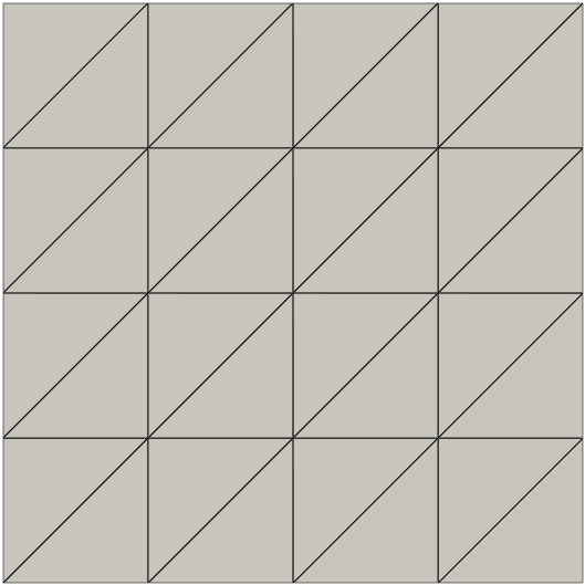
(a) A symmetric, Delaunay mesh.

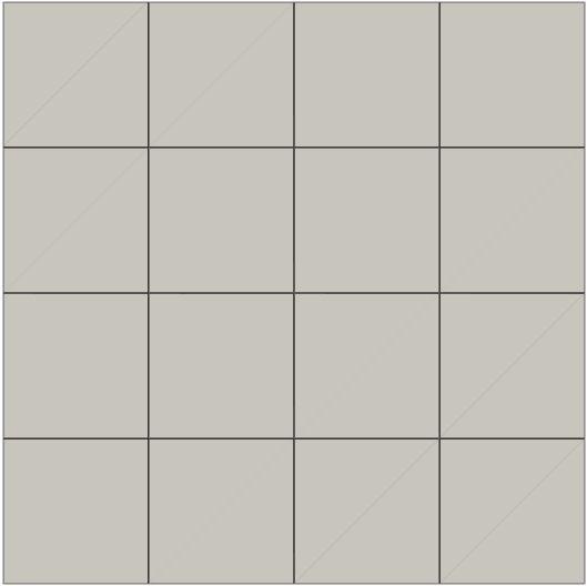
(b) A simple quadrilateral mesh.

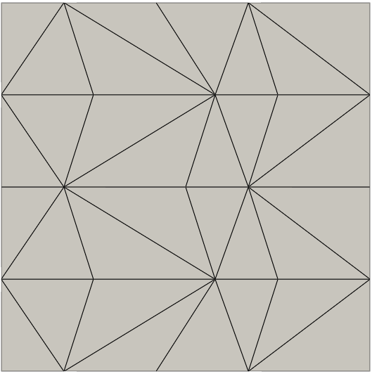
(c) A non-symmetric, non-Delaunay mesh.

Figure 1: Three coarse level indicative meshes used in the experiments all with $N=5$.

To solve the nonlinear problem (28) at each discrete time $t_{n}$, $n=1,2,\ldots,N$, first we set $\tilde{u}^{0}:=u_{h}^{n-1}$. Next, by choosing an appropriate damping parameter $\omega\in(0,1]$ the following fixed point Richardson-like iterative method is used to find $\tilde{u}^{m+1}\in V_{\mathcal{P}}$, such that

$$\left(\tilde{u}^{m+1},v_{h}\right)_{\Omega}+\Delta t\theta a_{J}\left(\tilde{u}^{m+1},v_{h}\right)=\left(\tilde{u}^{m},v_{h}\right)_{\Omega}+\Delta t\theta a_{J}\left(\tilde{u}^{m},v_{h}\right)$$ (55)

$$\hskip 28.45274pt+\omega\left\{F^{n}(v_{h})-\left[\left((\tilde{u}^{m})^{+},v_{h}\right)_{\Omega}+\Delta t\theta a_{J}\left((\tilde{u}^{m})^{+},v_{h}\right)+s\left((\tilde{u}^{m})^{-},v_{h}\right)\right]\right\}\quad\forall v_{h}\in V_{\mathcal{P}},$$

for $m=1,2,\ldots,N_{\textrm{max}}$, or until the following stopping criterion is achieved

$$\parallel\tilde{u}^{m+1}-\tilde{u}^{m}\|_{0,\Omega}\leq 10^{-8}.$$ (56)

Finally, for $m_{0}$ which satisfies in (56), we set $u_{h}^{n}=\tilde{u}^{m_{0}+1}$.

In all figures, $P-1$ indicates the number of divisions in the $x$ and $y$ directions, resulting in a total of $P^{2}$ vertices, including the boundary. We evaluate the method’s asymptotic performance in the $\parallel\cdot\parallel_{0,\Omega}$-norm at the final step, i.e., $\parallel e_{h}^{N}\parallel_{0,\Omega}$, and to verify the result from Theorem 4.4 we examine the asymptotic behaviour of the error by the following norm

$$\parallel e^{N}\parallel_{h}^{2}:=\parallel e^{N}\parallel_{0,\Omega}^{2}+\sum_{n=0}^{N}\Delta t\left(\varepsilon\parallel\nabla e^{n}_{h}\parallel_{0,\Omega}^{2}+\mu\parallel e^{n}_{h}\parallel_{0,\Omega}^{2}+J(e^{n}_{h},e^{n}_{h})\right).$$ (57)

We have used $\mathbb{P}_{1}$ and $\mathbb{P}_{2}$ elements in the triangular meshes, and $\mathbb{Q}_{1}$ elements in the quadrilateral mesh. In the numerical experiments we use the bound preserving Euler (BP-Euler) (44) and the bound preserving Crank-Nicholson (BP-CN), i.e., the method (28) with $\theta=\frac{1}{2}$, even though stability and error estimates for BP-CN has not been proven.

Example 1 (A problem with a smooth solution).

We consider $\mu=1$, $\varepsilon=10^{-6}$, $\boldsymbol{\beta}=(2,1)$, and set $f$ and $u^{0}$ such that the function

$$u(x,y,t)=\exp(t)\sin(\pi x)\sin(\pi y)\,\quad\Omega=(0,1)^{2},$$

is the analytical solution of (2). Notice that $u(x,y,t)\in[0,\exp(t)]$, and thus we set $\kappa(t)=\exp(t)$ as the upper bound at time $t$. The CIP stabilisation parameter $\gamma=0.05$ has been used in (19) and we set $\omega=0.1$ for the damping parameter in all the time steps.

Figure 2 illustrates the asymptotic behaviour of the error $\parallel e_{h}^{N}\parallel_{0,\Omega}$ using $\mathbb{P}_{1}$ and $\mathbb{P}_{2}$ elements. These results align with the theoretical findings we established in Theorem 4.4. By fixing $\Delta t=4\times 10^{-4}$ and decreasing the mesh size as depicted in Figures 2a and 2c, we observe second- and third-order convergence when using $\mathbb{P}_{1}$ and $\mathbb{P}_{2}$ elements, respectively, for both BP-Euler and BP-CN. Also, by fixing the mesh size $h=5\times 10^{-3}$ and varying the length of the time-step $\Delta t$, as shown in Figures 2b and 2d, we obtained first-order convergence for the Euler method and second-order convergence for Crank-Nicholson for both $\mathbb{P}_{1}$ and $\mathbb{P}_{2}$ elements, as expected.

Figure 3 depicts the asymptotic behaviour of the error $\parallel e^{N}\parallel_{h}^{2}$ using $\mathbb{P}_{1}$ and $\mathbb{P}_{2}$ elements. These results also corroborate the theoretical results we proved in Theorem 4.4. By fixing the time step and decreasing the mesh size as shown in Figures 3a and 3c, we observed second- and third-order convergence when using $\mathbb{P}_{1}$ and $\mathbb{P}_{2}$ elements, respectively for the BP-Euler method. This extra order of convergence is, most likely, due to the fact that the small value of $\varepsilon$ makes that the $\|\cdot\|_{h}$ norm is dominated by the $L^{2}(\Omega)$-norm. Additionally, we achieved first-order convergence for the BP-Euler method for both $\mathbb{P}_{1}$ and $\mathbb{P}_{2}$ elements when the size of the time step is decreased. Figures 3b and 3d show the asymptotic behaviour with respect to time for the BP-Euler method.

To assess the computational cost of the nonlinear algorithm at each time step, we depicted in Figure 4 the average number of iterations per step over 1000 time steps for a sequence of meshes with decreasing mesh size. The results indicate that there is no significant increase in the average number of iterations, which remains relatively low regardless of the mesh size.

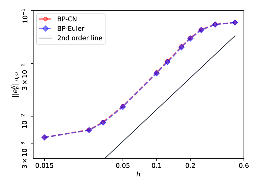
(a) $\Delta t=4\times 10^{-4}$, T=0.2, $\mathbb{P}_{1}$ elements.

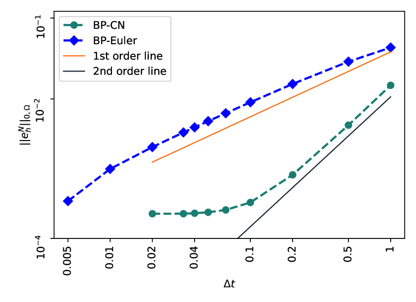
(b) $h=5\times 10^{-3}$, $T=1$, $\mathbb{P}_{1}$ elements.

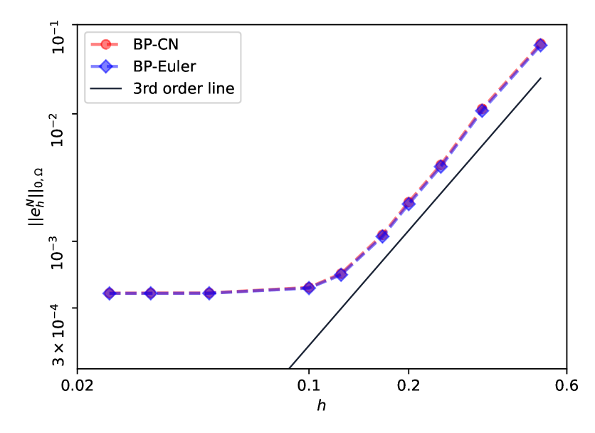
(c) $\Delta t=4\times 10^{-4}$, T=0.2, $\mathbb{P}_{2}$ elements.

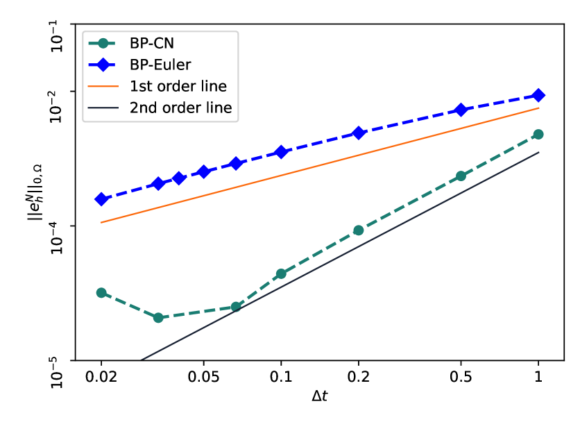
(d) $h=5\times 10^{-3}$, $T=1$, $\mathbb{P}_{2}$ elements

Figure 2: Comparison of the error of the approximated solution by the BP-Euler method and BP-CN method with the exact solution in $\parallel\cdot\parallel_{0,\Omega}$-norm (using mesh 1a).

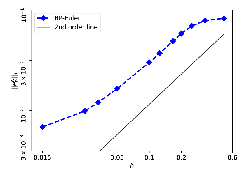
(a) $\Delta t=4\times 10^{-4}$, T=0.2, $\mathbb{P}_{1}$ elements.

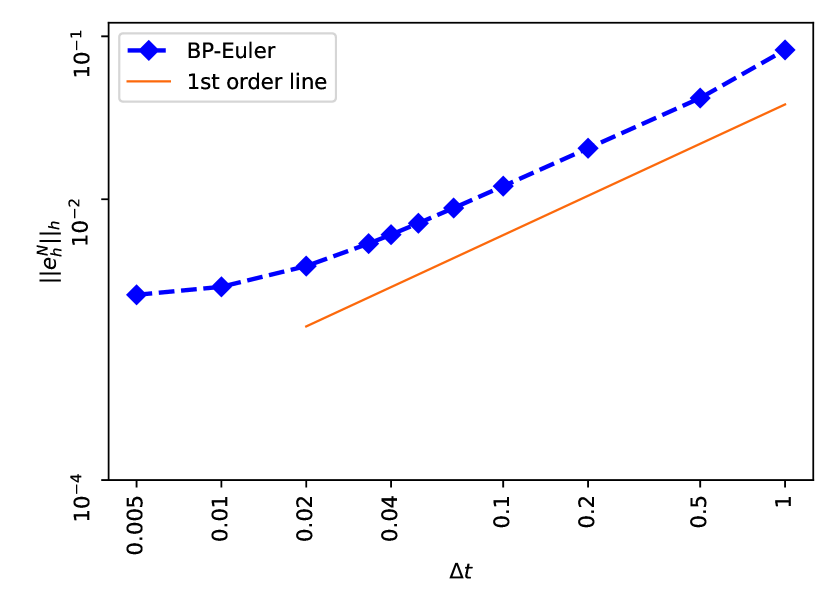
(b) $h=5\times 10^{-3}$, $T=1$, $\mathbb{P}_{1}$ elements.

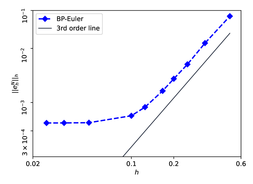
(c) $\Delta t=4\times 10^{-4}$, T=0.2, $\mathbb{P}_{2}$ elements.

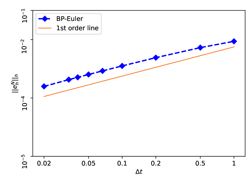
(d) $h=5\times 10^{-3}$, $T=1$, $\mathbb{P}_{2}$ elements

Figure 3: Using norm (57) for the comparison of the error of the approximated solution by the BP-Euler method with the exact solution (using mesh 1a).

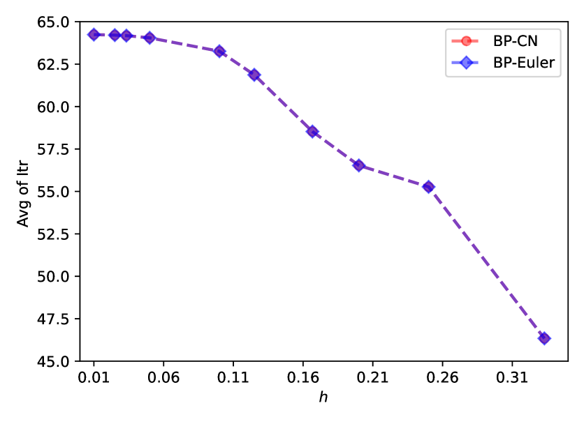
(a) $\mathbb{P}_{1}$ elements

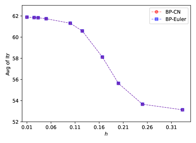
(b) $\mathbb{Q}_{1}$ elements

Figure 4: The average number of the Richardson iterations of 1000 time steps ($T=1$) needed to reach convergence using $\mathbb{P}_{1}$ and $\mathbb{Q}_{1}$ elements and BP-Euler and BP-CN methods and the meshes 1a and 1b.

Example 2 (Three body rotation).

This example is a modified version of the three body rotation transport problem from [27]. We used $\boldsymbol{\beta}=(0.5-y,x-0.5)$, $\varepsilon=10^{-12}$ and $\mu=f=0$. The initial setup involves three separate bodies, as depicted in Figure 5. Each body’s position is defined by its centre at coordinates $(x_{0},y_{0})$. Every body is contained within a circle of radius $r_{0}=0.15$ cantered at $(x_{0},y_{0})$. Outside these three bodies, the initial condition is zero.

Let

$$r(x,y)=\frac{1}{r_{0}}\sqrt{(x-x_{0})^{2}+(y-y_{0})^{2}}.$$ (58)

The center of the slotted cylinder is in $(x_{0},y_{0})=(0.5,0.75)$ and its geometry is given by

$$u(0;x,y)=\left\{\begin{array}[]{ll}1\hskip 8.5359pt{\rm if}\hskip 8.5359ptr(x,y)\leq 1,|x-x_{0}|\geq 0.0225\hskip 8.5359pt{\rm or}y\geq 0.85;\\ 0\hskip 5.69046pt{\rm else},\end{array}\right.$$ (61)

The conical body at the bottom side is described by $(x_{0},y_{0})=(0.5,0.25)$ and

$$u(0;x,y)=1-r(x,y).$$ (62)

Finally, the hump at the left hand side is given by $(x_{0},y_{0})=(0.25,0.5)$ and

$$u(0;x,y)=\frac{1}{4}(1+\cos(\pi\min\{r(x,y),1\})).$$ (63)

The rotation of the bodies occurs counter-clockwise. A full revolution takes $t=2\pi$. We use $P=130$ so a regular grid consisting of $130\times 130$ mesh cells for $\mathbb{P}_{1}$, $\mathbb{P}_{2}$, and $\mathbb{Q}_{1}$ elements.

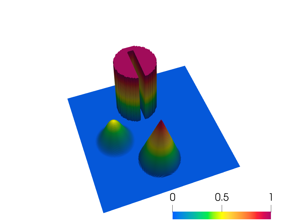
Figure 5: Initial data $u^{0}$ for rotating body problem.

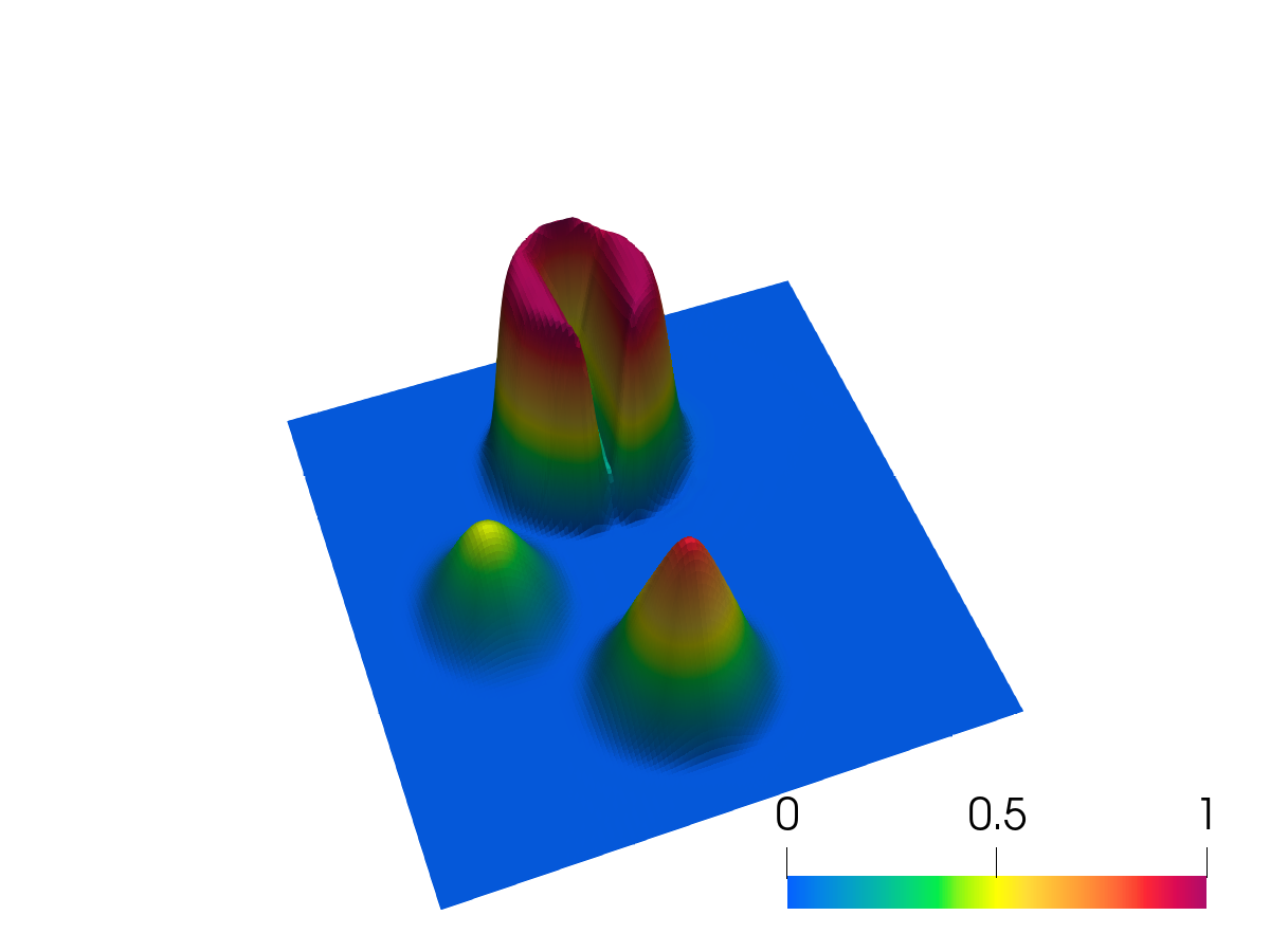
(a) BP-Euler-$\mathbb{P}_{1}$ elements

(b) BP-CN,$\mathbb{P}_{1}$ elements

(c) BP-Euler-$\mathbb{P}_{2}$ elements

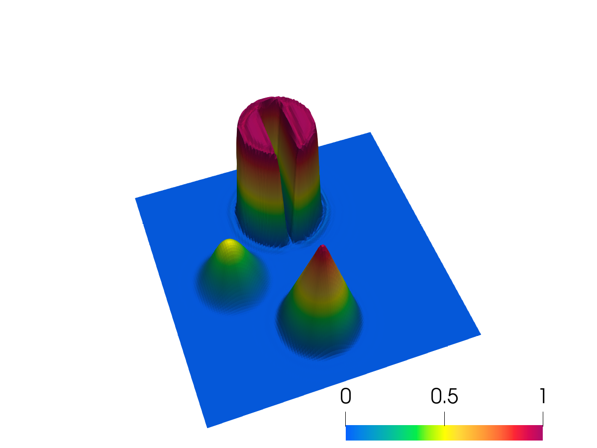
(d) BP-CN-$\mathbb{P}_{2}$ elements

(e) BP-Euler-$\mathbb{Q}_{1}$ elements

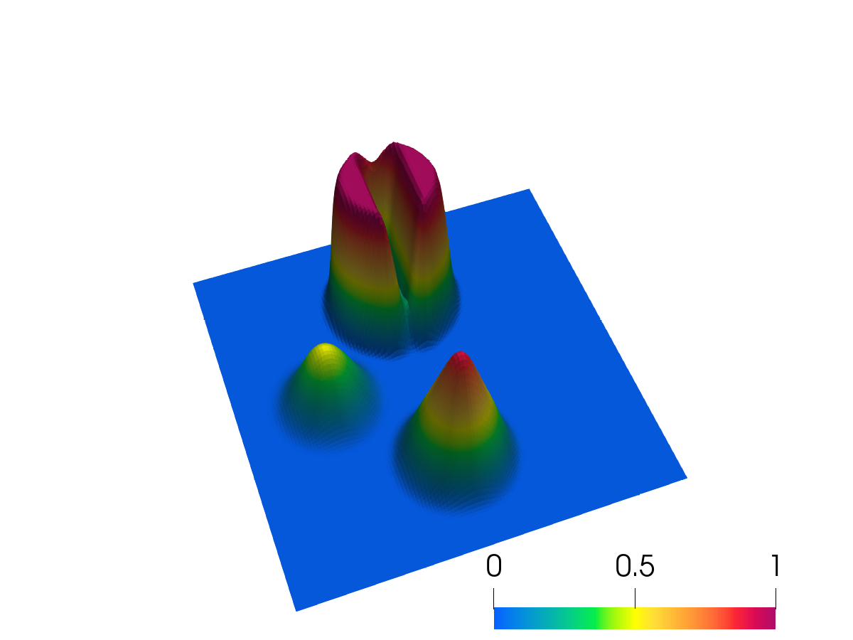
(f) BP-CN-$\mathbb{Q}_{1}$ elements

Figure 6: The approximation of the solution of Example 2 for BP-Euler method and BP-CN method at $T=6.28$ ($\gamma=0.001$, $P=130$).

The simulations were performed with the final time $T=2\pi$ and the time step $\Delta t=10^{-3}$. Figure 6 depicts the approximation solution for the BP-Euler method and BP-CN method using $\mathbb{P}_{1}$, $\mathbb{P}_{2}$ and $\mathbb{Q}_{1}$ elements. In both methods the CIP term (19) was used with the parameter $\gamma=0.001$. Our numerical experiments show that the optimal value of $\omega$ (relative to the number of iterations needed to reach convergence) is approximately $0.07$ when using the quadrilateral mesh, while for $\mathbb{P}_{1}$ and $\mathbb{P}_{2}$ elements, it is around $0.12$. So, we report the results using these values.

For comparison purposes, we also approximated the same problem with CIP-Euler and CIP-Crank-Nicolson (CIP-CN) (the method that only use the CIP term i.e., the full time-space discretisation $\theta$ scheme of the method (20)) with the same value for the parameter $\gamma$. To compare the numerical solution of different methods, a cross section along the line $y=0.75$ was taken of $u^{0}$, BP-Euler, BP-CN, CIP-Euler and CIP-CN methods. The results have been shown in Figure 7. Since we perform a full rotation, we can compare the solution from each method with the initial condition to assess the diffusive properties of each method. As shown in Figure 7, among all the methods, BP-CN demonstrates the best performance regardless of the type of elements used.

Two final experiments are presented. The first aims at assessing the effect of adding CIP stabilization to the method (28). For this, we set $\gamma=0$ in $J(\cdot,\cdot)$ and the results are shown in Figure 8 for the BP-CN method using $\mathbb{P}_{1}$ elements. In Figure 8 we can observe the solution $u_{h}^{+}$, while respecting the bounds of the exact solution, exhibits spurious oscillations near the layers. This justifies the need for CIP stabilization in (28).

To test the performance of the method in the case when the mesh used is not Delaunay, we have approximated this example also in the non-Delaunay mesh depicted in Figure 1c, using $P=130$. The same cross-sections of the approximate solutions for the BP-Euler and BP-CN methods are depicted in Figure 9, alongside the cross-sections for the CIP stabilised finite element method. In both cases $\gamma=0.001$ has been used in the simulation. From the results we can observe, once again, that $u_{h}^{+}$ respects the bounds of Assumption (A1), while the CIP solution presents noticeable over and undershoots.

Finally, to study mass conservation we use the relative mass, i.e. the ratio of the mass at time $t$ to the initial mass defined by

$$M_{r}(t)=\frac{M(t)}{M(0)},$$

where $M(t)$ is the total mass at time $t$, and is defined as

$$M(t)=\int_{\Omega}u(\boldsymbol{x},t)\,\mathrm{d}\boldsymbol{x}.$$

The evolution of mass over time for BP-Euler and BP-CN methods is presented in Figure 10. The plot depicts the evolution of the relative mass. In there, we observe that, despite the fact that the scheme does not preserve mass, the mass loss/gain remains low throughout the simulation.

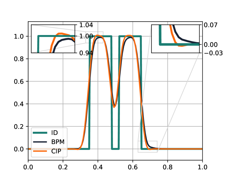
(a) Euler, $\mathbb{P}_{1}$ elements

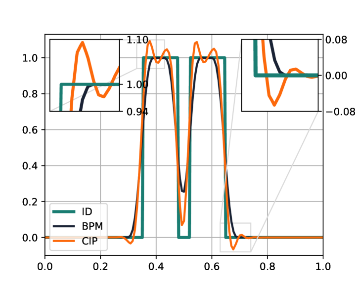
(b) CN, $\mathbb{P}_{1}$ elements

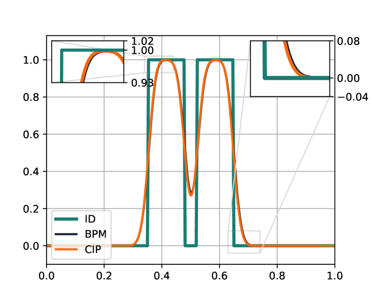
(c) Euler, $\mathbb{P}_{2}$ elements

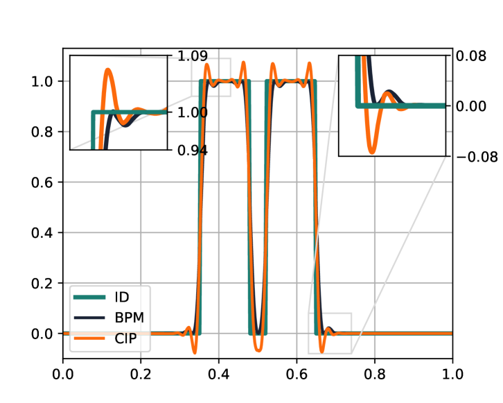
(d) CN, $\mathbb{P}_{2}$ elements

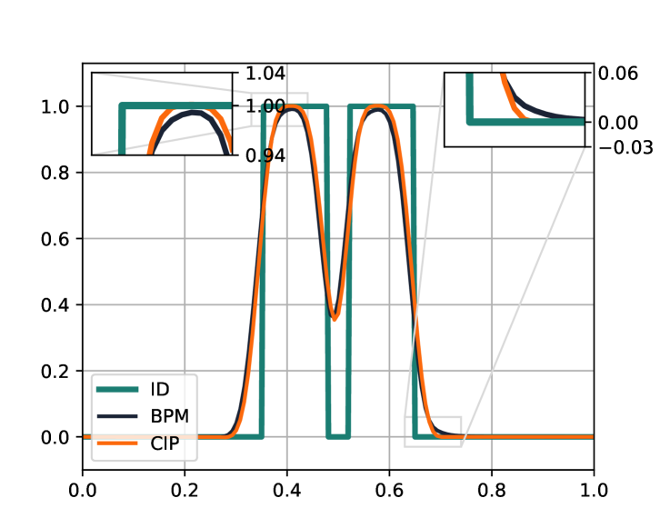
(e) Euler, $\mathbb{Q}_{1}$ elements

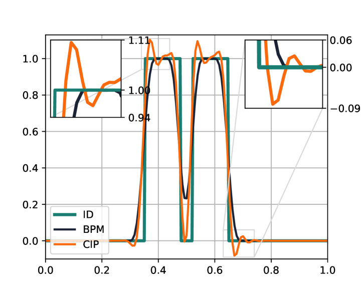
(f) CN, $\mathbb{Q}_{1}$ elements

Figure 7: Cross sections were taken along the line $y=0.75$ of Initial data $u^{0}$, BP-Euler, BP-CN, CIP-Euler and CIP-CN methods at $T=6.28$ ($\gamma=0.001$, $P=130$). For plotting these cross-sections, when $\mathbb{P}_{2}$ elements are used 10,000 equidistant points were chosen along the line $y=0.75$, and the values of the approximated solution have been plotted at these points.

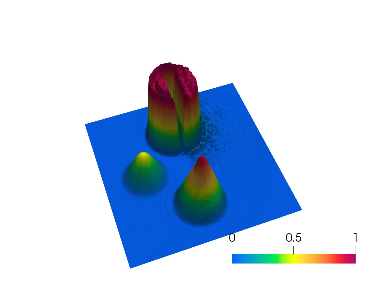
(a) Euler, $\mathbb{P}_{1}$ elements

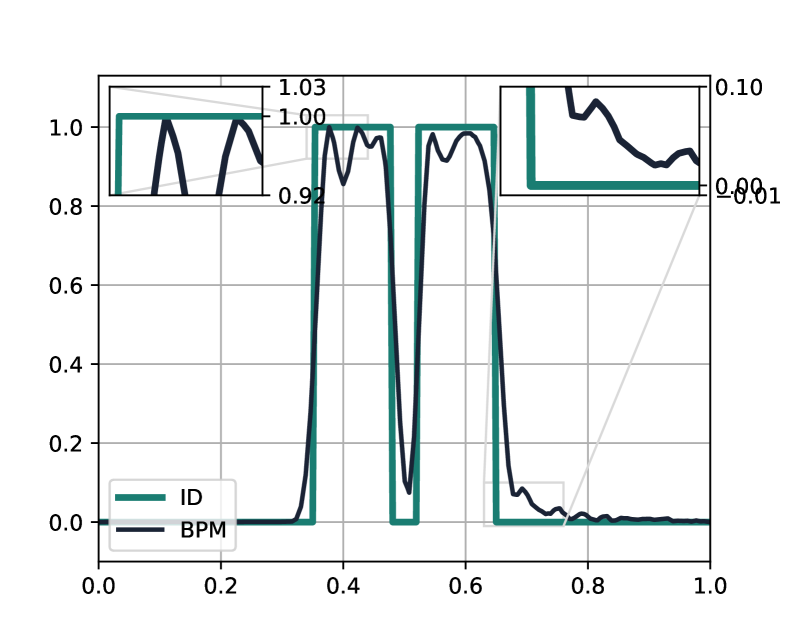
(b) CN, $\mathbb{P}_{1}$ elements

Figure 8: Left: The approximation of the solution of Example 2 for BP-CN method without CIP term ($\gamma=0$) using $\mathbb{P}_{1}$ elements and mesh 1a ($P=130$) Right: Cross sections were taken along the line $y=0.75$ of Initial data $u^{0}$ and BP-CN method without CIP term at $T=6.28$.

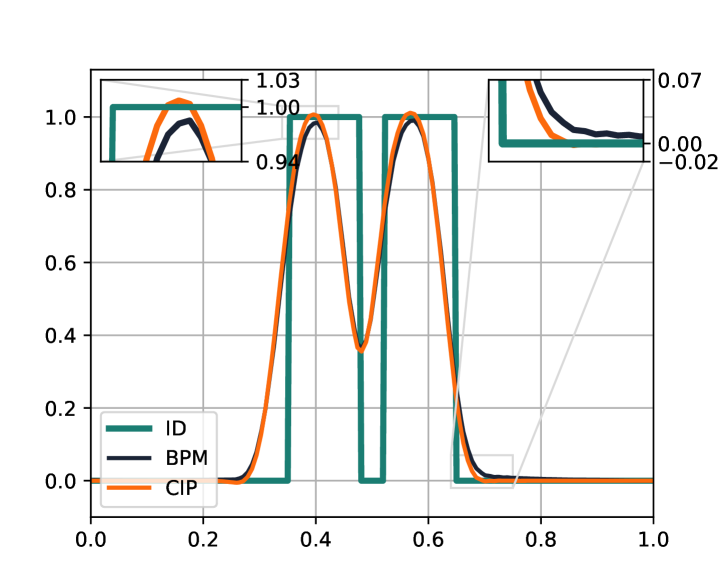
(a) Euler, $\mathbb{P}_{1}$ elements

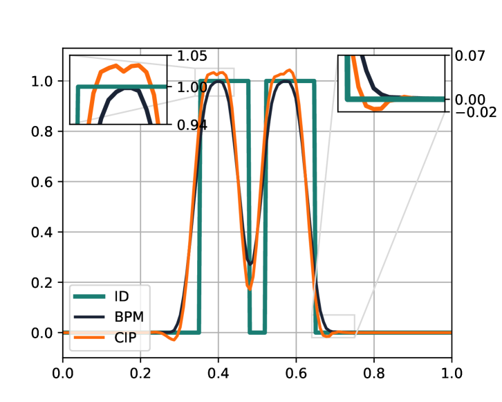
(b) CN, $\mathbb{P}_{1}$ elements

Figure 9: Cross sections were taken along the line $y=0.75$ of Initial data $u^{0}$, BP-Euler, BP-CN, CIP-Euler and CIP-CN methods at $T=6.28$ ($\gamma=0.001$, $P=130$) on the non-Delaunay mesh 1c.

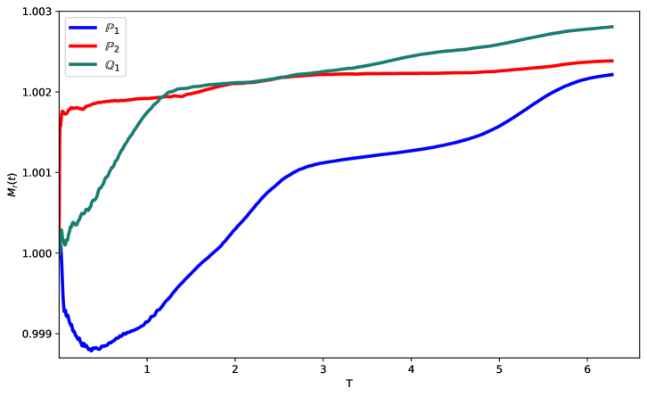
(a) Euler

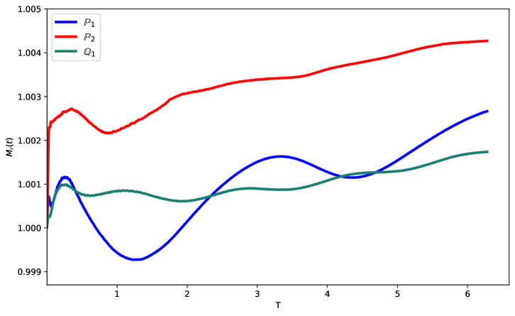
(b) CN

Figure 10: The evolution of mass over time employing the BP-Euler and BP-CN schemes. These methods have been implemented with $\mathbb{P}_{1}$ and $\mathbb{P}_{2}$ elements on Mesh 1a, and $\mathbb{Q}_{1}$ elements on Mesh 1b.

6 Conclusions and outlook

In this work we have build-up on the works [17, 18] and extended that framework to the time-dependent convection-diffusion equation. The analysis of stability and error estimates has been restricted to the implicit Euler scheme, but the method itself has also been tested in the context of the Crank-Nicolson time discretisation. For both options, the numerical experiments show a good performance, with the solution respecting the physical bounds, while at the same time the layers in the solution do not seem to be excessively smeared.

It is important to mention that more economical alternatives, such as linearised flux-corrected transport (FCT) methods (see, e.g., [28]), are also available to ensure bound preservation. Nevertheless, several factors should be considered. One aspect is the CFL condition, as most linear flux-corrected transport methods require such a condition to guarantee bound preservation, whereas our approach does not impose this restriction. Another consideration is the applicability to higher-order elements. FCT methods have primarily been developed for linear finite elements, and bound preservation is not guaranteed for higher-order elements, as the necessary analysis has not yet been carried out. Additionally, improvements to the nonlinear solver itself can enhance performance. In this paper, we used a simple Richardson type solver to highlight the simplicity of the scheme, but more efficient nonlinear solvers, such as localised Newton methods (see, e.g., [29]), or active set methods [30], can significantly improve convergence speed. Our preliminary results indicate that these alternatives provide much faster convergence.

Several problems remain open at this point. The extension of the stability and error analysis to higher-order time discretisation is, at the moment, an open problem. In addition, the extension of this framework to the transport equation is also of interest. A parallel development is the extension of this methodology to discontinuous Galerkin scheme in space, which is the topic of the companion paper [31]. These, and other topics will be the subject of future research.

Acknowledgements

The work of AA, GRB, and TP has been partially supported by the Leverhulme Trust Research Project Grant No. RPG-2021-238. TP is also partially supported by EPRSC grants EP/W026899/2, EP/X017206/1 and EP/X030067/1.

References

-
[1]
A. N. Brooks, T. J. R. Hughes,
Streamline
upwind/Petrov-Galerkin formulations for convection dominated flows with
particular emphasis on the incompressible Navier-Stokes equations,
Comput. Methods Appl. Mech. Engrg. 32 (1-3) (1982) 199–259, fENOMECH ”81,
Part I (Stuttgart, 1981).
doi:10.1016/0045-7825(82)90071-8.
URL https://doi.org/10.1016/0045-7825(82)90071-8 -
[2]
T. J. Hughes, L. P. Franca, G. M. Hulbert,
A
new finite element formulation for computational fluid dynamics: Viii. the
galerkin/least-squares method for advective-diffusive equations, Computer
Methods in Applied Mechanics and Engineering 73 (2) (1989) 173–189.
doi:https://doi.org/10.1016/0045-7825(89)90111-4.
URL https://www.sciencedirect.com/science/article/pii/0045782589901114 -
[3]
E. Burman,
Consistent
SUPG–method for transient transport problems: Stability and
convergence, Computer Methods in Applied Mechanics and Engineering 199 (17)
(2010) 1114–1123.
doi:https://doi.org/10.1016/j.cma.2009.11.023.
URL https://www.sciencedirect.com/science/article/pii/S0045782509003983 -
[4]
P. B. Bochev, M. D. Gunzburger, J. N. Shadid,
Stability
of the SUPG finite element method for transient advection–diffusion
problems, Computer Methods in Applied Mechanics and Engineering 193 (23)
(2004) 2301–2323.
doi:https://doi.org/10.1016/j.cma.2004.01.026.
URL https://www.sciencedirect.com/science/article/pii/S0045782504000830 -
[5]
J.-L. Guermond, Stabilization of
Galerkin approximations of transport equations by subgrid modeling, M2AN
Math. Model. Numer. Anal. 33 (6) (1999) 1293–1316.
doi:10.1051/m2an:1999145.
URL https://doi.org/10.1051/m2an:1999145 -
[6]
E. Burman, P. Hansbo, Edge
stabilization for Galerkin approximations of convection-diffusion-reaction
problems, Comput. Methods Appl. Mech. Engrg. 193 (15-16) (2004) 1437–1453.
doi:10.1016/j.cma.2003.12.032.
URL https://doi.org/10.1016/j.cma.2003.12.032 - [7] R. Becker, M. Braack, A two-level stabilization scheme for the Navier-Stokes equations, in: Numerical mathematics and advanced applications, Springer, Berlin, 2004, pp. 123–130.
-
[8]
E. Burman, M. A. Fernández,
Finite
element methods with symmetric stabilization for the transient
convection–diffusion–reaction equation, Computer Methods in Applied
Mechanics and Engineering 198 (33) (2009) 2508–2519.
doi:https://doi.org/10.1016/j.cma.2009.02.011.
URL https://www.sciencedirect.com/science/article/pii/S0045782509000851 - [9] P. G. Ciarlet, P.-A. Raviart, Maximum principle and uniform convergence for the finite element method, Comput. Methods Appl. Mech. Engrg. 2 (1973) 17–31.
-
[10]
J. Xu, L. Zikatanov, A
monotone finite element scheme for convection-diffusion equations, Math.
Comp. 68 (228) (1999) 1429–1446.
doi:10.1090/S0025-5718-99-01148-5.
URL https://doi.org/10.1090/S0025-5718-99-01148-5 -
[11]
G. R. Barrenechea, V. John, P. Knobloch,
Finite element methods respecting
the discrete maximum principle for convection-diffusion equations, SIAM Rev.
66 (1) (2024) 3–88.
doi:10.1137/22M1488934.
URL https://doi.org/10.1137/22M1488934 - [12] A. Mizukami, T. J. R. Hughes, A Petrov-Galerkin finite element method for convection-dominated flows: an accurate upwinding technique for satisfying the maximum principle, Comput. Methods Appl. Mech. Engrg. 50 (2) (1985) 181–193. doi:10.1016/0045-7825(85)90089-1.
- [13] E. Burman, A. Ern, Stabilized Galerkin approximation of convection-diffusion-reaction equations: discrete maximum principle and convergence, Math. Comp. 74 (252) (2005) 1637–1652 (electronic). doi:10.1090/S0025-5718-05-01761-8.
- [14] D. Kuzmin, Algebraic flux correction for finite element discretizations of coupled systems, in: M. Papadrakakis, E. Oñate, B. Schrefler (Eds.), Proceedings of the Int. Conf. on Computational Methods for Coupled Problems in Science and Engineering, CIMNE, Barcelona, 2007, pp. 1–5.
- [15] G. R. Barrenechea, E. Burman, F. Karakatsani, Edge-based nonlinear diffusion for finite element approximations of convection-diffusion equations and its relation to algebraic flux-correction schemes, Numer. Math. 135 (2) (2017) 521–545.
-
[16]
C. Lu, W. Huang, E. S. Van Vleck,
The
cutoff method for the numerical computation of nonnegative solutions of
parabolic pdes with application to anisotropic diffusion and lubrication-type
equations, Journal of Computational Physics 242 (2013) 24–36.
doi:https://doi.org/10.1016/j.jcp.2013.01.052.
URL https://www.sciencedirect.com/science/article/pii/S0021999113001307 -
[17]
G. R. Barrenechea, E. H. Georgoulis, T. Pryer, A. Veeser,