Mass conservation, positivity and energy identical-relation preserving scheme for the Navier-Stokes equations with variable density

Abstract

In this paper, we consider a mass conservation, positivity and energy identical-relation preserving scheme for the Navier-Stokes equations with variable density. Utilizing the square transformation, we first ensure the positivity of the numerical fluid density, which is form-invariant and regardless of the discrete scheme. Then, by proposing a new recovery technique to eliminate the numerical dissipation of the energy and to balance the loss of the mass when approximating the reformation form, we preserve the original energy identical-relation and mass conservation of the proposed scheme. To the best of our knowledge, this is the first work that can preserve the original energy identical-relation for the Navier-Stokes equations with variable density. Moreover, the error estimates of the considered scheme are derived. Finally, we show some numerical examples to verify the correctness and efficiency.

1 Introduction

In this paper, we focus on the incompressible Navier-Stokes equations with variable density

$$\rho_{t}+\nabla\cdot(\rho u) =0, \mathrm{in}~\Omega\times(0,T],$$ (1.1)

$$\rho u_{t}-\mu\Delta u+\rho(u\cdot\nabla)u+\nabla p =f, \mathrm{in}~\Omega\times(0,T],$$ (1.2)

$$\nabla\cdot u =0, \mathrm{in}~\Omega\times(0,T],$$ (1.3)

where $\Omega\subset\mathcal{R}^{2}$ is a convex polygonal domain with a sufficiently smooth boundary $\partial\Omega$, the density of the fluid is denoted by $\rho=\rho(\mathbf{x},t)$, the velocity of the fluid is represented by $u=(u_{1}(\mathbf{x},t),u_{2}(\mathbf{x},t))^{\top}$, $\mu$ denotes the viscosity coefficient, $f=(f_{1}(\mathbf{x},t),f_{2}(\mathbf{x},t))^{\top}$ is a given function. Moreover, we give the following initial conditions and boundary conditions:

$$\left\{\begin{array}[]{l}\rho(\mathbf{x},0)=\rho_{0}(\mathbf{x}),\\ u(\mathbf{x},0)=u_{0}(\mathbf{x}),\\ \end{array}\right.\left\{\begin{array}[]{l}\rho(\mathbf{x},t)|_{\Gamma_{in}}=a(\mathbf{x},t),\\ u(\mathbf{x},t)|_{\partial\Omega}=g(\mathbf{x},t),\\ \end{array}\right.$$ (1.8)

The functions $\rho_{0}(\mathbf{x})$, $a(\mathbf{x},t)$, $u_{0}(\mathbf{x})$ and $g(\mathbf{x},t)$ are provided, the inflow boundary is defined as $\Gamma_{in}=\{\mathbf{x}\in\partial\Omega:g\cdot\vec{\nu}<0\}$, where $\vec{\nu}$ represents the outward normal vector, and the initial density $\rho_{0}(\mathbf{x})$ satisfy the following conditions [22]

$$0<\rho_{0}^{min}\leq\rho(t,\mathbf{x})\leq\rho_{0}^{max}~~~\mathrm{in}~\Omega.$$ (1.9)

For simplicity, we consider that $g(x,t)=0$ and assume that the boundary $\partial\Omega$ is impervious, which means $g\cdot\vec{\nu}=0$ on $\partial\Omega$ and $\Gamma_{in}=\emptyset$ in this paper. Navier-Stokes equations with variable density (1.1)-(1.3) are a hyperbolic-parabolic coupled nonlinear system, which plays an important role in fluid mechanics.

For the existence and uniqueness of the solutions of Navier-Stokes equations with variable density (1.1)-(1.3), the reader is referred to, e.g., [5, 9, 14, 29]. On the other hand, there have been lots of attentions in developing efficient numerical methods for (1.1)-(1.3), especially in the schemes preserving physical properties. In 1992, Bell et al. [2] first introduced the projection method for variable density issues, they employed the Crank-Nicolson method for temporal discretization, and utilized a standard difference method for spatial discretization. Subsequently, Almgren et al. [1] and Puckett et al. [33] investigated the conservative adaptive projection method and the higher-order projection method for tracking fluid interfaces, respectively. Unlike other traditional algorithms, this method reduces computational costs by solving the discrete pressure variable through the incorporation of a Poisson equation. In [20], a novel time-stepping method was introduced which had been verified by some numerical examples. Additionally, Li et al. in [19] proposed a second-order mixed stabilized finite element method for solving Navier-Stokes equations with variable density. Furthermore, faced with the same issue, Liu and Walkington [23] conducted an investigation into the discontinuous Galerkin (DG) method. They proved the convergence of the scheme but did not provide any convergence rates. In contrast, Pyo and Shen [34] studied two Gauge-Uzawa schemes and demonstrated that the first-order temporally discretized Gauge-Uzawa schemes possess unconditional stability. Moreover, Li and Wu [18] presented a filtered time-stepping technique [6], which could improve the time accuracy to second-order. Afterwards, Reuter et al.[35] introduced a novel algorithm of explicit temporal discretization for low-Mach Navier-Stokes equations with variable density, which achieved second-order accuracy in time. By constructing an implicit temporal scheme with the Taylor series and using a finite element with standard high-order Lagrange basis functions, Lundgren et al. [25] considered a fourth-order method for (1.1)-(1.3).

When designing numerical schemes, one of interesting and challenging topics is to preserve the physical properties of the continuous model at the discrete scheme, which has attracted lots of attentions in the past decade. For the Navier-Stokes equations with constant density, by transforming into an equivalent form known as the EMAC formulation in [4], a mixed finite element method are proposed, which imposed the incompressible condition weakly and preserved physical properties such as momentum, energy, and enstrophy. This research was further extended to address long-term approximations in [28] and three-dimensional problems in [13]. Concurrently, a mimetic spectral element method was introduced in [30], that is capable of preserving mass, energy, enstrophy, and vorticity. Additionally, this concept was adapted to problems involving moving domains in [11]. Lately, by deriving the viscosity coefficients through a residual-based shock-capturing approach, Lundgren et al. [24] presented a novel symmetric and tensor-based viscosity method, which can ensure the conservation of angular momentum and the dissipation of kinetic energy. For the variable density incompressible flows, an entropy-stable scheme was explored in [27] by combining the discontinuous Galerkin method with an artificial compressible approximation. Recognizing the significance of density bounds in numerical simulations, a bound-preserving discontinuous Galerkin method was introduced in [17]. Furthermore, Desmons et al. [7] introduced a generalized high-order momentum preserving scheme, which was acknowledged to be easily implementable utilizing the finite volume method. To ensure the positivity preserving of the density, a square transformation $\rho=\sigma^{2}$ was introduced in [22, 21]. By introducing power-type and exponential-type scalar auxiliary variables to define the system’s energy and to balance the incompressible condition’s influence respectively, Zhang et al. [41] reformulated the Navier-Stokes equations with variable density into an equivalent form and subsequently developed a linear, decoupled, and fully discrete finite element scheme. This scheme preserves the mass, momentum, and modified energy conservation relations. Recently, by introducing a formulation with consistent nonlinear terms, the schemes with the numerical density invariant to global shifts was studied in [26]. And the authors in [16] investigate schemes which could preserve the lower bound of the numerical density and energy inequality under the gravitational force.

But, due to the complex nonlinearities and coupling terms, it is challenging to derive error analysis for numerical methods solving the Navier-Stokes equations with variable density. Under the assumptions that the numerical density is bound and can achieves first order convergence, the author in [8] presented a first-order splitting scheme and deduced its error estimates. Recently, giving up the assumption on the numerical density, Cai et al. [3] derived the error estimate of the backward Euler method applied to the 2D Navier-Stokes equations with variable density, leveraging an error splitting technique and discrete maximal $L^{p}$-regularity. Drawing upon this research, Li and An in [22] presented a novel BDF2 finite element scheme, by utilizing the mini element space to approximate both the velocity and the pressure, and employing the quadratic conforming finite element space to approximate the density. Leveraging a post-processed technique, the authors in [15] demonstrated the convergence order of $O(\tau^{2}+h^{2})$ in $L^{2}$-norm for the numerical density $\rho_{h}^{n}$ and numerical velocity $u_{h}^{n}$. Lately, by rewriting the original system, Pan and Cai in [31] proposed a general BDF2 finite element method preserving the energy inequality and deduced its error analysis. But, there is no literature on error estimates for the fully discrete first-order scheme for the Navier-Stokes equations with variable density, which can preserve the positivity of the numerical density and the original energy identical-relation.

In this paper, we will consider a mass conservation, positivity and energy identical-relation preserving scheme for the Navier-Stokes equations with variable density (1.1)-(1.3). To ensure the positivity of the numerical density, we utilize the square transformation considered in [22, 21] to transform the density sub-equation. Compared to other positivity preserving methods, the method considered here has two mainly advantages: form-invariant and irrelevance of the discrete scheme. Therefore, it is possible to directly adopt other schemes in the references for solving the density sub-equation. But, the mass conservation is lost when approximating this reformation form. To overcome this problem, then we use the recovery technique in [38] to preserve the discrete system’s mass. Moreover, to eliminate the numerical dissipation usually existent in the numerical scheme, we propose a new recovery method, which results that this scheme considered in this paper not only can inherit the mass conservation, positivity, original energy identical-relation from the continuous equations, but also achieve the following convergence order in the $L^{2}$-norm

$$\|\rho(\mathbf{x},t_{n})-\rho_{h}^{n}\|_{L^{2}}^{2}+\|u(\mathbf{x},t_{n})-u_{h}^{n}\|_{L^{2}}^{2}\leq C(\tau^{2}+h^{4}),$$

where $C$ is a general positive constant, $h$ and $\tau$ are the spatial mesh size and the temporal step, respectively.

The rest of this paper is organized as follows. In Section 2, we introduce some preliminaries, such as functional spaces, some inequalities commonly used, and an equivalent model with some essential properties. Then, based on this equivalent form, we propose a fully discrete first order recovery finite element scheme in Section 3, that keeps density positivity, mass conversation, and energy identical-relation preserving. Subsequently, in Section 4, we derive the error estimates of the proposed scheme. Furthermore, in Section 5, we present some examples to confirm the convergence orders and efficiency of the recovery finite element scheme. Finally, a conclusion remark is made in Section 6.

2 Preliminaries

In this section, after introducing some functional spaces in the first subsection, we will recall some frequently used inequalities and present some essential properties for the Navier-Stokes equations with variable density in Subsections 2.2 and 2.3, respectively.

2.1 Functional spaces

For $k\in N^{+}$ and $1\leq p\leq+\infty$, we denote $L^{p}(\Omega)$ and $W^{k,p}(\Omega)$ as the classical Lebesgue space and Sobolev space, respectively. The norms of these spaces are denoted by

$$||u||_{L^{p}(\Omega)} =\left(\int_{\Omega}|u(\mathbf{x})|^{p}\,\mathrm{d}x\right)^{\frac{1}{p}},$$

$$||u||_{W^{k,p}(\Omega)} =\left(\sum\limits_{|j|\leq k}||D^{j}u||_{L^{p}(\Omega)}^{p}\right)^{\frac{1}{p}}.$$

Within this context, $W^{k,2}(\Omega)$ is also known as the Hilbert space and can be expressed as $H^{k}(\Omega)$. $||\cdot||_{L^{\infty}}$ represent the norm of space of $L^{\infty}(\Omega)$,

$$||u||_{L^{\infty}(\Omega)}=ess\sup\limits_{\mathbf{x}\in\Omega}|u(\mathbf{x})|,$$

and $(\cdot,\cdot)$ denotes the inner product in $L^{2}(\Omega)$. Furthermore, we define the following frequently utilized mathematical frameworks:

$$W=H^{1}(\Omega),\quad V=(H_{0}^{1}(\Omega))^{2},\quad V_{0}=\{v\in V,\nabla\cdot v=0\},$$

$$M=L_{0}^{2}(\Omega)=\{q\in L^{2}(\Omega),\int_{\Omega}qd\mathbf{x}=0\}.$$

On the other hand, let $\mathcal{T}_{h}=\{K\}$ be a uniformly regular triangulation partition of $\Omega$ with a mesh size $h(0<h<1)$. We also define the finite element space

$$V_{h}=\{u_{h}\in C(\bar{\Omega})\cap V,~v_{h}|_{K}\in P_{2}(K)^{2},~\forall K\in\mathcal{T}_{h}\}\subset V,$$

$$M_{h}=\{p_{h}\in C(\bar{\Omega})\cap H^{1}(\Omega),~q_{h}|_{K}\in P_{1}(K),~\forall K\in\mathcal{T}_{h},~\int_{\Omega}q_{h}d\mathbf{x}=0\}\subset M,$$

$$W_{h}=\{\rho_{h}\in C(\bar{\Omega})\cap W,~r_{h}|_{K}\in P_{2}(K),~\forall K\in\mathcal{T}_{h}\}\subset W,$$

where $P_{m}(K)$ denotes the polynomial space with degree up to $m$ on every triangle $K\in\mathcal{T}_{h}$.

2.2 Some inequalities

We recall some useful inequalities in two dimension in this subsection. For any $v_{h}$ belongs to the finite element space defined above, there hold

1. Inverse inequality [42]:

$$||v_{h}||_{L^{3}} \leq Ch^{-\frac{1}{3}}||v_{h}||_{L^{2}},$$ (2.1)

$$||v_{h}||_{L^{\infty}} \leq Ch^{-1}||v_{h}||_{L^{2}},$$ (2.2)

$$||v_{h}||_{H^{1}} \leq Ch^{-1}||v_{h}||_{L^{2}};$$ (2.3)

2. Agmon’s inequality [10]:

$$||v_{h}||_{L^{\infty}}\leq C||v_{h}||_{L^{2}}^{\frac{1}{2}}||\triangle v_{h}||_{L^{2}}^{\frac{1}{2}}.$$ (2.4)

The famous Gronwall lemma which is frequently used for the time dependent problem is as follows:

Lemma 2.1.

(Gronwall inequality [22]) Let $B>0$ and $a_{k},b_{k},c_{k}$ be non-negative numbers such that

$$a_{n}+\tau\sum\limits_{k=0}^{n}b_{k}\leq\tau\sum\limits_{k=0}^{n}c_{k}a_{k}+B,~n\geq 0.$$ (2.5)

If $\tau c_{k}<1$ and $d_{k}=(1-\tau c_{k})^{-1}$, then there holds

$$a_{n}+\tau\sum\limits_{k=0}^{n}b_{k}\leq\exp\left(\tau\sum\limits_{k=0}^{n}c_{k}d_{k}\right)B,~n\geq 0.$$ (2.6)

Moreover, recalling the $L^{2}$ projection operator $\Pi_{h}$ [22]: $W\rightarrow W_{h}$

$$(\Pi_{h}\sigma-\sigma,r_{h})=0,~\forall r_{h}\in W_{h},$$ (2.7)

and the Stokes projection $(R_{h},Q_{h}):V\times M\rightarrow V_{h}\times M_{h}$

$$(\nabla(R_{h}u-u),\nabla v_{h})-(\nabla\cdot v_{h},Q_{h}p-p) =0,~\forall v_{h}\in V_{h},$$ (2.8)

$$(\nabla\cdot(R_{h}u-u),q_{h}) =0,~\forall q_{h}\in M_{h},$$ (2.9)

we have [22]

$$||u-R_{h}u||_{L^{2}} +h||\nabla(u-R_{h}u)||_{L^{2}}+h||p^{n}-Q_{h}p||_{L^{2}}$$

$$\leq Ch^{3}(||u||_{H^{3}}+||p||_{H^{2}}),$$ (2.10)

$$||\sigma\!-\!\Pi_{h}\sigma||\!_{L^{2}}\! +\!||\rho\!-\!\Pi_{h}\rho||\!_{L^{2}}\!+\!h(||\sigma\!-\!\Pi_{h}\sigma||\!_{H^{1}}\!+\!||\rho\!-\!\Pi_{h}\rho||\!_{H^{1}})\!$$

$$\leq\!Ch^{3}(||\sigma||_{H^{3}}+||\rho||_{H^{2}}).$$ (2.11)

Lemma 2.2.

([37], Theorem 4.4.20) Set $\mathcal{T}_{h}(0<h<1)$ is a nondegenerate subdivision of a polyhedra region $\Omega$. For all $K\in\mathcal{T}_{h}$, $0<h<1$, $\exists C,n,m,p$ so that for $0\leq s\leq m$, there is a global interpolation operator $I_{h}$, which satisfies

$$\left(\sum\limits_{K\in\mathcal{T}_{h}}||v-I_{h}v||_{W_{p}^{s}(K)}^{p}\right)^{\frac{1}{p}}\leq Ch^{m-s}|v|_{W_{p}^{m}(\Omega)}.$$ (2.12)

2.3 Some essential properties

For the Navier-Stokes equations with variable density (1.1)-(1.3), there hold the following essential properties (see [41]):

1. Positivity:

$$\rho(\mathbf{x},t)>0.$$

2. Mass conservation:

$$\int_{\Omega}\rho(\mathbf{x},t)\,\mathrm{d}\mathbf{x}=\int_{\Omega}\rho(\mathbf{x},0)\,\mathrm{d}\mathbf{x}.$$

3. Energy identical-relation:

$$\frac{dE(\rho,u)}{dt}=-\mu\int_{\Omega}|\nabla u|^{2}\,\mathrm{d}\mathbf{x}+\int_{\Omega}fu\,\mathrm{d}\mathbf{x},$$

where the energy $E$ is defined by

$$E=\frac{1}{2}\int_{\Omega}\rho|u|^{2}\,\mathrm{d}\mathbf{x}.$$

When designing numerical schemes for solving the Navier-Stokes equations with variable density (1.1)-(1.3), it is important to ensure them to preserve the above properties, which will improve the computational accuracy.

To preserve the positivity, we adopt the square transformation [21]

$$\rho(\mathbf{x},t)=(\sigma(\mathbf{x},t))^{2},$$ (2.13)

which guarantees that the density is non-negative regardless of the discrete scheme. Moreover, we can derive an equivalent formulation of the continuous equation below

$$\sigma_{t}+\nabla\cdot(\sigma u) =0, \mathrm{in}~\Omega\times(0,T],$$ (2.14)

$$\sigma(\sigma u)_{t}-\mu\triangle u+\rho(u\cdot\nabla)u+\frac{u}{2}\nabla\cdot(\rho u)+\nabla p =f, \mathrm{in}~\Omega\times(0,T],$$ (2.15)

$$\nabla\cdot u =0, \mathrm{in}~\Omega\times(0,T].$$ (2.16)

We can see that the equation (1.1) is form-invariant for this transformation, and the initial data satisfies

$$\sigma_{0}(\mathbf{x})=\sqrt{\rho_{0}(\mathbf{x})}\quad\mathrm{and}\quad\sqrt{\rho_{0}^{min}}\leq\sigma(t,\mathbf{x})\leq\sqrt{\rho_{0}^{max}},\quad~\mathrm{in}~\Omega,$$ (2.17)

by cooperating with (1.9) and the positivity of the density.

Furthermore, to derive the error estimate in the subsequent section, we make the following assumptions on the solutions of the continuous model.

Assumption 2.1.

The solution of (2.14)-(2.16) satisfies the following regularities [21, 22]:

$$\sigma \in C([0,T];H^{3}(\Omega)),~~~~\sigma_{t}\in L^{\infty}([0,T];H^{1}(\Omega))\cap L^{2}([0,T];H^{2}(\Omega)),$$

$$\rho \in C([0,T];H^{3}(\Omega))\cap C^{1}([0,T];H^{2}(\Omega)),$$

$$u \in C([0,T];H^{3}(\Omega))\cap C^{1}([0,T];H^{2}(\Omega)),~~~~p\in C([0,T];H^{2}(\Omega)).$$

3 Property-preserving scheme

In this section, based on a new recovery technique, we will propose a fully discrete first order finite element scheme for solving the incompressible Navier-Stokes equations with variable density. Let $N\in\mathbb{N}^{+}$ and $\tau=T/N(0<\tau<1)$, thus $0=t_{0}<t_{1}<\dots<t_{k}<t_{k+1}\dots<t_{N}=T$. Define $D_{\tau}g^{n+1}:=\frac{g^{n+1}-g^{n}}{\tau}$, then the first order scheme considered in this paper is as follows: Given $(\sigma_{h}^{0},\rho_{h}^{0},u_{h}^{0},p_{h}^{0})=(\Pi_{h}\sigma^{0},\Pi_{h}\rho^{0},R_{h}u^{0},Q_{h}p^{0})$, find $(\sigma_{h}^{n+1},\tilde{u}_{h}^{n+1},p_{h}^{n+1},u_{h}^{n+1},\rho_{h}^{n+1})$ for $0\leq n\leq N-1$ through the following steps:

Step 1. Find $\sigma_{h}^{n+1}\in W_{h}$ such that

$$(D_{\tau}\sigma_{h}^{n+1},r_{h})+(\nabla\sigma_{h}^{n+1}\cdot u_{h}^{n},r_{h})+\frac{1}{2}(\sigma_{h}^{n+1}\nabla\cdot u_{h}^{n},r_{h})=0;$$ (3.1)

Step 2. Find $(\tilde{u}_{h}^{n+1},p_{h}^{n+1})\in(V_{h},M_{h})$ such that

$$(\sigma_{h}^{n+1}D_{\tau}(\sigma_{h}^{n+1}\tilde{u}_{h}^{n+1}),v_{h})+\mu(\nabla\tilde{u}_{h}^{n+1},\nabla v_{h})+(\rho_{h}^{n}(u_{h}^{n}\cdot\nabla)\tilde{u}_{h}^{n+1},v_{h})$$ (3.2)

$$+\frac{1}{2}(\tilde{u}_{h}^{n+1}\nabla\cdot(\rho_{h}^{n}u_{h}^{n}),v_{h})-(p_{h}^{n+1},\nabla\cdot v_{h})+(\nabla\cdot\tilde{u}_{h}^{n+1},q_{h})=(f^{n+1},v_{h});$$

Step 3. Find $u_{h}^{n+1}\in V_{h}$ by

$$u_{h}^{n+1}=\sqrt{\gamma_{h}^{n+1}}\tilde{u}_{h}^{n+1},$$ (3.3)

where

$$\gamma_{h}^{n+1}=\left\{\begin{aligned} &1+\frac{||\sigma_{h}^{n+1}\tilde{u}_{h}^{n+1}-\sigma_{h}^{n}\tilde{u}_{h}^{n}||_{L^{2}}^{2}-||\sigma_{h}^{n}\tilde{u}_{h}^{n}||_{L^{2}}^{2}+||\sigma_{h}^{n}u_{h}^{n}||_{L^{2}}^{2}}{||\sigma_{h}^{n+1}\tilde{u}_{h}^{n+1}||_{L^{2}}^{2}},&||\sigma_{h}^{n+1}\tilde{u}_{h}^{n+1}||_{L^{2}}\neq 0\\ &1,&||\sigma_{h}^{n+1}\tilde{u}_{h}^{n+1}||_{L^{2}}=0\end{aligned};\right.$$ (3.4)

Step 4. Find $\rho_{h}^{n+1}\in W_{h}$ by

$$\rho_{h}^{n+1}=\lambda_{h}^{n+1}\bar{\rho}_{h}^{n+1},\\$$ (3.5)

where

$$\bar{\rho}_{h}^{n+1} =(\sigma_{h}^{n+1})^{2},$$ (3.6)

$$\lambda_{h}^{n+1} =\frac{\int_{\Omega}\rho_{h}^{n}\,\mathrm{d}\mathbf{x}}{\int_{\Omega}\bar{\rho}_{h}^{n+1}\,\mathrm{d}\mathbf{x}}.$$ (3.7)

In Steps 1-2, we get the approximation solutions $\sigma_{h}^{n+1},~\tilde{u}_{h}^{n+1}$ and $p_{h}^{n+1}$ by solving two linear system. But, the mass conservation and the original energy identical-relation is lost in Steps 1 and 2, respectively. To make these numerical solutions to satisfy the property of the continuous equations, we recover them in Steps 3-4, which are made up of several assignment operations and can be implemented efficiently. For the scheme (3.1)-(3.7), there hold the following Theorem.

Theorem 3.1.

The scheme (3.1)-(3.7) inherits the following physical properties of the continuous equations (1.1)-(1.3):

1. Positivity: $\rho_{h}^{n+1}=\lambda_{h}^{n+1}\bar{\rho}_{h}^{n+1}>0$.

2. Mass conservation: $\int_{\Omega}\rho_{h}^{n+1}\,\mathrm{d}\mathbf{x}=\int_{\Omega}\rho_{h}^{n}\,\mathrm{d}\mathbf{x}=\int_{\Omega}\rho_{h}^{0}\,\mathrm{d}\mathbf{x}$.

3. Energy identical-relation:

$$D_{\tau}E^{n+1}=-\mu\int_{\Omega}|\nabla\tilde{u}_{h}^{n+1}|^{2}\,\mathrm{d}\mathbf{x}+\int_{\Omega}f^{n+1}\tilde{u}_{h}^{n+1}\,\mathrm{d}\mathbf{x},$$

where the energy $E^{n+1}$ is defined by:

$$E^{n+1}=\frac{1}{2}||\sigma_{h}^{n+1}u_{h}^{n+1}||_{L^{2}}^{2}.$$

Proof.

The positivity of $\rho_{h}^{n+1}$ can be easily derived by combining the induction method with (3.6)-(3.7).

Then, using (3.6) and (3.7), we can deduce that mass conservation

$$\int_{\Omega}\rho_{h}^{n+1}\,\mathrm{d}\mathbf{x}=\int_{\Omega}\lambda^{n+1}\bar{\rho}_{h}^{n+1}\,\mathrm{d}\mathbf{x}=\int_{\Omega}\rho_{h}^{n}\,\mathrm{d}\mathbf{x}.$$

Finally, taking $(v_{h},q_{h})=(\tilde{u}_{h}^{n+1},p_{h}^{n+1})$ on (3.2), we can get

$$(D_{\tau}(\sigma_{h}^{n+1}\tilde{u}_{h}^{n+1}),\sigma_{h}^{n+1}\tilde{u}_{h}^{n+1})+\mu\int_{\Omega}|\nabla\tilde{u}_{h}^{n+1}|^{2}\,\mathrm{d}\mathbf{x}=\int_{\Omega}f^{n+1}\tilde{u}_{h}^{n+1}\,\mathrm{d}\mathbf{x}.$$

Due to (3.3) and (3.4), $(D_{\tau}(\sigma_{h}^{n+1}\tilde{u}_{h}^{n+1}),\sigma_{h}^{n+1}\tilde{u}_{h}^{n+1})$ can be expressed as follows:

$$(D_{\tau}(\sigma_{h}^{n+1}\tilde{u}_{h}^{n+1}),\sigma_{h}^{n+1}\tilde{u}_{h}^{n+1})$$ (3.8)

$$=\frac{||\sigma_{h}^{n+1}\tilde{u}_{h}^{n+1}||_{L^{2}}^{2}-||\sigma_{h}^{n}\tilde{u}_{h}^{n}||_{L^{2}}^{2}+||\sigma_{h}^{n+1}\tilde{u}_{h}^{n+1}-\sigma_{h}^{n}\tilde{u}_{h}^{n}||_{L^{2}}^{2}}{2\tau}$$

$$=\frac{\gamma_{h}^{n+1}||\sigma_{h}^{n+1}\tilde{u}_{h}^{n+1}||_{L^{2}}^{2}-||\sigma_{h}^{n}u_{h}^{n}||_{L^{2}}^{2}}{2\tau}.$$

Next, we will prove $\gamma_{h}^{n+1}>0$ by using the induction method. Since the result is obvious when $||\sigma_{h}^{n+1}\tilde{u}_{h}^{n+1}||_{L^{2}}=0$, we only consider the case $||\sigma_{h}^{n+1}\tilde{u}_{h}^{n+1}||_{L^{2}}\neq 0$ in the following.

(I) When $n=0$, thanks to $\tilde{u}_{h}^{0}=u_{h}^{0}$, it yields $\gamma_{h}^{1}=1+\frac{||\sigma_{h}^{1}\tilde{u}_{h}^{1}-\sigma_{h}^{0}\tilde{u}_{h}^{0}||_{L^{2}}^{2}}{||\sigma_{h}^{1}\tilde{u}_{h}^{1}||_{L^{2}}^{2}}>0$.

(II) Assume $\gamma_{h}^{m}>0$ for all $1\leq m\leq N-1$. Summing over $n$ from $0$ to $m$ in (3.8) and utilizing (3.3), we can get

$$||\sigma_{h}^{m+1}\tilde{u}_{h}^{m+1}||_{L^{2}}^{2}-||\sigma_{h}^{0}\tilde{u}_{h}^{0}||_{L^{2}}^{2}+\sum\limits_{i=0}^{m}||\sigma_{h}^{i+1}\tilde{u}_{h}^{i+1}-\sigma_{h}^{i}\tilde{u}_{h}^{i}||_{L^{2}}^{2}$$

$$=\gamma_{h}^{m+1}||\sigma_{h}^{m+1}\tilde{u}_{h}^{m+1}||_{L^{2}}^{2}-||\sigma_{h}^{0}u_{h}^{0}||_{L^{2}}^{2},$$

which implies, by noting $\tilde{u}_{h}^{0}=u_{h}^{0}$ again, that

$$\gamma_{h}^{m+1}=1+\frac{\sum\limits_{i=0}^{m}||\sigma_{h}^{i+1}\tilde{u}_{h}^{i+1}-\sigma_{h}^{i}\tilde{u}_{h}^{i}||_{L^{2}}^{2}}{||\sigma_{h}^{m+1}\tilde{u}_{h}^{m+1}||_{L^{2}}^{2}}>0.$$

Therefore, it always holds $\gamma_{h}^{n+1}>0$ for all $0\leq n\leq N-1$. It follows by combining with (3.8) that

$$(D_{\tau}(\sigma_{h}^{n+1}\tilde{u}_{h}^{n+1}),\sigma_{h}^{n+1}\tilde{u}_{h}^{n+1}) =\frac{||\sigma_{h}^{n+1}\sqrt{\gamma_{h}^{n+1}}\tilde{u}_{h}^{n+1}||_{L^{2}}^{2}-||\sigma_{h}^{n}u_{h}^{n}||_{L^{2}}^{2}}{2\tau}$$

$$=\frac{||\sigma_{h}^{n+1}u_{h}^{n+1}||_{L^{2}}^{2}-||\sigma_{h}^{n}u_{h}^{n}||_{L^{2}}^{2}}{2\tau}$$

$$=D_{\tau}E^{n+1},$$

which indicates the original energy identical-relation. The proof is completed. ∎

4 Error estimate

In this section, we will deduce the error estimate of the scheme (3.1)-(3.7). Firstly, from the definitions of the initial data and properties of the projections presented in Section 2, we have the following results for the initial data in the scheme

$$||\sigma(t_{0})-\sigma_{h}^{0}||_{L^{2}}^{2}+||\rho(t_{0})-\rho_{h}^{0}||_{L^{2}}^{2}+||u(t_{0})-u_{h}^{0}||_{L^{2}}^{2}+||p(t_{0})-p_{h}^{0}||_{L^{2}}^{2}\leq C(\tau^{2}+h^{4}).$$ (4.1)

Then, for simplicity, we write $\sigma^{n}=\sigma(t_{n},\mathbf{x}),u^{n}=u(t_{n},\mathbf{x}),\rho^{n}=\rho(t_{n},\mathbf{x}),p^{n}=p(t_{n},\mathbf{x})$ as exact solution. According to the $L^{2}$ projection and Stokes projection recalled in Section 2, we can split the errors as

$$e_{\sigma h}^{n} =\sigma^{n}-\sigma_{h}^{n}=(\sigma^{n}-\Pi_{h}\sigma^{n})+(\Pi_{h}\sigma^{n}-\sigma_{h}^{n}):=\eta_{\sigma h}^{n}+\theta_{\sigma h}^{n},$$

$$\bar{e}_{\rho h}^{n} =\rho^{n}-\bar{\rho}_{h}^{n}=(\rho^{n}-\Pi_{h}\rho^{n})+(\Pi_{h}\rho^{n}-\bar{\rho}_{h}^{n}):=\eta_{\rho h}^{n}+\bar{\theta}_{\rho h}^{n},$$

$$e_{\rho h}^{n} =\rho^{n}-\rho_{h}^{n}=(\rho^{n}-\Pi_{h}\rho^{n})+(\Pi_{h}\rho^{n}-\rho_{h}^{n}):=\eta_{\rho h}^{n}+\theta_{\rho h}^{n},$$

$$\tilde{e}_{uh}^{n} =u^{n}-\tilde{u}_{h}^{n}=(u^{n}-R_{h}u^{n})+(R_{h}u^{n}-\tilde{u}_{h}^{n}):=\eta_{uh}^{n}+\tilde{\theta}_{uh}^{n},$$

$$e_{uh}^{n} =u^{n}-u_{h}^{n}=(u^{n}-R_{h}u^{n})+(R_{h}u^{n}-u_{h}^{n}):=\eta_{uh}^{n}+\theta_{uh}^{n},$$

$$e_{ph}^{n} =p^{n}-p_{h}^{n}=(p^{n}-Q_{h}p^{n})+(Q_{h}p^{n}-p_{h}^{n}):=\eta_{ph}^{n}+\theta_{ph}^{n}.$$

On the other hand, from (2.14)-(2.15), we can derive

$$(D_{\tau}\sigma^{n+1},r)+(\nabla\sigma^{n+1}\cdot u^{n},r)+\frac{1}{2}(\sigma^{n+1}\nabla\cdot u^{n},r)=(R_{\sigma 1}^{n+1},r),~~\forall r\in W,$$ (4.2)

and

$$(\sigma^{n+1}D_{\tau}(\sigma^{n+1}u^{n+1}),v)+\mu(\nabla u^{n+1},\nabla v)+(\rho^{n}(u^{n}\cdot\nabla)u^{n+1},v)$$ (4.3)

$$+\frac{1}{2}(u^{n+1}\nabla\cdot(\rho^{n}u^{n}),v)-(\nabla\cdot v,p^{n+1})+(\nabla\cdot u^{n+1},q)$$

$$=(f^{n+1},v)+(R_{u1}^{n+1},v),~~\forall(v,q)\in V\times M,$$

where

$$R_{\sigma 1}^{n+1} =D_{\tau}\sigma^{n+1}-\sigma_{t}^{n+1}+\nabla\sigma^{n+1}(u^{n}-u^{n+1}),$$

$$R_{u1}^{n+1} =\sigma^{n+1}D_{\tau}(\sigma^{n+1}u^{n+1})-\sigma^{n+1}(\sigma u)_{t}(t_{n+1})+(\rho^{n}-\rho^{n+1})(u^{n}\cdot\nabla)u^{n+1}$$

$$+\rho^{n+1}((u^{n}-u^{n+1})\cdot\nabla)u^{n+1}+\frac{u^{n+1}}{2}\nabla\cdot((\rho^{n}-\rho^{n+1})u^{n})$$

$$+\frac{u^{n+1}}{2}\nabla\cdot(\rho^{n+1}(u^{n}-u^{n+1})).$$

For the above two truncation errors, there holds the following convergence order.

Lemma 4.1.

Under Assumption 2.1, it is valid that

$$\tau\sum\limits_{n=0}^{N-1}(||R_{\sigma 1}^{n+1}||_{L^{2}}^{2}+||R_{u1}^{n+1}||_{L^{2}}^{2})\leq C\tau^{2}.$$ (4.4)

Proof.

By the Taylor’s expansion, we can easily get

$$D_{\tau}g^{n+1}-g_{t}(t_{n+1})=O(\tau),$$ (4.5)

for any smooth enough function $g$. Based on the expressions for $R_{\sigma 1}^{n+1}$ and $R_{u1}^{n+1}$, along with (4.5) and Assumption 2.1, we can deduce

$$||R_{\sigma 1}^{n+1}||_{L^{2}}^{2}\leq C\tau^{2}+C||u^{n}-u^{n+1}||_{L^{2}}^{2}\leq C\tau^{2},$$

and

$$||R_{u1}^{n+1}||_{L^{2}}^{2}\leq C\tau^{2}+C||\rho^{n}-\rho^{n+1}||_{L^{2}}^{2}+C||u^{n}-u^{n+1}||_{L^{2}}^{2}\leq C\tau^{2}.$$

The proof is completed. ∎

Moreover, setting $r=r_{h}\in W_{h}$ and $(v,q)=(v_{h},q_{h})\in(V_{h},M_{h})$ in (4.2) and (4.3), subtracting (3.1) and (3.2) from (4.2) and (4.3), respectively, we have the error equations

$$(D_{\tau}(e_{\sigma h}^{n+1}),r_{h})+(\nabla\sigma^{n+1}\cdot e_{uh}^{n},r_{h})+(u_{h}^{n}\cdot\nabla e_{\sigma h}^{n+1},r_{h})+\frac{1}{2}(\sigma^{n+1}\nabla\cdot e_{uh}^{n},r_{h})$$ (4.6)

$$+\frac{1}{2}(\nabla\cdot u_{h}^{n}e_{\sigma h}^{n+1},r_{h})=(R_{\sigma 1}^{n+1},r_{h}),$$

and

$$(e_{\sigma h}^{n+1}D_{\tau}(\sigma^{n+1}u^{n+1}),v_{h})+(\sigma_{h}^{n+1}D_{\tau}(e_{\sigma h}^{n+1}u^{n+1}),v_{h})+(\sigma_{h}^{n+1}D_{\tau}(\sigma_{h}^{n+1}\tilde{e}_{uh}^{n+1}),v_{h})$$

$$+\mu(\nabla\tilde{e}_{uh}^{n+1},\nabla v_{h})+(e_{\rho h}^{n}(u^{n}\cdot\nabla)u^{n+1},v_{h})+(\rho_{h}^{n}(e_{uh}^{n}\cdot\nabla)u^{n+1},v_{h})$$

$$+(\rho_{h}^{n}(u_{h}^{n}\cdot\nabla)\tilde{e}_{uh}^{n+1},v_{h})+\frac{1}{2}(u^{n+1}\nabla\cdot(e_{\rho h}^{n}u^{n}),v_{h})+\frac{1}{2}(u^{n+1}\nabla\cdot(\rho_{h}^{n}e_{uh}^{n}),v_{h})$$

$$+\frac{1}{2}(\tilde{e}_{uh}^{n+1}\nabla\cdot(\rho_{h}^{n}u_{h}^{n}),v_{h})-(\nabla\cdot v_{h},e_{ph}^{n+1})+(\nabla\cdot\tilde{e}_{uh}^{n+1},q_{h})=(R_{u1}^{n+1},v_{h}).$$

Thanks to (2.7)-(2.9), the above error equation can be written as

$$(\sigma_{h}^{n+1}D_{\tau}(\sigma_{h}^{n+1}\tilde{\theta}_{uh}^{n+1}),v_{h})+\mu(\nabla\tilde{\theta}_{uh}^{n+1},\nabla v_{h})-(\nabla\cdot v_{h},\theta_{ph}^{n+1})$$ (4.7)

$$+(\nabla\cdot\tilde{\theta}_{uh}^{n+1},q_{h})=(R_{u1}^{n+1},v_{h})-\sum\limits_{i=1}^{9}(Y_{i}^{n+1},v_{h}),$$

where

$$Y_{1}^{n+1}=e_{\sigma h}^{n+1}D_{\tau}(\sigma^{n+1}u^{n+1}),$$

$$Y_{2}^{n+1}=\sigma_{h}^{n+1}D_{\tau}(e_{\sigma h}^{n+1}u^{n+1}),$$

$$Y_{3}^{n+1}=\sigma_{h}^{n+1}D_{\tau}(\sigma_{h}^{n+1}\eta_{uh}^{n+1}),$$

$$Y_{4}^{n+1}=e_{\rho h}^{n}(u^{n}\cdot\nabla)u^{n+1},$$

$$Y_{5}^{n+1}=\rho_{h}^{n}(e_{uh}^{n}\cdot\nabla)u^{n+1},$$

$$Y_{6}^{n+1}=\rho_{h}^{n}(u_{h}^{n}\cdot\nabla)\tilde{e}_{uh}^{n+1},$$

$$Y_{7}^{n+1}=\frac{1}{2}u^{n+1}\nabla\cdot(e_{\rho h}^{n}u^{n}),$$

$$Y_{8}^{n+1}=\frac{1}{2}u^{n+1}\nabla\cdot(\rho_{h}^{n}e_{uh}^{n}),$$

$$Y_{9}^{n+1}=\frac{1}{2}\tilde{e}_{uh}^{n+1}\nabla\cdot(\rho_{h}^{n}u_{h}^{n}).$$

Next, we will analyze the error equations (4.6) and (4.7) in detail. For the error equation (4.6), there holds the following lemma.

Lemma 4.2.

Under Assumptions 2.1, there exists $\tau_{1}>0$, if $\tau<\tau_{1}$, then it is valid, for all $0\leq n\leq N-1$, that

$$||\theta_{\sigma h}^{n+1}||_{L^{2}}^{2}+\sum\limits_{i=0}^{n}||\theta_{\sigma h}^{i+1}-\theta_{\sigma h}^{i}||_{L^{2}}^{2}$$ (4.8)

$$\leq C(\tau^{2}+h^{4})+C\tau\sum\limits_{i=0}^{n}(||\theta_{uh}^{i}||_{L^{2}}^{2}+h^{2}||\theta_{uh}^{i}||_{L^{2}}^{2}+||\nabla\theta_{uh}^{i}||_{L^{2}}^{2}).$$

Proof.

Firstly, taking $r_{h}=2\tau\theta_{\sigma h}^{n+1}\in W_{h}$ in (4.6) and employing (2.7) yield

$$||\theta_{\sigma h}^{n+1}||_{L^{2}}^{2}-||\theta_{\sigma h}^{n}||_{L^{2}}^{2}+||\theta_{\sigma h}^{n+1}-\theta_{\sigma h}^{n}||_{L^{2}}^{2}$$ (4.9)

$$\leq 2\tau(\nabla\sigma^{n+1}e_{uh}^{n},\theta_{\sigma h}^{n+1})+\tau(\sigma^{n+1}\nabla\cdot e_{uh}^{n},\theta_{\sigma h}^{n+1})+2\tau(u_{h}^{n}\cdot\nabla e_{\sigma h}^{n+1},\theta_{\sigma h}^{n+1})$$

$$+\tau(\nabla\cdot u_{h}^{n}e_{\sigma h}^{n+1},\theta_{\sigma h}^{n+1})+(R_{\sigma 1}^{n+1},2\tau\theta_{\sigma h}^{n+1}).$$

Then, using (2.10) and the Young inequality, we can obtain

$$2\tau(\nabla\sigma^{n+1}e_{uh}^{n},\theta_{\sigma h}^{n+1})+\tau(\sigma^{n+1}\nabla\cdot e_{uh}^{n},\theta_{\sigma h}^{n+1})$$

$$\leq C\tau||\nabla\sigma^{n+1}||_{L^{\infty}}||e_{uh}^{n}||_{L^{2}}||\theta_{\sigma h}^{n+1}||_{L^{2}}+C\tau||\sigma^{n+1}||_{L^{\infty}}||\nabla\cdot e_{uh}^{n}||_{L^{2}}||\theta_{\sigma h}^{n+1}||_{L^{2}}$$

$$\leq C\tau(||\eta_{uh}^{n}||_{L^{2}}+||\theta_{uh}^{n}||_{L^{2}})||\theta_{\sigma h}^{n+1}||_{L^{2}}+C\tau(||\nabla\eta_{uh}^{n}||_{L^{2}}+||\nabla\theta_{uh}^{n}||_{L^{2}})||\theta_{\sigma h}^{n+1}||_{L^{2}}$$

$$\leq C\tau h^{6}+C\tau||\theta_{\sigma h}^{n+1}||_{L^{2}}^{2}+C\tau||\theta_{uh}^{n}||_{L^{2}}^{2}+C\tau h^{4}+C\tau||\nabla\theta_{uh}^{n}||_{L^{2}}^{2}.$$

Then, since the inverse inequalities (2.2) and (2.3) suggest

$$||u_{h}^{n}||_{L^{\infty}} \leq C+||\theta_{uh}^{n}||_{L^{\infty}}\leq C+Ch^{-1}||\theta_{uh}^{n}||_{L^{2}},$$

$$||\nabla u_{h}^{n}||_{L^{\infty}} \leq C+||\nabla\theta_{uh}^{n}||_{L^{\infty}}\leq C+Ch^{-2}||\theta_{uh}^{n}||_{L^{2}},$$

we arrive at

$$2\tau(u_{h}^{n}\cdot\nabla e_{\sigma h}^{n+1},\theta_{\sigma h}^{n+1})+\tau(\nabla\cdot u_{h}^{n}e_{\sigma h}^{n+1},\theta_{\sigma h}^{n+1})$$

$$=2\tau(u_{h}^{n}\nabla\eta_{\sigma h}^{n+1},\theta_{\sigma h}^{n+1})+2\tau(u_{h}^{n}\nabla\theta_{\sigma h}^{n+1},\theta_{\sigma h}^{n+1})+\tau(\nabla\cdot u_{h}^{n}\theta_{\sigma h}^{n+1},\theta_{\sigma h}^{n+1})+\tau(\nabla\cdot u_{h}^{n}\eta_{\sigma h}^{n+1},\theta_{\sigma h}^{n+1})$$

$$\leq C\tau||u_{h}^{n}||_{L^{\infty}}||\nabla\eta_{\sigma h}^{n+1}||_{L^{2}}||\theta_{\sigma h}^{n+1}||_{L^{2}}+\tau(u_{h}^{n},\nabla|\theta_{\sigma h}^{n+1}|^{2})+\tau(\nabla\cdot u_{h}^{n},(\theta_{\sigma h}^{n+1})^{2})$$

$$+C\tau||\nabla u_{h}^{n}||_{L^{\infty}}||\eta_{\sigma h}^{n+1}||_{L^{2}}||\theta_{\sigma h}^{n+1}||_{L^{2}}$$

$$\leq C\tau h^{2}(C\!+\!Ch^{-1}||\theta_{uh}^{n}||_{L^{2}})||\theta_{\sigma h}^{n+1}||_{L^{2}}\!+\!C\tau h^{3}(C+Ch^{-2}||\theta_{uh}^{n}||_{L^{2}})||\theta_{\sigma h}^{n+1}||_{L^{2}}$$

$$\leq C\tau h^{4}+C\tau||\theta_{\sigma h}^{n+1}||_{L^{2}}^{2}+C\tau h^{2}||\theta_{uh}^{n}||_{L^{2}}^{2}+C\tau h^{6}.$$

Finally, combining (4.4) with the Young inequality, we can deduce

$$|(R_{\sigma 1}^{n+1},2\tau\theta_{\sigma h}^{n+1})|\leq C\tau||R_{\sigma 1}^{n+1}||_{L^{2}}^{2}+C\tau||\theta_{\sigma h}^{n+1}||_{L^{2}}^{2}\leq C\tau^{3}+C\tau||\theta_{\sigma h}^{n+1}||_{L^{2}}^{2}.$$

Putting these inequalities into (4.9) and taking a summation, we have

$$||\theta_{\sigma h}^{n+1}||_{L^{2}}^{2}+\sum\limits_{i=0}^{n}||\theta_{\sigma h}^{i+1}-\theta_{\sigma h}^{i}||_{L^{2}}^{2} \leq C\tau\sum\limits_{i=0}^{n}(\tau^{2}+h^{4})+C\tau\sum\limits_{i=0}^{n}||\theta_{\sigma h}^{i+1}||_{L^{2}}^{2}$$

$$+\!C\tau\sum\limits_{i=0}^{n}(||\theta_{uh}^{i}||_{L^{2}}^{2}\!+\!h^{2}||\theta_{uh}^{i}||_{L^{2}}^{2}\!+\!||\nabla\theta_{uh}^{i}||_{L^{2}}^{2}),$$

which implies (4.8) by applying the Gronwall inequality (2.6) and the assumption on the time step $\tau$. The proof is completed. ∎

To estimate the error equation (4.7), we first analyze the term $Y_{2}^{n+1}$, which is more complicated.

Lemma 4.3.

Under Assumption 2.1, it is valid for the term $Y_{2}^{n+1}$ in (4.7), for $0\leq n\leq N-1$, that

$$2\tau|(Y_{2}^{n+1},\tilde{\theta}_{uh}^{n+1})|$$ (4.10)

$$\leq\frac{\mu\tau}{9}||\nabla\tilde{\theta}_{uh}^{n+1}||_{L^{2}}^{2}+C\tau^{3}||u_{h}^{n}||_{L^{\infty}}^{2}+C\tau||\sigma_{h}^{n+1}\tilde{\theta}_{uh}^{n+1}||_{L^{2}}^{2}$$

$$+||u_{h}^{n}||_{L^{\infty}}^{2}(C\tau h^{6}+C\tau h^{4})+C\tau||\sigma_{h}^{n+1}||_{L^{\infty}}^{2}||D_{\tau}\theta_{\sigma h}^{n+1}||_{L^{3}}^{2}(h^{6}+||\theta_{uh}^{n}||_{L^{2}}^{2})$$

$$+C\tau h^{2}||D_{\tau}\theta_{\sigma h}^{n+1}||_{L^{2}}^{2}||\sigma_{h}^{n+1}||_{L^{\infty}}^{2}(||\nabla u_{h}^{n}||_{L^{3}}^{2}+||u_{h}^{n}||_{L^{\infty}}^{2})$$

$$+C\tau h^{2}||\nabla e_{\sigma h}^{n+1}||_{L^{2}}^{2}||u_{h}^{n}||_{L^{\infty}}^{2}||\sigma_{h}^{n+1}||_{L^{\infty}}^{2}(||\nabla u_{h}^{n}||_{L^{3}}^{2}+||u_{h}^{n}||_{L^{\infty}}^{2})$$

$$+C\tau||u_{h}^{n}||_{L^{\infty}}^{2}(||\theta_{uh}^{n}||_{L^{2}}^{2}+||\nabla\theta_{uh}^{n}||_{L^{2}}^{2})+C\tau||\nabla u_{h}^{n}||_{L^{\infty}}^{2}||e_{\sigma h}^{n+1}||_{L^{2}}^{2}||u_{h}^{n}||_{L^{\infty}}^{2}$$

$$+C\tau||e_{\sigma h}^{n+1}||_{L^{2}}^{2}(||u_{h}^{n}||_{W^{1,3}}^{2}||\sigma_{h}^{n+1}||_{L^{\infty}}^{2}||u_{h}^{n}||_{L^{\infty}}^{2})$$

$$+C\tau||e_{\sigma h}^{n+1}||_{L^{2}}^{2}(||u_{h}^{n}||_{L^{\infty}}^{4}||\sigma_{h}^{n+1}||_{W^{1,3}}^{2}+||u_{h}^{n}||_{L^{\infty}}^{4}||\sigma_{h}^{n+1}||_{L^{\infty}}^{2})$$

$$+C\tau||\sigma_{h}^{n+1}||_{L^{\infty}}^{2}||e_{\sigma h}^{n+1}||_{L^{2}}^{2}+C\tau h^{4}||\sigma_{h}^{n+1}||_{L^{\infty}}^{2}.$$

Proof.

Obviously, $2\tau|(Y_{2}^{n+1},\tilde{\theta}_{uh}^{n+1})|$ can be disassembled into three terms

$$2\tau|(Y_{2}^{n+1},\tilde{\theta}_{uh}^{n+1})|$$ (4.11)

$$=2\tau|(\sigma_{h}^{n+1}D_{\tau}(e_{\sigma h}^{n+1}u^{n+1}),\tilde{\theta}_{uh}^{n+1})|$$

$$=2\tau|(\sigma_{h}^{n+1}e_{\sigma h}^{n+1}D_{\tau}u^{n+1},\tilde{\theta}_{uh}^{n+1})|\!+\!2\tau|(\sigma_{h}^{n+1}u^{n}D_{\tau}e_{\sigma h}^{n+1},\tilde{\theta}_{uh}^{n+1})|$$

$$=2\tau|(\sigma_{h}^{n+1}e_{\sigma h}^{n+1}D_{\tau}u^{n+1},\tilde{\theta}_{uh}^{n+1})|\!+\!2\tau|(\sigma_{h}^{n+1}u^{n}D_{\tau}\eta_{\sigma h}^{n+1},\tilde{\theta}_{uh}^{n+1})|$$

$$+2\tau|(\sigma_{h}^{n+1}u^{n}D_{\tau}\theta_{\sigma h}^{n+1},\tilde{\theta}_{uh}^{n+1})|.$$

For the first term in (4.11), we have

$$2\tau|(\sigma_{h}^{n+1}e_{\sigma h}^{n+1}D_{\tau}u^{n+1},\tilde{\theta}_{uh}^{n+1})|$$ (4.12)

$$\leq C\tau||\sigma_{h}^{n+1}||_{L^{\infty}}||e_{\sigma h}^{n+1}||_{L^{2}}||D_{\tau}u^{n+1}||_{L^{3}}||\tilde{\theta}_{uh}^{n+1}||_{L^{6}}$$

$$\leq\frac{\mu\tau}{27}||\nabla\tilde{\theta}_{uh}^{n+1}||_{L^{2}}^{2}+C\tau||\sigma_{h}^{n+1}||_{L^{\infty}}^{2}||e_{\sigma h}^{n+1}||_{L^{2}}^{2},$$

where we have used

$$||D_{\tau}u^{n+1}||_{L^{3}}\leq||u_{t}+O(\tau)||_{L^{3}}\leq C.$$

Additionally, thanks to Poincare inequality, the second term in (4.11) can be estimated as follows:

$$2\tau|(\sigma_{h}^{n+1}u^{n}D_{\tau}\eta_{\sigma h}^{n+1},\tilde{\theta}_{uh}^{n+1})|$$ (4.13)

$$\leq C\tau||\sigma_{h}^{n+1}||_{L^{\infty}}||u^{n}||_{L^{\infty}}||D_{\tau}\eta_{\sigma h}^{n+1}||_{L^{2}}||\nabla\tilde{\theta}_{uh}^{n+1}||_{L^{2}}$$

$$\leq\frac{\mu\tau}{27}||\nabla\tilde{\theta}_{uh}^{n+1}||_{L^{2}}^{2}+C\tau h^{4}||\sigma_{h}^{n+1}||_{L^{\infty}}^{2},$$

where the following inequality [22] is used in the last step

$$||D_{\tau}\eta_{\sigma h}^{n+1}||_{L^{2}}\leq Ch^{2}||D_{\tau}\sigma^{n+1}||_{H^{2}}\leq Ch^{2}||\sigma_{t}+O(\tau)||_{H^{2}}\leq Ch^{2}.$$

Finally, by employing (2.10), the last term in (4.11) follows by

$$2\tau|(\sigma_{h}^{n+1}u^{n}D_{\tau}\theta_{\sigma h}^{n+1},\tilde{\theta}_{uh}^{n+1})|$$ (4.14)

$$\leq 2\tau|(\sigma_{h}^{n+1}e_{uh}^{n}D_{\tau}\theta_{\sigma h}^{n+1},\tilde{\theta}_{uh}^{n+1})|+2\tau|(\sigma_{h}^{n+1}u_{h}^{n}D_{\tau}\theta_{\sigma h}^{n+1},\tilde{\theta}_{uh}^{n+1})|$$

$$\leq C\tau||\sigma_{h}^{n+1}||_{L^{\infty}}||D_{\tau}\theta_{\sigma h}^{n+1}||_{L^{3}}(||\eta_{uh}^{n}||_{L^{2}}+||\theta_{uh}^{n}||_{L^{2}})||\tilde{\theta}_{uh}^{n+1}||_{L^{6}}$$

$$+2\tau|(\sigma_{h}^{n+1}u_{h}^{n}D_{\tau}\theta_{\sigma h}^{n+1},\tilde{\theta}_{uh}^{n+1})|$$

$$\leq\frac{\mu\tau}{81}||\nabla\tilde{\theta}_{uh}^{n+1}||_{L^{2}}^{2}+C\tau h^{6}||\sigma_{h}^{n+1}||_{L^{\infty}}^{2}||D_{\tau}\theta_{\sigma h}^{n+1}||_{L^{3}}^{2}$$

$$+C\tau||\sigma_{h}^{n+1}||_{L^{\infty}}^{2}||D_{\tau}\theta_{\sigma h}^{n+1}||_{L^{3}}^{2}||\theta_{uh}^{n}||_{L^{2}}^{2}+2\tau|(\sigma_{h}^{n+1}u_{h}^{n}D_{\tau}\theta_{\sigma h}^{n+1},\tilde{\theta}_{uh}^{n+1})|.$$

To estimate the term $2\tau|(\sigma_{h}^{n+1}u_{h}^{n}D_{\tau}\theta_{\sigma h}^{n+1},\tilde{\theta}_{uh}^{n+1})|$ in (4.14), we introduce the piecewise constant finite element space [22]

$$W_{h}^{0}=\{q_{h}\in L^{2}(\Omega)|q_{h}\in P_{0}(K),\forall K\in\mathcal{T}_{h}\}.$$

Let $S_{h}$ denote the $L^{2}$ projection operator from $L^{2}(\Omega)$ onto $W_{h}^{0}$ [22], then

$$||q-S_{h}q||_{L^{2}}\leq Ch||q||_{H^{1}}~~\mathrm{and}~~||S_{h}q||_{L^{2}}\leq||q||_{L^{2}},$$ (4.15)

which follows that

$$||(u_{h}^{n}\cdot\tilde{\theta}_{uh}^{n+1})-S_{h}(u_{h}^{n}\cdot\tilde{\theta}_{uh}^{n+1})||_{L^{2}}$$ (4.16)

$$\leq Ch||u_{h}^{n}\cdot\tilde{\theta}_{uh}^{n+1}||_{H^{1}}$$

$$\leq Ch(||\nabla u_{h}^{n}||_{L^{3}}||\nabla\tilde{\theta}_{uh}^{n+1}||_{L^{2}}+||u_{h}^{n}||_{L^{\infty}}||\nabla\tilde{\theta}_{uh}^{n+1}||_{L^{2}}).$$

Thus, using (4.16) and Young inequality, we have

$$2\tau|(\sigma_{h}^{n+1}u_{h}^{n}D_{\tau}\theta_{\sigma h}^{n+1},\tilde{\theta}_{uh}^{n+1})|$$ (4.17)

$$=2\tau|(D_{\tau}\theta_{\sigma h}^{n+1},\sigma_{h}^{n+1}((u_{h}^{n}\cdot\tilde{\theta}_{uh}^{n+1})-S_{h}(u_{h}^{n}\cdot\tilde{\theta}_{uh}^{n+1})))|$$

$$+2\tau|(D_{\tau}\theta_{\sigma h}^{n+1},\sigma_{h}^{n+1}S_{h}(u_{h}^{n}\cdot\tilde{\theta}_{uh}^{n+1}))|$$

$$\leq C\tau h||D_{\tau}\theta_{\sigma h}^{n+1}||_{L^{2}}||\sigma_{h}^{n+1}||_{L^{\infty}}(||\nabla u_{h}^{n}||_{L^{3}}||\nabla\tilde{\theta}_{uh}^{n+1}||_{L^{2}}\!+\!||u_{h}^{n}||_{L^{\infty}}||\nabla\tilde{\theta}_{uh}^{n+1}||_{L^{2}})$$

$$+2\tau|(D_{\tau}\theta_{\sigma h}^{n+1},\sigma_{h}^{n+1}S_{h}(u_{h}^{n}\cdot\tilde{\theta}_{uh}^{n+1}))|$$

$$\leq\frac{\mu\tau}{81}||\nabla\tilde{\theta}_{uh}^{n+1}||_{L^{2}}^{2}+C\tau h^{2}||D_{\tau}\theta_{\sigma h}^{n+1}||_{L^{2}}^{2}||\sigma_{h}^{n+1}||_{L^{\infty}}^{2}(||\nabla u_{h}^{n}||_{L^{3}}^{2}+||u_{h}^{n}||_{L^{\infty}}^{2})$$

$$+2\tau|(D_{\tau}\theta_{\sigma h}^{n+1},\sigma_{h}^{n+1}S_{h}(u_{h}^{n}\cdot\tilde{\theta}_{uh}^{n+1}))|.$$

Subsequently, taking $r_{h}=2\tau\sigma_{h}^{n+1}S_{h}(u_{h}^{n}\cdot\tilde{\theta}_{uh}^{n+1})\in W_{h}$ in (4.6) and applying (2.7), we arrive at

$$2\tau|(D_{\tau}\theta_{\sigma h}^{n+1},\sigma_{h}^{n+1}S_{h}(u_{h}^{n}\cdot\tilde{\theta}_{uh}^{n+1}))| \leq 2\tau\sum\limits_{i=1}^{4}|(Z_{i}^{n+1},\sigma_{h}^{n+1}S_{h}(u_{h}^{n}\cdot\tilde{\theta}_{uh}^{n+1}))|$$ (4.18)

$$+2\tau|(R_{\sigma 1}^{n+1},\sigma_{h}^{n+1}S_{h}(u_{h}^{n}\cdot\tilde{\theta}_{uh}^{n+1}))|,$$

where

$$Z_{1}^{n+1} =\nabla\sigma^{n+1}e_{uh}^{n},$$

$$Z_{2}^{n+1} =\nabla e_{\sigma h}^{n+1}u_{h}^{n},$$

$$Z_{3}^{n+1} =\frac{1}{2}\sigma^{n+1}\nabla\cdot e_{uh}^{n},$$

$$Z_{4}^{n+1} =\frac{1}{2}\nabla\cdot u_{h}^{n}e_{\sigma h}^{n+1}.$$

Utilizing (2.10) and (4.15), we can derive

$$2\tau|(Z_{1}^{n+1},\sigma_{h}^{n+1}S_{h}(u_{h}^{n}\cdot\tilde{\theta}_{uh}^{n+1}))|$$ (4.19)

$$\leq C\tau||\nabla\sigma^{n+1}||_{L^{\infty}}||e_{uh}^{n}||_{L^{2}}||\sigma_{h}^{n+1}||_{L^{\infty}}||u_{h}^{n}\tilde{\theta}_{uh}^{n+1}||_{L^{2}}$$

$$\leq C\tau(||\eta_{uh}^{n}||_{L^{2}}+||\theta_{uh}^{n}||_{L^{2}})||u_{h}^{n}||_{L^{\infty}}||\sigma_{h}^{n+1}\tilde{\theta}_{uh}^{n+1}||_{L^{2}}$$

$$\leq C\tau||\sigma_{h}^{n+1}\tilde{\theta}_{uh}^{n+1}||_{L^{2}}^{2}+C\tau h^{6}||u_{h}^{n}||_{L^{\infty}}^{2}+C\tau||\theta_{uh}^{n}||_{L^{2}}^{2}||u_{h}^{n}||_{L^{\infty}}^{2}.$$

Thanks to (4.16) and the integration by parts, we get

$$2\tau|(Z_{2}^{n+1},\sigma_{h}^{n+1}S_{h}(u_{h}^{n}\cdot\tilde{\theta}_{uh}^{n+1}))|$$ (4.20)

$$\leq 2\tau|(\nabla e_{\sigma h}^{n+1}u_{h}^{n},\sigma_{h}^{n+1}(S_{h}(u_{h}^{n}\cdot\tilde{\theta}_{uh}^{n+1})-(u_{h}^{n}\cdot\tilde{\theta}_{uh}^{n+1})))|$$

$$+2\tau|(\nabla e_{\sigma h}^{n+1}u_{h}^{n},\sigma_{h}^{n+1}u_{h}^{n}\tilde{\theta}_{uh}^{n+1})|$$

$$\leq C\tau h||\nabla e_{\sigma h}^{n+1}||_{L^{2}}||u_{h}^{n}||_{L^{\infty}}||\sigma_{h}^{n+1}||_{L^{\infty}}||\nabla\tilde{\theta}_{uh}^{n+1}||_{L^{2}}(||\nabla u_{h}^{n}||_{L^{3}}+||u_{h}^{n}||_{L^{\infty}})$$

$$+C\tau||e_{\sigma h}^{n+1}||_{L^{2}}||\nabla u_{h}^{n}||_{L^{3}}||\sigma_{h}^{n+1}||_{L^{\infty}}||u_{h}^{n}||_{L^{\infty}}||\tilde{\theta}_{uh}^{n+1}||_{L^{6}}$$

$$+C\tau||e_{\sigma h}^{n+1}||_{L^{2}}||u_{h}^{n}||_{L^{\infty}}||\nabla\sigma_{h}^{n+1}||_{L^{3}}||u_{h}^{n}||_{L^{\infty}}||\tilde{\theta}_{uh}^{n+1}||_{L^{6}}$$

$$+C\tau||e_{\sigma h}^{n+1}||_{L^{2}}||u_{h}^{n}||_{L^{\infty}}||\sigma_{h}^{n+1}||_{L^{\infty}}||\nabla u_{h}^{n}||_{L^{3}}||\tilde{\theta}_{uh}^{n+1}||_{L^{6}}$$

$$+C\tau||e_{\sigma h}^{n+1}||_{L^{2}}||u_{h}^{n}||_{L^{\infty}}||\sigma_{h}^{n+1}||_{L^{\infty}}||u_{h}^{n}||_{L^{\infty}}||\nabla\tilde{\theta}_{uh}^{n+1}||_{L^{2}}$$

$$\leq\frac{\mu\tau}{81}||\nabla\tilde{\theta}_{uh}^{n+1}||_{L^{2}}^{2}\!+\!C\tau h^{2}||\nabla e_{\sigma h}^{n+1}||_{L^{2}}^{2}||u_{h}^{n}||_{L^{\infty}}^{2}||\sigma_{h}^{n+1}||_{L^{\infty}}^{2}(||\nabla u_{h}^{n}||_{L^{3}}^{2}\!+\!||u_{h}^{n}||_{L^{\infty}}^{2})$$

$$+C\tau||e_{\sigma h}^{n+1}||_{L^{2}}^{2}||u_{h}^{n}||_{W^{1,3}}^{2}||\sigma_{h}^{n+1}||_{L^{\infty}}^{2}||u_{h}^{n}||_{L^{\infty}}^{2}$$

$$+C\tau||e_{\sigma h}^{n+1}||_{L^{2}}^{2}(||u_{h}^{n}||_{L^{\infty}}^{4}||\sigma_{h}^{n+1}||_{W^{1,3}}^{2}+||u_{h}^{n}||_{L^{\infty}}^{4}||\sigma_{h}^{n+1}||_{L^{\infty}}^{2}).$$

Employing (2.10), (4.15) and Young inequality, we have

$$2\tau|(Z_{3}^{n+1},\sigma_{h}^{n+1}S_{h}(u_{h}^{n}\cdot\tilde{\theta}_{uh}^{n+1}))|$$ (4.21)

$$\leq C\tau||\sigma^{n+1}||_{L^{\infty}}(||\nabla\eta_{uh}^{n}||_{L^{2}}+||\nabla\theta_{uh}^{n}||_{L^{2}})||u_{h}^{n}||_{L^{\infty}}||\sigma_{h}^{n+1}\tilde{\theta}_{uh}^{n+1}||_{L^{2}}$$

$$\leq C\tau||\sigma_{h}^{n+1}\tilde{\theta}_{uh}^{n+1}||_{L^{2}}^{2}+C\tau h^{4}||u_{h}^{n}||_{L^{\infty}}^{2}+C\tau||\nabla\theta_{un}^{n}||_{L^{2}}^{2}||u_{h}^{n}||_{L^{\infty}}^{2},$$

and

$$2\tau|(Z_{4}^{n+1},\sigma_{h}^{n+1}S_{h}(u_{h}^{n}\cdot\tilde{\theta}_{uh}^{n+1}))|$$ (4.22)

$$\leq C\tau||\nabla u_{h}^{n}||_{L^{\infty}}||e_{\sigma h}^{n+1}||_{L^{2}}||u_{h}^{n}||_{L^{\infty}}||\sigma_{h}^{n+1}\tilde{\theta}_{uh}^{n+1}||_{L^{2}}$$

$$\leq C\tau||\sigma_{h}^{n+1}\tilde{\theta}_{uh}^{n+1}||_{L^{2}}^{2}+C\tau||\nabla u_{h}^{n}||_{L^{\infty}}^{2}||e_{\sigma h}^{n+1}||_{L^{2}}^{2}||u_{h}^{n}||_{L^{\infty}}^{2}.$$

Furthermore, utilizing (4.4) and (4.15), we can obtain

$$2\tau|(R_{\sigma 1}^{n+1},\sigma_{h}^{n+1}S_{h}(u_{h}^{n}\cdot\tilde{\theta}_{uh}^{n+1}))|$$ (4.23)

$$\leq C\tau||R_{\sigma 1}^{n+1}||_{L^{2}}||u_{h}^{n}||_{L^{\infty}}||\sigma_{h}^{n+1}\tilde{\theta}_{uh}^{n+1}||_{L^{2}}$$

$$\leq C\tau||\sigma_{h}^{n+1}\tilde{\theta}_{uh}^{n+1}||_{L^{2}}^{2}+C\tau||R_{\sigma 1}^{n+1}||_{L^{2}}^{2}||u_{h}^{n}||_{L^{\infty}}^{2}$$

$$\leq C\tau||\sigma_{h}^{n+1}\tilde{\theta}_{uh}^{n+1}||_{L^{2}}^{2}+C\tau^{3}||u_{h}^{n}||_{L^{\infty}}^{2}.$$

Putting (4.17)-(4.23) into (4.14), and combining with (4.12) and (4.13), we arrive at (4.10). The proof is completed. ∎

Lemma 4.4.

Under Assumptions 2.1, there exists $\tau_{1}>0$, if $\tau<\tau_{1}$, then it is valid for the error equations (4.7), for all $0\leq n\leq N-1$, that

$$||\sigma_{h}^{n+1}\tilde{\theta}_{uh}^{n+1}||_{L^{2}}^{2}-||\sigma_{h}^{n}\tilde{\theta}_{uh}^{n}||_{L^{2}}^{2}+||\sigma_{h}^{n+1}\tilde{\theta}_{uh}^{n+1}-\sigma_{h}^{n}\tilde{\theta}_{uh}^{n}||_{L^{2}}^{2}+\mu\tau||\nabla\tilde{\theta}_{uh}^{n+1}||_{L^{2}}^{2}$$ (4.24)

$$\leq C\tau^{3}||u_{h}^{n}||_{L^{\infty}}+C\tau||\sigma_{h}^{n+1}\tilde{\theta}_{uh}^{n+1}||_{L^{2}}^{2}$$

$$+\!C\tau||e_{\sigma h}^{n+1}||_{L^{2}}^{2}(||u_{h}^{n}||_{W^{1,3}}^{2}||\sigma_{h}^{n+1}||_{L^{\infty}}^{2}||u_{h}^{n}||_{L^{\infty}}^{2}+||u_{h}^{n}||_{L^{\infty}}^{4}||\sigma_{h}^{n+1}||_{W^{1,3}}^{2}+||u_{h}^{n}||_{L^{\infty}}^{4}||\sigma_{h}^{n+1}||_{L^{\infty}}^{2})$$

$$+C\tau(||e_{\sigma h}^{n+1}||_{L^{2}}^{2}+||e_{\rho h}^{n}||_{L^{2}}^{2}+||\sigma_{h}^{n+1}||_{L^{\infty}}^{2}||e_{\sigma h}^{n+1}||_{L^{2}}^{2}+||\rho_{h}^{n}||_{L^{\infty}}^{2}||\theta_{uh}^{n}||_{L^{2}}^{2})$$

$$+C\tau||u_{h}^{n}||_{L^{\infty}}^{2}(||\nabla\theta_{uh}^{n}||_{L^{2}}^{2}+||\theta_{uh}^{n}||_{L^{2}}^{2})+C\tau||\nabla u_{h}^{n}||_{L^{\infty}}^{2}||u_{h}^{n}||_{L^{\infty}}^{2}||e_{\sigma h}^{n+1}||_{L^{2}}^{2}$$

$$+C\tau(||\tilde{\theta}_{uh}^{n\!+\!1}||_{L^{2}}^{2}\!+\!h^{6})(||u_{h}^{n}||_{W^{1,3}}^{2}||\rho_{h}^{n}||_{L^{\infty}}^{2}\!+\!||u_{h}^{n}||_{L^{\infty}}^{2}||\rho_{h}^{n}||_{W^{1,3}}^{2}\!+\!||u_{h}^{n}||_{L^{\infty}}^{2}||\rho_{h}^{n}||_{L^{\infty}}^{2})$$

$$+C\tau(||\theta_{uh}^{n}||_{L^{2}}^{2}+h^{6})||\sigma_{h}^{n+1}||_{L^{\infty}}^{2}||D_{\tau}\theta_{\sigma h}^{n+1}||_{L^{3}}^{2}+C\tau h^{6}(||u_{h}^{n}||_{L^{\infty}}^{2}+||\rho_{h}^{n}||_{L^{\infty}}^{2})$$

$$+C\tau h^{4}(||u_{h}^{n}||_{L^{\infty}}^{2}+||\bar{\rho}_{h}^{n+1}||_{L^{\infty}}^{2}+||\sigma_{h}^{n+1}||_{L^{\infty}}^{2})+C\tau h^{6}||\sigma_{h}^{n+1}||_{L^{\infty}}^{2}||D_{\tau}\sigma_{h}^{n+1}||_{L^{3}}^{2}$$

$$+C\tau h^{2}||\sigma_{h}^{n+1}||_{L^{\infty}}^{2}(||\nabla u_{h}^{n}||_{L^{3}}^{2}+||u_{h}^{n}||_{L^{\infty}}^{2})||D_{\tau}\theta_{\sigma h}^{n+1}||_{L^{2}}^{2}$$

$$+C\tau h^{2}||\sigma_{h}^{n+1}||_{L^{\infty}}^{2}(||\nabla u_{h}^{n}||_{L^{3}}^{2}+||u_{h}^{n}||_{L^{\infty}}^{2})||u_{h}^{n}||_{L^{\infty}}^{2}||\nabla e_{\sigma h}^{n+1}||_{L^{2}}^{2}.$$

Proof.

Setting $(v_{h},q_{h})=2\tau(\tilde{\theta}_{uh}^{n+1},\theta_{ph}^{n+1})$ into (4.7), we obtain

$$||\sigma_{h}^{n+1}\tilde{\theta}_{uh}^{n+1}||_{L^{2}}^{2}-||\sigma_{h}^{n}\tilde{\theta}_{uh}^{n}||_{L^{2}}^{2}+||\sigma_{h}^{n+1}\tilde{\theta}_{uh}^{n+1}-\sigma_{h}^{n}\tilde{\theta}_{uh}^{n}||_{L^{2}}^{2}$$ (4.25)

$$+2\mu\tau||\nabla\tilde{\theta}_{uh}^{n+1}||_{L^{2}}^{2}=2\tau(R_{u1}^{n+1},\tilde{\theta}_{uh}^{n+1})-2\tau\sum\limits_{i=1}^{9}(Y_{i}^{n+1},\tilde{\theta}_{uh}^{n+1}).$$

Next, we analyze $2\tau\sum\limits_{i=1}^{9}(Y_{i}^{n+1},\tilde{\theta}_{uh}^{n+1}),~i=1,2,\dots,9$ one by one. Firstly, by applying the Young inequality and Poincare inequality, we can get

$$2\tau|(Y_{1}^{n+1},\tilde{\theta}_{uh}^{n+1})|$$ (4.26)

$$=2\tau|(e_{\sigma h}^{n+1}D_{\tau}(\sigma^{n+1}u^{n+1}),\tilde{\theta}_{uh}^{n+1})|$$

$$\leq C\tau||e_{\sigma h}^{n+1}||_{L^{2}}||D_{\tau}(\sigma^{n+1}u^{n+1})||_{L^{\infty}}||\tilde{\theta}_{uh}^{n+1}||_{L^{2}}$$

$$\leq C\tau||e_{\sigma h}^{n+1}||_{L^{2}}||\nabla\tilde{\theta}_{uh}^{n+1}||_{L^{2}}$$

$$\leq\frac{\mu\tau}{9}||\nabla\tilde{\theta}_{uh}^{n+1}||_{L^{2}}^{2}+C\tau||e_{\sigma h}^{n+1}||_{L^{2}}^{2}.$$

The second term $2\tau(Y_{2}^{n+1},\tilde{\theta}_{uh}^{n+1})$ is estimated in Lemma 4.3.

For the third term, by using (2.10), Poincare inequality and Young inequality, there holds

$$2\tau|(Y_{3}^{n+1},\tilde{\theta}_{uh}^{n+1})|$$ (4.27)

$$=2\tau|(\sigma_{h}^{n+1}D_{\tau}\eta_{uh}^{n+1}\sigma_{h}^{n+1},\tilde{\theta}_{uh}^{n+1})|+2\tau|(\sigma_{h}^{n+1}D_{\tau}\sigma_{h}^{n+1}\eta_{uh}^{n},\tilde{\theta}_{uh}^{n+1})|$$

$$\!\leq\!C\tau||\bar{\rho}_{h}^{n\!+\!1}||\!_{L^{\infty}}||D_{\tau}\eta_{uh}^{n\!+\!1}||\!_{L^{2}}||\tilde{\theta}_{uh}^{n\!+\!1}||\!_{L^{2}}\!+\!C\tau||\sigma_{h}^{n\!+\!1}||\!_{L^{\infty}}||D_{\tau}\sigma_{h}^{n\!+\!1}||\!_{L^{3}}||\eta_{uh}^{n}||\!_{L^{2}}||\tilde{\theta}_{uh}^{n\!+\!1}||\!_{L^{6}}$$

$$\!\leq\!\frac{\mu\tau}{9}||\nabla\tilde{\theta}_{uh}^{n+1}||_{L^{2}}^{2}+C\tau h^{4}||\bar{\rho}_{h}^{n+1}||_{L^{\infty}}^{2}+C\tau h^{6}||\sigma_{h}^{n+1}||_{L^{\infty}}^{2}||D_{\tau}\sigma_{h}^{n+1}||_{L^{3}}^{2},$$

where we have used

$$||D_{\tau}\eta_{uh}^{n+1}||_{L^{2}}\leq Ch^{2}||D_{\tau}u^{n+1}||_{H^{2}}\leq Ch^{2}||u_{t}+O(\tau)||_{H^{2}}\leq Ch^{2}.$$

Similarly, we can derive that

$$2\tau|(Y_{4}^{n+1},\tilde{\theta}_{uh}^{n+1})| =2\tau|(e_{\rho h}^{n}(u^{n}\cdot\nabla)u^{n+1},\tilde{\theta}_{uh}^{n+1})|$$ (4.28)

$$\leq C\tau||u^{n}||_{L^{\infty}}||\nabla u^{n+1}||_{L^{3}}||e_{\rho h}^{n}||_{L^{2}}||\nabla\tilde{\theta}_{uh}^{n+1}||_{L^{2}}$$

$$\leq\frac{\mu\tau}{9}||\nabla\tilde{\theta}_{uh}^{n+1}||_{L^{2}}^{2}+C\tau||e_{\rho h}^{n}||_{L^{2}}^{2},$$

and by employing (2.10) and Young inequality, we arrive at

$$2\tau|(Y_{5}^{n+1},\tilde{\theta}_{uh}^{n+1})| =2\tau|(\rho_{h}^{n}(e_{uh}^{n}\cdot\nabla)u^{n+1},\tilde{\theta}_{uh}^{n+1})|$$ (4.29)

$$\leq C\tau||\rho_{h}^{n}||_{L^{\infty}}||\nabla u^{n+1}||_{L^{3}}(||\eta_{uh}^{n}||_{L^{2}}+||\theta_{uh}^{n}||_{L^{2}})||\nabla\tilde{\theta}_{uh}^{n+1}||_{L^{2}}$$

$$\leq\frac{\mu\tau}{9}||\nabla\tilde{\theta}_{uh}^{n+1}||_{L^{2}}^{2}+C\tau h^{6}||\rho_{h}^{n}||_{L^{\infty}}^{2}+C\tau||\rho_{h}^{n}||_{L^{\infty}}^{2}||\theta_{uh}^{n}||_{L^{2}}^{2}.$$

By using the error splitting, (2.10) and the integration by parts, we can deduce

$$2\tau|(Y_{6}^{n+1},\tilde{\theta}_{uh}^{n+1})|$$ (4.30)

$$=2\tau|(\rho_{h}^{n}(u_{h}^{n}\cdot\nabla)\tilde{e}_{uh}^{n+1},\tilde{\theta}_{uh}^{n+1})|$$

$$\leq C\tau||\rho_{h}^{n}||_{W^{1,3}}||u_{h}^{n}||_{L^{\infty}}(||\eta_{uh}^{n+1}||_{L^{2}}+||\tilde{\theta}_{uh}^{n+1}||_{L^{2}})||\tilde{\theta}_{uh}^{n+1}||_{L^{6}}$$

$$+C\tau||\rho_{h}^{n}||_{L^{\infty}}||u_{h}^{n}||_{W^{1,3}}(||\eta_{uh}^{n+1}||_{L^{2}}+||\tilde{\theta}_{uh}^{n+1}||_{L^{2}})||\tilde{\theta}_{uh}^{n+1}||_{L^{6}}$$

$$+C\tau||\rho_{h}^{n}||_{L^{\infty}}||u_{h}^{n}||_{L^{\infty}}(||\eta_{uh}^{n+1}||_{L^{2}}+||\tilde{\theta}_{uh}^{n+1}||_{L^{2}})||\nabla\tilde{\theta}_{uh}^{n+1}||_{L^{2}}$$

$$\leq\frac{\mu\tau}{9}||\nabla\tilde{\theta}_{uh}^{n\!+\!1}||\!_{L^{2}}^{2}\!+\!C\tau h^{6}(||\rho_{h}^{n}||\!_{W^{1,3}}^{2}\!||u_{h}^{n}||\!_{L^{\infty}}^{2}\!+\!||\rho_{h}^{n}||\!_{L^{\infty}}^{2}\!||u_{h}^{n}||\!_{W^{1,3}}^{2}\!+\!||\rho_{h}^{n}||\!_{L^{\infty}}^{2}||u_{h}^{n}||\!_{L^{\infty}}^{2})$$

$$+C\tau||\tilde{\theta}_{uh}^{n+1}||_{L^{2}}^{2}(||\rho_{h}^{n}||_{W^{1,3}}^{2}||u_{h}^{n}||_{L^{\infty}}^{2}\!+\!||\rho_{h}^{n}||_{L^{\infty}}^{2}||u_{h}^{n}||_{W^{1,3}}^{2}\!+\!||\rho_{h}^{n}||_{L^{\infty}}^{2}||u_{h}^{n}||_{L^{\infty}}^{2}).$$

Similarly, there hold

$$2\tau|(Y_{7}^{n+1},\tilde{\theta}_{uh}^{n+1})| =\tau|(u^{n+1}\nabla\cdot(e_{\rho h}^{n}u^{n}),\tilde{\theta}_{uh}^{n+1})|$$ (4.31)

$$\leq C\tau||\nabla u^{n+1}||_{L^{3}}||e_{\rho h}^{n}||_{L^{2}}||u^{n}||_{L^{\infty}}||\tilde{\theta}_{uh}^{n+1}||_{L^{6}}$$

$$+C\tau||u^{n+1}||_{L^{\infty}}||e_{\rho h}^{n}||_{L^{2}}||u^{n}||_{L^{\infty}}||\nabla\tilde{\theta}_{uh}^{n+1}||_{L^{2}}$$

$$\leq\frac{\mu\tau}{9}||\nabla\tilde{\theta}_{uh}^{n+1}||_{L^{2}}^{2}+C\tau||e_{\rho h}^{n}||_{L^{2}}^{2},$$

and

$$2\tau|(Y_{8}^{n+1},\tilde{\theta}_{uh}^{n+1})| =\tau|(u^{n+1}\nabla\cdot(\rho_{h}^{n}e_{uh}^{n}),\tilde{\theta}_{uh}^{n+1})|$$ (4.32)

$$\leq C\tau||\nabla u^{n+1}||_{L^{3}}||\rho_{h}^{n}||_{L^{\infty}}||e_{uh}^{n}||_{L^{2}}||\tilde{\theta}_{uh}^{n+1}||_{L^{6}}$$

$$+C\tau||u^{n+1}||_{L^{\infty}}||\rho_{h}^{n}||_{L^{\infty}}||e_{uh}^{n}||_{L^{2}}||\nabla\tilde{\theta}_{uh}^{n+1}||_{L^{2}}$$

$$\leq C\tau||\rho_{h}^{n}||_{L^{\infty}}(Ch^{3}+||\theta_{uh}^{n}||_{L^{2}})||\nabla\tilde{\theta}_{uh}^{n+1}||_{L^{2}}$$

$$\leq\frac{\mu\tau}{9}||\nabla\tilde{\theta}_{uh}^{n+1}||_{L^{2}}^{2}+C\tau h^{6}||\rho_{h}^{n}||_{L^{\infty}}^{2}+C\tau||\rho_{h}^{n}||_{L^{\infty}}^{2}||\theta_{uh}^{n}||_{L^{2}}^{2}.$$

Finally, by utilizing (2.10), we arrive at

$$2\tau|(Y_{9}^{n+1},\tilde{\theta}_{uh}^{n+1})|$$ (4.33)

$$=\tau|\tilde{e}_{uh}^{n+1}\nabla\cdot(\rho_{h}^{n}u_{h}^{n}),\tilde{\theta}_{uh}^{n+1})|$$

$$\leq C\tau(||\eta_{uh}^{n+1}||\!_{L^{2}}+||\tilde{\theta}_{uh}^{n+1}||\!_{L^{2}})(||\rho_{h}^{n}||\!_{W^{1,3}}||u_{h}^{n}||_{L^{\infty}}\!+\!||\rho_{h}^{n}||_{L^{\infty}}||u_{h}^{n}||_{W^{1,3}})||\nabla\tilde{\theta}_{uh}^{n+1}||_{L^{2}}$$

$$\leq C\tau(h^{3}+||\tilde{\theta}_{uh}^{n+1}||_{L^{2}})(||\rho_{h}^{n}||_{W^{1,3}}||u_{h}^{n}||_{L^{\infty}}+||\rho_{h}^{n}||_{L^{\infty}}||u_{h}^{n}||_{W^{1,3}})||\nabla\tilde{\theta}_{uh}^{n+1}||_{L^{2}},$$

$$\leq\frac{\mu\tau}{9}||\nabla\tilde{\theta}_{uh}^{n+1}||_{L^{2}}^{2}+C\tau h^{6}(||\rho_{h}^{n}||_{W^{1,3}}^{2}||u_{h}^{n}||_{L^{\infty}}^{2}+||\rho_{h}^{n}||_{L^{\infty}}^{2}||u_{h}^{n}||_{W^{1,3}}^{2})$$

$$~+C\tau||\tilde{\theta}_{uh}^{n+1}||_{L^{2}}^{2}(||\rho_{h}^{n}||_{W^{1,3}}^{2}||u_{h}^{n}||_{L^{\infty}}^{2}+||\rho_{h}^{n}||_{L^{\infty}}^{2}||u_{h}^{n}||_{W^{1,3}}^{2}).$$

Thus, substituting (4.10) and (4.26)-(4.33) into (4.25), we can have (4.24). The proof is completed. ∎

Lemma 4.5.

Under Assumption 2.1, it is valid, for any $0\leq n\leq N-1$, that

$$|1-\lambda_{h}^{n+1}| \leq C(||e_{{\rho}h}^{n}||_{L^{2}}+|1-\lambda_{h}^{n+1}|||\bar{e}_{\rho h}^{n+1}||_{L^{2}}+||\bar{e}_{\rho h}^{n+1}||_{L^{2}}),$$ (4.34)

$$||e_{{\rho}h}^{n+1}||_{L^{2}} \leq C(|1-\lambda_{h}^{n+1}|+|1-\lambda_{h}^{n+1}|||\bar{e}_{\rho h}^{n+1}||_{L^{2}}+||\bar{e}_{\rho h}^{n+1}||_{L^{2}}),$$ (4.35)

$$|1-\gamma_{h}^{n+1}| \leq C\tau^{2}+C||\sigma_{h}^{n+1}||_{L^{\infty}}^{2}||\tilde{e}_{uh}^{n+1}||_{L^{2}}^{2}+C||e_{\sigma h}^{n+1}||_{L^{2}}^{2}$$

$$+C||e_{\sigma h}^{n}||_{L^{2}}^{2}+C||\sigma_{h}^{n}||_{L^{\infty}}^{2}||\tilde{e}_{uh}^{n}||_{L^{2}}^{2}$$

$$+C||\sigma_{h}^{n}||_{L^{\infty}}^{2}(||u_{h}^{n}||_{L^{\infty}}+||\tilde{u}_{h}^{n}||_{L^{\infty}})(||e_{uh}^{n}||_{L^{2}}+||\tilde{e}_{uh}^{n}||_{L^{2}}).$$ (4.36)

Proof.

The proof of (4.34) and (4.35) can be seen in [38]. Next, we prove (4.36). It is clear that when $||\sigma_{h}^{n+1}\tilde{u}_{h}^{n+1}||_{L^{2}}=0$, the result holds trivially. Thus, once $||\sigma_{h}^{n+1}\tilde{u}_{h}^{n+1}||_{L^{2}}\neq 0$, there exists $\epsilon_{0}>0$ such that $||\sigma_{h}^{n+1}\tilde{u}_{h}^{n+1}||_{L^{2}}^{2}\geq\epsilon_{0}$, using Taylor’s expansion and (3.4), we derive:

$$|1-\gamma_{h}^{n+1}|$$

$$\leq\frac{1}{\epsilon_{0}}(||\sigma_{h}^{n+1}\tilde{u}_{h}^{n+1}-\sigma_{h}^{n}\tilde{u}_{h}^{n}||_{L^{2}}^{2}-||\sigma_{h}^{n}\tilde{u}_{h}^{n}||_{L^{2}}^{2}+||\sigma_{h}^{n}u_{h}^{n}||_{L^{2}}^{2})$$

$$\leq C||(\sigma_{h}^{n+1}\tilde{u}_{h}^{n+1}\!-\!\sigma_{h}^{n+1}u^{n+1})\!+\!(\sigma_{h}^{n+1}u^{n+1}\!-\!\sigma^{n+1}u^{n+1})\!+\!(\sigma^{n+1}u^{n+1}\!-\!\sigma^{n}u^{n})$$

$$+(\sigma^{n}u^{n}-\sigma_{h}^{n}u^{n})+(\sigma_{h}^{n}u^{n}-\sigma_{h}^{n}\tilde{u}_{h}^{n})||_{L^{2}}^{2}$$

$$+C(\sigma_{h}^{n}u_{h}^{n},\sigma_{h}^{n}(u_{h}^{n}-u^{n}+u^{n}-\tilde{u}_{h}^{n}))+C(\sigma_{h}^{n}(u_{h}^{n}-u^{n}+u^{n}-\tilde{u}_{h}^{n}),\sigma_{h}^{n}\tilde{u}_{h}^{n})$$

$$\leq C||\sigma_{h}^{n+1}||_{L^{\infty}}^{2}||\tilde{e}_{uh}^{n+1}||_{L^{2}}^{2}\!+\!C||e_{\sigma h}^{n+1}||_{L^{2}}^{2}\!+\!C\tau^{2}\!+\!C||e_{\sigma h}^{n}||_{L^{2}}^{2}\!+\!C||\sigma_{h}^{n}||_{L^{\infty}}^{2}||\tilde{e}_{uh}^{n}||_{L^{2}}^{2}$$

$$+C||\sigma_{h}^{n}||_{L^{\infty}}^{2}(||u_{h}^{n}||_{L^{\infty}}+||\tilde{u}_{h}^{n}||_{L^{\infty}})(||e_{uh}^{n}||_{L^{2}}+||\tilde{e}_{uh}^{n}||_{L^{2}}).$$

The proof is completed. ∎

Theorem 4.6.

Under Assumption 2.1 and $\tau\leq Ch^{2}$, there exists $\tau^{*}>0$, if $\tau\leq\tau^{*}$, it is valid, for $1\leq m\leq N$, that

$$||e_{\sigma h}^{m}||_{L^{2}}^{2}+||\bar{e}_{\rho h}^{m}||_{L^{2}}^{2} \leq C(\tau^{2}+h^{4}),$$ (4.37)

$$|1-\lambda_{h}^{m}|^{2} \leq C(\tau^{2}+h^{4}),$$ (4.38)

$$||e_{\rho h}^{m}||_{L^{2}}^{2} \leq C(\tau^{2}+h^{4}),$$ (4.39)

$$||\tilde{e}_{uh}^{m}||_{L^{2}}^{2}+\tau\sum\limits_{i=1}^{m}||\nabla\tilde{e}_{uh}^{i}||_{L^{2}}^{2} \leq C(\tau^{2}+h^{4}),$$ (4.40)

$$|1-\gamma_{h}^{m}|^{2} \leq C(\tau^{2}+h^{4}),$$ (4.41)

$$||e_{uh}^{m}||_{L^{2}}^{2}+\tau\sum\limits_{i=1}^{m}||\nabla e_{uh}^{i}||_{L^{2}}^{2} \leq C(\tau^{2}+h^{4}).$$ (4.42)

Proof.

We will prove the results by using the induction method.

(I) Case of $m=1$.

(I-1) Through the choose of initial data in the scheme (3.1)-(3.7), we know

$$\theta_{\sigma h}^{0}=\theta_{\rho h}^{0}=\tilde{\theta}_{uh}^{0}=\theta_{uh}^{0}=0,$$

which combining with Lemma 4.2 yields

$$||\theta_{\sigma h}^{1}||_{L^{2}}^{2}+||\theta_{\sigma h}^{1}-\theta_{\sigma h}^{0}||_{L^{2}}^{2}\leq C(\tau^{2}+h^{4}).$$ (4.43)

Then, using the inverse inequality, we get

$$||e_{\sigma h}^{1}||_{L^{2}}^{2} \leq||\eta_{\sigma h}^{1}||_{L^{2}}^{2}+||\theta_{\sigma h}^{1}||_{L^{2}}^{2}\leq C(\tau^{2}+h^{4}+h^{6})\leq C(\tau^{2}+h^{4}),$$ (4.44)

$$||\nabla e_{\sigma h}^{1}||_{L^{2}}^{2} \leq||\nabla\eta_{\sigma h}^{1}||_{L^{2}}^{2}+||\nabla\theta_{\sigma h}^{1}||_{L^{2}}^{2}\leq Ch^{4}+Ch^{-2}||\theta_{\sigma h}^{1}||_{L^{2}}^{2}\leq Ch^{2}.$$ (4.45)

Thus, $||\sigma_{h}^{1}||_{L^{2}}^{2}-||\sigma^{1}||_{L^{2}}^{2}\leq||\sigma^{1}-\sigma_{h}^{1}||_{L^{2}}^{2}\leq C(\tau^{2}+h^{4})$ implies that $||\sigma_{h}^{1}||_{L^{2}}^{2}\leq C+C(\tau^{2}+h^{4})\leq C$ and $||\sigma^{1}+\sigma_{h}^{1}||_{L^{2}}^{2}\leq C$, which yields

$$||\bar{e}_{\rho h}^{1}||_{L^{2}}^{2}=||(\sigma^{1})^{2}-(\sigma_{h}^{1})^{2}||_{L^{2}}^{2}\leq C||e_{\sigma h}^{1}||_{L^{2}}^{2}\leq C(\tau^{2}+h^{4}).$$ (4.46)

(I-2) When $h$ and $\tau$ is sufficiently small such that $||\bar{e}_{\rho h}^{1}||_{L^{2}}^{2}\leq\epsilon_{1}<1$ with $\epsilon_{1}$ being a positive constant (see (4.46)), (4.34) in Lemma 4.5 and (4.1) imply that

$$|1-\lambda_{h}^{1}|^{2} \leq\frac{C||e_{\rho h}^{0}||_{L^{2}}^{2}+C||\bar{e}_{\rho h}^{1}||_{L^{2}}^{2}}{1-||\bar{e}_{\rho h}^{1}||_{L^{2}}^{2}}\leq\frac{C||e_{\rho h}^{0}||_{L^{2}}^{2}+C||\bar{e}_{\rho h}^{1}||_{L^{2}}^{2}}{1-\epsilon_{1}}$$ (4.47)

$$\leq C(\tau^{2}+h^{4}).$$

(I-3) Using (4.35) in Lemma 4.5, (4.46) and (4.47), we can derive

$$||e_{\rho h}^{1}||_{L^{2}}^{2}\leq C(|1-\lambda_{h}^{1}|^{2}+|1-\lambda_{h}^{1}|^{2}||\bar{e}_{{\rho}h}^{1}||_{L^{2}}^{2}+||\bar{e}_{{\rho}h}^{1}||_{L^{2}}^{2})\leq C(\tau^{2}+h^{4}).$$ (4.48)

(I-4) Through the inverse inequality and (4.43), we have

$$||\sigma_{h}^{1}||_{L^{\infty}} \leq||\Pi_{h}\sigma^{1}||_{L^{\infty}}+Ch^{-1}||\theta_{\sigma h}^{1}||_{L^{2}}\leq C+Ch\leq C,$$

$$||\bar{\rho}_{h}^{1}||_{L^{\infty}} \leq||\sigma_{h}^{1}||_{L^{\infty}}^{2}\leq C,$$

$$||\sigma_{h}^{1}||_{W^{1,3}} \leq||\Pi_{h}\sigma^{1}||_{W^{1,3}}+||\nabla\theta_{\sigma h}^{1}||_{L^{3}}\leq C+Ch^{\frac{2}{3}}\leq C,$$

since the definition of initial data and the boundness of the projections, there hold

$$||u_{h}^{0}||_{L^{\infty}}+||\nabla u_{h}^{0}||_{L^{\infty}}+||u_{h}^{0}||_{W^{1,3}} \leq C,$$

$$||\rho_{h}^{0}||_{W^{1,3}}+||\rho_{h}^{0}||_{L^{\infty}} \leq C,$$

taking $r_{h}=D_{\tau}\theta_{\sigma h}^{1}\in W_{h}$ in (4.6), using $\tau\leq Ch^{2}$, (4.1), (4.44)-(4.45), we can estimate $||D_{\tau}\theta_{\sigma h}^{1}||_{L^{2}}^{2}$ as follows

$$||D_{\tau}\theta_{\sigma h}^{1}||_{L^{2}}^{2} \leq||\nabla\sigma^{1}||_{L^{\infty}}||e_{uh}^{0}||_{L^{2}}||D_{\tau}\theta_{\sigma h}^{1}||_{L^{2}}+||u_{h}^{0}||_{L^{\infty}}||\nabla e_{\sigma h}^{1}||_{L^{2}}||D_{\tau}\theta_{\sigma h}^{1}||_{L^{2}}$$

$$+\frac{1}{2}||\sigma^{1}||\!_{L^{\infty}}\!||\nabla e_{uh}^{0}||\!_{L^{2}}\!||D_{\tau}\theta_{\sigma h}^{1}||\!_{L^{2}}\!+\!\frac{1}{2}||\nabla u_{h}^{0}||\!_{L^{\infty}}\!||e_{\sigma h}^{1}||\!_{L^{2}}\!||D_{\tau}\theta_{\sigma h}^{1}||\!_{L^{2}}$$

$$+||R_{\sigma 1}^{1}||_{L^{2}}||D_{\tau}\theta_{\sigma h}^{1}||_{L^{2}}$$

$$\leq Ch^{2}||D_{\tau}\theta_{\sigma h}^{1}||_{L^{2}}+Ch||D_{\tau}\theta_{\sigma h}^{1}||_{L^{2}}+C(||\nabla\eta_{uh}^{0}||_{L^{2}}+0)||D_{\tau}\theta_{\sigma h}^{1}||_{L^{2}}$$

$$+C\tau||D_{\tau}\theta_{\sigma h}^{1}||_{L^{2}}$$

$$\leq Ch^{2}||D_{\tau}\theta_{\sigma h}^{1}||_{L^{2}}+Ch||D_{\tau}\theta_{\sigma h}^{1}||_{L^{2}}$$

$$\leq Ch^{4}+\frac{1}{2}||D_{\tau}\theta_{\sigma h}^{1}||_{L^{2}}^{2}+Ch^{2}$$

$$\leq Ch^{2},$$

which contributes to

$$||D_{\tau}\theta_{\sigma h}^{1}||_{L^{3}}\leq Ch^{-\frac{1}{3}}||D_{\tau}\theta_{\sigma h}^{1}||_{L^{2}}\leq Ch^{\frac{2}{3}}\leq C.$$

On the other hand, applying Theorem 2.2, we obtain

$$||D_{\tau}(\Pi_{h}\sigma^{1})||_{L^{3}} \leq||D_{\tau}\sigma^{1}||_{L^{3}}\!+\!||D_{\tau}\eta_{\sigma h}^{1}||_{L^{3}}\leq C\!+\!Ch||D_{\tau}\sigma^{1}||_{W^{1,3}}\!\leq C,$$

$$||D_{\tau}\sigma_{h}^{1}||_{L^{3}} \leq||D_{\tau}(\Pi_{h}\sigma^{1})||_{L^{3}}+||D_{\tau}\theta_{\sigma h}^{1}||_{L^{3}}\leq C+Ch^{\frac{2}{3}}\leq C.$$

Employing Lemma 4.4, (4.45) and inequalities mentioned above, we can deduce

$$||\sigma_{h}^{1}\tilde{\theta}_{uh}^{1}||_{L^{2}}^{2}-||\sigma_{h}^{0}\tilde{\theta}_{uh}^{0}||_{L^{2}}^{2}+||\sigma_{h}^{1}\tilde{\theta}_{uh}^{1}-\sigma_{h}^{0}\tilde{\theta}_{uh}^{0}||_{L^{2}}^{2}+\mu\tau||\nabla\tilde{\theta}_{uh}^{1}||_{L^{2}}^{2}$$ (4.49)

$$\leq C\tau^{3}+C\tau||\sigma_{h}^{1}\tilde{\theta}_{uh}^{1}||_{L^{2}}^{2}+C\tau h^{4}+C\tau h^{6}+C\tau||\tilde{\theta}_{uh}^{1}||_{L^{2}}^{2}$$

$$\leq C\tau^{3}+C\tau h^{4}+C\tau||\sigma_{h}^{1}\tilde{\theta}_{uh}^{1}||_{L^{2}}^{2}.$$

Taking a summation on both sides of (4.49) and applying the Gronwall inequality (2.6), we obtain

$$||\sigma_{h}^{1}\tilde{\theta}_{uh}^{1}||_{L^{2}}^{2}+||\sigma_{h}^{1}\tilde{\theta}_{uh}^{1}-\sigma_{h}^{0}\tilde{\theta}_{uh}^{0}||_{L^{2}}^{2}+\mu\tau||\nabla\tilde{\theta}_{uh}^{1}||_{L^{2}}^{2}\leq C(\tau^{2}+h^{4}),$$

which implies

$$||\tilde{\theta}_{uh}^{1}||_{L^{2}}^{2}+C\tau||\nabla\tilde{\theta}_{uh}^{1}||_{L^{2}}^{2}\leq C(\tau^{2}+h^{4}),$$ (4.50)

and

$$||\tilde{e}_{uh}^{1}||_{L^{2}}^{2}+\tau||\nabla\tilde{e}_{uh}^{1}||_{L^{2}}^{2}\leq C(\tau^{2}+h^{4}).$$ (4.51)

(I-5) By applying (4.36) and (4.1), we can draw the conclusion that:

$$|1-\gamma_{h}^{1}|^{2} \leq C\tau^{4}+C(||\tilde{e}_{uh}^{1}||_{L^{2}}^{4}+||e_{\sigma h}^{1}||_{L^{2}}^{4}+||e_{\sigma h}^{0}||_{L^{2}}^{4}+||\tilde{e}_{uh}^{0}||_{L^{2}}^{4})$$ (4.52)

$$+C(||e_{uh}^{0}||_{L^{2}}^{2}+||\tilde{e}_{uh}^{0}||_{L^{2}}^{2})$$

$$\leq C(\tau^{2}+h^{4}).$$

(I-6) Utilizing (4.50), we derive:

$$||\theta_{uh}^{1}||_{L^{2}}^{2} =|(|R_{h}u^{1}-\tilde{u}_{h}^{1})+(\tilde{u}_{h}^{1}-u_{h}^{1})||_{L^{2}}^{2}$$ (4.53)

$$\leq||\tilde{\theta}_{uh}^{1}||_{L^{2}}^{2}+||\tilde{u}_{h}^{1}-\sqrt{\gamma_{h}^{1}}\tilde{u}_{h}^{1}||_{L^{2}}^{2}$$

$$\leq C(\tau^{2}+h^{4})+|1-\sqrt{\gamma_{h}^{1}}|^{2}||\tilde{u}_{h}^{1}||_{L^{2}}^{2}.$$

Since $0\leq 1-Ch^{2}\leq\gamma_{h}^{1}\leq 1+Ch^{2}$ from (4.52), it follows that $1+\sqrt{\gamma_{h}^{1}}$ is bounded and

$$|1-\sqrt{\gamma_{h}^{1}}|^{2}\leq|\frac{1-\gamma_{h}^{1}}{1+\sqrt{\gamma_{h}^{1}}}|^{2}\leq C(\tau^{2}+h^{4}).$$ (4.54)

Noting (4.53) and

$$||\tilde{u}_{h}^{1}||_{L^{2}}^{2}\leq||u^{1}||_{L^{2}}^{2}+||\tilde{e}_{uh}^{1}||_{L^{2}}^{2}\leq C+C(\tau^{2}+h^{4})\leq C,$$

we can deduce that

$$||\theta_{uh}^{1}||_{L^{2}}^{2}\leq C(\tau^{2}+h^{4}).$$

Using (2.3), (4.53), (4.50), (4.54) and the condition $\tau\leq Ch^{2}$, we obtain that

$$\tau||\nabla\theta_{uh}^{1}||_{L^{2}}^{2} \leq\tau||\nabla\tilde{\theta}_{uh}^{1}||_{L^{2}}^{2}+\tau|1-\sqrt{\gamma_{h}^{1}}|^{2}||\nabla\tilde{u}_{h}^{1}||_{L^{2}}^{2}$$ (4.55)

$$\leq Ch^{2}h^{-2}||\tilde{\theta}_{uh}^{1}||_{L^{2}}^{2}+C\tau(\tau^{2}+h^{4})$$

$$\leq C(\tau^{2}+h^{4}),$$

where we have used

$$||\nabla\tilde{u}_{h}^{1}||_{L^{2}}^{2}\leq||\nabla R_{h}u^{1}||_{L^{2}}^{2}+||\nabla\tilde{\theta}_{uh}^{1}||_{L^{2}}^{2}\leq C+Ch^{-2}||\tilde{\theta}_{uh}^{1}||_{L^{2}}^{2}\leq C.$$

Therefore, it is valid that

$$||e_{uh}^{1}||_{L^{2}}^{2}+\tau||\nabla e_{uh}^{1}||_{L^{2}}^{2}\leq C(\tau^{2}+h^{4}).$$ (4.56)

(II) Assuming that (4.37) to (4.42) are valid for $k=0,1,2,\dots,m-1(1\leq m\leq N)$, following the similar process in (I), we can prove that they hold for $k=m$, too. The proof is completed.

∎

5 Numerical Results

In this section, we will show some numerical examples to demonstrate the convergence orders and the efficiency of the proposed scheme.

5.1 Convergence order

Firstly, we verify the convergence order of the proposed scheme. Let the domain $\Omega$ be a unit circle and the analytical solution as [21]

$$\rho(x,y,t) =2+x\cos(\sin(t))+y\sin(\sin(t)),$$

$$u(x,y,t) =(-y\cos(t),x\cos(t))^{\top},$$

$$p(x,y,t) =\sin(x)\sin(y)\sin(t).$$

With $\mu=0.1$ and the time step $\tau=\frac{1}{2^{i}},~i=3,4,5,6,7$, we collect the numerical results in Table 1, from which we can see that the expectant convergence orders are got for all tested cases.

5.2 Property-preserving test

Then, we test the property-preserving of the proposed scheme. Set $f=0,T=10$, the domain $\Omega=\left(-1,1\right)^{2}$ and the initial condition

$$\rho_{0} =1,$$

$$u_{0} =(\sin(\pi x)\cos(\pi y),-\cos(\pi x)\sin(\pi y))^{\top},$$

$$p_{0} =\frac{3}{16}\cos(2\pi x)\cos(2\pi y).$$

We simulate the evolution of the density, mass, and energy for different viscosities ($\mu=0.1,0.05,0.01,0.005$). From Figure 1, we can see that the numerical density remains positive, the numerical mass is always conserved and the numerical energy is dissipative in the whole tested time interval, which is consistent with the theoretical prediction deduced above.

5.3 Back-step flow

In this section, we apply the proposed scheme to the back-step flow. With the boundary condition set in Figure 2, taking $\rho_{0}=1$, $u_{0}(\mathbf{x})=0,$ $\mu=0.01$ and $\tau=0.01$, we show the simulation results in Figures 3-5. From the results we can see that, as the time develops, the vortex appears and becomes more and more larger near the step, which is good agreement with that in the references [12].

5.4 Flow around a circular cylinder

Finally, we apply the proposed finite element scheme to the flow around a circular cylinder in this section. The domain is defined as $\Omega\in(0,6)\times(0,1)$ with no-slip boundary conditions being imposed to the top and the bottom of the channel as well as the surface of the cylinder, a circle with the radius being $0.15$ centers at $(x,y)=(1,0.5)$, and the initial velocity $u(\mathbf{x})=0$. For the simulation parameters, we set $\mu=\frac{1}{300},\tau=0.01,\rho_{0}=1,\rho|_{inflow}=1$, and the inflow boundary condition is prescribed as $u_{1}(\mathbf{x},t)=6y(1-y),u_{2}(\mathbf{x},t)=0$. While we impose the condition $-pI+\frac{\partial u}{\partial n}=0$ on the outlet. The contour plots for the velocity components $u_{1},u_{2}$ and the pressure $p$ are presented in Figures 6-8. At the beginning, both velocity and pressure are almost symmetric with respect to the line $y=0.5$ (when $t=3$). But as the time develops, the turbulence will appear (when $t=5$) and get obviously (when $t=7$) after the flow past through the circle. But their values keep symmetric with respect to the line $y=0.5$ before the circle. These are similar to that in [36]. All of these confirm the efficiency of the proposed scheme.

6 Conclusions

A first order fully discrete finite element scheme which maintains mass conservation, positivity and energy identical-relation preserving for the Navier-Stokes equations with variable density is studied in this paper. The error estimates are also proved, which are verified through some examples. But there are some technique problems in the error estimate when extending this idea to the higher-order scheme preserving the property. At the same time, the property-preserving schemes and their error estimates for the Navier-Stokes equations with variable density coupled with other fields, such as the electric-field (see, e.g., [32, 39]) and the magnetic-field (see, e.g., [40]) are also very interesting. All of these will be considered in future.

Table 1: Convergence orders of the proposed scheme.

$\tau=h^{2}$	$||u-u_{h}^{N}||_{L^{2}}$	Order	$||\rho-\rho_{h}^{N}||_{L^{2}}$	Order	$||p-p_{h}^{N}||_{L^{2}}$	Order
$1/8$	2.7128e-2		4.9718e-2		4.9852e-2
$1/16$	1.2816e-2	1.0819	2.8767e-2	0.7894	3.2804e-2	0.6038
$1/32$	6.0949e-3	1.0723	1.3666e-2	1.0738	1.7207e-2	0.9309
$1/64$	2.9476e-3	1.0481	7.0731e-3	0.9502	8.7454e-3	0.9764
$1/128$	1.4403e-3	1.0331	3.5640e-3	0.9888	4.6253e-3	0.9190

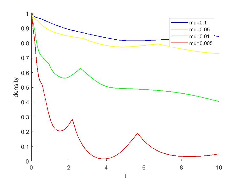
(a) Minimum of $\rho^{n+1}$

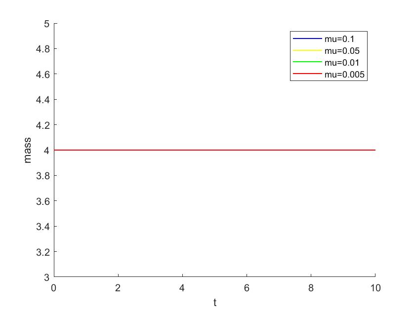
(b) Evolution of cell mass

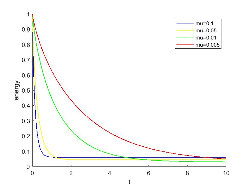
(c) Evolution of energy $E^{n+1}$

Figure 1: Evolutions of the density, mass and energy.

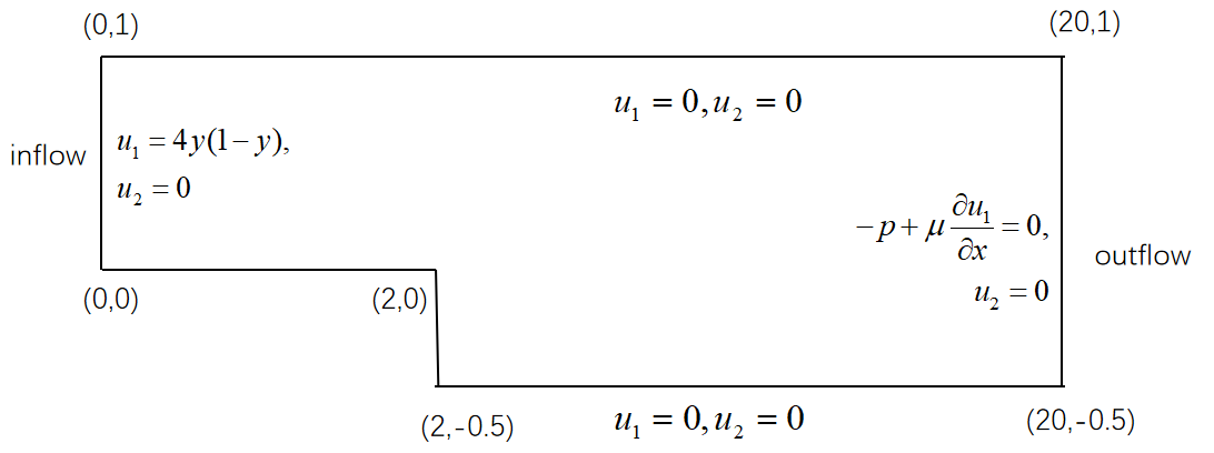
Figure 2: Analytical regions and boundary conditions.

Figure 3: Velocity $u_{1}$ of the back-step flow at $t=3$ (top), $t=5$ (middle), $t=7$ (bottom).

Figure 4: Velocity $u_{2}$ of the back-step flow at $t=3$ (top), $t=5$ (middle), $t=7$ (bottom).

Figure 5: Pressure $p$ of the back-step flow at $t=3$ (top), $t=5$ (middle), $t=7$ (bottom).

Figure 6: Velocity $u_{1}$ of the cylinder flow at $t=3$ (top), $t=5$ (middle), $t=7$ (bottom).

Figure 7: Velocity $u_{2}$ of the cylinder flow at $t=3$ (top), $t=5$ (middle), $t=7$ (bottom).

Figure 8: Pressure $p$ of the cylinder flow at $t=3$ (top), $t=5$ (middle), $t=7$ (bottom).