Inteval Analysis for two spherical functions arising from robust Perspective-n-Lines problem

Abstract

This report presents a comprehensive interval analysis of two spherical functions derived from the robust Perspective-n-Lines (PnL) problem. The study is motivated by the application of a dimension-reduction technique to achieve global solutions for the robust PnL problem. We establish rigorous theoretical results, supported by detailed proofs, and validate our findings through extensive numerical simulations.

1 Preliminary

Notations: we use the notation $\mathbf{a}\bullet\mathbf{b}\triangleq\mathbf{a}^{\top}\mathbf{b}$, and use the notation $(\mathbf{a},\mathbf{b})\triangleq\begin{bmatrix}\mathbf{a}\\ \mathbf{b}\end{bmatrix}$ for the concatenation of two vectors. We use the notation ${}^{\mathcal{F}}\mathbf{a}$ to highlight that $\mathbf{a}$ is observed in the reference frame ${\mathcal{F}}$. Specifically, we denote the normalized camera frame as ${\mathcal{C}}$, and denote the world frame as ${\mathcal{W}}$.

1.1 Parameterization of Lines

Consider a 2D line in the image which writes as follows in the pixel coordinate:

$$\begin{bmatrix}A&B&C\end{bmatrix}(u,v,1)=0.$$

where the coefficients can be easily determined with two pixels on the line. According to the following linear transformation:

$$(x,y,1)=\mathbf{K}^{-1}(u,v,1),$$

where $\mathbf{K}$ is the camera intrinsic matrix, we can write the same line in the normalized image coordinate as

$$\begin{bmatrix}A_{c}&B_{c}&C_{c}\end{bmatrix}(x,y,1)=0,$$

with $\begin{bmatrix}A_{c}&B_{c}&C_{c}\end{bmatrix}=\begin{bmatrix}A&B&C\end{bmatrix}\mathbf{K}$. We use the normalized coefficient vector $\vec{\mathbf{n}}$ to parameterize a 2D line $l_{c}$ in the normalized camera coordinate:

$${}^{\mathcal{C}}\vec{\mathbf{n}}=\frac{(A_{c},B_{c},C_{c})}{\|(A_{c},B_{c},C_{c})\|},~~l_{c}:=\{{}^{\mathcal{C}}\mathbf{p}\in\mathbb{R}^{2}|{}^{\mathcal{C}}\vec{\mathbf{n}}\bullet({}^{\mathcal{C}}\mathbf{p},1)=0\}.$$

We refer to ${}^{\mathcal{C}}\vec{\mathbf{n}}$ as the normal vector since it is perpendicular to the plane passing through the camera origin and $l_{c}$.

As for a 3D line $L_{w}$ observed in the world coordinate, we parameterize it with a point ${}^{\mathcal{W}}\mathbf{p}_{0}$ on it and a unit-length direction vector ${}^{\mathcal{W}}\vec{\mathbf{v}}$, such that

$$L_{w}:=\{{}^{\mathcal{W}}\mathbf{p}\in\mathbb{R}^{3}|({}^{\mathcal{W}}\mathbf{p}-{}^{\mathcal{W}}\mathbf{p}_{0})\times{}^{\mathcal{W}}\vec{\mathbf{v}}=0\}.$$

1.2 Projection Model

Assume the relative transformation from the normalized camera frame to the world coordinate writes as follows

$${}^{\mathcal{W}}_{\mathcal{C}}\mathbf{T}=\begin{bmatrix}\mathbf{R}&\mathbf{t}\\ \mathbf{0}^{\top}&1\end{bmatrix}.$$

Assume a 2D line $l_{c}$ with normal vector ${}^{\mathcal{C}}\vec{\mathbf{n}}$ is the projection of a 3D line $L_{w}$ parameterized with ${}^{\mathcal{W}}\vec{\mathbf{v}}$ and ${}^{\mathcal{W}}\mathbf{p}_{0}$, the following two equations Liu et al. (1990) uniquely determine the projection:

$${}^{\mathcal{C}}\vec{\mathbf{n}}\bullet\mathbf{R}^{\top}{}^{\mathcal{W}}\vec{\mathbf{v}} =0,$$ (1)

$$(\mathbf{R}{}^{\mathcal{C}}\vec{\mathbf{n}})\bullet({}^{\mathcal{W}}\mathbf{p}_{0}-\mathbf{t}) =0.$$ (2)

1.3 Accelerating Consensus Maximization

Consider the following 1d CM problem:

$$\max_{b\in\mathcal{X}}\sum_{k=1}^{K}\mathbf{1}\{|f(b|\mathbf{s}_{k})|\leq\epsilon\},$$ (3)

where $b$ is a scalar parameter that belongs to $\mathcal{X}\subseteq\mathbb{R}$, $\mathbf{s}_{k}$ is data, and $f(b|\mathbf{s}_{k})$ is the residual function continuous in $b$. Suppose we can obtain $|f(b|\mathbf{s}_{k})|\leq\epsilon\Leftrightarrow b\in\bigcup_{l}[b_{kl}^{l},b_{kl}^{r}]$, the authors of  Zhang et al. (2024) observe that problem (3) is equivalent to the following interval stabbing problem:

$$\max_{b\in\mathcal{X}}\sum_{k=1}^{K}\sum_{l}\mathbf{1}\{b\in[b_{kl}^{l},b_{kl}^{r}]\}.$$ (4)

Next, consider a n-d CM problem:

$$\max_{\mathbf{b}\in\mathcal{X}\subseteq\mathbb{R}^{n}}\sum_{k=1}^{K}\mathbf{1}\{|f(\mathbf{b}|\mathbf{s}_{k})|\leq\epsilon\}.$$ (5)

The ACM method distinguishes one parameter with others, $\mathbf{b}=(\mathbf{b}_{1:n-1},b_{n})$, and branches only the space of $\mathbf{b}_{1:n-1}$. This is achieved by revising the bound-seeking procedure. Suppose we are seeking bounds for $\mathbf{b}_{1:n-1}\in\boldsymbol{\mathcal{C}}_{1:n-1}$ and $b_{n}$.

1.3.1 Lower Bound

Denote the consensus maximizer as $(\mathbf{b}^{*}_{1:n-1},b_{n}^{*})$, ACM finds a lower bound as follows, $\sum_{k=1}^{K}\mathbf{1}\{|f(\mathbf{b}_{1:n-1}^{*},b_{n}^{*}|\mathbf{s}_{k})|\leq\epsilon\}$

$$\geq~\max_{b_{n}}\sum_{k=1}^{K}\mathbf{1}\{|f(b_{n}|\mathbf{b}_{1:n-1}^{(c)},\mathbf{s}_{k})|\leq\epsilon\},$$

where $\mathbf{b}_{1:n-1}^{(c)}$ is the center point of $\boldsymbol{\mathcal{C}}_{1:n-1}$. Notice that the lower bound corresponds to a 1-d CM problem, and it can be efficiently solved by interval stabbing as we do in (4).

1.3.2 Upper Bound

If a consensus problem can be written as

$$\max_{\mathbf{b}\in\mathcal{X}}\sum_{k=1}^{K}\mathbf{1}\{|\sum_{i}f_{i}(b_{n},h_{i}(\mathbf{b}_{1:n-1},\mathbf{s}_{k})|\mathbf{s}_{k})|\leq\epsilon\}$$ (6)

where $h_{i}(\mathbf{b}_{1:n-1})$ is a function of $\mathbf{b}_{1:n-1}$. And if all $f_{i}$ are monotonically increasing(it’s similar to decreaseing condition) in $h_{i}$, set that

$$h_{i}^{L}\leq h_{i}(\mathbf{b}_{1:n-1},\mathbf{s}_{k})\leq h_{i}^{U}$$ (7)

we can get

$$f_{L}(b_{n}|\mathbf{s}_{k})=\sum_{i}f_{i}(b_{n}|h_{i}^{L},\mathbf{s}_{k})\leq\sum_{i}f_{i}(b_{n},h_{i}(\mathbf{b}_{1:n-1},\mathbf{s}_{k})|\mathbf{s}_{k})\leq\sum_{i}f_{i}(b_{n}|h_{i}^{U},\mathbf{s}_{k})=f_{U}(b_{n}|\mathbf{s}_{k})$$ (8)

Given these bounding functions, ACM finds an upper bound as follows, $\sum_{k=1}^{K}\mathbf{1}\{|f(\mathbf{b}_{1:n-1}^{*},b_{n}^{*}|\mathbf{s}_{k})|\leq\epsilon\}$

$$\leq\max_{b_{n}}\sum_{k=1}^{K}\mathbf{1}\left[\{f_{L}(b_{n}|\mathbf{s}_{k})\leq\epsilon\}\bigcap\{f_{U}(b_{n}|\mathbf{s}_{k})\geq-\epsilon\}\right]$$ (9)

which can be solved by interval stabbing.

Readers can refer to Zhang et al. (2024)’s work for the detailed introduction and other applications of the accelerating consensus maximization algorithm.

2 Problem Formulation

2.1 Basic problem

Given a set of 3D lines $\{L_{w_{i}}\}_{i=1}^{N}$ and their corresponding 2D lines $\{l_{c_{i}}\}_{i=1}^{N}$, the CM problem for the PnL problem can be formulated as follows:

$$\mathop{\rm max}\limits_{\mathbf{R}\in SO(3)}~~\sum_{k}\boldsymbol{1}\{|\mathbf{}{}^{\mathcal{C}}\vec{\mathbf{n}}_{k}\bullet\mathbf{R}^{\top}{}^{\mathcal{W}}\vec{\mathbf{v}}_{k}|<=\epsilon_{r}\},$$ (10)

where $\vec{\mathbf{v}}_{k}$ represent the direction of 3D lines, $\vec{\mathbf{n}}_{k}$ represent the normalized coefficient vector of 2D lines.

2.2 How to accelerate?

In the rotation estimation problem (10), we parameterize rotation with a rotation axis $\vec{\mathbf{u}}\in\mathbb{S}^{3}$ and an amplitude $\theta\in[0,\pi]$. We choose $\theta$ as the distinguished parameter, and further parameterize $\vec{\mathbf{u}}$ by polar coordinates:

$$\vec{\mathbf{u}}=(\sin{\alpha}\cos{\phi},\sin{\alpha}\sin{\phi},\cos{\alpha})~~\alpha\in[0,\pi]~\phi\in[0,2\pi].$$

Denote data from a pair of 2D/3D line matching as $\mathbf{s}_{k}\triangleq(\vec{\mathbf{v}}_{k},\vec{\mathbf{n}}_{k})$, we can write the observation function for (10) as

$$\mathbf{}{}^{\mathcal{C}}\vec{\mathbf{n}}_{k}\bullet\mathbf{R}^{\top}{}^{\mathcal{W}}\vec{\mathbf{v}}_{k}=\vec{\mathbf{n}}_{k}^{\top}\vec{\mathbf{v}}_{k}+\sin{\theta}\vec{\mathbf{n}}_{k}^{\top}(\vec{\mathbf{u}}\times\vec{\mathbf{v}}_{k})+(1-\cos{\theta})\vec{\mathbf{n}}_{k}^{\top}[\vec{\mathbf{u}}]_{\times}^{2}\vec{\mathbf{v}}_{k},$$ (11)

Rearrange the terms in (11) likes (6), we can get

$$\begin{cases}f_{1}(\theta,h_{1}(\vec{\mathbf{u}},\mathbf{s}_{k}),s_{k})=\vec{\mathbf{n}}_{k}^{\top}\vec{\mathbf{v}}_{k}+\sin{\theta}h_{1}&\text{where }h_{1}(\vec{\mathbf{u}}|\mathbf{s}_{k})\triangleq\vec{\mathbf{u}}^{\top}(\vec{\mathbf{v}}_{k}\times\vec{\mathbf{n}}_{k})\\ f_{2}(\theta,h_{2}(\vec{\mathbf{u}},\mathbf{s}_{k}),s_{k})=(1-\cos\theta)h_{2}&\text{ where }h_{2}(\vec{\mathbf{u}}|\mathbf{s}_{k})\triangleq\vec{\mathbf{n}}_{k}^{\top}[\vec{\mathbf{u}}]_{\times}^{2}\vec{\mathbf{v}}_{k}\end{cases}$$ (12)

As long as we can find the lower and upper bounds for $h_{1}$ and $h_{2}$, we can find the accessible intervals for upper bound of (5) according to (9).

2.3 conclusions

For clarity, we denote the sub-cube as

$$\boldsymbol{\mathcal{C}}_{\vec{\mathbf{u}}}\triangleq\{(\alpha,\phi)|\alpha\in[\underline{\alpha},\bar{\alpha}],\phi\in[\underline{\phi},\bar{\phi}]\},$$

denote the boundary of $\boldsymbol{\mathcal{C}}_{\vec{\mathbf{u}}}$ as $\partial\boldsymbol{\mathcal{C}}_{\vec{\mathbf{u}}}$, and denote

$$\vec{\mathbf{m}}_{k}=\frac{\vec{\mathbf{v}}_{k}+\vec{\mathbf{n}}_{k}}{\|\vec{\mathbf{v}}_{k}+\vec{\mathbf{n}}_{k}\|},~~\vec{\mathbf{m}}_{k}^{\perp}=\frac{\vec{\mathbf{v}}_{k}-\vec{\mathbf{n}}_{k}}{\|\vec{\mathbf{v}}_{k}-\vec{\mathbf{n}}_{k}\|},~~\vec{\mathbf{c}}_{k}\triangleq\frac{\vec{\mathbf{v}}_{k}\times\vec{\mathbf{n}}_{k}}{\|\vec{\mathbf{v}}_{k}\times\vec{\mathbf{n}}_{k}\|}.$$

We summarize our results in the following theroems:

2.3.1 Theorem and proof of $h_{2}$

Theorem 1 (Extreme Point Theorem for $h_{2}(\vec{\mathbf{u}}|\mathbf{s}_{k})$).

1. If $\pm\vec{\mathbf{m}}_{k}\in\boldsymbol{\mathcal{C}}_{\vec{\mathbf{u}}}$, we have $\arg\max_{\vec{\mathbf{u}}}h_{2}(\vec{\mathbf{u}}|\mathbf{s}_{k})=\pm\vec{\mathbf{m}}_{k}.$

2. If $\pm\vec{\mathbf{m}}_{k}^{\perp}\in\boldsymbol{\mathcal{C}}_{\vec{\mathbf{u}}}$, we have $\arg\min_{\vec{\mathbf{u}}}h_{2}(\vec{\mathbf{u}}|\mathbf{s}_{k})=\pm\vec{\mathbf{m}}_{k}^{\perp}$.

   

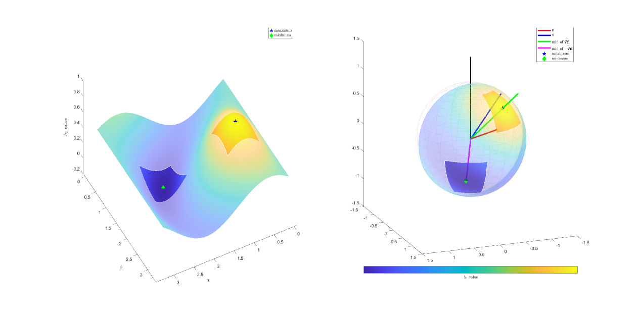
   Figure 1: Illustration of the first and second cases in Theorem 1.

3. Otherwise, the extreme points fall on $\partial\boldsymbol{\mathcal{C}}_{\vec{\mathbf{u}}}$.

   

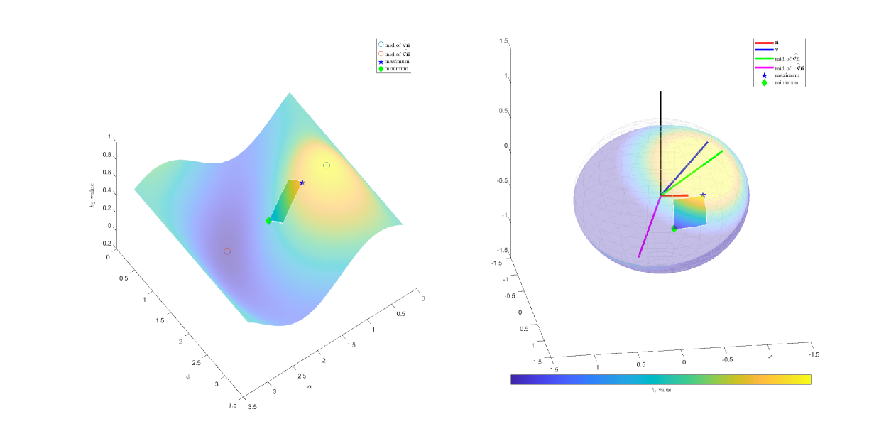
   Figure 2: Illustration of the third case in Theorem 1.

Proof.

TBD ∎

2.3.2 Theorem and proof of $h_{1}$

Theorem 2 (Extreme Point Theorem for $h_{1}(\vec{\mathbf{u}}|\mathbf{s}_{k})$).

1. If $\vec{\mathbf{c}}_{k}\in\boldsymbol{\mathcal{C}}_{\vec{\mathbf{u}}}$, we have $\arg\max_{\vec{\mathbf{u}}}h_{1}(\vec{\mathbf{u}}|\mathbf{s}_{k})=\vec{\mathbf{c}}_{k}.$

2. If $-\vec{\mathbf{c}}_{k}\in\boldsymbol{\mathcal{C}}_{\vec{\mathbf{u}}}$, we have $\arg\min_{\vec{\mathbf{u}}}h_{1}(\vec{\mathbf{u}}|\mathbf{s}_{k})=-\vec{\mathbf{c}}_{k}$.

   

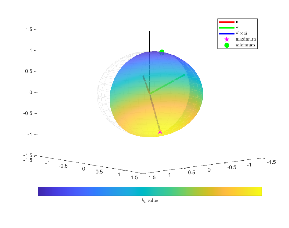
   Figure 3: Illustration of the first and second cases in Theorem 2.

3. Otherwise, the extreme points fall on $\partial\boldsymbol{\mathcal{C}}_{\vec{\mathbf{u}}}$.

   

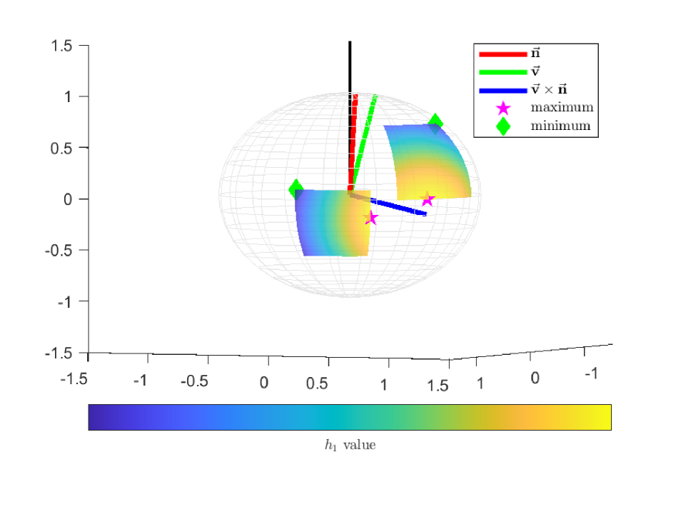
   Figure 4: Illustration of the third case in Theorem 2.

The proof for Theorem 2 is similar to and easier than the proof for Theorem 1, thus we omit the proof here and focus on discussing the third case in Theorem 2. Denote the polar coordinates for $\vec{\mathbf{c}}_{k}$ as $(\alpha_{k},\phi_{k})$, we have:

$$h_{1}(\vec{\mathbf{u}}|\mathbf{s}_{k})\propto(\sin{\alpha_{k}}\sin{\alpha}\cos{(\phi_{k}-\phi)}+\cos{\alpha_{k}}\cos{\alpha}),$$ (13)

where the constant term $\|\vec{\mathbf{v}}_{k}\times\vec{\mathbf{n}}_{k}\|$ is omitted. The partial derivative of $h_{1}$ with respect to $\alpha$ and $\phi$ writes

$$\frac{\partial h_{1}}{\partial\alpha} \propto\sin{\alpha_{k}}\cos{\alpha}\cos{(\phi_{k}-\phi)}-\sin{\alpha}\cos{\alpha_{k}},$$ (14a)

$$\frac{\partial h_{1}}{\partial\phi} \propto\sin{\alpha_{k}}\sin{\alpha}\sin{(\phi_{k}-\phi)}.$$ (14b)

Without loss of generality, we only consider the case where both the sub-cube $\boldsymbol{\mathcal{C}}_{\vec{\mathbf{u}}}$ and $\vec{\mathbf{c}}_{k}$ belong to the east-hemisphere, i.e., $\phi_{k}\in[0,\pi]$ and $\phi\in[0,\pi]$. Denote polar coordinates which minimize $h_{1}$ as $\alpha_{\rm min}$ and $\phi_{\rm min}$ respectively, and denote the maximizers as $\alpha_{\rm max}$ and $\phi_{\rm max}$ respectively. Use notations $\alpha_{\rm near}$ and $\phi_{\rm near}$ as

$$\alpha_{\rm near}\triangleq\mathop{\arg\min}_{\alpha\in[\alpha_{l},\alpha_{r}]}|\alpha-\alpha_{k}|,~~\phi_{\rm near}\triangleq\mathop{\arg\min}_{\phi\in[\phi_{l},\phi_{r}]}|\phi-\phi_{k}|.$$

Note that $\alpha_{\rm near}=\alpha_{k}$ if $\alpha_{k}\in[\alpha_{l},\alpha_{r}]$. Similarly, we use notations $\alpha_{\rm far}$ and $\phi_{\rm far}$. We first give a lemma for $\phi$:

Lemma 1.

If $(\alpha,\phi)\in\partial\boldsymbol{\mathcal{C}}_{\vec{\mathbf{u}}}$ is a extreme point for $h_{1}(\vec{\mathbf{u}}|\mathbf{s}_{k})$ on the boundaries of cube, one must have

$$\phi_{\rm max}=\phi_{\rm near},\phi_{\rm min}=\phi_{\rm far}.$$

Proof.

Based on the partial derivative (14b), we highlight two observations. (1) For a fixed $\alpha\in[0,\pi]$, we have $\frac{\partial h_{1}}{\partial\phi}>0$ if $\phi<\phi_{k}$, and $\frac{\partial h_{1}}{\partial\phi}<0$ if $\phi>\phi_{k}$. (2) The partial derivative takes the same value for $\phi_{1}$ and $\phi_{2}$ equally close to $\phi_{k}$. Based on the above two observations, we naturally conclude this lemma. ∎

After we fix $\phi$ at either $\phi_{\rm near}$ or $\phi_{\rm far}$, we focus on the partial derivative  (14a).

Lemma 2.

For $\alpha_{k}\not=\pi/2$, the partial derivative  (14a). has a unique zero point $\alpha^{*}\in[0,\pi]$. For a fixed $\phi$, the zero point $\alpha^{*}$ is a global maximizer if $|\phi_{k}-\phi|<\pi/2$, and is a global minimizer if $|\phi_{k}-\phi|<\pi/2$.

Proof.

The partial derivative (14a) can be organized in the form of $A\sin{(\alpha+\bar{\beta})}$, with $\bar{\beta}$ as fixed angle. For $\alpha_{k}\not=\pi/2$, we have $\bar{\beta}\not=0$, and as a result there exist a unique zero point $\alpha^{*}\in[0,\pi]$. If $|\phi_{k}-\phi|\not=\pi/2$ and $\alpha\not=\pi/2$, we can rewrite (14a) as:

$$\frac{\partial h_{1}}{\partial\alpha}=cos{\alpha_{k}}cos{\alpha}(\tan{\alpha_{k}}\cos{(\phi_{k}-\phi)}-\tan{\alpha}).$$ (15)

We discuss four cases in the table below, and the results are easy to verify using (15). From the table, we can observe that $\cos\alpha_{k}\cos\alpha^{*}>0$ for $\Delta\phi<\pi/2$, and $\cos\alpha_{k}\cos\alpha^{*}<0$ for $\Delta\phi>\pi/2$. We naturally arrive at the conclusion in this lemma based on this observation.

Table 1: Four different cases of $\alpha_{k}$ and $\Delta\phi$

$\alpha_{k}$	$\Delta\phi$	$\alpha^{*}\in$	$\cos\alpha_{k}\cos\alpha^{*}$
$<\pi/2$	$<\pi/2$	$(0,\alpha_{k})$	$>0$
$>\pi/2$	$<\pi/2$	$(\alpha_{k},\pi)$	$>0$
$<\pi/2$	$>\pi/2$	$(\pi-\alpha_{k},\pi)$	$<0$
$>\pi/2$	$>\pi/2$	$(0,\pi-\alpha_{k})$	$<0$

∎

Remark 1.

Notice that we omit to discuss the special cases where $\alpha_{k}=\pi/2$ or $|\phi-\phi_{k}|=\pi/2$ for the sake of simplicity. These special cases are easy to handle, interested readers can refer to our code for details.

Combining Lemma 2 and Lemma 1, we propose a efficient procedure to find extreme points of $h_{1}(\vec{\mathbf{u}}|\mathbf{s}_{k})$ on $\partial\boldsymbol{\mathcal{C}}_{\vec{\mathbf{u}}}$. First of all, we find the maximizer with $\phi=\phi_{\rm near}$. Denote $\Delta\phi_{\rm near}\triangleq|\phi_{k}-\phi_{\rm near}|$.

1. If $\Delta\phi_{\rm near}=0$, we have

   $$\alpha_{\rm max}=\alpha_{\rm near}.$$

2. if $\Delta\phi_{\rm near}=\pi/2$

   $$\alpha_{\max}=\begin{cases}\alpha_{1}&\text{if}\quad\alpha\leq\pi/2\\ \alpha_{2}&\text{if}\quad\alpha>\pi/2\par\end{cases}$$

3. If $\Delta\phi_{\rm near}>\pi/2$, we have

   $$\alpha_{\rm max}=\mathop{\arg\max}_{\alpha\in[\alpha_{l},\alpha_{r}]}|\alpha-\alpha^{*}(\Delta\phi_{\rm near})|.$$

4. If $\Delta\phi_{\rm near}<\pi/2$, $\alpha_{k}<\pi/2$, and $\alpha_{l}>=\alpha_{k}$, we have

   $$\alpha_{\rm max}=\alpha_{l}.$$

5. $\Delta\phi_{\rm near}<\pi/2$, $\alpha_{k}>\pi/2$, and $\alpha_{r}<=\pi-\alpha_{k}$, we have

   $$\alpha_{\rm max}=\alpha_{r}.$$

6. Otherwise, calculate $\alpha^{*}(\Delta\phi_{\rm near})$ and we have

   $$\alpha_{\rm max}=\mathop{\arg\min}_{\alpha\in[\alpha_{l},\alpha_{r}]}|\alpha-\alpha^{*}(\Delta\phi_{\rm near})|.$$

We can find the minimizer with $\phi=\phi_{\rm far}$ with a quite symmetrical procedure. Denote $\Delta\phi_{\rm far}=|\phi_{k}-\phi_{\rm far}|$.

1. If $\Delta\phi_{\rm far}<\pi/2$, we have

   $$\alpha_{\rm min}=\mathop{\arg\min}_{\alpha\in[\alpha_{l},\alpha_{r}]}|\alpha-\alpha^{*}(\Delta\phi_{\rm far})|.$$

2. if $\Delta\phi_{\rm near}=\pi/2$

   $$\alpha_{\min}=\begin{cases}\alpha_{2}&\text{if}\quad\alpha\leq\pi/2\\ \alpha_{1}&\text{if}\quad\alpha>\pi/2\par\end{cases}$$

3. If $\Delta\phi_{\rm far}>\pi/2$, $\alpha_{k}<\pi/2$, and $\alpha_{r}<=\pi-\alpha_{k}$, we have

   $$\alpha_{\rm min}=\alpha_{r}.$$

4. $\Delta\phi_{\rm far}>\pi/2$, $\alpha_{k}>\pi/2$, and $\alpha_{l}>=\pi-\alpha_{k}$, we have

   $$\alpha_{\rm min}=\alpha_{l}.$$

5. Otherwise, calculate $\alpha^{*}(\Delta\phi_{\rm far})$ and we have

   $$\alpha_{\rm min}=\mathop{\arg\min}_{\alpha\in[\alpha_{l},\alpha_{r}]}|\alpha-\alpha^{*}(\Delta\phi_{\rm far})|.$$

References

- Liu et al. [1990] Y. Liu, T. S. Huang, and O. D. Faugeras. Determination of camera location from 2-d to 3-d line and point correspondences. IEEE Transactions on pattern analysis and machine intelligence, 12(1):28–37, 1990.
- Zhang et al. [2024] X. Zhang, L. Peng, W. Xu, and L. Kneip. Accelerating globally optimal consensus maximization in geometric vision. IEEE Transactions on Pattern Analysis and Machine Intelligence, 2024.