1.5
Kyushu University Working Paper \pubMonthMAR \pubYear2025 \pubVolumeVol \pubIssueIssue \JEL \Keywords
The Evolution of Health Investment: Historical Motivations and Fertility Implications
Abstract
In this working paper, I developed a suite of macroeconomic models that shed light on the intricate relationship between economic development, health, and fertility. These innovative models conceptualize health as an intermediate good, paving the way for new interpretations of dynamic socio-economic phenomena, particularly the non-monotonic effects of health on economic and population growth. The evolving dynamic interactions among economic growth, population, and health during the early stages of human development have been well interpreted in this research.
1 Introduction
Although a large body of literature provides empirical evidence on the impact of health improvements on economic growth, the mechanism through which health investment interacts with economic development and population growth remains ambiguous. More importantly, the differences between developing and developed countries in our empirical results suggest that health plays different roles at different stages of development. That is, it is reasonable to assume that health investment strategies have been evolving over time.
In fact, empirical evidence(Acemoglu, Robinson &Johnson, 2003; Fogel, 2004; Galor, 2005; Weil, 2005; Finlay, 2007; Cutler, Lleras-Muney & Vogl, 2012 ; Szreter, 2021; Missoni, 2023 ) does indicate that health investment decisions have evolved significantly over different historical periods, shaped by diverse economic, social, and technological factors. Specifically, much research has indicated (Fogel, 1994; Weil, 2007; Bloom & Canning, 2008) that better health contributes to higher labor productivity and economic growth in the modern economy. Apart from that, Fisher’s earlier study (1909) was the first to emphasize health as a form of wealth, advocating for investments in public health to enhance national economic productivity. This perspective laid the groundwork for considering health from an economic standpoint in the early 20th century. From a demographic perspective, Becker (1960) argued that health improvements, particularly lower infant mortality rates, could lead to demographic transitions, shifting societies from high birth rates to lower, more sustainable population growth rates. Grossman (1972) then introduced the health capital model, conceptualizing health as a durable capital good that individuals invest in to increase both utility and productivity. Grossman’s model posited that individuals make decisions about health investments by balancing the costs of medical care and healthy behaviors against the benefits of improved health and longevity. Soares (2005) proposed a model emphasizing that reductions in mortality serve as a driving factor for economic development. This model replicates patterns resembling the demographic transition, where an increase in life expectancy at birth is accompanied by declining fertility rates and accelerated human capital accumulation. This transition begins when life expectancy at birth reaches a critical threshold, signaling the economy’s shift from a Malthusian equilibrium to a state characterized by human capital investments and the potential for sustained long-term growth.
As Fogel (1994) well summarized, the role of health investments in driving productivity improvements is clear during industrialization and beyond. However, this explanation does not always hold historically. For example, current theories struggle to explain Clark (2007)’s empirical findings, which suggested the very early agricultural sector, despite its initial negative impacts on health outcomes due to poorer nutrition and higher (infectious) disease rates, managed to achieve overall production development and population expansion. An interesting counterpart during the Middle Ages was that, particularly in Western Europe, public health investment decisions were strongly shaped by religious doctrines and the prevailing humoral theory (McVaugh, 1993; Biller, 2001; Brunton, 2004; Elmer, 2004).
The evolution of health investment decisions highlights a growing recognition of health as a critical economic asset. From early theoretical frameworks to modern empirical studies, the interplay between health, population, and economic development has become increasingly apparent, emphasizing the importance of strategic health investments in fostering economic growth and enhancing societal well-being.
While it is evident that the role of health in economic development has evolved throughout history, debates persist — particularly regarding its role in ancient economies, which remains ambiguous. Some counterintuitive evidence, such as that presented by Clark (2007), continues to lack a robust theoretical explanation. In the following sections of this chapter, we will begin by addressing this specific issue and then interpret the evolving roles that health played in early human societies.
2 First Stage Model
The advent of early agriculture marked a significant transition from hunter-gatherer societies to settled agricultural communities, profoundly influencing human health. However, this transition also introduced complex health challenges. Cohen (1989) highlighted a notable decline in overall health among early agricultural populations compared to hunter-gatherers. This decline was evident in the increased prevalence of skeletal and dental pathologies, as well as altered growth patterns. Bocquet-Appel (2002) explored the relationship between population growth and declining health during the rise of agriculture. The study revealed that sedentism and agricultural intensification led to the spread of infectious diseases and nutritional deficiencies, particularly among infants and children. In addition, Larsen (2014) examined the global health implications of the transition from foraging to farming. Using archaeological evidence, Larsen demonstrated how this transition altered disease patterns and worsened nutritional outcomes, significantly impacting human health and lifestyle. As an article by ScienceDaily (2011) summarized, early agriculture led to widespread nutritional deficiencies and reduced adaptability to stress. These challenges were primarily attributed to dependence on specific crops and higher population densities.
In other words, the archaeological evidence indicates that early agricultural technologies actually reduced human health levels. However, the population within the agricultural sector continued to grow and eventually replaced hunting and gathering. The decline in health during early agriculture is well explained — whether due to the spread of infectious diseases from domesticated animals or less diverse diets compared to those of the hunting-gathering sector, both factors contributed to poorer health. In contrast, the population growth within the agricultural sector appears counterintuitive. This phenomenon will be examined and explained using the following model.
In the first stage model below, we assume the existence of an intermediate health production. People can invest in this production to achieve better health levels, which in turn reduces their investment in the regular production sector. This setting represents a very ancient stage of human, when agriculture was only recently and accidentally invented.
Consider an ancient overlapping generations economy in which economic activity extends to infinite discrete time. In every period , this ancient economy produces the final good using labor and land. The land supply is exogenous and constant (because limited productivity prevents additional land from generating extra output). Labor is allocated between intermediate health production (i.e., investment in health) and physical production that are directly associated with the final good. Households supply their labor inelastically and the population grows at the endogenously determined rate. The intermediate production resulting from one’s health investment is defined as:
where is a parameter, is the labor (fraction) that allocated to intermediate health production (e.g., opportunity cost, labor related to health improvement or time spent on health-increasing activities) and is the total labor supply at time . So the fraction of pure physical labor is .
The per capita intermediate health production is defined as:
In other words, the representative household is endowed with level intermediate health technology, where is productivity of the health intermediate good at time .
2.1 The Aggregate Production of Final Output
In the early stages of human civilization, the natural environment posed significant challenges to human health, lifespan, and productivity. When ancient people faced various health-related threats, balancing physical well-being and working hours became crucial. They had many ways to improve their health, with the most direct and effective being to rest more and free themselves from heavy physical labor. Additionally, building safer shelters to reduce the risks posed by harsh weather and dangerous animals was another key strategy. Thus, we assume that one of the motivations for our ancestors to improve their health stemmed from their health-related environment or environmental adversity.
The aggregate production function is given by:
where denotes the level of environmental adversity and is land supply. Noticeably, the impact of health intermediate technology per physical working labor can be abated by environmental adversity in the final production. So the first term in the aggregate production function, , can be also defined as the relative health technology.
Given that an ancient economy is modeled, the assumption of no return to land holds, as explained by Ricardo (1817)’s theory. That is, is normalized to 1. Thus, output per capita at time is
and assuming to guarantee positive output.
2.2 Labor Allocation
Households decide how to allocate their labor (or working time) between intermediate health production and final physical production at time , , in order to maximize final output under the environmental fluctuation, . The problem of labor allocation at time is defined as:
subject to
Solving the above problem suggests that the optimal allocation of labor depends on environmental adversity and the productivity of intermediate health goods. With the optimal allocation, we have:
Lemma 3.1 The optimal labor allocation is a monotonically increasing function of environmental adversity. That is, a worsening health environment induces households to allocate a larger fraction of their labor to intermediate health production sector.
The first lemma shows that one of the motivations for ancient humans to improve their health or increase health investments was to counter environmental risks. When they faced greater environmental fluctuations, they became more concerned about their health. One plausible intuition is that, in the absence of these risks, they did not need to make additional efforts to improve their health and could continue or maintain their production and lifestyle patterns as usual in this productivity-limited economy.
Similarly, we define the optimal level of output as a function of the health productivity, , the environmental adversity, , and the total labor supply, :
Solving the production maximization problem and the first and second-order partial derivatives of (3.7) suggest:
Lemma 3.2 Higher productivity of health intermediate goods promotes an individual’s output; a better health-related environment increases the average output; while a larger supply of labor will decrease the average output due to the fixed supply
of land.
The above derivation results also suggest a decelerating negative effect of total labor supply on household income.
2.3 Childbirth Preference
We assume the representative individual has a single parent and lives for two time periods, and . At time , the parent takes care of the individual until the individual joins the labor force at time . The parent needs to spend a fraction of his or her output to raise the children. That is, the generation is supposed to optimally allocate their income between consumption and raising children.
The representative utility function in the first stage is
where is the consumption of an individual at time ; is the number of children; is the preference of having children; and is the preference of consumption.
Also, the budget constraint for the representative individual is
Before moving to the utility optimization problem, we need to introduce another important assumption for this ancient economy: there exists a minimum level of consumption for the individual to survive, . This implies that another implicit constraint
which suggests that the optimal level of childbirth should ensure the individual’s survival.
Therefore, the utility optimization problem is set as:
subject to and
Another intuitive assumption is that, given the low level of productivity for the representative household at this very early stage of human history, the survival consumption constraint must be binding. The individual consumes at the minimum level , and uses the rest of his or her income for rearing children. We denote as the surviving level of income at which the surviving constraint is binding. Now we can derive the optimal level of childbirth for two different scenarios:
For this first-stage ancient period, we always assume only the second scenario applies:
In other words, the optimal level of childbirth is
Therefore, the propositions of the optimal level number of children follow trivially the previous lemmas of and is increasing in . We will revisit this part later in the context of the dynamics of health productivity in the following sections.
2.4 The Dynamic of Health Productivity
As this model represents an ancient economy, it is natural to consider that an individual’s motivation to improve health productivity is not constant, as they must also address many other survival-related challenges directly. Due to limited resources, survival takes precedence over achieving better health. However, introducing the environmental variable allows us to better describe their motivations. When facing greater survival pressures or worse health environments, they will realize the necessity to improve their health productivity to enhance their overall health levels or production. On the other hand, when our ancestors faced a stable or even better health environment, they were not conscious of improving their health productivity.
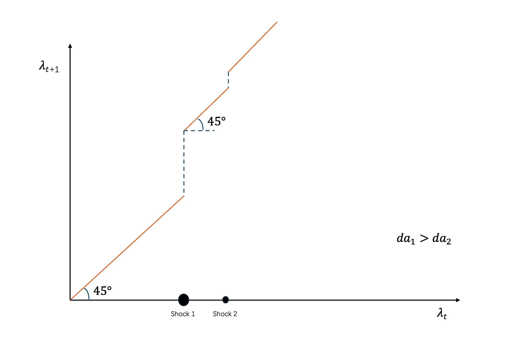
Based on this intuition, we can propose a dynamic for health productivity, . Thus, the law of motion for the productivity of the health intermediate good is given by:
where Function is strictly positive, increasing, and concave in the difference in the health investment between the generations. If generation ’s social health condition was worse than generation , thus , then generation ’s intermediate productivity will be benefited from this negative health shock. Otherwise, there is no motive or source for individuals to promote their health productivity.
This dynamic illustrates a well-documented historical phenomenon: improvements in health (productivity) are time-fragmented and permanent. That is, increases randomly whenever an environmental shock occurs (where the current environment is worse than the previous one).
2.5 Population Dynamic
Another historically consistent assumption is that all households die at the end of the first period. In other words, households in the second period are actually the offspring of those from the first period. Thus, the population’s law of motion is
Recall that (3.15) indicates that the optimal number of children, , is a strictly increasing function of the optimal income, , at time .
Thus, solving the production maximization problem suggests that the optimal number of children depends on health productivity , environmental adversity and total labor supply . With this , we can determine whether the population in the next period is increasing or decreasing.
Alternatively, there exists a population threshold for determining the sign of population change:
when , the population change is negative, and thus . Conversely, when , he population change is positive, resulting in .
Lemma 3.3 When the current population exceeds a certain threshold (determined as a function of and ), the fertility rate is less than 1, causing the population to decrease in the next period. Conversely, when the current population is below this threshold, the fertility rate is greater than 1, leading to population growth in the next period.
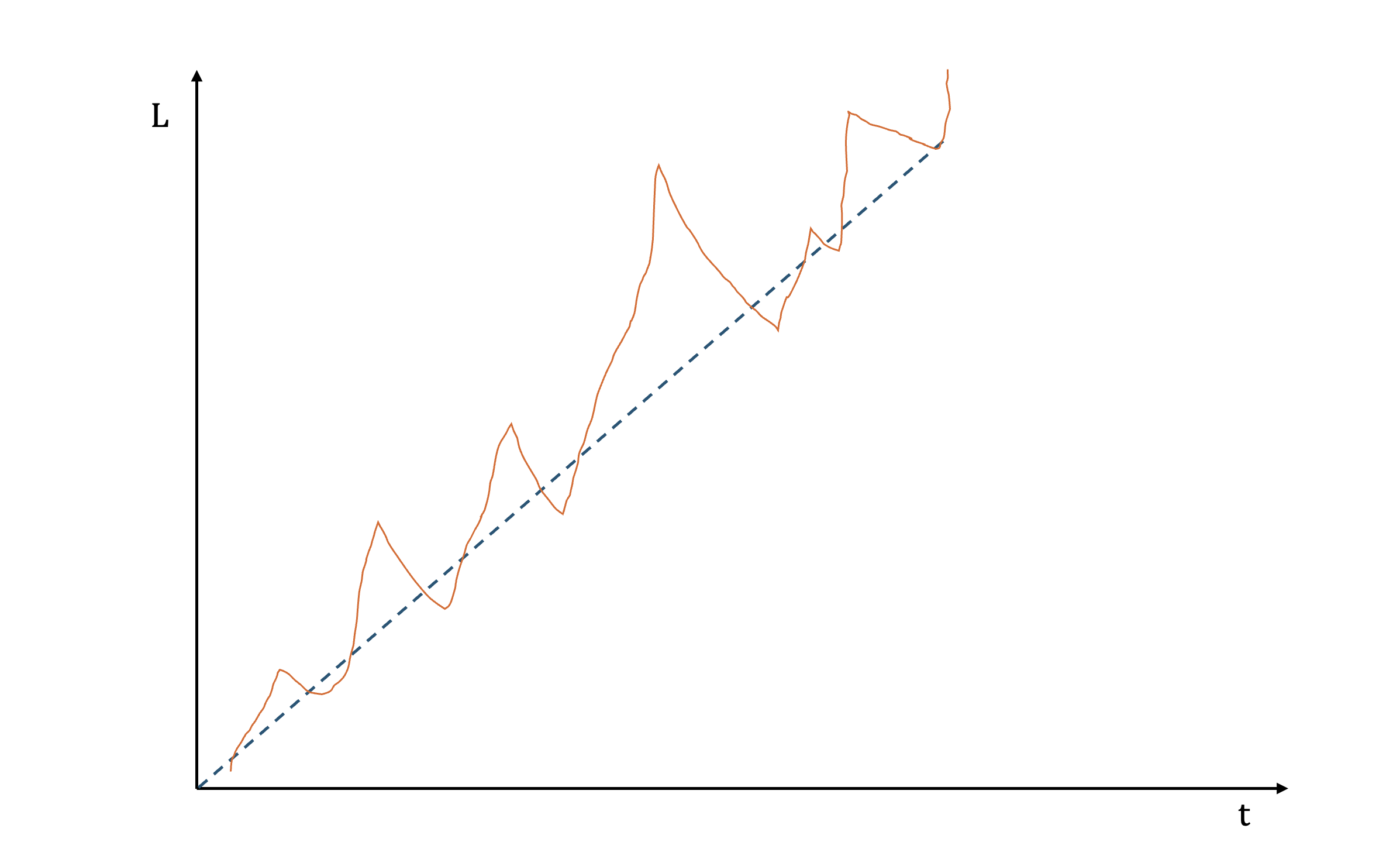
Although environmental shocks are random, we assume that in the very long run, the overall expected state of the environment is predictable to some extent. Then, using Lemmas , , and , we can preliminarily outline the population evolution path under two specific scenarios during this stage. The first scenario is that, when consistently holds during a certain period, we always have , and converges to 1 under the influence of random negative shocks. Under this first scenario, the population consistently decreases; however, the fertility rate gradually recovers to 1. On the other hand, the second scenario suggests that, when consistently holds during a certain period, the population growth rate decreases at first due to a negative shock, but we still have , or a positive population change. Under this second scenario, the population consistently increases. However, as the population size increases, this threshold condition cannot be sustained indefinitely. Eventually, the population size will adjust to the threshold value, at which it remains constant without the shock.
A more realistic scenario, considering population dynamics and random environmental shocks, is that Scenario 1 and Scenario 2 alternate frequently. In other words, whether environmental deterioration leads to a population decline depends on current health productivity and population size. When the population exceeds the capacity supported by environmental and productivity endowments, it will begin to decrease. In contrast, we observe a population increase when environmental and productivity endowments can afford a larger population. Since improvements in health productivity are irreversible, the population grows in the long run.
Proposition 3.1 In this initial stage, the evolution of health investment is essentially driven by negative environmental shocks, prompting people to increase health investment or productivity to ensure survival. In response to these shocks, health productivity undergoes an irreversible rise, resulting in higher output and fertility rate in subsequent periods.
Proposition 3.2 In this stage, the population follows an upward oscillatory trajectory, with increasing health productivity shaped by negative environmental shocks.
In summary, given the limited productivity in early human societies, people tended to adjust their fertility choices to closely align with environmental endowment. This explains why, despite long-term population growth driven by (health) productivity improvements, the short-term population change rate consistently tended to converge toward zero.
2.6 Implications of the First-Stage Model
This result strongly supports the historical phenomenon we previously mentioned: in early human history, the agricultural sector somehow degraded the environment, which was detrimental to health, yet it led to overall population growth. Specifically, corresponds to the first stage model, our ancestors accidentally adopted the agricultural technology (or production), and empirical evidence shows that this early agriculture indeed hurt human health (due to a less varied diet, diseases from domesticated animals, and reduced physical activity); nevertheless, the population continued to grow. This effectively explains the phenomenon where a poorer environment drives higher health productivity and increased population size.
3 Second Stage Model
With the development of (both health and physical) productivity and economy, the assumptions of the first-stage model cannot hold indefinitely, and the impact of environmental fluctuations on production and daily life will gradually diminish. In the next stage, both physical productivity and health productivity are assumed to increase to a new level, rendering the impact of the environment on production negligible. In other words, households no longer have an incentive to improve their health productivity, or, is normalized to 1.
So we set a new Cobb-Douglas production function for this second stage:
where and we still assume for this ancient economy. The per capita production is
In the initial stage, health investment was driven solely by the need for survival. However, with the advancement of society, we assume that in the second stage, households can also derive utility from health directly. Thus, the utility function for second-stage households is
In this second stage, the survival level of consumption is fully satisfied, so the budget constraint becomes
Then, solving the utility maximization problem subject to the above constraint yields:
substituting it into the constraint, we obtain the optimal level of childbirth:
And the optimal level of health investment is
The above results indicate that in this second stage, health investment depends solely on preferences for health and other parameters. This outcome is based on the assumption of a relatively stable environment compared to health productivity. Consequently, if preferences for health consumption remain unchanged, health investment during this stage remains constant.
3.1 Population Dynamic
We define the child mortality rate as an exogenous, environment-related variable beyond parental control and incorporate it into the population dynamics at this stage, where . Thus, the real population growth rate is
rewriting it, we have the following law of motion for the population
We define as the population level at which the fertility rate equals the child mortality:
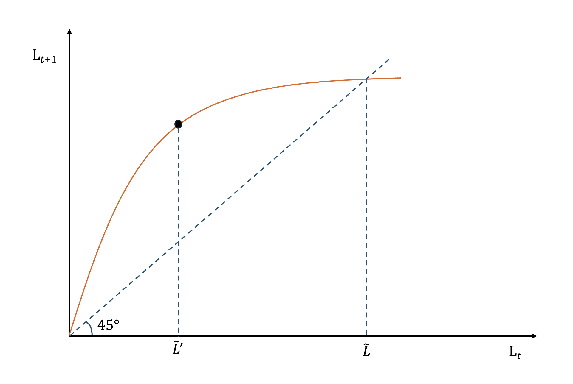
In this second stage, it is evident that the actual population growth rate is a decreasing function of the current population. More specifically, the following lemma applies:
Lemma 3.4 There exists a such that , where the population reaches its steady-state; there exists a such that we have the maximum level of , at which the population growth rate is maximized.
In this model, the child mortality rate can still be considered an increasing function of environmental adversity. The difference from the first-stage model lies in the assumption that the direct impact of the environment on production becomes negligible, affecting only population dynamics directly. In this case, can be replaced by for better consistency.
Proposition 3.3 In the second stage, if there is a negative environmental shock at time , the steady-state level of population decreases, the steady-state level of birth rate increases, and the steady-state level of consumption increases; if there is a positive environmental shock at time , the steady-state level of population increases, the steady-state level of birth rate decreases, and the steady-state level of consumption decreases.
In this thesis, we limit our exploration to the relatively short-term second stage, with a preliminary investigation of the subsequent third stage provided in the appendix. During this second stage, humanity underwent a relatively stable period of development. Population size fluctuated in response to changes in the natural environment but consistently converged to the steady state determined by its productivity endowments.
3.2 Implications
During this certain stage, productivity was sufficient to mitigate the environmental impact on household production, with the environment influencing households primarily through their offspring’s exogenous mortality.
Due to regional variations in environmental endowments, different areas exhibited different steady-state populations during this period. In other words, regions with more favorable environments tended to sustain larger populations. Compared to the previous historical period, health investment became stable or even constant. While the unpredictable natural environment continued to affect infant mortality, increased health investment had a negligible impact on adult productivity.
4 Conclusion
This chapter explores the role of health investment across different periods of human history by developing two macroeconomic models. Specifically, the first stage model provides an effective mechanism to explain the dynamic relationship between health investment, population, and production during the transition from hunting-gathering to agriculture in early human history. This model offers a compelling explanation for a counterintuitive historical phenomenon: while early agriculture adversely affects health level, the agricultural sector ultimately replaced the hunting-gathering sector.
As an extension to the next historical period, the second stage model provides a detailed depiction of the role health played in economic development and demographic dynamics during the later period, when agricultural technology had advanced and was no longer harmful. A more stable population size is revealed in this economy.
These two models show that the mechanisms by which health operates on economic development vary across historical periods. That is, the roles of health investment are evolving over time.
Clearly, we will continue to extend our model. However, before proceeding, it is important to emphasize that the two macroeconomic models presented in this thesis effectively demonstrate that health, as a critical economic factor, adopts different assumptions and functional roles across various historical periods and conditions. Specifically, in the models, health can be incorporated into production functions, utility functions, or even budget constraints with diverse forms, depending on the physical realities of each historical context.
5 Appendix
Proof of Lemma 3.1. The first-order condition of (3.5) yileds
The second-order condition yields
Similarly,
then apply the implicit function theorem and the proof is completed.
Proof of Lemma 3.2. FOC of yields
then we have the 2nd order partials:
then the proof is completed.
Derivation of Threshold .
Solve for the optimal level of , and set it equal to 1, then the derivation is completed.
Further Discussion: A Preliminary Experimental Model
In our first model, we assumed that early humans prioritized maximizing their income (the optimal production) for survival. However, in the subsequent historical period, survival is no longer a concern for the representative household. While capital accumulation is still absent, optimizing the household’s utility becomes the primary strategy during this stage. In the third stage, we maintain these assumptions but introduce a different consumption behavior in the utility function.
With further improvements in productivity, people’s consumption is no longer restricted to survival-related items. Consequently, we assume that healthier individuals derive greater utility from each unit of consumption.
In this scenario, we consider some multiplier effects of health investment on consumption utility in a revised preference framework:
subject to
where .
Instead of the previous constant cost of having children, we again assume a proportional term (the structure of this constraint is the same as in the first model, but the household adopts a different strategy).
Set the Lagrangian for above problem:
FOC:
Thus:
combine the first 2 equations in (3.32), we have:
This implies healthier households will have fewer children, primarily because they can derive greater utility from consumption with healthier physical conditions. Then we rewrite the 3rd equation in (3.32):
In the previous FOC, is a complex term to derive the result if we take the previous form of production function. Instead, we assume a compact production function (which still well represents the potential allocation between the health and physical sectors):
thus
and
Trivially, when , .
Rewrite (3.34):
so we have:
and for , we have
Lemma A3.1 There exists a certain interval of and , where we always have ; there exists a certain interval of and , where we always have ; the sign of depends on the ratio of to .
Implications: At this stage, the optimal level of health investment increases with both the productivity of physical labor and the preference for having children. Overall, the motivation for additional health investment at this stage stems from rising fertility preferences and increased labor productivity.
Historical evidence also supports the idea that, after human productivity surpassed survival levels and health conditions stabilized, our ancestors continued to invest in their health even in the absence of negative environmental challenges. On one hand, increased labor productivity encouraged individuals to maintain better health to secure corresponding income. On the other hand, higher fertility preferences motivated people to enhance their health to support their reproductive goals.
6 References
Acemoglu, D. and Johnson, S. (2007). “Disease and Development: The Effect of Life Expectancy on Economic Growth.” Journal of Political Economy, Vol. 115, No. 6, pp. 925–985.
Acemoglu, D. and Johnson, S. (2014). “A Reply to Bloom, Canning, and Fink.” Journal of Political Economy, Vol. 122, No. 6, pp. 1367–1375.
Aghion, P., Algan, Y., and Cahuc, P. (2009). “Can Policy Interact with Culture? Minimum Wage and the Quality of Labor Relations.” IZA Discussion Papers 3680, Institute of Labor Economics (IZA).
Radhakrishna, D and Ramachandra, N.U. “An Analysis of the Dowry System in India: Causes and Remedies.” (2021). Journal of Emerging Technologies and Innovative Research, Vol. 8, No. 6, pp. 151–156.
Bao, X., Bo, S., and Zhang, X. (2015). “Women as Insurance Assets in Traditional Societies,” retrieved from CUHK Economics Department Website.
Barro, R. J. (1996). Determinants of Economic Growth: A Cross-Country Empirical Study. Lionel Robbins Lectures.
Barzel, Y. (1969). “Productivity and the Price of Medical Services.” Journal of Political Economy, Vol. 77, No. 6, pp. 1014–1027.
Beall, C. M. (2001). “Adaptations to Altitude: A Current Assessment.” Annual Review of Anthropology, 30(1), pp. 423–456.
Becker, G. S. (1960). “An Economic Analysis of Fertility.” Demographic and Economic Change in Developed Countries, pp. 209–231.
Becker, G. S. (1981). A Treatise on the Family. Harvard University Press.
Becker, G. S. and Lewis, H. G. (1973). “On the Interaction Between the Quantity and Quality of Children.” Journal of Political Economy, Vol. 81, No. 2 (Part 2), pp. S279–S288.
Biller and Ziegler (2001), eds. Religion and medicine in the Middle Ages. Boydell & Brewer, Vol. 3
Blackstone, A. (2019). “From Voluntarily Childless to Childfree: Sociohistoric Perspectives on a Contemporary Trend.” In C. Bobel & S. Kwan (eds.), Childfree Across the Disciplines, Springer, pp. 233–248.
Bloom, D. E., Canning, D., and Sevilla, J. (2003). The Demographic Dividend: A New Perspective on the Economic Consequences of Population Change. RAND Corporation.
Bloom, D. E., Canning, D., and Sevilla, J. (2004). “The Effect of Health on Economic Growth: A Production Function Approach.” World Development, Vol. 32, No. 1, pp. 1–13.
Bloom, D., Canning, D., and Fink, G. (2014). “Disease and Development Revisited.” Journal of Political Economy, Vol. 122, No. 6, pp. 1355–1366.
Bloom, D. E. and Canning, D. (2000). “The Health and Wealth of Nations.” Science, Vol. 287, No. 5456, pp. 1207–1209.
Bocquet-Appel, J.-P. (2002). “The Origins of Agriculture: Population Growth During a Period of Declining Health.” Population and Environment, Vol. 23, No. 2, pp. 111–129.
Boldrin, M. and Jones, L. E. (2002). “Mortality, Fertility, and Saving in a Malthusian Economy.” Review of Economic Dynamics, Vol. 5, No. 4, pp. 775–814.
Bongaarts, J. and Sobotka, T. (2012). “Demographic Explanations for the Recent Rise in European Fertility.” Population and Development Review, Vol. 38, No. 1, pp. 83–120.
Brunton, D. (2004). Health, Disease and Society in Europe, 1800-1930: A Source Book. Manchester University Press.
Buss, D. M. (2016). “Evolutionary Paradox: Women Choosing Not to Have Children.” In T. K. Shackelford & V. A. Weekes-Shackelford (eds.), Encyclopedia of Evolutionary Psychological Science, Springer, pp. 1–3.
Caldwell, J. C. (1980). “Mass Education as a Determinant of the Timing of Fertility Decline.” Population and Development Review, Vol. 6, No. 2, pp. 225–255.
Canning, D. and Schultz, T. P. (2012). “The Economic Consequences of Reproductive Health and Family Planning.” The Lancet, Vol. 380, No. 9837, pp. 165–171.
Chakrabarti, A. (2022). “Increasing Bride Price in China: An Unresolved Agenda,” retrieved from ICS Institute Website.
Châtellier, L. (1997). The Religion of the Poor: Rural Missions in Europe and the Formation of Modern Catholicism, c.1500–c.1800. Cambridge University Press.
Chiplunkar, G. and Weaver, J. (2023). “Marriage Markets and the Rise of Dowry in India.” IZA Discussion Papers, No. 16135.
Christie, R. (2017). “Choosing to be Childfree: Research on the Decision Not to Parent,” retrieved from Academia.edu.
Cleland, J., Bernstein, S., Ezeh, A., Faundes, A., Glasier, A., and Innis, J. (2006). “Family Planning: The Unfinished Agenda.” The Lancet, Vol. 368, No. 9549, pp. 1810–1827.
Cohen, M. N. (1989). “Biological Changes in Human Populations with Agriculture.” Annual Review of Anthropology, Vol. 18, No. 1, pp. 119–137.
Colleran, H and Snopkowski, K (2018). “Variation in Wealth and Educational Drivers of Fertility Decline Across 45 Countries.” Population Ecology, Vol. 60, No. 1, pp. 1-15.
Cutler, D. M., Lleras-Muney, A., and Vogl, T. (2012). “Socioeconomic Status and Health: Dimensions and Mechanisms.” In S. Glied & P. C. Smith (eds.), The Oxford Handbook of Health Economics, Oxford University Press, pp. 124–163.
DeCicca, P. and Krashinsky, H. (2022). “The Effect of Education on Overall Fertility.” Journal of Population Economics, Vol. 36, No. 2, pp. 605–629.
“Demographics of Singapore” (2023). Retrieved from
https://en.wikipedia.org/wiki/Demographics_of_Singapore
Doepke, M. (2004). “Accounting for Fertility Decline During the Transition to Growth.” Journal of Economic Growth, Vol. 9, No. 3, pp. 347–383.
Dyson, T. (2011). “The Role of the Demographic Transition in the Process of Urbanization.” Population and Development Review, Vol. 37, pp. 34-54.
Elmer, P. (2004). The Healing Arts: Health, Disease, and Society in Europe 1500-1800. Manchester University Press.
Eveleth, P. B., & Tanner, J. M. (1990). Worldwide Variation in Human Growth. Cambridge University Press.
Feyrer, J., Sacerdote, B., and Stern, A. D. (2008). “Will the Stork Return to Europe and Japan? Understanding Fertility within Developed Nations.” The Journal of Economic Perspectives, Vol. 22, No. 3, pp. 3–22.
Finlay, J. (2007). “The Role of Health in Economic Development.” PGDA Working Paper, Harvard University.
Frisancho, A. R. (1993). Human Adaptation and Accommodation. University of Michigan Press.
Galor, O. (2005). “From Stagnation to Growth: Unified Growth Theory.” In Handbook of Economic Growth, Vol. 1, pp. 171-293.
Galor, O. and Weil, D. N. (1996). “The Gender Gap, Fertility, and Growth.” The American Economic Review, Vol. 86, No. 3, pp. 374–387.
Gallup, J. L., & Sachs, J. D. (2001). “The Economic Burden of Malaria.” American Journal of Tropical Medicine and Hygiene, Vol. 64, Suppl. 1, pp. 85–96.
Grossman, M. (1972). “On the Concept of Health Capital and the Demand for Health.” Journal of Political Economy, Vol. 80, No. 2, pp. 223–255.
Götmark, F and Andersson, M. (2020). ”Human fertility in relation to education, economy, religion, contraception, and family planning programs.” BMC Public Health, vol. 20, pp. 1-17.
Hall, R. E. and Jones, C. I. (1999). “Why do Some Countries Produce So Much More Output per Worker than Others?” Quarterly Journal of Economics, Vol. 114, No. 1, pp. 83–116.
He, Y. (2024). “Bride Price and Masculinity in China.” Master’s Thesis, University of Chicago Knowledge Repository.
Jamison, D. T., Summers, L. H., Alleyne, G., Arrow, K. J., Berkley, S., Binagwaho, A., … Yamey, G. (2013). “Global Health 2035: A World Converging within a Generation.” The Lancet, Vol. 382, No. 9908, pp. 1898–1955.
Jayant, S. “Dowry System in India: A Review.” (2021). Asian Journal of Research in Social Sciences and Humanities, Vol. 11, No. 12
Jones, G. W. (2012). “Late Marriage and Low Fertility in Singapore: The Limits of Policy.” Asian Population Studies, Vol. 8, No. 3, pp. 211–224.
Kalemli-Ozcan, S. (2003). “A Stochastic Model of Mortality, Fertility, and Human Capital Investment.” Journal of Development Economics, Vol. 70, No. 1, pp. 103–118.
Katzmarzyk, P. T., & Leonard, W. R. (1998). “Climatic Influences on Human Body Size and Proportions: Ecological Adaptations and Secular Trends.” American Journal of Physical Anthropology, 106(4), 483–503.
Klepper, S., & Simons, K. L. (1997). “Technological Extinctions of Industrial Firms: An Inquiry into their Nature and Causes.” Industrial and Corporate Change, Vol. 6, No. 2, pp. 379–460.
Lagerlöf, N. P. (2003). “From Malthus to Modern Growth: Can Epidemics Explain the Three Regimes?” International Economic Review, Vol. 44, No. 2, pp. 755–777.
Larsen, C. S. (2008). “Emergence and Evolution of Agriculture: The Impact on Human Health and Lifestyle.” In W. Pond, B. Nichols, & D. Brown (eds.), Food and Nutrition in the Last 1,000 Years, CRC Press, pp. 13–26.
Larsen, C. S. (2014). “Foraging to Farming Transition: Global Health Impacts.” In C. Smith (ed.), Encyclopedia of Global Archaeology, Springer, pp. 2782–2790.
Lee, R. and Mason, A. (2010). “Fertility, Human Capital, and Economic Growth Over the Demographic Transition.” European Journal of Population, Vol. 26, No. 2, pp. 159–182.
Lorentzen, P., McMillan, J., and Wacziarg, R. (2008). “Death and Development.” Journal of Economic Growth, Vol. 13, No. 2, pp. 81–124.
Lucas, R. E. (1988). “On the Mechanics of Economic Development.” Journal of Monetary Economics, Vol. 22, No. 1, pp. 3–42.
Lucas, R. E. (2002). “The Industrial Revolution: Past and Future.” Federal Reserve Bank of Minneapolis Annual Report.
Lutz, W., Sanderson, W. C., and Scherbov, S. (2006). “The End of World Population Growth.” Nature, Vol. 412, No. 6846, pp. 543-545.
Mankiw, N. G., & Weil, D. N. (1992). “A Contribution to the Empirics of Economic Growth.” The Quarterly Journal of Economics, Vol. 107, No. 2, pp. 407–437.
McDonald, P. (2006). “Low Fertility and the State: The Efficacy of Policy.” Population and Development Review, Vol. 32, No. 3, pp. 485–510.
McVaugh, M. (1993). “Medicine and Religion c.1300: The Case of Arnau de Vilanova.” Clarendon Press.
Missoni, E. (2023). “Globalization, Socio-Economic Development, and Health.” In E. Missoni, Global Health Essentials, (Chapter available online), pp. 469–473.
Murtin, F. (2013). “Long-Term Determinants of the Demographic Transition, 1870–2000.” The Review of Economics and Statistics, Vol. 95, No. 2, pp. 617–631.
O’Driscoll, R. (2017). “Women of Lesser Value? A Study with Women Who Chose Not to Have Children,” retrieved from ResearchGate.
Pörtner, C. C. (2001). “Children as Insurance.” Journal of Development Economics, Vol. 64, No. 2, pp. 423–438.
Price, A. (2024). “The ‘Childfree’ Movement: How Individuals Negotiate Identities on Social Media.” Journal of Public and Professional Sociology, Vol. 16, No. 1 (Article 2).
Preston, S. H. (1975). “The Changing Relation Between Mortality and Level of Economic Development.” Population Studies, Vol. 29, No. 2, pp. 231–248.
Pritchett, L. and Summers, L. H. (1996). “Wealthier is Healthier.” The Journal of Human Resources, Vol. 31, No. 4, pp. 841–868.
Raizada, D. (2018). “Dowry Death and Dowry System in India,” Research Paper, retrieved from www.academia.edu/36168706/.
Roberts, D. F. (1978). Climate and Human Variability. Cummings Publishing Company.
Roser, M. (2015). “Life Expectancy.” OurWorldInData.org. Retrieved from: http://ourworldindata.org/data/population-growth-vital-statistics/life
-expectancy/
Sachs, J. D. and Warner, A. M. (1997). “Fundamental Sources of Long-Run Growth.” American Economic Review, Vol. 87, No. 2, pp. 184–188.
Saw, S.-H. (1990). “Ethnic Fertility Differentials in Peninsular Malaysia and Singapore.” Journal of Biosocial Science, Vol. 22, No. 1, pp. 101-112.
“ScienceDaily, Dawn of Agriculture Took Toll on Health.” (2011), retrieved from https://www.sciencedaily.com/releases/2011/06/110615094514
.htm
Schultz, T. P. (2005). “Fertility and Income.” The Review of Economics and Statistics, Vol. 47, No. 2, pp. 125-142.
Singapore Department of Statistics (2020). “Population Trends 2020,” retrieved from https://www.singstat.gov.sg/-/media/files/publications/
population/population2020.pdf
Smith, K. and Doe, J. (2022). “The Decline in Fertility: The Role of Marriage and Education.” Wharton Budget Model.
Soares, R. R. (2005). “Mortality Reductions, Educational Attainment, and Fertility Choice.” American Economic Review, Vol. 95, No. 3, pp. 580–601.
Sreelatha, A. and Mithun, T. (2018). “Dowry System and Its Legal Effects in India: A Study.” International Journal of Pure and Applied Mathematics, Vol. 120, No. 5, pp. 1683-1694.
Stinson, S. (1985). “Sex differences in environmental sensitivity during growth and development.” American Journal of Physical Anthropology, 28(S6), 123–147.
Szreter, S. (2021). “The History and Development of Public Health in Developed Countries.” In R. Detels et al. (eds.), Oxford Textbook of Global Public Health, Oxford University Press, pp. 23–32.
Tang, M. (2023). “The Perpetuation of Gender Inequality by Bride Price in Rural China: Examining Its Impacts on Young Women in Contemporary Jiangxi Province,” retrieved from Scholar of Tomorrow.
Weil, D. N. (2005). “Accounting for the Effect of Health on Economic Growth.” The Quarterly Journal of Economics, Vol. 120, No. 3, pp. 1265–1306.
Weil, D. N. (2007). “Accounting for The Effect of Health on Economic Growth.” The Quarterly Journal of Economics, Vol. 122, No. 3, pp. 1207–1265.
The World Health Organization (2019). Retrieved from:
www.who.int/about/financesaccountability/funding/assessed-contributions
Yeung, W.-J. J. (2019). “Lowest-Low Fertility in Singapore: Current State and Prospects.” In W.-J. J. Yeung (ed.), Family and Population Changes in Singapore: A Unique Case in the Global Family Change, Springer, pp. 35–51.
Zhang, Y. (2023). “Theoretical Mechanisms Behind the Impact of Offspring Education Cost on Fertility Rate.” SSRN.