Game-Theoretic Regularized Self-Play Alignment of Large Language Models

Abstract

Self-play alignment algorithms have been developed as effective methods for fine-tuning large language models (LLMs), formulating preference optimization as a two-player game. However, the regularization with respect to the reference policy, which is crucial for mitigating over-optimization, has been insufficiently investigated in self-play alignment. In this paper, we show that our regularization method can improve the unregularized self-play significantly. To study the impact of different regularizations in self-play alignment, we propose Regularized Self-Play Policy Optimization (RSPO). This generalized framework regularizes the self-play by simply adding a chosen regularization term into the loss while maintaining provable last-iterate convergence to the Nash Equilibrium of the corresponding regularized game. Surprisingly, empirical evaluations using the Mistral-7B-Instruct base model reveal that forward KL divergence regularization reduces response length in RSPO, whereas reverse KL divergence markedly improves raw win rates. RSPO with a linear combination of forward and reverse KL divergence regularization substantially increases the length-controlled win rate in AlpacaEval-2, elevating the unregularized self-play alignment method (SPPO) from $28.53\%$ to $35.44\%$. Finally, we show that RSPO also improves the response diversity.

1 Introduction

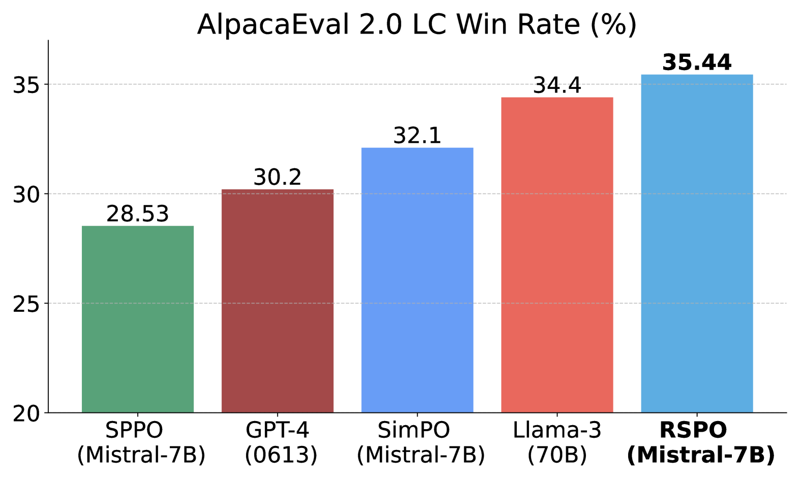
Figure 1: Our Regularized Self-Play Policy Optimization (RSPO) with Mistral-7B-Instruct outperforms Llama-3-70B, SimPO (Meng et al., 2024), and SPPO (Wu et al., 2024) in AlpacaEval-2 with length-controlled (LC) win rate.

Large Language Models (LLMs) recently have obtained remarkable capabilities to accomplish a range of tasks (Jiang et al., 2023a; Dubey et al., 2024; DeepSeek-AI et al., 2025), generating more desirable and helpful content following the user’s intention. One of the most important methods to align LLMs with human intentions is Reinforcement Learning from Human Feedback (RLHF), maximizing a preference-based reward penalized by a reverse KL regularization term of LLM policy and a supervised fine-tuning (SFT) reference model (Christiano et al., 2017; Ouyang et al., 2022; Rafailov et al., 2024; Azar et al., 2024; Xiong et al., 2024). This regularization is crucial in RLHF to prevent over-optimization, which has been extensively studied and even extended beyond KL divergence (Go et al., 2023; Huang et al., 2024).

Self-play is a general line of works conducting iterative self-competition of models, which has been demonstrated as an effective approach for improving AI systems (Goodfellow et al., 2020; Wang et al., 2022), particularly in strategic decision-making problems (Silver et al., 2016; Heinrich and Silver, 2016; Pinto et al., 2017; Brown and Sandholm, 2018). In the human alignment of LLMs, self-play recently started to be used and has shown superior empirical performance than other iterative RLHF methods on benchmarks like AlpacaEval and Arena-Hard Evaluation (Dubois et al., 2024; Jiang et al., 2024; Wu et al., 2024; Rosset et al., 2024). By formulating the preference optimization problem as a two-player game, self-play alignment methods seek to identify a Nash Equilibrium (NE) of the game in which utility is determined by a general preference model (Munos et al., 2023; Calandriello et al., 2024; Azar et al., 2024). This NE is regarded as the most aligned LLM policy, achieved without Bradley-Terry (BT) assumption (David, 1963).

Despite the significant empirical improvements achieved through self-play, the impact of regularization to the reference policy—commonly used in RLHF to mitigate over-optimization—has received insufficient investigation in self-play alignment. Most existing self-play methods lack explicit regularization (Swamy et al., 2024; Rosset et al., 2024; Wu et al., 2024; Wang et al., 2024; Gao et al., 2024). In practice, unregularized self-play is also susceptible to over-optimization, particularly when the preference model is misspecified. While some approaches incorporate regularization, they are typically constrained to a reverse KL divergence penalty that restricts deviations from the reference policy (Munos et al., 2023; Zhang et al., 2024).

In this paper, we introduce a generalized framework for incorporating diverse regularization methods into self-play alignment, termed Regularized Self-Play Policy Optimization (RSPO). RSPO offers a simple way to apply various regularization strategies in self-play by directly adding the regularization term to the loss function, while maintaining last-iterate convergence to the NE of the corresponding regularized preference optimization game. Empirical analysis reveals distinct effects of different regularization methods: forward KL regularization reduces the response length in RSPO, whereas reverse KL regularization significantly enhances the raw win rate. Consequently, we adopt a linear combination of forward and reverse KL divergences, yielding a substantial improvement over the unregularized self-play alignment method, SPPO (Wu et al., 2024), on various benchmarks. Particularly on AlpacaEval-2, RSPO outperforms SPPO with a $6.9$ percentage points increase in length-controlled win rate (LCWR) and an $18$ percentage point LCWR improvement over the base model, Mistral-7B-Instruct. Furthermore, we offer an analysis of response diversity that regularization also promotes greater diversity. In summary, regularization plays a crucial role in self-play alignment, significantly improving both the quality and diversity of responses in previously unregularized self-play methods.

2 Related Work

Azar et al. (2024) introduced the first approach for optimizing general preference models. Nash-MD (Munos et al., 2023) pioneered the application of self-play to general preference optimization by framing it as a two-player game. Subsequent methods have either focused on learning the NE of the original unregularized game (e.g. (Swamy et al., 2024; Wu et al., 2024; Rosset et al., 2024; Wang et al., 2024)) or the NE of a reverse-KL-regularized preference optimization game (e.g. (Munos et al., 2023; Calandriello et al., 2024; Zhang et al., 2024)). In contrast, our work explores a broader class of divergence-based regularization techniques for self-play alignment.

We emphasize the distinction between our self-play approach and self-play methods based on pairwise comparisons, which construct loss functions by leveraging the difference in policy logits between preferred and rejected responses—such as Direct Policy Optimization (DPO) (Rafailov et al., 2024) and Identity Policy Optimization (IPO) (Calandriello et al., 2024). Direct Nash Optimization (DNO) (Rosset et al., 2024) and Iterative Nash Policy Optimization (INPO) (Zhang et al., 2024) follow the Mirror Descent (MD) update (Beck and Teboulle, 2003) while computing loss using pairwise comparisons. However, optimizing such pairwise-comparison-based losses can lead to only an increase in the relative likelihood gap without necessarily enhancing the absolute probability of the preferred response (Pal et al., 2024). In contrast, our method directly approximates the MD update by converting MD as a reinforcement learning problem, thereby circumventing the limitations of pairwise comparison-based approaches.

Online iterative RLHF, which incorporates a reliable reward or preference model—including self-play—functions as a self-improving framework by iteratively generating new data using models and optimizing policies based on this data (Schulman et al., 2017; Ouyang et al., 2022; Bai et al., 2022; Touvron et al., 2023; Dong et al., 2024). Moreover, extending powerful offline methods such as Direct Preference Optimization (DPO) to iterative frameworks has led to significant performance gains (Xu et al., 2023; Liu et al., 2023; Tran et al., 2023; Dong et al., 2024; Calandriello et al., 2024; Pang et al., 2024; Xiong et al., 2024; Guo et al., 2024; Tajwar et al., 2024; Cen et al., 2024; Xie et al., 2024). In contrast, our work investigates general preference optimization through self-play from a game-theoretic perspective, shifting the objective from conventional RL optimization to the computation of NE.

3 Preliminaries

We denote a prompt as $x$, a response as $y$, and a LLM policy as $\pi(y|x)$, where $\pi(\cdot|x)\in\Delta_{\mathcal{Y}}$, $\mathcal{X}$ is the set of all prompts and $\mathcal{Y}=\{y^{0},y^{1},\cdots\}$ is the set of all responses. We denote the probability simplex over the responses given a specific prompt as $\Delta_{\mathcal{Y}}$. We parametrize the LLM policy $\pi$ as $\pi_{\theta}$. The reference policy is an LLM denoted as $\mu\in\Delta^{\mathcal{X}}_{\mathcal{Y}}$. For notational brevity, we remove the dependence of policy $\pi$ and loss functions on the prompt $x$ throughout the paper.

3.1 Game-Theoretic Preference Optimization

We study the preference optimization problem in an online setting by formulating it as a two-player max-min game, as studied in previous self-play works (Wu et al., 2024). The players are two LLMs whose strategies are LLM policies, denoted as max-player $\pi$ and min-player $\pi^{\prime}$. The utility of the max-player is the preference:

$$u(\pi;\pi^{\prime})=\mathbb{P}(\pi\succ\pi^{\prime})\overset{\text{def}}{=}\mathbb{E}_{y\sim\pi,y^{\prime}\sim\pi^{\prime}}[\mathbb{P}(y\succ y^{\prime})],$$ (1)

where $u:\Delta^{\mathcal{X}}_{\mathcal{Y}}\times\Delta^{\mathcal{X}}_{\mathcal{Y}}\rightarrow\mathbb{R}$ is linear in $\pi$ and $\pi^{\prime}$; $\mathbb{P}:\mathcal{X}\times\mathcal{Y}\times\mathcal{Y}\rightarrow[0,1]$ is a general preference model that quantifies the preference of $y$ over $y^{\prime}$ given a prompt. We extend the notation $\mathbb{P}(y\succ\pi^{\prime})=\mathbb{E}_{y^{\prime}\sim\pi^{\prime}}[\mathbb{P}(y\succ y^{\prime})]$ for any response $y$. The objective is finding a NE policy $\pi^{*}$ of the preference model:

$$(\pi^{*},\pi^{*})=\arg\max_{\pi}\min_{\pi^{\prime}}\mathbb{P}(\pi\succ\pi^{\prime}).$$ (2)

Therefore, an NE strategy $\pi^{*}$ is an LLM that can generate the most preferred responses in expectation, thus achieving human alignment based on the preference model.

Existing game-theoretic self-play methods solve this NE following Algorithm 1 (Wu et al., 2024; Swamy et al., 2024; Zhang et al., 2024; Wang et al., 2024). Specifically, the policy is first initialized as $\pi_{0}=\mu$. Then in each iteration $t$, the opponent is set to be the last-iterate policy $\pi_{t}$ (the reason why it is called self-play), and the responses are sampled from $\pi_{t}$ (Line 4). The pairwise preferences of the sampled responses are collected using the preference model $\mathbb{P}$ (Line 5). The policy parameters are updated by minimizing a specified loss function $\mathcal{L}(\theta;\mathbb{P})$ based on preferences over responses (Line 6). The loss function $\mathcal{L}(\theta;\mathbb{P})$ is dependent on the inherent online learning method.

3.2 Preference Optimization via Multiplicative Weights Update

An effective self-play method to solve the preference optimization game in Equation˜2 is Self-Play Policy Optimization (SPPO) (Wu et al., 2024). SPPO derives its loss function from the iterative no-regret learning algorithm, Multiplicative Weights Update (MWU) (Freund and Schapire, 1997). Specifically in a game setting, denote learning rate as $\eta$, and normalization constant $Z(\pi_{t})$. In any iteration $t$, the policy update $\forall y\in\mathcal{Y}$ is

$$\pi_{t+1}(y)=\pi_{t}(y)\cdot\frac{\exp\Big{(}\eta\mathbb{E}_{y^{\prime}\sim\pi_{t}}[u({y};y^{\prime})]\Big{)}}{Z(\pi_{t})},$$ (3)

where $u(y;y^{\prime})$ is the utility function defined in Equation (1), with $y$ treated as a pure strategy.

The practical loss function of SPPO for policy update in each iteration $t$ is the square error between LHS and RHS in Equation˜3 at a logarithmic scale, defined as

$$\mathcal{L}_{\text{SPPO}}(\theta)=\mathbb{E}_{y\sim\pi_{t}}\Big{[}\log\frac{\pi_{\theta}(y)}{\pi_{t}(y)}-\Big{(}\eta\mathbb{P}({y}\succ\pi_{t})-\log Z(\pi_{t})\Big{)}\Big{]}^{2}.$$ (4)

SPPO converges to the NE of the preference optimization game in Equation˜2. However, after running multiple iterations, the deviation of the policy $\pi_{\theta}$ from $\mu$ can be large. Such deviation is particularly problematic when the preference model is only accurate at evaluating responses sampled from the reference policy (Munos et al., 2023). Furthermore, in aligning LLMs in practice, the preference model is typically a surrogate $\hat{\mathbb{P}}$, such as PairRM (Jiang et al., 2023b), which may be misspecified at some out-of-distribution responses and inaccurate due to estimation error or limited model expressiveness (e.g., PairRM is only a 0.4B model), causing over-optimization problem. Regularizing the policy optimization to a reference SFT model, which is typically trained on high-quality data (Ouyang et al., 2022), can mitigate the problem. We provide a synthetic example in Appendix C.1 to demonstrate the problem.

3.3 Regularized Preference Optimization Game with Reference Policy

To address the regularization in self-play, we adopt the objective in Nash Learning from Human Feedback (Munos et al., 2023), and extend the KL divergence regularization to a general regularization function, to penalize the deviation from reference policy. We define a convex regularization function $R:\Delta^{\mathcal{X}}_{\mathcal{Y}}\times\Delta^{\mathcal{X}}_{\mathcal{Y}}\rightarrow(-\infty,\infty)$, where $R(\pi,\mu)$ measures the distance between $\pi$ and the reference model $\mu$, such as KL divergence $D_{\text{KL}}(\pi\|\mu)$. Denote regularization temperature as $\tau$, the objective becomes to optimize a regularized preference model by solving the NE $(\pi^{*},\pi^{*})$ of the regularized game, where the utility of max player is still $u(\pi;\pi^{\prime})=\mathbb{P}(\pi\succ\pi^{\prime})$:

$$\arg\max_{\pi}\min_{\pi^{\prime}}\mathbb{P}(\pi\succ\pi^{\prime})-\tau R(\pi,\mu)+\tau R(\pi^{\prime},\mu).$$ (5)

We provide proof of the existence and uniqueness of this NE in Appendix A.2. Various methods leverage Mirror Descent (MD) to find a regularized NE in Equation˜5 (Munos et al., 2023; Calandriello et al., 2024; Zhang et al., 2024; Wang et al., 2024), based on its last-iterate convergence.

However, these MD-based methods are only compatible with the reverse KL divergence regularizer. Nash-MD addresses the reverse KL regularization of $\pi$ and $\mu$ using a geometric mixture policy $\pi_{t}^{\mu}$ defined as $\pi_{t}^{\mu}(y)={\pi_{t}(y)^{1-\eta\tau}\mu(y)^{\eta\tau}}/{\sum_{y^{\prime}}\pi_{t}(y^{\prime})^{1-\eta\tau}\mu(y^{\prime})^{\eta\tau}}$ (Munos et al., 2023), which updates policy as:

$$\pi_{t+1}=\arg\min_{\pi}-\eta\langle\pi,\partial_{\pi}u(\pi_{t};{\pi^{\mu}_{t}})\rangle+D_{\text{KL}}(\pi,\pi_{t}^{\mu}).$$ (6)

While the LLMs optimized via self-play exhibit significant improvement (Wu et al., 2024; Wang et al., 2024; Zhang et al., 2024), they all have limited regularization of $\pi$ and $\mu$. They either completely lack explicit regularization or only employ reverse KL divergence, imposing only a narrow form of regularization. The potential benefits of alternative regularization, such as adopting other $f$-divergences than reverse KL, remain unexplored.

4 Regularized Self-Play Policy Optimization

We propose a simple, general, and theoretically sound framework of self-play alignment, namely Regularized Self-Play Policy Optimization (RSPO). Intuitively, RSPO can be understood as an extension of SPPO with an external regularization term, allowing different regularization strategies to be employed. The loss function of RSPO $\mathcal{L}_{\text{RSPO}}$ is defined as the sum of a mean-squared self-play loss, denoted as $\mathcal{L}_{\text{SP}}$, and a weighted regularization term:

$$\mathcal{L}_{\text{RSPO}}(\theta;G,B,R)\overset{\text{def}}{=}\mathbb{E}_{y\sim\pi_{t}}\Big{[}\log\frac{\pi_{\theta}(y)}{\pi_{t}(y)}-\eta\Big{(}G({y},\pi_{t},\mu)-B(\pi_{t},\mu)\Big{)}\Big{]}^{2}\hbox{\pagecolor{cyan!20}$+\lambda R(\pi_{\theta},\mu)$},$$ (7)

where $G({y},\pi_{t},\mu)$, $B(\pi_{t},\mu)$, and $R(\pi_{\theta},\mu)$ are configurable components. First, $G:\mathcal{Y}\times\Delta^{\mathcal{X}}_{\mathcal{Y}}\times\Delta^{\mathcal{X}}_{\mathcal{Y}}\rightarrow(-\infty,\infty)$ defines the update direction of $\pi_{\theta}$, which can be set as the gradient of a utility function to guide the policy update towards increasing the utility. Second, the baseline function $B:\Delta^{\mathcal{X}}_{\mathcal{Y}}\times\Delta^{\mathcal{X}}_{\mathcal{Y}}\rightarrow(-\infty,\infty)$ is for variance-reduction for $G$, similar to the baseline in REINFORCE (Williams, 1992). Lastly, $R:\Delta^{\mathcal{X}}_{\mathcal{Y}}\times\Delta^{\mathcal{X}}_{\mathcal{Y}}\rightarrow\mathbb{R}$ is the regularization function. The coefficient $\lambda$ is the regularization temperature. The first Mean Square Error term in Equation˜7 can be interpreted as a self-play loss of conducting exponentiated gradient descent (Beck and Teboulle, 2003).

RSPO offers a simple way to introduce regularization into self-play alignment with only an additional term in the loss. Using RSPO, self-play can be regularized by simply adding a term $R$ to the self-play loss functions. For example, to regularize SPPO (Equation˜4), we can leverage RSPO loss function (Equation˜7) by setting appropriate $G$ and $B$, and directly adding an additional term of $R$ to the loss function of SPPO. Therefore, RSPO offers the simplicity and flexibility to incorporate various regularization methods into self-play-based preference optimization methods.

Furthermore, RSPO is a generalized and versatile framework that makes the import of regularization into existing self-play methods more efficient. We show in Section 4.1 that RSPO can generalize existing self-play methods with $\mathcal{L}_{\text{SP}}$ and without external regularization $R$. Thus, regularizing existing methods requires no change to their loss functions or hyperparameters, but simply adding an external regularization to their loss function and tuning the temperature $\lambda$.

We provide the theoretical guarantee for RSPO in Section 4.2 by showing that RSPO is the RL implementation of a specific type of Mirror Descent. Given a specific regularizer $R$, RSPO has a last-iterate convergence to the NE of the corresponding regularized game. We also introduce the implementation details of RSPO specifically for preference optimization (Equation˜5) in Section 4.3.

4.1 Generalizing Existing Self-Play Methods

We show that existing methods have loss functions equivalent to RSPO without external regularization: $\mathcal{L}_{\text{RSPO}}(\theta;G,B,R=0)$. First of all, unregularized self-paly method SPPO (Wu et al., 2024), has loss function in Equation˜4 satisfying:

$$\mathcal{L}_{\text{SPPO}}(\theta)=\mathcal{L}_{\text{RSPO}}\bigg{(}\theta;G=\mathbb{P}(y\succ\pi_{t}),B=\frac{1}{2},R=0\bigg{)}.$$ (8)

Other unregularized self-play methods following the preference-based exponential update in Equation˜3 can also be generalized by $\mathcal{L}_{\text{SP}}$, and thus can be regularized by simply adding regularization term to the loss functions. Based on the same exponential update rule as in SPPO, SPO (Swamy et al., 2024) is equivalent to updating policy with the loss in Equation˜8. Magnetic Policy Optimization (Wang et al., 2024), despite incorporating regularization in the policy update, periodically update $\mu=\pi_{t}$. Consequently, it inherently follows update in Equation˜3 while incorporating multiple policy updates within each iteration, following the approach of (Tomar et al., 2020).

In addition, even existing regularized methods can be generalized by $\mathcal{L}_{\text{RSPO}}$ without external regularization. Mirror Descent methods including Online Mirror Descent and Nash-MD (implemented with RL) have direct connection to RSPO (the detailed derivations are provided in Appendix A.1):

$$\nabla_{\theta}\mathcal{L}_{\text{Nash-MD}}(\theta)=\nabla_{\theta}\mathcal{L}_{\text{RSPO}}\bigg{(}\theta;G=\mathbb{P}(y\succ\pi_{t}^{\mu})-\tau\log\frac{\pi_{t}(y)}{\mu(y)},B=\frac{1}{2},R=0\bigg{)}.$$ (9)

This equivalence fundamentally arises from the well-established connection between the reinforcement learning (RL) policy gradient and the gradient of a quadratic loss function, as explored in various works (Haarnoja et al., 2018; Tomar et al., 2020; Malkin et al., 2022). We summarize the generalization of RSPO in Table 3. Therefore, our generalized loss framework RSPO enables to even add extra regularization to existing regularized self-play methods.

4.2 Theoretical Results

In this section, we examine the theoretical properties of RSPO, with a particular emphasis on its convergence guarantee. We adopt Mirror Descent (MD) as the foundational framework, given its well-established last-iterate convergence to the NE in game-solving.

We build upon Magnetic Mirror Descent (MMD) (Sokota et al., 2022), a specialized variant of MD that guarantees convergence to a reverse-KL-regularized NE. To generalize beyond reverse-KL regularization, we introduce Generalized Magnetic Mirror Descent (GMMD), which can accommodate a broader class of regularization techniques. By demonstrating that optimizing the RSPO loss is equivalent to performing reinforcement learning (RL) within the GMMD framework, we establish a formal connection between RSPO and GMMD. This connection ensures the last-iterate convergence of RSPO to the NE of the corresponding regularized game.

Tabular GMMD. Denote the utility function of the game as $U$, define $G$ as the element of the gradient vector of $U$: $G(y;\pi^{\prime})\overset{\text{def}}{=}\partial_{\pi(y)}U(\pi;\pi^{\prime})$. In other words, $\partial_{\pi}U(\pi;\pi^{\prime})=(G(y^{0};\pi^{\prime}),\cdots,G(y^{|\mathcal{Y}|};\pi^{\prime}))^{\top}\in\mathbb{R}^{|\mathcal{Y}|}$. Then in iteration $t$, GMMD updates policy as

$$\pi_{t+1}=\arg\min_{\pi}-\eta\mathbb{E}_{\pi}[G(y;\pi_{t})]+B_{\psi}(\pi;\pi_{t})+\tau R(\pi,\mu),$$ (10)

where $\tau$ is regularization temperature, $R$ is a general regularization function, serving as a “magnet” to attract $\pi$ to $\mu$ during policy updating. $B_{\psi}$ is the Bregman Divergence generated by a convex potential function $\psi$ (Bregman, 1967).

Notably, the vanilla Magnetic Mirror Descent limits $R$ to be the same regularization method of $\pi$ and $\pi_{t}$, i.e., $R=B_{\psi}$ (Sokota et al., 2022, Section 3.2); whereas in this paper we aim at a general regularizer of $\pi$ and $\mu$, which could be different from $B_{\psi}$, and study the effects of different regularizations methods.

Proposition 4.1 (Last-iterate Convergence).

If $R(\cdot,\mu)$ is $1$-strongly convex relative to $\psi$, $\eta\leq\tau$, and $U$ is linear, then policy updated by GMMD in Equation˜10 has last-iterate convergence to the following regularized NE:

$$\max_{\pi}\min_{\pi^{\prime}}U(\pi;\pi^{\prime})-\tau R(\pi,\mu)+\tau R(\pi^{\prime},\mu).$$ (11)

Proposition 4.1 is a direct application of Theorem 3.4 by Sokota et al. (2022), which guarantees the last-iterate convergence of GMMD to the NE of a regularized game. We provide the proof in Appendix A.3.

Deep RL Implementation of GMMD. To adapt GMMD to preference optimization problems, RL techniques are commonly employed as practical implementations, as for many MD update (Tomar et al., 2020; Munos et al., 2023; Wang et al., 2024). Define the loss function of conducting GMMD in preference optimization as

$$\mathcal{L}_{\text{GMMD}}(\theta)\overset{\text{def}}{=}-\eta\mathbb{E}_{\pi_{\theta}}\big{[}G(y;\pi_{t})\big{]}+D_{\text{KL}}(\pi_{\theta}||\pi_{t})+\tau R(\pi_{\theta},\mu).$$ (12)

Here, we set the Bregman divergence to Reverse KL in preference optimization as in previous works (Munos et al., 2023; Zhang et al., 2024). The gradient estimation of $\mathcal{L}_{\text{GMMD}}(\theta)$ for policy updates is required since the expectation in the first term is dependent on $\pi_{\theta}$. Following Policy Gradient theorem (Sutton et al., 1999), then we have

$$\nabla_{\theta}\mathcal{L}_{\text{GMMD}}(\theta)=\mathbb{E}_{y\sim\pi_{\theta}}\bigg{[}\nabla_{\theta}\log\pi_{\theta}(y)\bigg{(}-\eta G(y;\pi_{t})+\log\frac{\pi_{\theta}(y)}{\pi_{t}(y)}+B\bigg{)}\bigg{]}+\tau\nabla_{\theta}R(\pi_{\theta},\mu),$$ (13)

where $B$ is a baseline function to reduce the variance as in REINFORCE (Williams, 1992). We set $B$ independent to $\theta$ so that adding $B$ does not affect the value of Equation˜12, due to $\mathbb{E}_{y\sim\pi_{\theta}}[\nabla_{\theta}\log\pi_{\theta}(y)\cdot\eta B]=\eta B\nabla_{\theta}\mathbb{E}_{y\sim\pi_{\theta}}[1]=0$.

We follow SPPO to replace the samples $y\sim\pi_{\theta}$ with $y\sim\pi_{t}$ directly since they are equivalent while computing the loss before updating, and rewrite the loss equivalent to GMMD:

$$\nabla_{\theta}\mathcal{L}_{\text{GMMD}}(\theta)=\nabla_{\theta}\Bigg{(}\frac{1}{2}{\mathbb{E}_{{y\sim\pi_{t}}}\Big{[}-\eta G(y;\pi_{t})+\log\frac{\pi_{\theta}(y)}{\pi_{t}(y)}{+\eta B}\Big{]}^{2}}+\tau R(\pi_{\theta},\mu)\Bigg{)}.$$ (14)

Therefore, according to Equation˜14, RSPO is equivalent to the RL implementation of GMMD since the RHS of the Equation˜14 is RSPO loss up to multiplying a constant.

4.3 Implementation for Preference Optimization

In this section, we introduce the implementation of RSPO. We set the update direction $G$ to be the gradient of the preference against $\pi_{t}$, $\forall y\in\mathcal{Y}$:

$$G({y},\pi_{t},\mu)=\partial_{\pi(y)}\mathbb{P}(\pi\succ\pi_{t})=\mathbb{P}(y\succ\pi_{t}).$$ (15)

As for baseline function $B$, we set $B=\tfrac{1}{2}$ following Nash-MD and SPPO. In theory, $B$ helps minimize the variance of $G$ the most when $B=\mathbb{E}_{y\sim\pi_{t}}[G(y,\pi_{t},\mu)]$. But in preference optimization, due to the typically small minibatch size, the estimation error of the mean of $G$ could be large, leading to additional estimation error of the loss. Thus, we also set the baseline value for variance reduction to be a constant $\tfrac{1}{2}$, the mean value of $G$ when the algorithm is converged.

Specifically, we execute Algorithm 1 by applying the following RSPO loss with any regularization $R$ of interest:

$$\mathcal{L}_{\text{RSPO}}\big{(}\theta;G=\mathbb{P}(y\succ\pi_{t}),B=\tfrac{1}{2},R\big{)}=\mathcal{L}_{\text{SPPO}}+\lambda R(\pi_{\theta},\mu).$$ (16)

Therefore, we can directly use the off-the-shelf self-play alignment method SPPO to implement RSPO. The only modification required is to add the regularization to the SPPO loss. Various divergences for regularization are implemented, as discussed in Appendix B.3.

For completeness, we provide the convergence guarantee for this instance of RSPO to the Nash equilibrium of the regularized preference optimization game as follows (Proof in Appendix A.4).

Corollary 4.2.

Self-play following Algorithm 1 with the RSPO loss function in Equation˜16 and regularizer $R$ satisfying the assumption in Proposition 4.1, has last-iterate convergence to the NE of the regularized preference optimization game, as described in Equation˜5.

RSPO guarantees NE convergence while allowing flexible regularization strategies, making it a robust extension of self-play optimization. In summary, the proposed RSPO framework provides a generalized approach that simplifies the incorporation of regularization into existing self-play methods while maintaining theoretical soundness.

5 Experiments

Methods (Base Model: Mistral-7B-Instruct)	AlpacaEval-2 LCWR ($\%$)	Arena-Hard Auto-v0.1	MT-Bench
Mistral-7B-Instruct (Jiang et al., 2023a)	17.1	12.6	7.51
Snorkel (Iterative DPO) (Tran et al., 2023)	26.4	20.7	7.58
SPPO Iter3 (Wu et al., 2024)	28.5	19.2	7.59
SimPO (Meng et al., 2024)	32.1	21.0	7.60
RSPO (IS-For.+Rev.) Iter3	35.4	22.9	7.75

Table 1: Performance of existing methods, and our strongest model: RSPO with Importance-Sampling-based Forward KL ($\lambda_{1}=0.1$) + Reverse KL ($\lambda_{2}=0.5$) divergence as regularization, on AlpacaEval-2 and Arena-Hard-Auto-v0.1.

In this section, we answer the following important questions of regularization in the self-play alignment of Large Language Models (LLMs) by testing on various popular benchmarks:

• Q1: Does regularization improve the performance of self-play alignment of LLMs (Sec. 5.1)?

• Q2: Which regularization method is the most effective in self-play alignment (Sec. 5.2)?

• Q3: What additional advantages can be derived from utilizing regularization in self-play (Sec. 5.3)?

Experiment Setup. We investigate our methods mainly on benchmarks AlpacaEval (Dubois et al., 2024), Arena-Hard (Li et al., 2024), and MT-Bench (Zheng et al., 2023). We follow the experiment setup of SPPO and Snorkel-Mistral-PairRM-DPO (Snorkel) (Tran et al., 2023) to examine our regularization methods, where Snorkel is based on iterative DPO and has achieved strong performance on AlpacaEval. Our reference policy model is Mistral-7B-Instruct-v0.2. Since iterative self-play methods require no response data for training, we only use the prompts of the Ultrafeedback dataset (Cui et al., 2023), whose size is $\sim 60$K. Following SPPO and Snorkel, we split the prompts into three subsets and use only one subset per iteration to prevent over-fitting. To understand the later-iterate performance of self-play, in section 5.1, we also train on the single fold of the prompts iteratively. We use a 0.4B response-pair-wise preference model PairRM (Jiang et al., 2023b), evaluated as comparable to $10\times$ larger reward/preference models (Cui et al., 2023). We investigate the effect of regularization mainly via AlpacaEval-2.0, where the main metric is length-controlled win rate (LCWR).

Implementations and Baselines. The implementation of self-play methods follows Algorithm 1. In each iteration, given response-pair-wise preference from PairRM and $K=5$ number of response samples from the current policy, we estimate the policies’ preference $\mathbb{P}(\pi\succ\pi_{t})$ and regularization via Monte-Carlo estimation to compute the loss function. We replicate the SPPO with the default hyper-parameters and extend it to $9$ iterations. We implement RSPO as described in Corollary˜4.2. The implementation of regularizations in RSPO is demonstrated in Appendix B.3 using the $K$ samples. We report some of the baseline results from the previous papers, including SPPO, Snorkel (Mistral-PairRM-DPO) (Tran et al., 2023), Mistral-7B (Instruct-v0.2) (Jiang et al., 2023a), iterative DPO by Wu et al. (2024), and SimPO Meng et al. (2024). Since the SPPO paper only provides results across $3$ iterations (Wu et al., 2024), we replicate SPPO as an important baseline to study the performance across more than $3$ iterations.

5.1 Effectiveness of Regularization

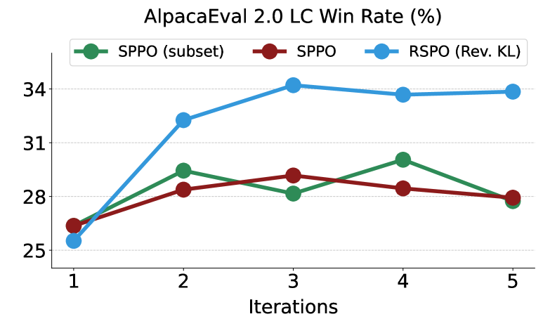
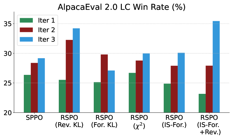
Figure 2: Left: LC win rate across iterations for unregularized self-play method SPPO, SPPO trained on a subset of the data (SPPO (subset)), and reverse-KL-regularized RSPO (RSPO (Rev. KL)). The base model is Mistrial-7B. SPPO starts to degrade after $3$ iterations. Right: LC win rate of SPPO and RSPO with different regularization methods. From left to right regularization methods: Reverse KL ($\lambda=0.5$), Forward KL ($\lambda=1.0$), Chi-Squared ($\lambda=0.1$), Importance-Sampling Forward KL ($\lambda=0.1$), Forward and Reverse KL linear combination ($\lambda_{1}=0.1$, $\lambda_{2}=0.5$). RSPO outperforms unregularized self-play (SPPO) significantly.

In this section, we assess the effectiveness of regularization primarily by comparing the performance of unregularized and regularized self-play methods. We first examine the over-optimization issue inherent in practical self-play preference optimization by extending the execution of SPPO to Iteration 5. As depicted in Figure 2, a decline in performance appears during the later iterations of SPPO. We hypothesize that this behavior arises from the practical challenges associated with a misspecified preference model, as the signals driving policy updates in SPPO rely only on the preference model.

In Table 2, we further contrast the unregularized self-play method, SPPO, and other iterative methods with the best RSPO, namely RSPO (For.+Rev.). The regularization is a linear combination of Forward KL and Reverse KL divergence with coefficients $0.1$ and $0.5$, respectively. The comparative results reveal that regularization enhances the SPPO win rate from $31.02\%$ to $38.31\%$, and the LC win rate increases from $28.53\%$ to $35.44\%$ in iteration $3$. Notably, in the first iteration, reg. SPPO exhibits a slightly lower LC win rate, potentially attributable to the influence of strong regularization. However, subsequent iterations show a marked improvement, with the LC win rate of reg. SPPO increases by up to $7.53\%$ within a single iteration. In summary, the findings in Table 2 underscore the effectiveness of regularization in self-play optimization.

Additionally, to rule out the possibility of insufficient iterations affecting performance, we report the best result among nine iterations of our replicated SPPO in Table 2, denoted as "SPPO $\leq 9$". SPPO $\leq 9$ consistently underperforms the RSPO result at iteration $3$. These observations emphasize that even extended training under the unregularized framework fails to match the performance gains achieved through regularization, thereby affirming the critical role of regularization in self-play methodologies for preference optimization.

Model	AlpacaEval 2.0
	LC Win Rate	Win Rate	Avg. Len
Mistral-7B	17.11	14.72	1676
Snorkel	26.39	30.22	2736
SimPO	32.1	34.8	2193
DPO Iter1	23.81	20.44	1723
DPO Iter2	24.23	24.46	2028
DPO Iter3	22.30	23.39	2189
SPPO Iter1	24.79	23.51	1855
SPPO Iter2	26.89	27.62	2019
SPPO Iter3	28.53	31.02	2163
SPPO $\leq$ 9	29.17	29.75	2051
RSPO Iter1	23.16	21.06	1763
RSPO Iter2	27.91	27.38	1992
RSPO Iter3	35.44	38.31	2286

Regularization	Iteration	AlpacaEval 2.0
		LCWR $\uparrow$	Self-BLEU $\downarrow$
$\times$	1	24.79	0.751
	2	26.89	0.754
	3	28.53	0.758
IS-Forward KL + Reverse KL	1	23.16	0.747
	2	27.91	0.743
	3	35.44	0.714
Reverse KL	1	25.52	0.747
	2	32.26	0.730
	3	34.21	0.691
IS-Forward KL	1	24.88	0.756
	2	27.9	0.759
	3	30.09	0.760
$\chi^{2}$	1	26.7	0.745
	2	28.78	0.740
	3	29.97	0.739

Table 2: Left: Comparisons of iterative methods with reference models Mistral-7B (Instruct-v0.2). SPPO $\leq$ 9 represents the best results among the $9$ iterations of SPPO. Here, the Regularized SPPO (RSPO) is regularized by the linear combination of Forward KL and Reverse KL divergence, i.e. RSPO (For. + Rev.), where the regularization temperatures are $0.1$ and $0.5$, respectively. Right: Response diversity of SPPO with different regularization methods using Self-BLEU score. The regularization temperatures are the same as in Figure 2 (Right). A lower Self-BLEU score means a higher diversity of the sampled responses. Regularization methods involving Reverse KL resulted in higher diversity of the responses.

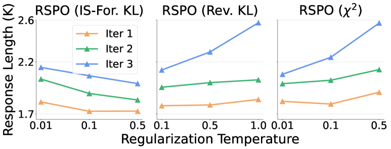
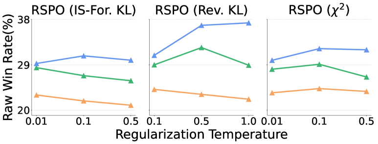
Figure 3: Ablation study of regularization temperature $\lambda$ conducted on AlpacaEval 2.0. We evaluate how the average response length and raw WR are affected by the regularization temperature.

5.2 Impact of Different Regularizations

We then study the effect of applying different regularization $R$ in RSPO. To obtain a well-regularized self-play, the tuning of regularization temperature $\lambda$ is necessary. An ablation study of the regularization temperature of different methods is shown in Figure 3. According to the figure, the response length increases along with the temperature in reverse KL divergence and Chi-square divergence regularized RSPO. Meanwhile, the length is decreased with stronger regularization via Forward KL divergence, which was implemented using importance sampling. This result underscores the distinct effects of different regularization strategies. In particular, the raw win rate analysis highlights reverse KL divergence as a crucial factor in enhancing self-play performance. Given that forward KL divergence tends to reduce response length while reverse KL divergence yields significant improvements, we adopt a linear combination of both. This approach is designed to balance their complementary effects, ultimately optimizing for a higher LCWR (RSPO (IS-For. + Rev.) in Figure 2 RHS).

In Figure 2 (Right), we show the results of win rate and LCWR in AlpacaEval 2.0 of different regularizations. Only vanilla Forward KL decreases the win rate of SPPO. The regularizations that consists of Reverse KL including RSPO (Rev. KL) and RSPO (For.+Rev.) have shown significant improvement in win rates compared to vanilla SPPO. In particular, the results of RSPO (For.+Rev.) demonstrate the largest improvement between iterations, achieving the best LCWR.

We study the effect of applying different regularization $R$ in RSPO. In Figure 2 (Right), we show the results of win rate and average response length on AlpacaEval 2.0. Among different regularizations, only Forward KL decreases the win rate of SPPO. The regularizations that consist of Reverse KL including RSPO (Rev. KL) and RSPO (For.+Rev.) have shown significant improvement in win rates compared to vanilla SPPO. In particular, the results of RSPO (For.+Rev.) demonstrate the largest improvement between iterations. We test the best RSPO model on different benchmarks in Table 1, and observe that the proposed method RSPO with proper external regularization achieves superior performance than unregularized self-play and iterative methods like SPPO and iterative DPO, as well as the strong offline alignment method SimPO.

5.3 Response Diversity

We demonstrate an additional advantage introduced by regularization, which is the diversity of the response. We first provide a motivating example with synthetic data in Appendix C.2, which shows that the unregularized self-play may converge to a collapsed response when multiple equally good responses exist. On the contrary, RSPO with maximum entropy regularization can recover all high-reward responses.

For LLMs, we investigate the diversity of generations by estimating the variability of the responses. We use the Self-BLEU (Zhu et al., 2018) score, where a lower score implies higher response diversity. We take the first $200$ tokens of each of the $16$ generated responses using the prompts of AlpacaEval.

The trend of Self-BLEU scores presented in Table˜2 (Right) show that applying RSPO with Reverse KL increases response diversity the most, as well as the LCWRs of AlpacaEval 2.0. The application of Forward KL results in slightly less generation diversity than vanilla SPPO, but it still achieves better win rates. The win rates are the highest when Forward KL and Reverse KL are linearly combined for regularization, while the Self-BLEU scores imply that the response diversity is lower than when only Reverse KL is applied. These results highlight that applying regularization in self-play methods can improve test performance and the diversity of the generations simultaneously.

6 Conclusion

In this paper, we study the regularization in self-play by proposing a framework, namely Regularized Self-Play Policy Optimization (RSPO). Based on RSPO, we can apply different regularization functions for policy updates by adding the regularization term to the loss functions, which is still guaranteed to converge to the NE of the regularized preference optimization game. In the empirical assessments, we achieve significant improvement over the base model and unregularized self-play method, SPPO. We also empirically demonstrate that regularization promotes response diversity. These findings underscore the critical role of regularization as a fundamental component in optimizing self-play alignment.

Appendix A Proofs

In this section, we provide detailed derivations and proofs of propositions.

A.1 Proof of Equivalence between MD and RSPO

Proposition A.1.

Nash-MD and Online Mirror Descent [Munos et al., 2023, Section 6] can be seen as particular instances of our general Regularized Self-Play Policy Optimization (RSPO) (Equation˜7).

Proof.

In this section, we first provide derivations of Nash-MD and Online Mirror Descent to $\mathcal{L}_{\text{RSPO}}$ without external regularization.

Nash-MD practical loss satisfies that

$$\nabla_{\theta}\mathcal{L}_{\text{Nash-MD}}(\theta) =\mathbb{E}_{\begin{subarray}{c}y\sim\pi_{\theta},\\ y^{\prime}\sim\pi^{\mu}_{t}\end{subarray}}\Big{[}\nabla_{\theta}\log\pi_{\theta}(y)\Big{(}\mathbb{P}(y\succ y^{\prime})-\frac{1}{2}-\tau\log\frac{\pi_{\theta}(y)}{\mu(y)}\Big{)}\Big{]}$$ (17)

$$=\mathbb{E}_{\begin{subarray}{c}y\sim\pi_{\theta},\\ y^{\prime}\sim\pi^{\mu}_{t}\end{subarray}}\Big{[}\nabla_{\theta}\log\pi_{\theta}(y)\Big{(}\mathbb{P}(y\succ y^{\prime})-\frac{1}{2}-\tau\log\frac{\pi_{\theta}(y)}{\pi_{t}(y)}-\tau\log\frac{\pi_{t}(y)}{\mu(y)}\Big{)}\Big{]}$$ (18)

$$=\mathbb{E}_{y\sim\pi_{\theta}}\Big{[}\nabla_{\theta}\log\pi_{\theta}(y)\Big{(}\mathbb{P}(y\succ\pi^{\mu}_{t})-\frac{1}{2}-\tau\log\frac{\pi_{\theta}(y)}{\pi_{t}(y)}-\tau\log\frac{\pi_{t}(y)}{\mu(y)}\Big{)}\Big{]}$$ (19)

$$=\mathbb{E}_{y\sim\pi_{t}}\Big{[}\nabla_{\theta}\log\pi_{\theta}(y)\Big{(}\mathbb{P}(y\succ\pi^{\mu}_{t})-\frac{1}{2}-\tau\log\frac{\pi_{\theta}(y)}{\pi_{t}(y)}-\tau\log\frac{\pi_{t}(y)}{\mu(y)}\Big{)}\Big{]}$$ (20)

$$=\nabla_{\theta}\mathbb{E}_{y\sim\pi_{t}}\Big{[}\tau\log\frac{\pi_{\theta}(y)}{\pi_{t}(y)}-\Big{(}\mathbb{P}(y\succ\pi^{\mu}_{t})-\tau\log\frac{\pi_{t}(y)}{\mu(y)}-\frac{1}{2}\Big{)}\Big{]}^{2}/2$$ (21)

$$=\tau^{2}\nabla_{\theta}\mathbb{E}_{y\sim\pi_{t}}\Big{[}\log\frac{\pi_{\theta}(y)}{\pi_{t}(y)}-\frac{1}{\tau}\Big{(}\mathbb{P}(y\succ\pi^{\mu}_{t})-\tau\log\frac{\pi_{t}(y)}{\mu(y)}-\frac{1}{2}\Big{)}\Big{]}^{2}/2.$$ (22)

Equation˜17 is the definition of practical Nash-MD loss [Munos et al., 2023, Section 7]. Equation˜18 holds by adding an subtracting the same element $\log\pi_{t}(y)$. Equation˜19 holds due to $\mathbb{E}_{y^{\prime}\sim\pi_{t}^{\mu}}[\mathbb{P}(y\succ y^{\prime})]=\mathbb{P}(y\succ\pi_{t}^{\mu})$. Equation˜20 holds since in each iteration before updating, while computing the loss, $y\sim\pi_{\theta}$ is equivalent to $y\sim\pi_{t}$. The learning rate $\eta$ is originally omitted in the paper [Munos et al., 2023]. Here Nash-MD is generalized by $\mathcal{L}_{\text{RSPO}}$ with $\eta=\tfrac{1}{\tau}$ and $R=0$.

OMD is to execute $\arg\max_{\pi}\eta\mathbb{E}_{y\sim\pi}\left[\mathbb{P}(y\succ\pi_{t})-\tau\log\frac{\pi_{t}(y)}{\mu(y)}\right]-\text{KL}(\pi,\pi_{t})$. Therefore, the loss function of the OMD update satisfies

$$\nabla_{\theta}\mathcal{L}_{\text{OMD}}(\theta) =-\nabla_{\theta}\eta\mathbb{E}_{y\sim\pi_{\theta}}\left[\mathbb{P}(y\succ\pi_{t})-\tau\log\frac{\pi_{t}(y)}{\mu(y)}\right]+D_{\text{KL}}(\pi_{\theta},\pi_{t})$$ (23)

$$=-\nabla_{\theta}\eta\mathbb{E}_{y\sim\pi_{\theta}}\left[\mathbb{P}(y\succ\pi_{t})-\tau\log\frac{\pi_{t}(y)}{\mu(y)}-\log\frac{\pi_{\theta}}{\pi_{t}}\right]$$ (24)

$$=\eta\mathbb{E}_{y\sim\pi_{\theta}}\left[-\nabla_{\theta}\log\pi_{\theta}\Big{(}\mathbb{P}(y\succ\pi_{t})-\tau\log\frac{\pi_{t}(y)}{\mu(y)}-\log\frac{\pi_{\theta}}{\pi_{t}}\Big{)}\right]$$ (25)

$$=\frac{\eta}{2}\cdot\mathbb{E}_{y\sim\pi_{\theta}}\left[\nabla_{\theta}\Big{(}\mathbb{P}(y\succ\pi_{t})-\tau\log\frac{\pi_{t}(y)}{\mu(y)}-\log\frac{\pi_{\theta}(y)}{\pi_{t}(y)}\Big{)}^{2}\right]$$ (26)

$$=\frac{\eta}{2}\cdot\mathbb{E}_{y\sim\pi_{t}}\left[\nabla_{\theta}\log\frac{\pi_{\theta}(y)}{\pi_{t}(y)}-\Big{(}\mathbb{P}(y\succ\pi_{t})-\tau\log\frac{\pi_{t}(y)}{\mu(y)}\Big{)}\right]^{2}.$$ (27)

Equation˜23 holds because the OMD update is equivalent to descending negative gradient of the feedback $\eta\mathbb{E}_{y\sim\pi}\left[\mathbb{P}(y\succ\pi_{t})-\tau\log\frac{\pi_{t}(y)}{\mu(y)}\right]-\text{KL}(\pi,\pi_{t})$. Equation˜24 holds due to the definition of $D_{\text{KL}}$. Equation˜25 holds by conducting differentiation on multiplication. The remaining equations hold due to simple algebra. Therefore, OMD can also be generalized by RSPO with $G=\mathbb{P}(y\succ\pi_{t})-\tau\log\frac{\pi_{t}(y)}{\mu(y)}$ and without external regularization. ∎

A.2 Proof of the Existence of Nash Equilibrium

Proposition A.2.

Nash Equilibrium in the regularized game in Equation˜5 exists, and is unique.

Proof.

We prove the existence of in this section, largely following the idea of proving the existence of KL regularized Nash Equilibrium by Munos et al. [2023].

Since the utility $u(\pi,\pi^{\prime})$ is linear in $\pi$ and $\pi^{\prime}$, and the regularization function is assumed to be convex (Assumption A.3), the regularized preference is concave in $\pi$ and convex in $\pi^{\prime}$. Therefore, the existence and the uniqueness of a regularized Nash Equilibrium in Equation˜5 can be directly derived from the minimax theorem [Sion, 1958]. ∎

A.3 Proof of Proposition 4.1

Assumption A.3 (Relative Convexity w.r.t. $\psi$).

We assume the regularization function $R$ of policy $\pi$ is a $1$-strongly convex relative to some function $\psi$. In other words, $\forall\pi,\pi^{\prime}\in\Delta^{\mathcal{X}}_{\mathcal{Y}}$,

$$\langle\partial_{\pi}R(\pi)-\partial_{\pi}R(\pi^{\prime}),\pi-\pi^{\prime}\rangle\geq\langle{\partial_{\pi}\psi(\pi)-\partial_{\pi}\psi(\pi^{\prime})},\pi-\pi^{\prime}\rangle.$$ (28)

Proposition 4.1.

If $R(\cdot,\mu)$ is $1$-strongly convex relative to $\psi$ (Assumption A.3), policy updated by GMMD in Equation˜10 has last-iterate convergence to the following Nash Equilibrium of a regularized game:

$$\max_{\pi}\min_{\pi^{\prime}}U(\pi;\pi^{\prime})-\tau R(\pi,\mu)+\tau R(\pi^{\prime},\mu).$$ (29)

Proof.

According to Equation˜10, GMMD is equivalent to the Algorithm 3.1 in Sokota et al. [2022]:

$$z_{t+1}=\arg\min_{z\in\mathcal{Z}}\eta\left(\langle F(z_{t}),z\rangle+\alpha g(z)\right)+B_{\psi}(z;z_{t}),$$ (30)

where in our setting, $z=\pi$ is the LLM policy, $F(z_{t})=-\partial_{\pi}U(\pi;\pi_{t})$ is the vector of negative partial derivatives of preference w.r.t. each component of $\pi$, $\alpha=\tau$, $g(z)$ is the regularizer $R(\pi)$, and we set $\psi(z)=z\log z$ to convert the Bregman divergence $B_{\psi}$ to KL divergence. Here $U(\pi;\pi_{t})$ is treated as a function of vector form of $\pi$, i.e., $[\pi^{0}\ \pi^{1}\ \cdots\ \pi^{|\mathcal{Y}|}]$, thus the gradient is a vector gradient where $\partial_{\pi}U(\pi;\pi_{t})=[\partial U/\partial\pi^{0}\ \ \partial U/\partial\pi^{1}\ \ \cdots\ \ \ \partial U/\partial\pi^{|\mathcal{Y}|}]$.

We then show that in our setting the following assumptions are satisfied. $F$ satisfies that for $\mu>0$ and any $z,z^{\prime}$, $\langle F(z)-F(z^{\prime}),z-z^{\prime}\rangle=0$ since $U$ is linear in $\pi$, and $F(z)-F(z^{\prime})=-\partial_{\pi}U(\pi;\pi_{t})+\partial_{\pi}U(\pi^{\prime};\pi_{t})=0$. Therefore, $F$ is Monotone and $L$-smooth. According to Assumption A.3, $g$ is $1$-strongly convex relative to $\psi$, i.e., $g(z)\geq g(z^{\prime})+\frac{g^{\prime}(z)}{\psi^{\prime}(z)}(\psi(z)-\psi(z^{\prime}))$.

Given the assumptions above, according to the Theorem 3.4. in Sokota et al. [2022], the update rule defined in Equation˜30 has a last-iterate convergence guarantee to a policy $\pi^{*}$, which is the solution to the variational inequality problem $\text{VI}(\Delta^{\mathcal{X}}_{\mathcal{Y}},F+\alpha\partial g)$, i.e., $\pi^{*}$ satisfies

$$\langle\partial_{\pi}\Big{(}-U(\pi;\pi^{*})+\tau R(\pi,\mu)\Big{)}\mid_{\pi=\pi^{*}},\pi-\pi^{*}\rangle \geq 0,\quad\forall\pi\in\Delta^{\mathcal{X}}_{\mathcal{Y}}$$

$$\Leftrightarrow\langle\partial_{\pi}\Big{(}-U(\pi;\pi^{*})+\tau R(\pi,\mu)-\tau R(\pi^{*},\mu)\Big{)}\mid_{\pi=\pi^{*}},\pi-\pi^{*}\rangle \geq 0,\quad\forall\pi\in\Delta^{\mathcal{X}}_{\mathcal{Y}}.$$ (31)

Equation˜31 indicates that moving from $\pi^{*}$ towards any direction $\pi-\pi^{*}$ can not increase the value of the objective preference model $U(\pi;\pi^{*})-\tau R(\pi,\mu)+\tau R(\pi^{*},\mu)$ at the point of $\pi=\pi^{*}$, given the opponent is $\pi^{*}$. Therefore, by symmetry, $\pi^{*}$ is the Nash Equilibrium of the regularized preference model:

$$\max_{\pi}\min_{\pi^{\prime}}U(\pi;\pi^{\prime})-\tau R(\pi,\mu)+\tau R(\pi^{\prime},\mu).$$ (32)

∎

A.4 Proof of Proposition 4.2

Proof.

We prove that RSPO in Equation˜16 is equivalent to GMMD up to multiplying a constant to the gradient, leading to a regularized Nash Equilibrium.

$$\nabla_{\theta}\mathcal{L}_{\text{RSPO}}(\theta;G=\mathbb{P}(y\succ\pi_{t}),B=\frac{1}{2})$$ (33)

$$=\nabla_{\theta}\Big{(}\mathbb{E}_{y\sim\pi_{t}}\Big{[}\log\frac{\pi_{\theta}(y)}{\pi_{t}(y)}-\eta\Big{(}\mathbb{P}(y\succ\pi_{t})-\frac{1}{2}\Big{)}\Big{]}^{2}+\lambda R(\pi_{\theta},\mu)\Big{)}$$ (34)

$$=\nabla_{\theta}\Big{(}\langle\pi_{t},,\big{(}-\eta\partial_{\pi}\mathbb{P}(\pi\succ\pi_{t})+\log\frac{\pi_{\theta}}{\pi_{t}}{+B}\big{)}^{2}\rangle+\lambda R(\pi_{\theta},\mu)\Big{)}$$ (35)

$$=2\Big{(}\nabla_{\theta}\mathbb{E}_{{y\sim\pi_{t}}}[\big{(}-\eta G(y,\pi_{t})+\log\frac{\pi_{\theta}(y)}{\pi_{t}(y)}{+B}\big{)}^{2}]\cdot\frac{1}{2}+\tau\nabla_{\theta}R(\pi_{\theta},\mu)\Big{)}$$ (36)

$$=2\nabla_{\theta}\mathcal{L}_{\text{GMMD}}(\theta).$$ (37)

Equation˜34 holds due to definition. Equation˜35 holds by treating policy as a vector and rewrite the expectation in vector product form, and $\nabla_{\pi}\mathbb{P}(\pi\succ\pi_{t})\mid_{\pi=\pi_{t}}\mid_{\pi=\pi_{t}}=[\mathbb{P}(y^{0}\succ\pi_{t})\quad\mathbb{P}(y^{1}\succ\pi_{t})\quad\cdots\quad\mathbb{P}(y^{|\mathcal{Y}|}\succ\pi_{t})]^{T}$, where $y^{0},y^{1},\cdots,y^{\mathcal{Y}}$ represent all possible values of $y$. Equation˜36 holds by rewriting the form of dot product as expectation. Equation˜37 holds due to the equivalent loss form of GMMD in Equation˜14.

Thus, according to Proposition 4.1, updating following Algorithm 1 with the above loss function has last-iterate convergence to the Nash Equilibrium of the regularized preference optimization game in Equation˜5 by setting $u(\pi;\pi^{\prime})=\mathbb{P}(\pi\succ\pi^{\prime})$.

∎

A.5 Proof of Proposition B.1

Proof.

$\pi$ is parametrized by $\theta$, $\nabla_{\theta}D_{\text{KL}}(\pi||\mu)=\mathbb{E}_{\pi_{\theta}}[\nabla_{\theta}\log\pi_{\theta}(y)-\log\mu(y)]^{2}/2$. This is because

$$\nabla_{\theta}D_{\text{KL}}(\pi||\mu) =\nabla_{\theta}\sum_{y}\pi_{\theta}(y)\cdot(\log\pi_{\theta}(y)-\log\mu(y))=\sum_{y}\nabla_{\theta}\pi_{\theta}(y)\cdot(\log\pi_{{\theta}}(y)-\log\mu(y))+\sum_{y}\nabla_{\theta}\pi_{\theta}(y)$$

$$=\sum_{y}\pi_{{\theta}}(y)\frac{\nabla_{\theta}\pi_{\theta}(y)}{\pi_{{\theta}}(y)}\cdot(\log\pi_{{\theta}}(y)-\log\mu(y))+\nabla_{\theta}\sum_{y}\pi_{\theta}(y)$$

$$=\mathbb{E}_{\pi_{{\theta}}}[(\log\pi_{{\theta}}(y)-\log\mu(y))\cdot\nabla_{\theta}(\log\pi_{\theta}(y)-\log\mu(y))]$$

$$=\mathbb{E}_{\pi_{{\theta}}}[\nabla_{\theta}(\log\pi_{\theta}(y)-\log\mu(y))^{2}]/2.$$ (38)

The first equation holds the following directly from the definition of the KL divergence. The second equation holds due to applying the product rule of differentiation. The third equation holds due to simple algebra, and the second term will then vanish because of the sum of the probabilities. The fourth equation holds because of simple algebra. ∎

A.6 Proof of Proposition B.2

Proof.

$\pi$ is parametrized by $\theta$, then $\nabla_{\theta}D_{\text{KL}}(\mu||\pi)=\mathbb{E}_{\mu}[\nabla_{\theta}\frac{\mu(y)}{\pi_{\theta}(y)}]$ because

$$\nabla_{\theta}D_{\text{KL}}(\mu||\pi) =\nabla_{\theta}\sum_{y}\mu(y)\cdot(\log\mu(y)-\log\pi_{\theta}(y))=-\sum_{y}\mu(y)\nabla_{\theta}\log\pi_{\theta}(y)=-\sum_{y}\pi_{\theta}(y)\frac{\mu(y)}{\pi_{\theta}(y)}\nabla_{\theta}\log\pi_{\theta}(y)$$

$$=-\mathbb{E}_{\pi_{\theta}}\bigg{[}\frac{\mu(y)\nabla_{\theta}\log\pi_{\theta}(y)}{\pi_{\theta}(y)}\bigg{]}=-\mathbb{E}_{\pi_{\theta}}\bigg{[}\frac{\mu(y)\nabla_{\theta}\pi_{\theta}(y)}{\pi_{\theta}(y)^{2}}\bigg{]}=\mathbb{E}_{\pi_{\theta}}\bigg{[}\nabla_{\theta}\frac{\mu(y)}{\pi_{\theta}(y)}\bigg{]}.$$ (39)

The first three equations hold due to the definition of forward KL divergence and simple algebra. The fourth equation comes from rewriting the forward KL following the first three equations. The fifth equation holds by taking the derivative of $\log\pi_{\theta}$. The sixth equation holds since $\frac{\nabla_{\theta}\pi_{\theta}(y)}{\pi_{\theta}(y)^{2}}=\nabla_{\theta}\frac{-1}{\pi_{\theta}(y)}$. ∎

A.7 Proof of Proposition B.3

Proof.

$\pi$ is parametrized by $\theta$, $\nabla_{\theta}D_{\chi^{2}}(\pi_{\theta}(y)||\mu(y))=\mathbb{E}_{\pi_{\theta}}\left[\frac{\nabla_{\theta}\pi_{\theta}(y)}{\mu(y)}\right]$ since

$$D_{\chi^{2}}(\pi_{\theta}(y)||\mu(y)) =\frac{1}{2}\sum_{y}\left(\frac{\pi_{\theta}(y)}{\mu(y)}-1\right)^{2}\mu(y)=\frac{1}{2}\sum_{y}\frac{\pi_{\theta}(y)^{2}-2\pi_{\theta}(y)\mu(y)+\mu(y)^{2}}{\mu(y)}$$

$$=\frac{1}{2}\sum_{y}\frac{\pi_{\theta}(y)^{2}}{\mu(y)}+C(\mu)=\frac{1}{2}\mathbb{E}_{\pi_{\theta}(y)}\left[\frac{\pi_{\theta}(y)}{\mu(y)}\right]+C,$$ (40)

where $C(\mu)$ is independent to $\theta$. The first two equations hold according to the definition of Chi-squared divergence. The third equation holds by separating the terms only related to $\mu$ and the term related to $\pi_{\theta}$. The fourth equation holds by rewriting the summation as the expectation. ∎

Appendix B Additional Details

In this section, we provide additional details of this paper, including the algorithm descriptions of self-play alignment methods, a summarizing table for generalizing existing methods, and our implementation of regularizations.

B.1 Self-Play Alignment Algorithm

Algorithm 1 Self-Play Alignment

 Input: LLM $\pi_{\theta}$, preference model ${\mathbb{P}}$, number of iterations $T$, reference policy $\mu$, loss function for policy update $\mathcal{L}(\theta;\mathbb{P})$, sample size $K$.

 Initialize: $\pi_{0}=\mu$.

 for $t\in[T]$ do

  Sample prompts and responses: $x\sim\mathcal{X}$, $y_{1:K}\sim\pi_{t}$

  Get pair-wise preferences ${\mathbb{P}}(y_{i}\succ y_{j}),\ \forall i,j\in[K]$

  Update policy parameters $\theta=\arg\min_{\theta}\mathcal{L}(\theta;\mathbb{P})$

  $\pi_{t+1}=\pi_{\theta}$

 end for

 Output: Last-iterate policy $\pi_{T}$.

B.2 Generalizing Existing Methods

Loss	Update Direction ($G$)	Baseline ($B$)	Preference Model
$\mathcal{L}_{\text{SPPO}}$ [Wu et al., 2024]	$\mathbb{P}(y\succ\pi_{t})$	$0.5$	$\mathbb{P}(y\succ y^{\prime})$
$\mathcal{L}_{\text{OMD}}$ [Munos et al., 2023]	$\mathbb{P}(y\succ\pi_{t})-\tau\log\frac{\pi_{t}(y)}{\mu(y)}$	Est.	$\mathbb{P}_{\tau}(y\succ y^{\prime})$
$\mathcal{L}_{\text{Nash-MD}}$ [Munos et al., 2023]	$\mathbb{P}^{\mu}(y\succ\pi_{t})-\tau\log\frac{\pi_{t}(y)}{\mu(y)}$	$0.5$	$\mathbb{P}_{\tau}(y\succ y^{\prime})$

Table 3: Self-play losses $\mathcal{L}_{\text{RSPO}}$ generalizes different self-play policy optimization methods. $\mathbb{P}^{\mu}(y\succ\pi_{t})=\mathbb{P}(y\succ\pi^{\mu}_{t})$, $\pi^{\mu}_{t}$ is the geometric mixture of $\pi_{t}$ and $\mu$. We abbreviate the estimated baseline that reduce the variance of $G$ the most as est.. $\mathbb{P}_{\tau}(y\succ y^{\prime})=\mathbb{P}(y\succ y^{\prime})-\tau\log\frac{\pi_{\theta}(y)}{\mu(y)}+\tau\log\frac{\pi^{\prime}(y^{\prime})}{\mu(y^{\prime})}$ is the regularized preference model.

B.3 Implementation of Regularization

In practice, accurately estimating the gradient of the regularizer is essential, as many commonly used divergence measures are defined as expectations over $\pi_{\theta}$. The estimation of divergences has been extensively studied and widely applied in various domains [Rubenstein et al., 2019]. For completeness, in this section, we introduce the regularization methods investigated in this study, including Reverse KL, Forward KL, and Chi-Square Divergence.

We begin by deriving the estimation of the Reverse KL divergence based on the following proposition.

Proposition B.1.

Reverse KL divergence satisfies:

$$\nabla_{\theta}D_{\textit{KL}}(\pi_{\theta}||\mu)=\mathbb{E}_{y\sim\pi_{\theta}}[{\nabla_{\theta}(\log\pi_{\theta}(y)-\log\mu(y))^{2}}].$$ (41)

Due to the equivalent gradient in Proposition B.1, we can estimate the divergence with $\mathbb{E}_{y\sim\pi_{\theta}}[{(\log\pi_{\theta}(y)-\log\mu(y))^{2}}]$.

We employ two distinct approaches to estimate the forward KL divergence. The first method utilizes importance sampling, referred to as IS-For. KL, and is derived based on the following proposition.

Proposition B.2.

The gradient of forward KL divergence satisfies that

$$\nabla_{\theta}D_{\text{KL}}(\mu||\pi_{\theta})=\mathbb{E}_{y\sim\pi_{\theta}}[\nabla_{\theta}{\mu(y)}/{\pi_{\theta}(y)}].$$ (42)

Therefore, we can estimate the forward KL divergence by leveraging the expectation $\mathbb{E}_{y\sim\pi_{\theta}}[{\mu(y)}/{\pi_{\theta}(y)}]$ to estimate the forward KL. Notably, to mitigate the risk of gradient explosion, we apply gradient clipping with a maximum value of $10$.

The second method for forward KL is a direct estimation of $D_{\text{KL}}(\mu||\pi_{\theta})$. To achieve this, we resample responses from the reference policy $\mu$ using the same prompts from the training dataset, constructing a reference dataset. The KL divergence is then estimated directly based on its definition by uniformly drawing samples from this reference dataset. A key advantage of this approach is that it eliminates the need for importance sampling, as each policy update iteration only requires samples from $\pi_{t}$.

Similarly, we estimate the Chi-Square divergence using $\mathbb{E}_{y\sim\pi_{\theta}}\left[{\pi_{\theta}(y)}/{\mu(y)}\right]$, based on the following proposition. Due to the presence of the ratio term, Chi-Square divergence estimation also necessitates gradient clipping to prevent instability, for which we set a clip value of $10$.

Proposition B.3.

Chi-Square divergence has gradient

$$\nabla_{\theta}D_{\chi^{2}}(\pi_{\theta}||\mu)=\mathbb{E}_{y\sim\pi_{\theta}}\left[{\nabla_{\theta}\pi_{\theta}(y)}/{\mu(y)}\right].$$ (43)

We also explore the linear combination of different regularization functions to leverage their complementary effects, as in offline RLHF [Huang et al., 2024]. The previously established propositions for estimating divergences can still be used in the combined regularization method.

Apart from the flexibility and simplicity of applying different regularization methods, RSPO can generalize existing self-play methods, including the unregularized ones, which enables regularizing off-the-shelf self-play methods in practice with no change on their original loss functions or hyperparameters, directly adding an external regularization term to their loss functions.

Appendix C Additional Experiments

In this section, we provide additional experiments, including two synthetic motivating examples and additional results on language tasks.

C.1 Regularization in Game Solving

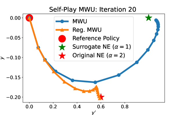
Figure 4: Motivating Example: 20 iterations of MWU and regularized MWU with the same learning rate to solve saddle point problem $\max_{y}\min_{y^{\prime}}f(y,y^{\prime},\alpha)$, where $f(y,y^{\prime};\alpha)=\frac{\alpha}{2}{y^{\prime}}^{2}+(y^{\prime}-1)(y-1)-\frac{\alpha}{2}y^{2}$, first introduced in [Sokota et al., 2022]. We assume that we only have access to a misspecified (surrogate) preference $f(y,y^{\prime};\alpha=1)$, while the ground truth human preference is $f(y,y^{\prime};\alpha=2)$.

The regularization in the preference model is not used in all game-theoretic self-play methods. Here we investigate the necessity of regularization and offer a motivating example in Figure 4, a saddle point solving problem $\min_{x}\max_{y}\frac{\alpha}{2}x^{2}+(x-1)(y-1)-\frac{\alpha}{2}y^{2}$. There exists a reference point as the initial values of $x$ and $y$. We assume that both reference point and the Nash Equilibrium (NE) of the surrogate preference model (Surrogate NE) are close to the original NE but on different sides of the original NE.

Typically, the surrogate preference/reward models are not positively related to the reference policy. Thus, it is a reasonable abstracted example of NLHF by treating the reference point as reference policy and surrogate NE as the optimal policy obtained by optimizing the surrogate preference/reward. The results of the $20$ iterations self-play MWU with an early stopping show that regularization can be used to prevent reward over-optimization (reaching surrogate NE). A well-tuned regularization leads to faster convergence to the unknown original NE. Thus, regularization can be effective in preventing over-optimization in self-play.

C.2 Diversity on 2D Example

We offer an analysis of our method compared to unregularized self-play (SPPO) on a 2D example in Figure 5. The area with a darker color is assigned a higher reward value. We use the preference defined by the $L^{2}$ norm between two actions. We also set the reference policy to be uniform. According to the figure, the unregularized method tends to converge to a single point on the manifold of the large reward. While regularized methods have diverse sampled actions.

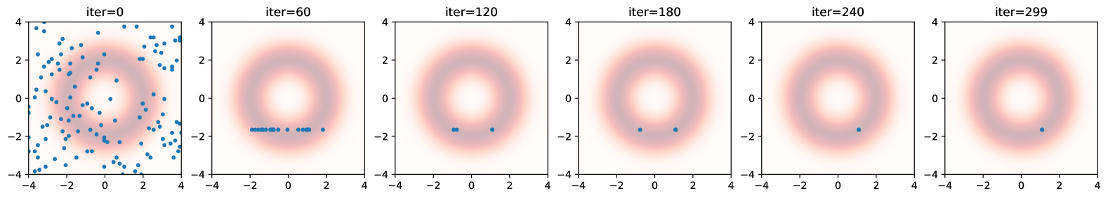
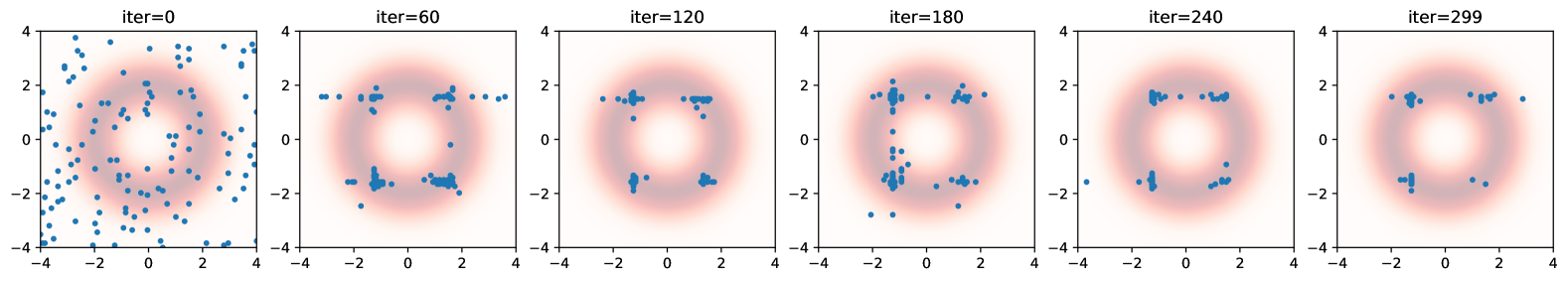
Figure 5: Samples in a 2D example of different iterations of SPPO (top) and RSPO (bottom) with external forward KL regularization to a uniform random reference policy. SPPO added simple external regularization that can generate multi-modal policies.

C.3 More Results on AlpacaEval-2.0

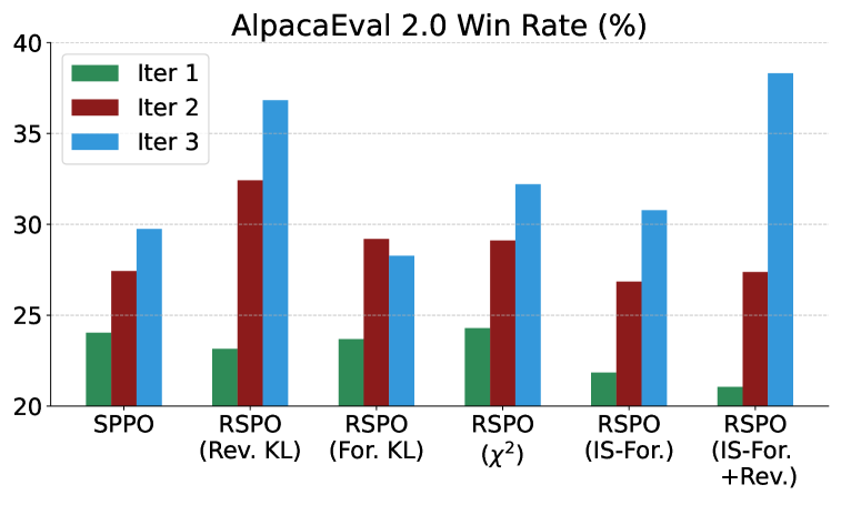
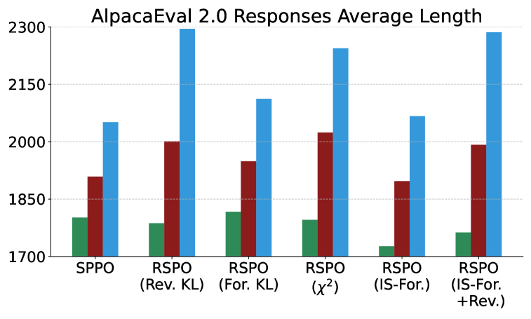
Figure 6: Win rates and the average length of SPPO and RSPO with different regularization methods. From left to right, regularization methods: Reverse KL, Forward KL, Chi-Squared, Importance-Sampling Forward KL, Importance-Sampling Forward, and Reverse KL linear combination.

References

- Meng et al. [2024] Yu Meng, Mengzhou Xia, and Danqi Chen. Simpo: Simple preference optimization with a reference-free reward. arXiv preprint arXiv:2405.14734, 2024.
- Wu et al. [2024] Yue Wu, Zhiqing Sun, Huizhuo Yuan, Kaixuan Ji, Yiming Yang, and Quanquan Gu. Self-play preference optimization for language model alignment. arXiv preprint arXiv:2405.00675, 2024.
- Jiang et al. [2023a] Albert Q Jiang, Alexandre Sablayrolles, Arthur Mensch, Chris Bamford, Devendra Singh Chaplot, Diego de las Casas, Florian Bressand, Gianna Lengyel, Guillaume Lample, Lucile Saulnier, et al. Mistral 7b. arXiv preprint arXiv:2310.06825, 2023a.
- Dubey et al. [2024] Abhimanyu Dubey, Abhinav Jauhri, Abhinav Pandey, Abhishek Kadian, Ahmad Al-Dahle, Aiesha Letman, Akhil Mathur, Alan Schelten, Amy Yang, Angela Fan, et al. The llama 3 herd of models. arXiv preprint arXiv:2407.21783, 2024.
- DeepSeek-AI et al. [2025] DeepSeek-AI, Daya Guo, Dejian Yang, Haowei Zhang, Junxiao Song, Ruoyu Zhang, Runxin Xu, Qihao Zhu, Shirong Ma, Peiyi Wang, Xiao Bi, Xiaokang Zhang, Xingkai Yu, Yu Wu, Z. F. Wu, Zhibin Gou, Zhihong Shao, Zhuoshu Li, Ziyi Gao, Aixin Liu, Bing Xue, Bingxuan Wang, Bochao Wu, Bei Feng, Chengda Lu, Chenggang Zhao, Chengqi Deng, Chenyu Zhang, Chong Ruan, Damai Dai, Deli Chen, Dongjie Ji, Erhang Li, Fangyun Lin, Fucong Dai, Fuli Luo, Guangbo Hao, Guanting Chen, Guowei Li, H. Zhang, Han Bao, Hanwei Xu, Haocheng Wang, Honghui Ding, Huajian Xin, Huazuo Gao, Hui Qu, Hui Li, Jianzhong Guo, Jiashi Li, Jiawei Wang, Jingchang Chen, Jingyang Yuan, Junjie Qiu, Junlong Li, J. L. Cai, Jiaqi Ni, Jian Liang, Jin Chen, Kai Dong, Kai Hu, Kaige Gao, Kang Guan, Kexin Huang, Kuai Yu, Lean Wang, Lecong Zhang, Liang Zhao, Litong Wang, Liyue Zhang, Lei Xu, Leyi Xia, Mingchuan Zhang, Minghua Zhang, Minghui Tang, Meng Li, Miaojun Wang, Mingming Li, Ning Tian, Panpan Huang, Peng Zhang, Qiancheng Wang, Qinyu Chen, Qiushi Du, Ruiqi Ge, Ruisong Zhang, Ruizhe Pan, Runji Wang, R. J. Chen, R. L. Jin, Ruyi Chen, Shanghao Lu, Shangyan Zhou, Shanhuang Chen, Shengfeng Ye, Shiyu Wang, Shuiping Yu, Shunfeng Zhou, Shuting Pan, S. S. Li, Shuang Zhou, Shaoqing Wu, Shengfeng Ye, Tao Yun, Tian Pei, Tianyu Sun, T. Wang, Wangding Zeng, Wanjia Zhao, Wen Liu, Wenfeng Liang, Wenjun Gao, Wenqin Yu, Wentao Zhang, W. L. Xiao, Wei An, Xiaodong Liu, Xiaohan Wang, Xiaokang Chen, Xiaotao Nie, Xin Cheng, Xin Liu, Xin Xie, Xingchao Liu, Xinyu Yang, Xinyuan Li, Xuecheng Su, Xuheng Lin, X. Q. Li, Xiangyue Jin, Xiaojin Shen, Xiaosha Chen, Xiaowen Sun, Xiaoxiang Wang, Xinnan Song, Xinyi Zhou, Xianzu Wang, Xinxia Shan, Y. K. Li, Y. Q. Wang, Y. X. Wei, Yang Zhang, Yanhong Xu, Yao Li, Yao Zhao, Yaofeng Sun, Yaohui Wang, Yi Yu, Yichao Zhang, Yifan Shi, Yiliang Xiong, Ying He, Yishi Piao, Yisong Wang, Yixuan Tan, Yiyang Ma, Yiyuan Liu, Yongqiang Guo, Yuan Ou, Yuduan Wang, Yue Gong, Yuheng Zou, Yujia He, Yunfan Xiong, Yuxiang Luo, Yuxiang You, Yuxuan Liu, Yuyang Zhou, Y. X. Zhu, Yanhong Xu, Yanping Huang, Yaohui Li, Yi Zheng, Yuchen Zhu, Yunxian Ma, Ying Tang, Yukun Zha, Yuting Yan, Z. Z. Ren, Zehui Ren, Zhangli Sha, Zhe Fu, Zhean Xu, Zhenda Xie, Zhengyan Zhang, Zhewen Hao, Zhicheng Ma, Zhigang Yan, Zhiyu Wu, Zihui Gu, Zijia Zhu, Zijun Liu, Zilin Li, Ziwei Xie, Ziyang Song, Zizheng Pan, Zhen Huang, Zhipeng Xu, Zhongyu Zhang, and Zhen Zhang. Deepseek-r1: Incentivizing reasoning capability in llms via reinforcement learning, 2025. URL https://arxiv.org/abs/2501.12948.
- Christiano et al. [2017] Paul F Christiano, Jan Leike, Tom Brown, Miljan Martic, Shane Legg, and Dario Amodei. Deep reinforcement learning from human preferences. Advances in neural information processing systems, 30, 2017.
- Ouyang et al. [2022] Long Ouyang, Jeffrey Wu, Xu Jiang, Diogo Almeida, Carroll Wainwright, Pamela Mishkin, Chong Zhang, Sandhini Agarwal, Katarina Slama, Alex Ray, et al. Training language models to follow instructions with human feedback. Advances in neural information processing systems, 35:27730–27744, 2022.
- Rafailov et al. [2024] Rafael Rafailov, Archit Sharma, Eric Mitchell, Christopher D Manning, Stefano Ermon, and Chelsea Finn. Direct preference optimization: Your language model is secretly a reward model. Advances in Neural Information Processing Systems, 36, 2024.
- Azar et al. [2024] Mohammad Gheshlaghi Azar, Zhaohan Daniel Guo, Bilal Piot, Remi Munos, Mark Rowland, Michal Valko, and Daniele Calandriello. A general theoretical paradigm to understand learning from human preferences. In International Conference on Artificial Intelligence and Statistics, pages 4447–4455. PMLR, 2024.
- Xiong et al. [2024] Wei Xiong, Hanze Dong, Chenlu Ye, Ziqi Wang, Han Zhong, Heng Ji, Nan Jiang, and Tong Zhang. Iterative preference learning from human feedback: Bridging theory and practice for rlhf under kl-constraint. In Forty-first International Conference on Machine Learning, 2024.
- Go et al. [2023] Dongyoung Go, Tomasz Korbak, Germán Kruszewski, Jos Rozen, Nahyeon Ryu, and Marc Dymetman. Aligning language models with preferences through f-divergence minimization. arXiv preprint arXiv:2302.08215, 2023.
- Huang et al. [2024] Audrey Huang, Wenhao Zhan, Tengyang Xie, Jason D Lee, Wen Sun, Akshay Krishnamurthy, and Dylan J Foster. Correcting the mythos of kl-regularization: Direct alignment without overoptimization via chi-squared preference optimization. arXiv preprint arXiv:2407.13399, 2024.
- Goodfellow et al. [2020] Ian Goodfellow, Jean Pouget-Abadie, Mehdi Mirza, Bing Xu, David Warde-Farley, Sherjil Ozair, Aaron Courville, and Yoshua Bengio. Generative adversarial networks. Communications of the ACM, 63(11):139–144, 2020.
- Wang et al. [2022] Zhendong Wang, Huangjie Zheng, Pengcheng He, Weizhu Chen, and Mingyuan Zhou. Diffusion-gan: Training gans with diffusion. arXiv preprint arXiv:2206.02262, 2022.
- Silver et al. [2016] David Silver, Aja Huang, Chris J Maddison, Arthur Guez, Laurent Sifre, George Van Den Driessche, Julian Schrittwieser, Ioannis Antonoglou, Veda Panneershelvam, Marc Lanctot, et al. Mastering the game of go with deep neural networks and tree search. nature, 529(7587):484–489, 2016.
- Heinrich and Silver [2016] Johannes Heinrich and David Silver. Deep reinforcement learning from self-play in imperfect-information games. arXiv preprint arXiv:1603.01121, 2016.
- Pinto et al. [2017] Lerrel Pinto, James Davidson, Rahul Sukthankar, and Abhinav Gupta. Robust adversarial reinforcement learning. In International conference on machine learning, pages 2817–2826. PMLR, 2017.
- Brown and Sandholm [2018] Noam Brown and Tuomas Sandholm. Superhuman ai for heads-up no-limit poker: Libratus beats top professionals. Science, 359(6374):418–424, 2018.
- Dubois et al. [2024] Yann Dubois, Balázs Galambosi, Percy Liang, and Tatsunori B Hashimoto. Length-controlled alpacaeval: A simple way to debias automatic evaluators. arXiv preprint arXiv:2404.04475, 2024.
- Jiang et al. [2024] Lingjie Jiang, Shaohan Huang, Xun Wu, and Furu Wei. Textual aesthetics in large language models. arXiv preprint arXiv:2411.02930, 2024.
- Rosset et al. [2024] Corby Rosset, Ching-An Cheng, Arindam Mitra, Michael Santacroce, Ahmed Awadallah, and Tengyang Xie. Direct nash optimization: Teaching language models to self-improve with general preferences. arXiv preprint arXiv:2404.03715, 2024.
- Munos et al. [2023] Rémi Munos, Michal Valko, Daniele Calandriello, Mohammad Gheshlaghi Azar, Mark Rowland, Zhaohan Daniel Guo, Yunhao Tang, Matthieu Geist, Thomas Mesnard, Andrea Michi, et al. Nash learning from human feedback. arXiv preprint arXiv:2312.00886, 2023.
- Calandriello et al. [2024] Daniele Calandriello, Daniel Guo, Remi Munos, Mark Rowland, Yunhao Tang, Bernardo Avila Pires, Pierre Harvey Richemond, Charline Le Lan, Michal Valko, Tianqi Liu, et al. Human alignment of large language models through online preference optimisation. arXiv preprint arXiv:2403.08635, 2024.
- David [1963] Herbert Aron David. The method of paired comparisons, volume 12. London, 1963.
- Swamy et al. [2024] Gokul Swamy, Christoph Dann, Rahul Kidambi, Zhiwei Steven Wu, and Alekh Agarwal. A minimaximalist approach to reinforcement learning from human feedback. arXiv preprint arXiv:2401.04056, 2024.
- Wang et al. [2024] Mingzhi Wang, Chengdong Ma, Qizhi Chen, Linjian Meng, Yang Han, Jiancong Xiao, Zhaowei Zhang, Jing Huo, Weijie J Su, and Yaodong Yang. Magnetic preference optimization: Achieving last-iterate convergence for language models alignment. arXiv preprint arXiv:2410.16714, 2024.
- Gao et al. [2024] Zhaolin Gao, Jonathan D Chang, Wenhao Zhan, Owen Oertell, Gokul Swamy, Kianté Brantley, Thorsten Joachims, J Andrew Bagnell, Jason D Lee, and Wen Sun. Rebel: Reinforcement learning via regressing relative rewards. arXiv preprint arXiv:2404.16767, 2024.
- Zhang et al. [2024] Yuheng Zhang, Dian Yu, Baolin Peng, Linfeng Song, Ye Tian, Mingyue Huo, Nan Jiang, Haitao Mi, and Dong Yu. Iterative nash policy optimization: Aligning llms with general preferences via no-regret learning, 2024. URL https://arxiv.org/abs/2407.00617.
- Beck and Teboulle [2003] Amir Beck and Marc Teboulle. Mirror descent and nonlinear projected subgradient methods for convex optimization. Operations Research Letters, 31(3):167–175, 2003.
- Pal et al. [2024] Arka Pal, Deep Karkhanis, Samuel Dooley, Manley Roberts, Siddartha Naidu, and Colin White. Smaug: Fixing failure modes of preference optimisation with dpo-positive. arXiv preprint arXiv:2402.13228, 2024.
- Schulman et al. [2017] John Schulman, Filip Wolski, Prafulla Dhariwal, Alec Radford, and Oleg Klimov. Proximal policy optimization algorithms. arXiv preprint arXiv:1707.06347, 2017.
- Bai et al. [2022] Yuntao Bai, Andy Jones, Kamal Ndousse, Amanda Askell, Anna Chen, Nova DasSarma, Dawn Drain, Stanislav Fort, Deep Ganguli, Tom Henighan, et al. Training a helpful and harmless assistant with reinforcement learning from human feedback. arXiv preprint arXiv:2204.05862, 2022.
- Touvron et al. [2023] Hugo Touvron, Louis Martin, Kevin Stone, Peter Albert, Amjad Almahairi, Yasmine Babaei, Nikolay Bashlykov, Soumya Batra, Prajjwal Bhargava, Shruti Bhosale, et al. Llama 2: Open foundation and fine-tuned chat models. arXiv preprint arXiv:2307.09288, 2023.
- Dong et al. [2024] Hanze Dong, Wei Xiong, Bo Pang, Haoxiang Wang, Han Zhao, Yingbo Zhou, Nan Jiang, Doyen Sahoo, Caiming Xiong, and Tong Zhang. Rlhf workflow: From reward modeling to online rlhf. arXiv preprint arXiv:2405.07863, 2024.
- Xu et al. [2023] Jing Xu, Andrew Lee, Sainbayar Sukhbaatar, and Jason Weston. Some things are more cringe than others: Preference optimization with the pairwise cringe loss. arXiv preprint arXiv:2312.16682, 2023.
- Liu et al. [2023] Tianqi Liu, Yao Zhao, Rishabh Joshi, Misha Khalman, Mohammad Saleh, Peter J Liu, and Jialu Liu. Statistical rejection sampling improves preference optimization. arXiv preprint arXiv:2309.06657, 2023.
- Tran et al. [2023] Hoang Tran, Chris Glaze, and Braden Hancock. Iterative dpo alignment. Technical report, Snorkel AI, 2023.
- Pang et al. [2024] Richard Yuanzhe Pang, Weizhe Yuan, Kyunghyun Cho, He He, Sainbayar Sukhbaatar, and Jason Weston. Iterative reasoning preference optimization. arXiv preprint arXiv:2404.19733, 2024.
- Guo et al. [2024] Shangmin Guo, Biao Zhang, Tianlin Liu, Tianqi Liu, Misha Khalman, Felipe Llinares, Alexandre Rame, Thomas Mesnard, Yao Zhao, Bilal Piot, et al. Direct language model alignment from online ai feedback. arXiv preprint arXiv:2402.04792, 2024.
- Tajwar et al. [2024] Fahim Tajwar, Anikait Singh, Archit Sharma, Rafael Rafailov, Jeff Schneider, Tengyang Xie, Stefano Ermon, Chelsea Finn, and Aviral Kumar. Preference fine-tuning of llms should leverage suboptimal, on-policy data. arXiv preprint arXiv:2404.14367, 2024.
- Cen et al. [2024] Shicong Cen, Jincheng Mei, Katayoon Goshvadi, Hanjun Dai, Tong Yang, Sherry Yang, Dale Schuurmans, Yuejie Chi, and Bo Dai. Value-incentivized preference optimization: A unified approach to online and offline rlhf. arXiv preprint arXiv:2405.19320, 2024.
- Xie et al. [2024] Tengyang Xie, Dylan J Foster, Akshay Krishnamurthy, Corby Rosset, Ahmed Awadallah, and Alexander Rakhlin. Exploratory preference optimization: Harnessing implicit q*-approximation for sample-efficient rlhf. arXiv preprint arXiv:2405.21046, 2024.
- Freund and Schapire [1997] Yoav Freund and Robert E Schapire. A decision-theoretic generalization of on-line learning and an application to boosting. Journal of computer and system sciences, 55(1):119–139, 1997.
- Jiang et al. [2023b] Dongfu Jiang, Xiang Ren, and Bill Yuchen Lin. Llm-blender: Ensembling large language models with pairwise comparison and generative fusion. In Proceedings of the 61th Annual Meeting of the Association for Computational Linguistics (ACL 2023), 2023b.
- Williams [1992] Ronald J Williams. Simple statistical gradient-following algorithms for connectionist reinforcement learning. Machine learning, 8:229–256, 1992.
- Tomar et al. [2020] Manan Tomar, Lior Shani, Yonathan Efroni, and Mohammad Ghavamzadeh. Mirror descent policy optimization. arXiv preprint arXiv:2005.09814, 2020.
- Haarnoja et al. [2018] Tuomas Haarnoja, Aurick Zhou, Pieter Abbeel, and Sergey Levine. Soft actor-critic: Off-policy maximum entropy deep reinforcement learning with a stochastic actor. In International conference on machine learning, pages 1861–1870. PMLR, 2018.
- Malkin et al. [2022] Nikolay Malkin, Salem Lahlou, Tristan Deleu, Xu Ji, Edward Hu, Katie Everett, Dinghuai Zhang, and Yoshua Bengio. Gflownets and variational inference. arXiv preprint arXiv:2210.00580, 2022.
- Sokota et al. [2022] Samuel Sokota, Ryan D’Orazio, J Zico Kolter, Nicolas Loizou, Marc Lanctot, Ioannis Mitliagkas, Noam Brown, and Christian Kroer. A unified approach to reinforcement learning, quantal response equilibria, and two-player zero-sum games. arXiv preprint arXiv:2206.05825, 2022.
- Bregman [1967] Lev M Bregman. The relaxation method of finding the common point of convex sets and its application to the solution of problems in convex programming. USSR computational mathematics and mathematical physics, 7(3):200–217, 1967.
- Sutton et al. [1999] Richard S Sutton, David McAllester, Satinder Singh, and Yishay Mansour. Policy gradient methods for reinforcement learning with function approximation. Advances in neural information processing systems, 12, 1999.
- Li et al. [2024] Tianle Li, Wei-Lin Chiang, Evan Frick, Lisa Dunlap, Tianhao Wu, Banghua Zhu, Joseph E Gonzalez, and Ion Stoica. From crowdsourced data to high-quality benchmarks: Arena-hard and benchbuilder pipeline. arXiv preprint arXiv:2406.11939, 2024.
- Zheng et al. [2023] Lianmin Zheng, Wei-Lin Chiang, Ying Sheng, Siyuan Zhuang, Zhanghao Wu, Yonghao Zhuang, Zi Lin, Zhuohan Li, Dacheng Li, Eric Xing, et al. Judging llm-as-a-judge with mt-bench and chatbot arena. Advances in Neural Information Processing Systems, 36:46595–46623, 2023.
- Cui et al. [2023] Ganqu Cui, Lifan Yuan, Ning Ding, Guanming Yao, Wei Zhu, Yuan Ni, Guotong Xie, Zhiyuan Liu, and Maosong Sun. Ultrafeedback: Boosting language models with high-quality feedback. 2023.
- Zhu et al. [2018] Yaoming Zhu, Sidi Lu, Lei Zheng, Jiaxian Guo, Weinan Zhang, Jun Wang, and Yong Yu. Texygen: A benchmarking platform for text generation models. In The 41st international ACM SIGIR conference on research & development in information retrieval, pages 1097–1100, 2018.
- Sion [1958] Maurice Sion. On general minimax theorems. 1958.
- Rubenstein et al. [2019] Paul Rubenstein, Olivier Bousquet, Josip Djolonga, Carlos Riquelme, and Ilya O Tolstikhin. Practical and consistent estimation of f-divergences. Advances in Neural Information Processing Systems, 32, 2019.