Genetics-Driven Personalized Disease Progression Model
Abstract.
Modeling disease progression through multiple stages is critical for clinical decision-making for chronic diseases, e.g., cancer, diabetes, chronic kidney diseases, and so on. Existing approaches often model the disease progression as a uniform trajectory pattern at the population level. However, chronic diseases are highly heterogeneous and often have multiple progression patterns depending on a patient’s individual genetics and environmental effects due to lifestyles. We propose a personalized disease progression model to jointly learn the heterogeneous progression patterns and groups of genetic profiles. In particular, an end-to-end pipeline is designed to simultaneously infer the characteristics of patients from genetic markers using a variational autoencoder and how it drives the disease progressions using an RNN-based state-space model based on clinical observations. Our proposed model shows improvement on real-world and synthetic clinical data.
1. Introduction
Chronic diseases such as Diabetes, Cancer and Huntington’s disease typically progress through multiple stages, ranging from mild to moderate to severe. A better understanding of progression of chronic diseases is crucial at multiple stages of clinical decision making such as early detection, preventive interventions, and precision medicine. Modeling the disease progression longitudinally from large scale patient records can also unravel important subtypes of the disease by representing its impact on sub-populations, from the rate of progression. Such disease progression models (DPM) have been used in clinical decision making for multiple chronic diseases such as Alzheimer’s disease (Sukkar et al., 2012; Liang et al., 2021; El-Sappagh et al., 2020), Huntington’s Disease (Sun et al., 2019; Mohan et al., 2022) and prostate cancer (Lee et al., 2022). Also, DPM has been used to assess the impact of novel therapeutics on the course of disease, thus elucidating a potential clinical benefit in the drug discovery process (Barrett et al., 2022; Goteti et al., 2023) and in designing clinical trials (Miller et al., 2005).
A few recent studies used deep learning based state-space models for DPMs, where multi-dimensional time-varying representations were used to learn disease states (Krishnan et al., 2017). For example, an attentive state-space model based on two recurrent neural networks (RNN) was used to remember the entire patients medical history from past electronic health records (EHR) which will ultimately govern transitions between states (Alaa and van der Schaar, 2019). Similarly, the representations of disease states were conditioned on patients treatment history to analyze the impact of diverse pharmaco-dynamic effects of multiple drugs (Hussain et al., 2021). In particular, they used multiple attention schemes, each modeling a pharmaco-dynamic mechanism of drugs, which ultimately determined the state representations of DPMs.
However, one caveat with these existing DPMs is their assumption that disease trajectory patterns are uniform across all patients as they progress through multiple stages. In reality, progression patterns differ widely from patient to patient due to their inherent genetic predisposition and environmental effects derived from to patient’s lifestyle (Dey et al., 2013). Previous approaches for disease progression pathways are often not personalized, rather they model disease progression as a uniform trajectory pattern at the population level. Although some recent proposed models, such as (Hussain et al., 2021), conditioned DPM on other available clinical observations including genetic data, demographics and treatment patterns, these models did not aim at building personalized DPMs based on patients genetic data.
In this work, our objective is to build a genetics-driven personalized disease progression model (PerDPM), where the progression model is built separately for each patient’s group associated with different inherent genetic makeups. The inherent characteristics of patients that drive the disease progression model differently are defined by their ancestry and inherent genetic composition. Specifically, we developed a joint learning framework, where the patient’s genetic grouping is discovered from large-scale genome-wide association studies (GWAS), along with developing disease progression models tailored to each identified genetic group. To achieve this, we first use a variational auto-encoder which identifies different groups of genetic clusters from GWAS data. Then, we model the disease progression model as a state-space model where the state transitions are dependent upon the genetic makeups, treatments and clinical history available so far. Our proposed model is generic enough to discover the genetic groupings and their associated progression pathway from clinical observations by utilizing both static (e.g., genetic data) and longitudinal healthcare records such as treatments, diagnostic variables measuring co-morbidities, and any clinical assessment of diseases such as laboratory measurements.
The main contributions of this paper can be summarized as below:
-
•
We proposed a genetic-driven disease personalized progression model (PerDPM). In PerDPM, we designed two novel modules: one for genetic makeups inference and another for genetics driven state transition modeling.
-
•
We introduced a joint learning optimization framework to infer both genetic makeups and latent disease states. This framework simultaneously performs clustering of genetic data and develops the genetic dependent disease progression model.
-
•
The proposed framework was tested both in synthetic and one of largest real-world EHR cohort collected from the UK called UKBioBank (UKBB). The effectiveness of the model was tested on this UKBB dataset in the context of modeling Chronic Kidney Disease.
2. Related Work
Disease progression models (DPM) provide a basis for learning from prior clinical experience and summarizing knowledge in a quantitative fashion. We refer to review article (Hainke et al., 2011) for general overview of DPM on multiple domains. The line of research for building DPM from longitudinal records belongs to the machine learning and artificial intelligence, where the state transitions are learned in a probabilistic manner. The earliest DPM technique was built upon Hidden Markov Models (Di Biase et al., 2007) to infer disease states and to estimate the transitional probabilities between them simultaneously. These baseline DPMs are mostly applicable for regular time intervals, while clinical observations are often collected at irregular intervals. A continuous-time progression model from discrete-time observations to learn the full progression trajectory has been proposed for this purpose (Wang et al., 2014; Bartolomeo et al., 2011). In (Liu et al., 2013) a 2D continuous-time Hidden Markov Model for glaucoma progression modeling from longitudinal structural and functional measurements is proposed. However, all of these probabilistic generative models are computationally expensive and not applicable for large-scale data analysis.
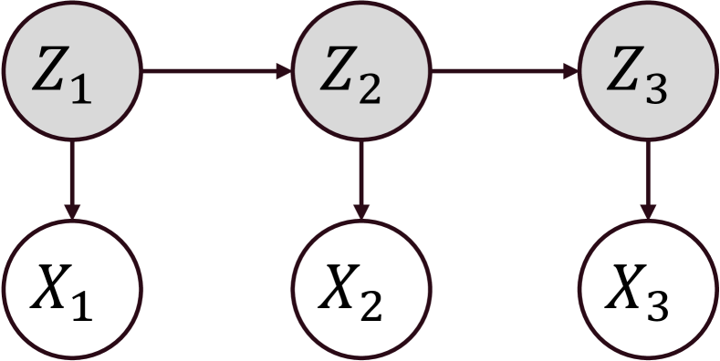
Recently, deep learning based generative Markov model such as state-space model (SSM) has been proposed for learning DPM from large-scale data. As shown in Fig. 1, the observational variables are generated from latent variables through emission models, and the transitions between latent variables correspond to the underlying dynamics of the system. Recent work added deep neural networks structure to linear Gaussian SSM to learn non-linear relationships from high dimensional time-series (Krishnan et al., 2017; Rangapuram et al., 2018; Ansari et al., 2021).
Interpretability has made SSM popular in modeling the progression of a variety of chronic diseases. For different diseases and different tasks, the design of SSM varies. In (Alaa and van der Schaar, 2019), a transition matrix in their model is used to learn interpretable state dynamics, as (Severson et al., 2020) introduces patient specific latent variables to learn personalized medication effects and (Hussain et al., 2021; Qian et al., 2021) focuses on pharmacodynamic model and integrating expert knowledge. To the best of our knowledge, none of these techniques is able to model how genetic heterogeneity may impact the disease progression directly through the integration of large-scale clinical and genomic data.
3. Notations
| Variables | Dimensions | Note |
| Temporal clinical features | ||
| Temporal treatments | ||
| Temporal latent states | ||
| Genetic features | ||
| Genetic group assignment matrix | ||
| Set of observable variables |
Let denote all the clinical features for a particular patient i, where , and represent the total number of clinical features and samples, respectively. Let denote the whole matrix of clinical observations from EHR. Also, EHR data are typically observed at multiple irregular time points. So, we use to denote the observed clinical features at time point t for the -th patient, where and denotes the total number of visits made by the patient . Through the paper, we will omit the sample index when there is no ambiguity. These clinical observations can consist of any temporal measurements such as prior disease history, lab assessments for the particular disease being model, image scans, etc. Let denote the final matrix of clinical observation containing all temporal data, where is the largest number of visits of patients. Similarly, denotes all treatments collected temporarily, where is the dimensions of all possible treatments performed on the patients. denotes genetic matrix, where is the total number of genetic features observed for patients. Note that genetics features are observed only during the initial visit of the patient, so genetic matrix don’t have any temporal dimensions associated with them. Further, we assume the whole population can be divided into different groups, expressing different disease progression dynamics and implicitly encoded by genetic information. In our model. we use a proxy variable to represent the probability of group assignment for each patient. Give patient’s clinical features , treatments , and genetic information , the final task is to learn latent representations , which describe the hidden states of the disease progression. For better understanding, we provide a lookup table for these notation in Table 1.
4. Method
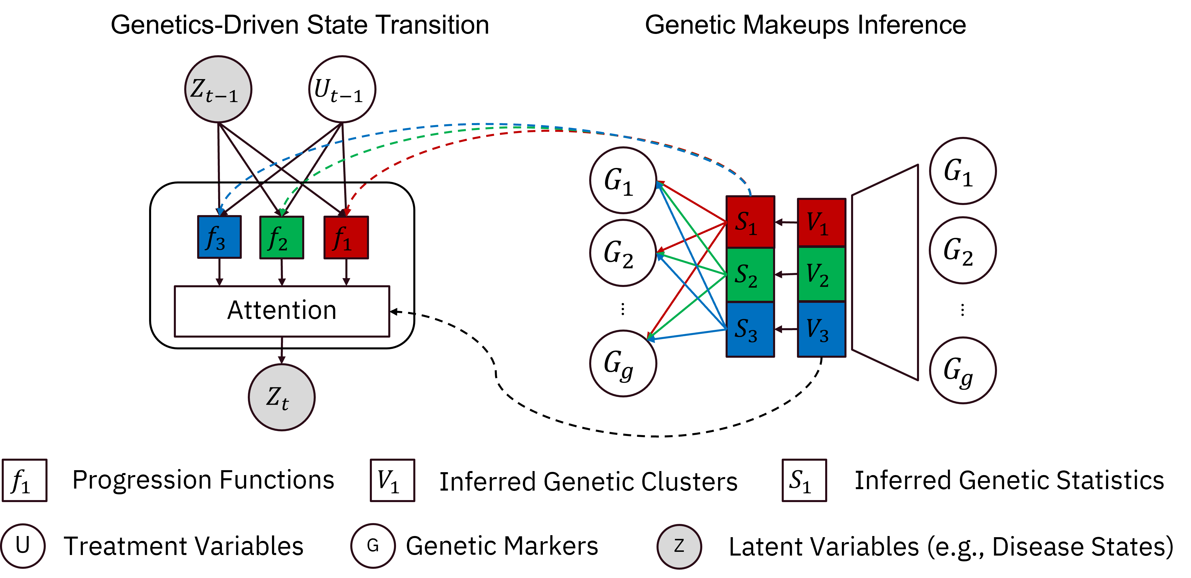
In this study, we want to extend the above mentioned state-space based disease progression models to a genetics driven personalized DPM model. Specifically, we want to make sure that the transitions between state s are conditioned on the genetic profile that is leaned from GWAS data as shown in Fig. 2. In addition to that, we also assume that the transition between states are dependent on the treatment patterns similar to (Hussain et al., 2021), so that the disease progression model can be better characterized by the genetics makeup of the patient.
Our proposed framework first models the genetic groupings from the available high-dimensional GWAS data using a variational auto-encoder, and then estimates the representations of disease progression through a generative framework with the above-mentioned assumptions of progression being conditioned on these genetic makeups and treatments.
In the rest of this section, we will first introduce our framework by factorizing the joint distribution of all observable variables according to previously mentioned methods. Then, we will derive the evidence lower bound (ELBO) for variational inference. Lastly, we will provide details on the generative model and the inference model for estimating genetic makeups and the disease states transitions.
4.1. Overall Framework
To characterize the disease progression using state-space models, a patient is modeled to be in a disease state at each time step , which is manifested in clinical observation . Specifically, in terms of observational data, we assume the clinical observations are generated from latent variables through an emission model. The disease progression from to is governed by a transition model and some observable variables such as treatments and genetic markers . Throughout the paper, we assume that the states are hidden and thus will be inferred in an unsupervised fashion.
We first model the joint distribution of all observable variables via the following factorization:
| (1) |
To further factorize the joint distribution , we introduce two latent variables: latent states and genetic cluster variable , to mimic the real data generation process. The variable describes the likelihood of a patient belonging to a certain genetic group. Then, term can be further factorized as follow:
| (2) | ||||
Here, the first equation follows our assumption that the joint distribution of and is conditioned the previous latent state and current treatment, which is the common assumption made by state space models. Then, in the second equation, we assumed the observations is conditionally-independent of genetic information given latent variables and treatment . Similarly, in the last equation, we assumed the observations is conditionally-independent of all other variables given latent state variables , the genetic information is conditionally-independent of all other variables given the latent proxy variable , and the latent proxy variable is independent of treatment
By combining Eq. 1 and Eq. 2, we obtain the joint probability of all the observable variables is
| (3) |
To make sure the edge case makes sense, we use a special setting for the initial latent state, i.e., .
4.2. Derivation of Evidence Lower Bound (ELBO)
Directly maximizing the likelihood shown in Section 4.1 is intractable. Instead, we learn via maximizing a variational lower bound (ELBO). For simplicity, let represents all observable variables, i.e., , and represent the dataset, the ELBO is
| (4) |
where and are learned posterior and prior distributions. Using Section 4.1 to expand Section 4.2 yields
We further factorize the ELBO into two components as follow:
| (5) |
As shown in the equation, we parameterized these two components using a VAE structure and state space models. The detailed derivation is given in the Supplementary section.
To minimize the ELBO, we follow the structural inference method proposed by (Krishnan et al., 2017). The key idea is to parameterize the inference models and generative models using differentiable neural network and update jointly using stochastic gradient descent. For the rest of this section, we introduce our design for inference models and generative models .
4.3. Genetic Makeups Inference
Typically, genetic data is collected in genome-wide association studies (GWAS), which measure the genetic variation of a person’s genome at a single base position. These variations, termed Single Nucleotide Polymorphisms (SNPs), impact how and to what degree a particular trait or disease phenotype is manifested in an individual. One particular challenge in modeling such genetic impact is the high-dimensionality and noise associated with GWAS data. Therefore, we deployed a generative model on the genetic data, assuming that there exist a few distinct genomic makeups for a particular disease, which manifest at different degrees in each individual sample.
To parameterize the inference models and generative models in the first two terms of Section 4.2, we propose a deep-learning algorithm based on a variational auto-encoder (VAE). For better interpretability and inference of latent states, we select a one-layer neural network as the VAE decoder. Specifically, the decoder is parameterized by a weight matrix , where is the number of genetic groups, and is the dimension of genetic features. Intuitively, the weight matrix decodes the distribution of genetic features for each cluster, and represents the assignments of each sample to a cluster . It’s important to note that we don’t require to be one-hot encoded in this context. The cluster assignment is done in a soft manner, allowing a single patient to be assigned to multiple clusters based on probability. The input of this module will be the genetic data . The clustering assignments and are learned jointly with the transition functions. More details are provided in Algorithm 1.
| (6) | ||||
| (7) |
4.4. Genetics Driven State Transition
In this subsetcion, we discuss how to design the genetics driven state transition, corresponding to and .
First, we use a GRU base inference network to capture the variational distribution of and sample the posterior. Specifically,
| (8) |
where is combiner function adding a skip connection to inference network, which is widely used in structural inference based methods (Krishnan et al., 2017; Alaa and van der Schaar, 2019; Hussain et al., 2021).
For , we designed a genetics-driven state transition module. Given the assumptions of progression being conditioned on these genetic makeups and treatments, we use a set of transition functions to model the genetics-driven disease progressions. To ensure that transition functions are conditioned on the genetic makeups, we associate each transition function with one genetic cluster as follows:
| (9) |
As shown in Eq. 9, each transition function takes the corresponding genetic makeups as input, together with previous latent state and treatment . We then use an attention mechanism to aggregate genetics-driven disease progressions. The weights of the attention are determined by the softmax of , which is jointly inferred with genetic makeups.
| (10) |
For the rest of the model, we used 2-layers neural networks with ReLU activation for generative model , i.e., . We provide additional details for the PerDPM model in Algorithm 1. The combiner function is presented in Algorithm 2.
4.5. Objective Function
Using aforementioned methods, the objective function can be written as follow following Section 4.2:
| (11) |
where
| (12) |
5. Experiment on Synthetic Dataset
5.1. Synthetic Dataset
A synthetic dataset is designed to simulate the progression of chronic disease, driven by genetic makeups. The generation process consists of the generation of genetic information, treatment, disease states and clinical observations.
5.1.1. Generation of Genetic Markers
As shown in Algorithm 3 lines 1-10, we first generated genetic markers for each patient as their inherent characteristics. Specifically, we first created genetic clusters and the corresponding genetic markers distributions . Then, a cluster assignment variable is created for each patient. The final genetic features were then derived by computing the average of the genetic marker distributions , with weights determined by the cluster assignment variables .
5.1.2. Generation of Treatments
To generate binary treatment variables, we randomly sample two time indices, and , indicating the start and ending points of treatments. Then, we set the corresponding entries to 1 in the treatment sequence, as shown in lines 11-14 in Algorithm 3.
5.1.3. Generation of Disease States
The disease states are latent variables describing the disease severity. The transition between different states depends,in reality, on multiple complex factors. In this synthetic dataset, we simplify the transitions model and make the disease progression driven by genetic markers. In lines 15-20 within Algorithm 3, we created a transition function for each genetic cluster . The state is computed by aggregating all transitions using the cluster assignment , followed by a softmax function. The initial disease states are sampled from a multivariate normal distribution, with individual-specific mean values (not genetic cluster-specific means).
5.1.4. Generation of Clinical Observations
The clinical observations are generated from the disease state through an emission model, parameterized by a linear model, as demonstrated in lines 22-23 in Algorithm 3.
5.2. Comparison Methods and Evaluation Metrics
We selected three state-of-the-art methods as comparison methods. All of these method are based on state space methods.
Deep Markov Models (DMM) (Krishnan et al., 2017): DNN is an algorithm designed to learn non-linear state space models. Following the structure of hidden Markov models (HMM), DMM employs multi-layer perceptrons (MLPs) to model the emission and transition distributions . The representational power of deep neural networks enables DMM to model high-dimensional data while preserving the Markovian properties of HMMs.
Attentive State-Space Model (ASSM) (Alaa and van der Schaar, 2019): ASSM learns discrete representations for disease trajectories. ASSM introduces the attention mechanism to learn the dependence of future disease states on past medical history. In ASSM, state transitions are approximated by a weighted average of the transition probability from all previous states. i.e., , where is a learnable attention weight, and is the predefined transition matrix obtained from observations using a Gaussian Mixture model.
Intervention Effect Functions (IEF) (Hussain et al., 2021): IEF-based disease progression model is a deep state space model designed for learning the effect of drug combinations, i.e., pharmacodynamic. IEF proposes an attention based neural network architecture to learn the pharmacodynamic, i.e., how treatments affect disease states. Although IEF is not tailored for genetics-driven progression models, it has the capacity of incorporating individual-specific covariates. Thus, in the experiments, we test two variants of IEF: one without using genetic information (named IEF) and one using genetic information as static covariates (named IEF w/ G).
For the evaluation metrics, we report the test negative log likelihood (NLL) of clinical observations on synthetic dataset. In the real-world dataset, the clinical observations are binary variables, and we reported the Cross-Entropy (CE) instead. We also reported the Pearson’s chi-square statistic (Chi2) between the predicted states and the true states, calculated using a contingency table. The Chi2 score measure the discrepancies between the predicted results and the expected frequencies, which can be seen as the random guess in our case. Thus, a higher Chi2 score is better. For both NLL and CE score, lower values are better.
5.3. Results on Synthetic Dataset
Utilizing the data generation method introduced in Section 5.1, we created 5 different datasets using with various settings. The number of disease states and the number of genetic clusters are both set to 5 for all these five datasets. For each dataset, we performed 10 random train-test splits and conducted evaluations using comparison methods. The results for the synthetic dataset 1 are reported in Table 2 (10 experiments). Additionally, we report the results for all the synthetic dataset in Table 4 (50 experiments) in the Appendix. It’s worth noting that the comparison method ASSM does not maximize the likelihood of clinical observations directly and doesn’t provide the estimated mean and variance for the covariates. Therefore, we didn’t report the negative log likelihood (NLL) for ASSM.
As shown in Table 2, DMM shows the worst performance compared to all other methods. Similar to a hidden Markov model, DMM assumes that all patients follow the same transition pattern, as the transitions between latent states are modeled by the same neural networks. When the latent dynamic of state transition varies according to patient’s inherited characters, the assumption of DMM fails. Modeling the transition uniformly prohibits DMM to capture genetic driven disease progression in our synthetic dataset.
Compared to DMM, ASSM and IEF incorporate attention mechanisms into their transition models, enabling them to capture the variations in transition patterns. In Table 2, ASSM and IEF show better scores than DMM in both NLL and Chi2. Considering the similarity in the generative models of IEF and DMM, the lower NLL for IEF suggests it learned a better representation of latent states by using attention mechanisms. Also, higher Chi2 scores suggest the inferred latent states from IEF and ASSM are closer to the true states than those inferred from DMM.
When incorporating genetic information, the IEF w/ G can be seen as the personalized model. The difference in performance between IEF w/ G and IEF indicates that using genetic information is helpful for personalized disease modeling. However, the performance gaps between IEF w/G and IEF become smaller as the training set size decreases. This suggests that the simple concatenation of genetic information and clinical observation is insufficient to learn the genetic clusters and the disease progression pattern it drives, especially in the case when the genetic information is noisy.
| Methods | ASSM | DMM | IEF | IEF w/ G | PerDPM | Trainin Set Size |
| NLL | 600 | |||||
| Chi2 | ||||||
| NLL | 1500 | |||||
| Chi2 | ||||||
| NLL | 3000 | |||||
| Chi2 |
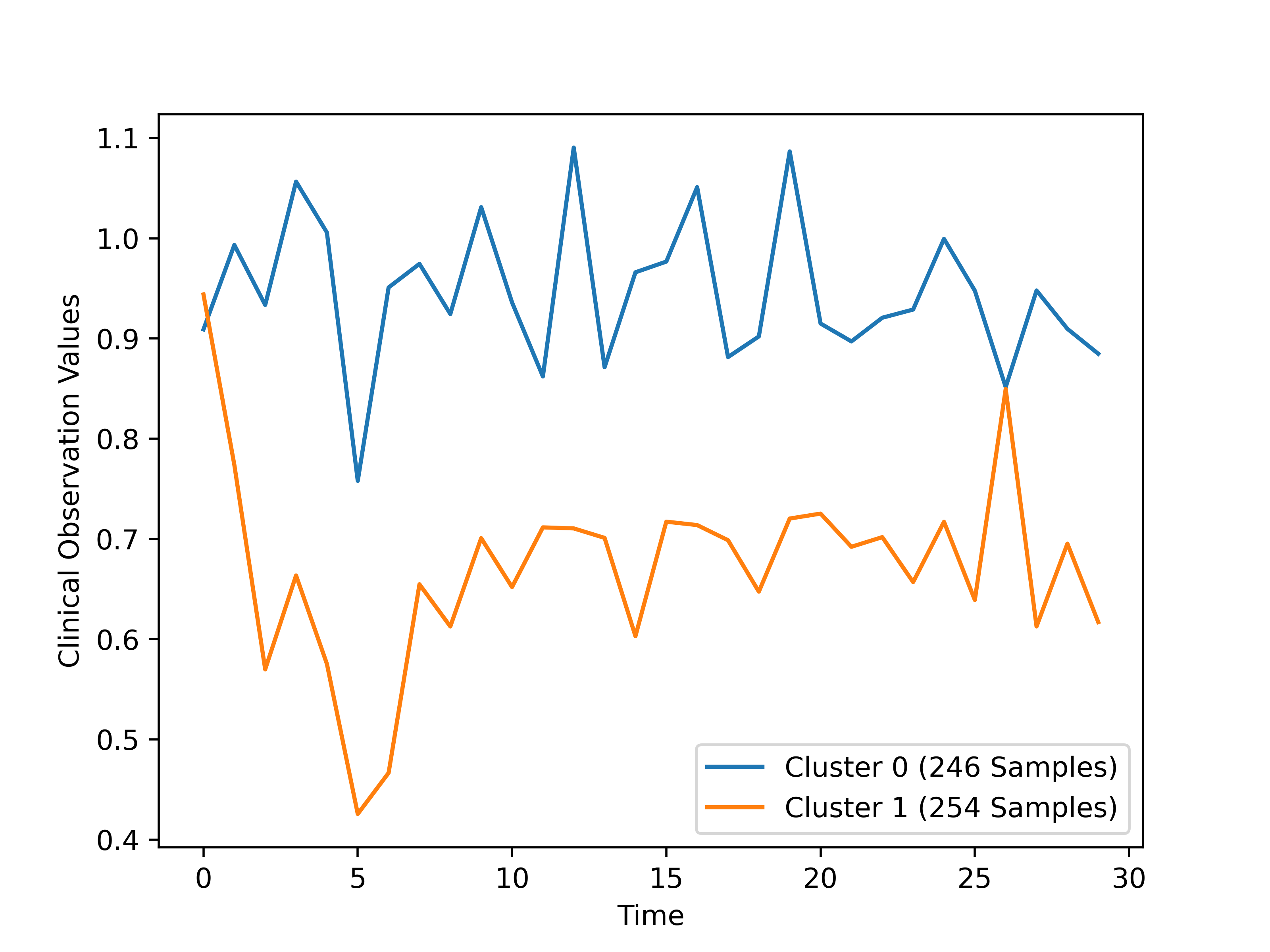
Our model outperforms all other methods in both metrics, and the improvement becomes more significant as the sample size increase. To further assess the effectiveness of our model, we conducted additional analysis on the discovered genetic groups to assess how well they can segregate the disease progression patterns. We used KMeans to learn two genetic clusters using the representations of the inferred clusters variables . Then, we plotted the mean values of one dimension of observation, i.e., , along the timeline for each cluster in Fig. 3. Clearly, samples from these two clusters have very different observation values, although these two clusters have similar initial values. This demonstrates that our designed genetics-driven state transition can effectively identify different transition patterns governed by diverse genetic makeups for different genetics clusters.
6. Results on modeling progression of Chronic Kidney Disease
6.1. Real-World Chronic Kidney Disease Dataset
Chronic kidney disease (CKD) is a condition where the kidneys are damaged and progressively lose their ability to filter blood. It is estimated that millions or of the world population have CKD (Kovesdy, 2022) and millions in the USA alone, it being one of the leading causes of death while of adults with CKD and of adults with severe CKD do not know that they already have the disease (for Disease Control and Prevention, 2021). CKD is primarily defined in Clinical Practice Guidelines in terms of kidney function (National Kidney Foundation, 2002) and CKD patients progress over five CKD stages, often slowly and heterogenously (Abeysekera et al., 2021), from mild kidney damage to End Stage Kidney Disease (ESKD) or kidney failure, defined as either the initiation of dialysis or kidney transplant. Later stages of CKD are defined based on lower levels of creatinine-based estimated glomerular filtration rate (eGFR below ml min m-2) hence capturing an heterogeneous set of kidney disorders. However, eGFR has been used in a set of genomic studies as a trait for finding common variants associated with kidney disease. GWAS can explain up to of an estimated heritability in this CKD-associated trait (Wuttke et al., 2019) and have helped establish genome-wide polygenic scores (GPS) across ancestries for discriminating moderate-to-advanced CKD from population controls (Khan et al., 2022).
We used a large-scale real world dataset containing approximately 250,000 samples from the UK, collected as UKBioBank repository (Sudlow et al., 2015) to validate our proposed GWA-PerDPM model. We extracted clinical features such as clinical classification system (CCS) codes for measuring co-morbidities and therapeutic drug classes for measuring the treatments in the context of modeling chronic kidney disease (CKD). We also curated approximately 300 SNPs from the genome-wide-association (GWA) using the common quality control protocols. Furthermore, we computed the true stages of CKD based on the eGFR measurements that were available in the dataset.
6.2. Result of Chronic Kidney Disease Progression Modeling
We reported the results on real-world chronic kidney disease dataset in Table 3. In our CKD dataset, clinical observations consist of binary CCS codes, which makes ASSM infeasible for use since it employs conditional density estimation. Therefore, In this section, we only compare our proposed method with IEF since it is easy to modify to handle binary clinical observations. In both IEF and our method, we adjusted the ELBO by adopting cross entropy to accommodate the binary nature of the clinical observations, and we reported cross entropy (CE) instead of negative log-likelihood (NLL) in the table to measure how well the generative models fit the observations.
As shown in Table 3, the results are consistent with those obtained from the synthetic dataset, demonstrating that our methods outperform other methods in both metrics. it’s worth nothing that the score gap between PerDPM and IEF w/ G becomes larger in the CKD progression modeling. One reason could be the increased noise in clinical observations (we use the binary diagnosis code as clinical observation). Also, genetic information shows less correlation with disease progression, considering the fact that GWAS can only explain up to 20% of an estimated 54% heritability in this CKD-associated trait. This emphasizes the necessity of modeling genetic driven dynamic explicitly.
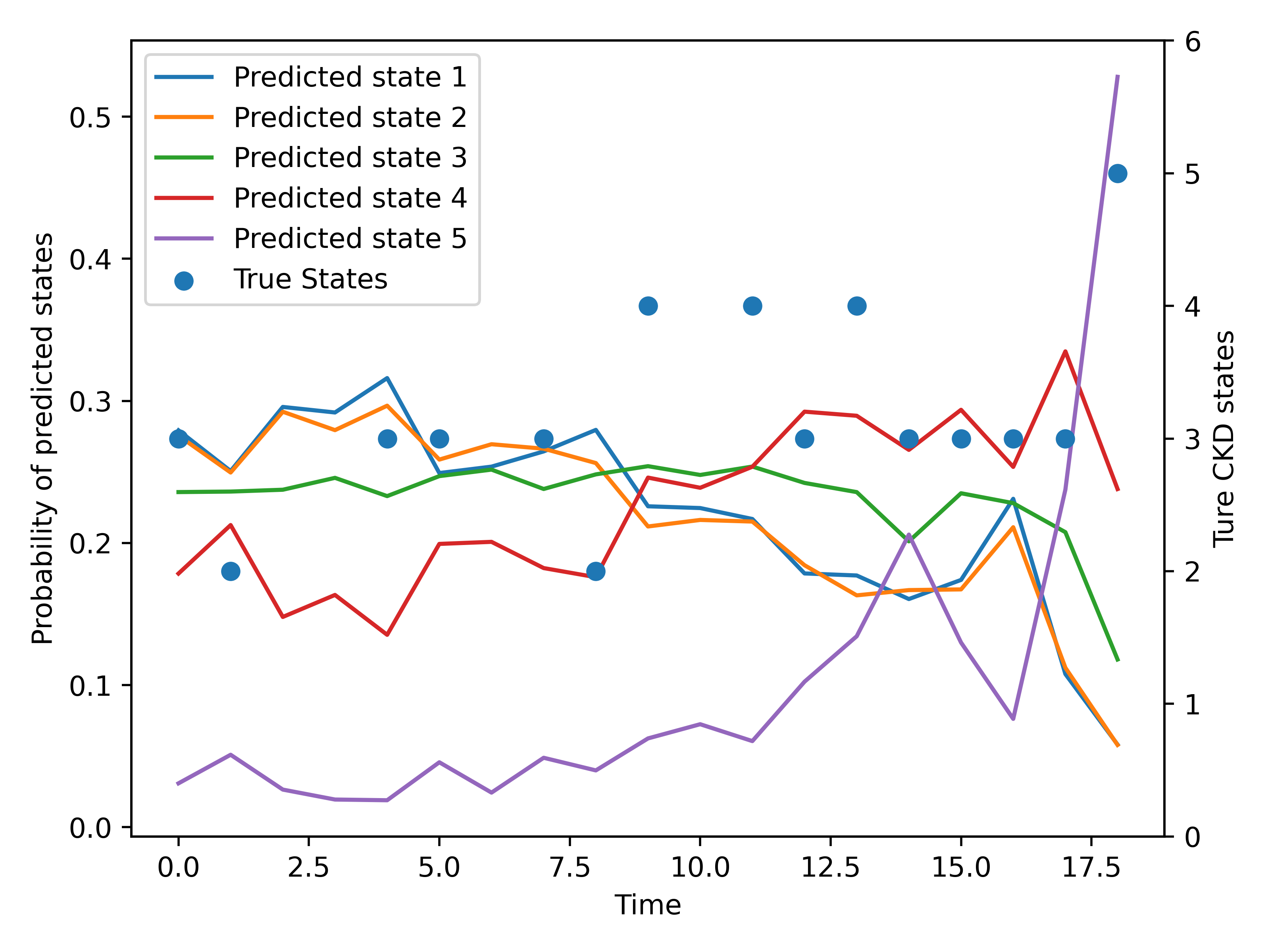
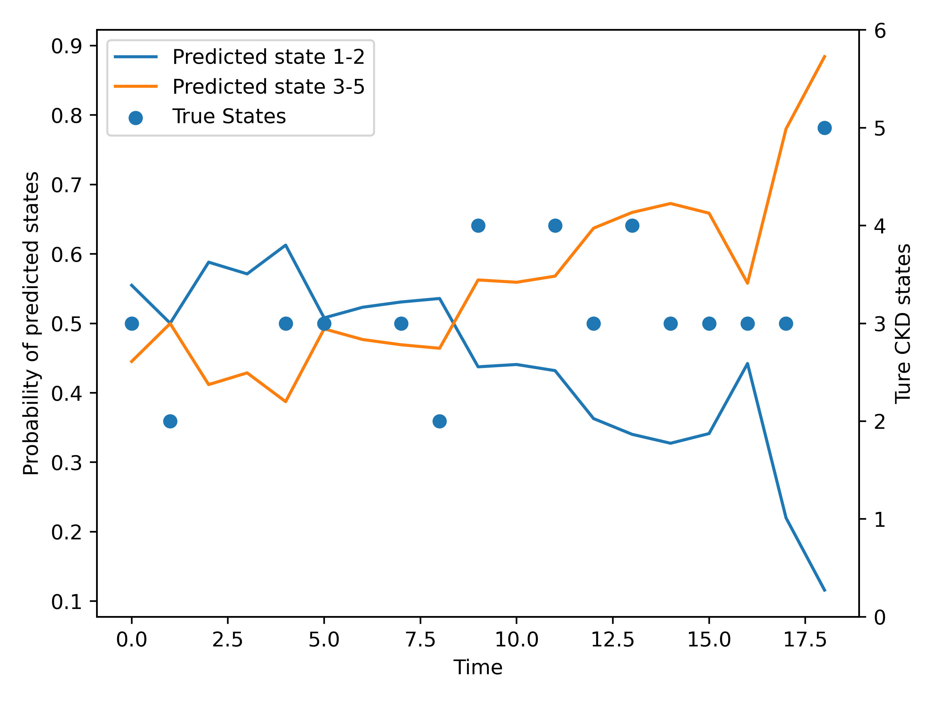
In Fig. 4, we visualized the inferred hidden states from our method for one patient, along with the true CKD states. In the figure, we plot the probability of each inferred state as color-coded lines, with the corresponding values plotted on the left-hand side of the y-axis. For example, at time 0, the predicted probability of the patient being in CKD state 2 is about 0.28 since the orange line has value 0.28 at . The true CKD states are represented by the blue dots at the date when the eGFR is measured, which is the indicator of CKD severity. These CKD states vary among , reflecting the degrees of severity, with corresponding discrete state values shown on the right-hand side of the y-axis. For example, the patient was diagnosed with CKD stage 3 at time 0, as the first blue dot reads number 3 on the right-hand side of the y-axis. As shown in Fig. 4, as the disease progress, the probability of predicted state 1, 2, and 3 gradually decrease, while the probabilities of predicted state 4, 5 gradually increase. The dynamic of the inferred states is consistent with the patient’s true CKD progression. If we choose the inferred state based on the highest predicted probability, the inferred states align well with the true states represented by the blue dots.
In chronic kidney disease, CKD stage 1 and 2 correspond to mild conditions. People are usually considered as not having CKD in the absence of markers of kidney damage when they are in state 1 and 2. Following this criterion and for better visualization, we further aggregate the probability of states 1 and 2, as well as the probability of states 3-5 from our model, to binarize the predicted progression into CKD and no CKD. The visualization is shown in Fig. 5. The probability of predicted states also aligns well with the true states represented by the blue dots.
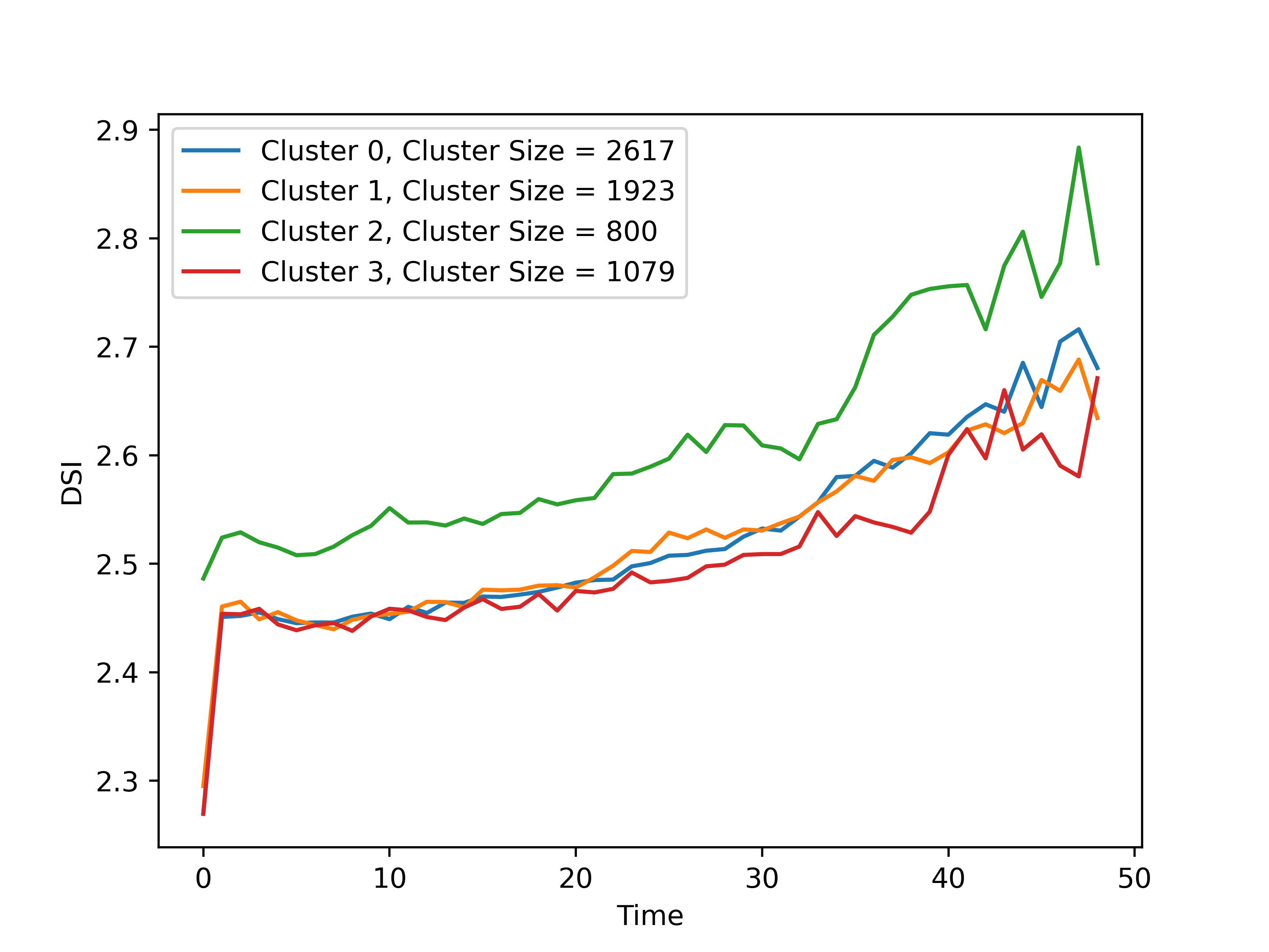
To further analyse if the proposed model learned genetics driven progression, we plot the disease severity index (DSI) per each time steps for each genetic group in Fig. 6. DSI is defined as the expected disease states by the following equation: , for -th sample and -th time point and each possible discrete states . In Fig. 6, each line shows the change in mean DSI as disease progress in each genetic cluster. As shown in the figure, genetic cluster 2 exhibits different behavior than the other three clusters. Patients in cluster group 2 have higher CKD risk at their index day (first visit) and are more likely to progress into more severe stages. On the other hand, all other clusters started at same DSI, but patients in cluster 3 tend to have a lower DSI at later stages. This shows the presence of genetic impacts on the progression patterns in CKD and the ability of our model to capture them.
| Methods | IEF | IEF w/ G | PerDPM |
| CE | |||
| Chi2 |
7. Conclusion
In this paper, we developed a personalized disease progression model based on the heterogeneous genetic makeups, clinical observations, and treatments of individual patients. We jointly inferred the latent disease states and genetics-driven disease progressions using the proposed genetic makeups inference module and genetics-driven state transition module. We demonstrated improvements over state-of-the-art methods using both synthetic data and a large-scale real-world dataset from the UK BioBank cohort of Chronic Kidney Disease. Our analysis shows that the proposed model is generic enough to discover diverse genetic profiles and associated disease progression patterns. Therefore, it can be deployed in the future on a wide variety of healthcare datasets for deriving useful clinical insights.
References
- (1)
- ome (2017) 13 Oct, 2017. https://www.webmd.com/drugs/2/drug-3766-2250/omeprazole-oral/omeprazole-delayed-release-tablet-oral/details/list-sideeffects. (13 Oct, 2017).
- ICD (2015) 2015. ICD9 Codes. https://www.cdc.gov/nchs/icd/icd9.htm.
- RB (2015) 2015. Redbook. http://micromedex.com/products/product-suites/clinical-knowledge/redbook.
- Abeysekera et al. (2021) Rajitha A Abeysekera, Helen G Healy, Zaimin Wang, Anne L Cameron, and Wendy E Hoy. 2021. Heterogeneity in patterns of progression of chronic kidney disease. Internal medicine journal 51, 2 (2021), 220–228.
- Alaa and van der Schaar (2019) Ahmed M Alaa and Mihaela van der Schaar. 2019. Attentive state-space modeling of disease progression. Advances in neural information processing systems 32 (2019).
- Alyass et al. (2015) Akram Alyass, Michelle Turcotte, and David Meyre. 2015. From big data analysis to personalized medicine for all: challenges and opportunities. BMC Medical Genomics 8, 33 (2015).
- Ansari et al. (2021) Abdul Fatir Ansari, Konstantinos Benidis, Richard Kurle, Ali Caner Turkmen, Harold Soh, Alexander J Smola, Bernie Wang, and Tim Januschowski. 2021. Deep explicit duration switching models for time series. Advances in Neural Information Processing Systems 34 (2021), 29949–29961.
- Barrett et al. (2022) Jeffrey S Barrett, Tim Nicholas, Karim Azer, and Brian W Corrigan. 2022. Role of disease progression models in drug development. Pharmaceutical Research 39, 8 (2022), 1803–1815.
- Bartolomeo et al. (2011) Nicola Bartolomeo, Paolo Trerotoli, and Gabriella Serio. 2011. Progression of liver cirrhosis to HCC: an application of hidden Markov model. BMC Medical Research Methodology 11, 1 (2011), 38.
- Bilen et al. (2016) Ozlem Bilen, Ayeesha Kamal, and Salim S Virani. 2016. Lipoprotein abnormalities in South Asians and its association with cardiovascular disease: Current state and future directions. World journal of cardiology 8, 3 (2016), 247.
- Boyd et al. (2005) Cynthia Boyd, Jonathan Darer, Chad Boult, et al. 2005. Clinical practice guidelines and quality of care for older patients with multiple comorbid diseases: implications for pay for performance. The Journal of the American Medical Association (JAMA) 294, 6 (2005), 716–724.
- Boyd et al. (2011) Stephen Boyd, Neal Parikh, Eric Chu, et al. 2011. Distributed optimization and statistical learning via the alternating direction method of multipliers. Foundations and Trends in Machine Learning 3, 1 (2011), 1122.
- Brown et al. (2018) Adam S Brown, Danielle Rasooly, and Chirag J Patel. 2018. Leveraging Population-Based Clinical Quantitative Phenotyping for Drug Repositioning. CPT: pharmacometrics & systems pharmacology 7, 2 (2018), 124–129.
- Cao et al. (2015) D-S Cao, N Xiao, Y-J Li, et al. 2015. Integrating multiple evidence sources to predict adverse drug reactions based on a systems pharmacology model. CPT: pharmacometrics & systems pharmacology 4, 9 (2015), 498–506.
- Ceriello et al. (2014) Antonio Ceriello, Marco Gallo, Riccardo Candido, Alberto De Micheli, Katherine Esposito, Sandro Gentile, and Gerardo Medea. 2014. Personalized therapy algorithms for type 2 diabetes: a phenotype-based approach. Pharmacogenomics and Personalized Medicine 7 (2014), 129–136.
- Chen and Snyder (2012) Rui Chen and Michael Snyder. 2012. Promise of personalized omics to precision medicine. Wiley Interdisciplinary Reviews: Systems Biology and Medicine 5, 1 (2012), 73–82.
- Cheng and Church (2000) Yizong Cheng and George M Church. 2000. Biclustering of expression data.. In Ismb, Vol. 8. 93–103.
- Cormen et al. (2009) Thomas H Cormen, Charles E Leiserson, Ronald L Rivest, and Clifford Stein. 2009. Introduction to algorithms. MIT press.
- Dannemann and Holzmann (2008) J Dannemann and H Holzmann. 2008. Likelihood Ratio Testing for Hidden Markov Models Under Non-standard Conditions. Scandinavian Journal of Statistics 35, 2 (2008), 309–321.
- Dey et al. (2013) Sanjoy Dey, Rohit Gupta, Michael Steinbach, and Vipin Kumar. 2013. Integration of clinical and genomic data: a methodological survey. (2013).
- Di Biase et al. (2007) Giuseppe Di Biase, Guglielmo D’Amico, Arturo Di Girolamo, Jacques Janssen, Stefano Iacobelli, Nicola Tinari, and Raimondo Manca. 2007. A stochastic model for the HIV/AIDS dynamic evolution. Mathematical Problems in Engineering 2007 (2007).
- El-Sappagh et al. (2020) Shaker El-Sappagh, Tamer Abuhmed, SM Riazul Islam, and Kyung Sup Kwak. 2020. Multimodal multitask deep learning model for Alzheimer’s disease progression detection based on time series data. Neurocomputing 412 (2020), 197–215.
- FDA (2016) FDA. 2016. FDA’s Adverse Event Reporting System (FAERS). https://www.fda.gov/Drugs/GuidanceComplianceRegulatoryInformation/Surveillance/AdverseDrugEffects/
- Fernald et al. (2011) Guy Fernald, Emidio Capriotti, Roxana Daneshjou, Konrad Karczewski, and Russ Altman. 2011. Bioinformatics challenges for personalized medicine. Bioinformatics 27, 13 (2011), 1741–1748.
- for Disease Control and Prevention (2021) Centers for Disease Control and Prevention. 2021. Chronic Kidney Disease in the United States. US Department of Health and Human Services, Centers for Disease Control and Prevention (2021).
- Ghalwash et al. (2017) Mohamed Ghalwash, Ying Li, Ping Zhang, and Jianying Hu. 2017. Exploiting electronic health records to mine drug effects on laboratory test results. In ACM on Conference on Information and Knowledge Management. 1837–1846.
- Goteti et al. (2023) Kosalaram Goteti, Nathan Hanan, Mindy Magee, Jessica Wojciechowski, Sven Mensing, Bojan Lalovic, Yaming Hang, Alexander Solms, Indrajeet Singh, Rajendra Singh, et al. 2023. Opportunities and Challenges of Disease Progression Modeling in Drug Development–An IQ Perspective. Clinical Pharmacology & Therapeutics (2023).
- Gottlieb et al. (2013) Assaf Gottlieb, Gideon Stein, Eytan Ruppin, Russ Altman, and Roded Sharan. 2013. A method for inferring medical diagnoses from patient similarities. BMC Medicine 11 (2013), 194.
- Gottlieb et al. (2011) Assaf Gottlieb, Gideon Y Stein, Eytan Ruppin, and Roded Sharan. 2011. PREDICT: a method for inferring novel drug indications with application to personalized medicine. Molecular systems biology 7, 1 (2011), 496.
- Hahr and Molitch (2015) Allison Hahr and Mark Molitch. 2015. Management of diabetes mellitus in patients with chronic kidney disease. Clinical Diabetes and Endocrinology 1, 2 (2015).
- Hainke et al. (2011) Katrin Hainke, Jörg Rahnenführer, and Roland Fried. 2011. Disease progression models: A review and comparison. Dortmund University, Technical Report (2011).
- Harpaz et al. (2013) Rave Harpaz, William DuMouchel, Paea LePendu, et al. 2013. Performance of Pharmacovigilance Signal-Detection Algorithms for the FDA Adverse Event Reporting System. Clinical Pharmacology & Therapeutics 93, 6 (2013), 539–546.
- Hussain et al. (2021) Zeshan M Hussain, Rahul G Krishnan, and David Sontag. 2021. Neural pharmacodynamic state space modeling. In International Conference on Machine Learning. PMLR, 4500–4510.
- Keiser et al. (2009) Michael J Keiser, Vincent Setola, John J Irwin, et al. 2009. Predicting new molecular targets for known drugs. Nature 462, 7270 (2009), 175.
- Khan et al. (2022) Atlas Khan, Michael C Turchin, Amit Patki, Vinodh Srinivasasainagendra, Ning Shang, Rajiv Nadukuru, Alana C Jones, Edyta Malolepsza, Ozan Dikilitas, Iftikhar J Kullo, et al. 2022. Genome-wide polygenic score to predict chronic kidney disease across ancestries. Nature Medicine 28, 7 (2022), 1412–1420.
- Kong et al. (2014) Deguang Kong, Ryohei Fujimaki, Ji Liu, Feiping Nie, and Chris Ding. 2014. Exclusive Feature Learning on Arbitrary Structures via -norm. In Advances in Neural Information Processing Systems. 1655–1663.
- Kovesdy (2022) Csaba P Kovesdy. 2022. Epidemiology of chronic kidney disease: an update 2022. Kidney International Supplements 12, 1 (2022), 7–11.
- Kowalski (2009) Matthieu Kowalski. 2009. Sparse regression using mixed norms. Applied and Computational Harmonic Analysis 27, 3 (2009), 303–324.
- Krishnan et al. (2017) Rahul Krishnan, Uri Shalit, and David Sontag. 2017. Structured inference networks for nonlinear state space models. In Proceedings of the AAAI Conference on Artificial Intelligence, Vol. 31.
- Kuang et al. (2014) Qifan Kuang, MinQi Wang, Rong Li, et al. 2014. A systematic investigation of computation models for predicting adverse drug reactions (ADRs). PloS one 9, 9 (2014), e105889.
- Kuang et al. (2016a) Zhaobin Kuang, James Thomson, Michael Caldwell, et al. 2016a. Baseline regularization for computational drug repositioning with longitudinal observational data. In IJCAI: proceedings of the conference, Vol. 2016. NIH Public Access, 2521.
- Kuang et al. (2016b) Zhaobin Kuang, James Thomson, Michael Caldwell, et al. 2016b. Computational drug repositioning using continuous self-controlled case series. In KDD: proceedings. International Conference on Knowledge Discovery Data Mining, Vol. 2016. NIH Public Access, 491.
- Kuhn et al. (2015) Michael Kuhn, Ivica Letunic, Lars Jensen, and Peer Bork. 2015. The SIDER database of drugs and side effects. Nucleic Acids Research 44, D1 (2015), D1075–D1079.
- Lasagna (2000) Louis Lasagna. 2000. Diuretics vs alpha-blockers for treatment of hypertension: lessons from ALLHAT. The Journal of the American Medical Association (JAMA) 283, 15 (2000).
- Lee et al. (2022) Changhee Lee, Alexander Light, Evgeny S Saveliev, Mihaela Van der Schaar, and Vincent J Gnanapragasam. 2022. Developing machine learning algorithms for dynamic estimation of progression during active surveillance for prostate cancer. npj Digital Medicine 5, 1 (2022), 110.
- Liang et al. (2021) Wei Liang, Kai Zhang, Peng Cao, Xiaoli Liu, Jinzhu Yang, and Osmar Zaiane. 2021. Rethinking modeling Alzheimer’s disease progression from a multi-task learning perspective with deep recurrent neural network. Computers in Biology and Medicine 138 (2021), 104935.
- Liu et al. (2013) Yu-Ying Liu, Hiroshi Ishikawa, Mei Chen, Gadi Wollstein, Joel S Schuman, and James M Rehg. 2013. Longitudinal modeling of glaucoma progression using 2-dimensional continuous-time hidden markov model. In Medical Image Computing and Computer-Assisted Intervention–MICCAI 2013: 16th International Conference, Nagoya, Japan, September 22-26, 2013, Proceedings, Part II 16. Springer, 444–451.
- Luo et al. (2016) Heng Luo, Ping Zhang, Xi Hang Cao, et al. 2016. Dpdr-cpi, a server that predicts drug positioning and drug repositioning via chemical-protein interactome. Scientific reports 6 (2016), 35996.
- MacDonald et al. (2010) Michael MacDonald, Dean Eurich, Sumit Majumdar, et al. 2010. Treatment of type 2 diabetes and outcomes in patients with heart failure: a nested case control study from the UK general practice research database. Diabetes Care 33, 6 (2010), 1213–1218.
- Madeira and Oliveira (2004) Sara C Madeira and Arlindo L Oliveira. 2004. Biclustering algorithms for biological data analysis: a survey. IEEE/ACM Transactions on Computational Biology and Bioinformatics (TCBB) 1, 1 (2004), 24–45.
- Meyer (2004) Urs Meyer. 2004. Pharmacogenetics - five decades of therapeutic lessons from genetic diversity. Nature Reviews Genetics 5, 9 (2004), 669–676.
- Miller et al. (2005) Raymond Miller, Wayne Ewy, Brian W Corrigan, Daniele Ouellet, David Hermann, Kenneth G Kowalski, Peter Lockwood, Jeffrey R Koup, Sean Donevan, Ayman El-Kattan, et al. 2005. How modeling and simulation have enhanced decision making in new drug development. Journal of pharmacokinetics and pharmacodynamics 32, 2 (2005), 185–197.
- Mohan et al. (2022) Amrita Mohan, Zhaonan Sun, Soumya Ghosh, Ying Li, Swati Sathe, Jianying Hu, and Cristina Sampaio. 2022. A machine-learning derived Huntington’s disease progression model: insights for clinical trial design. Movement Disorders 37, 3 (2022), 553–562.
- Muñoz et al. (2016) Emir Muñoz, Vít Nováček, and Pierre-Yves Vandenbussche. 2016. Using drug similarities for discovery of possible adverse reactions. In AMIA Annual Symposium Proceedings, Vol. 2016. AMIA, 924.
- Muñoz et al. (2017) Emir Muñoz, Vít Nováček, and Pierre-Yves Vandenbussche. 2017. Facilitating prediction of adverse drug reactions by using knowledge graphs and multi-label learning models. Briefings in bioinformatics (2017).
- National Kidney Foundation (2002) National Kidney Foundation. 2002. K/DOQI clinical practice guidelines for chronic kidney disease: evaluation, classification, and stratification. American Journal of Kidney Diseases: The Official Journal of the National Kidney Foundation 39, 2 Suppl 1 (Feb. 2002), S1–266.
- Park et al. (2017) Sunghong Park, Dong-gi Lee, and Hyunjung Shin. 2017. Network mirroring for drug repositioning. BMC medical informatics and decision making 17, 1 (2017), 55.
- Petersen et al. (2008) Kaare Brandt Petersen, Michael Syskind Pedersen, et al. 2008. The matrix cookbook. Technical University of Denmark 7, 15 (2008), 510.
- Qian et al. (2021) Zhaozhi Qian, William Zame, Lucas Fleuren, Paul Elbers, and Mihaela van der Schaar. 2021. Integrating expert ODEs into neural ODEs: pharmacology and disease progression. Advances in Neural Information Processing Systems 34 (2021), 11364–11383.
- Rangapuram et al. (2018) Syama Sundar Rangapuram, Matthias W Seeger, Jan Gasthaus, Lorenzo Stella, Yuyang Wang, and Tim Januschowski. 2018. Deep state space models for time series forecasting. Advances in neural information processing systems 31 (2018).
- Ruiter et al. (2012) Rikje Ruiter, Loes E Visser, Myrthe PP van Herk-Sukel, et al. 2012. Lower risk of cancer in patients on metformin in comparison with those on sulfonylurea derivatives. Diabetes care 35, 1 (2012), 119–124.
- Schuemie et al. (2016) Martijn J Schuemie, Gianluca Trifirò, Preciosa M Coloma, Patrick B Ryan, and David Madigan. 2016. Detecting adverse drug reactions following long-term exposure in longitudinal observational data: The exposure-adjusted self-controlled case series. Statistical methods in medical research 25, 6 (2016), 2577–2592.
- Severson et al. (2020) Kristen A Severson, Lana M Chahine, Luba Smolensky, Kenney Ng, Jianying Hu, and Soumya Ghosh. 2020. Personalized input-output hidden markov models for disease progression modeling. In Machine learning for healthcare conference. PMLR, 309–330.
- Sirota et al. (2011) Marina Sirota, Joel T Dudley, Jeewon Kim, Annie P Chiang, et al. 2011. Discovery and preclinical validation of drug indications using compendia of public gene expression data. Science translational medicine 3, 96 (2011), 96ra77–96ra77.
- Smooke et al. (2005) Stephanie Smooke, Tamara Horwich, and Gregg Fonarow. 2005. Insulin-treated diabetes is associated with a marked increase in mortality in patients with advanced heart failure. American Heart Journal 149, 1 (2005), 168–174.
- Sudlow et al. (2015) Cathie Sudlow, John Gallacher, Naomi Allen, Valerie Beral, Paul Burton, John Danesh, Paul Downey, Paul Elliott, Jane Green, Martin Landray, et al. 2015. UK biobank: an open access resource for identifying the causes of a wide range of complex diseases of middle and old age. PLoS medicine 12, 3 (2015), e1001779.
- Sukkar et al. (2012) Rafid Sukkar, Elyse Katz, Yanwei Zhang, David Raunig, and Bradley T Wyman. 2012. Disease progression modeling using hidden Markov models. In Engineering in Medicine and Biology Society (EMBC), 2012 Annual International Conference of the IEEE. IEEE, 2845–2848.
- Sun et al. (2019) Zhaonan Sun, Soumya Ghosh, Ying Li, Yu Cheng, Amrita Mohan, Cristina Sampaio, and Jianying Hu. 2019. A probabilistic disease progression modeling approach and its application to integrated Huntington’s disease observational data. JAMIA open 2, 1 (2019), 123–130.
- Tan et al. (2006) Pang-Ning Tan, Michael Steinbach, and Vipin Kumar. 2006. Introduction to data mining. Pearson Education India.
- Tibshirani (1996) Robert Tibshirani. 1996. Regression shrinkage and selection via the lasso. Journal of the Royal Statistical Society. Series B (Methodological) (1996), 267–288.
- Tibshirani et al. (2005) Robert Tibshirani, Michael Saunders, Saharon Rosset, Ji Zhu, and Keith Knight. 2005. Sparsity and smoothness via the fused lasso. Journal of the Royal Statistical Society: Series B (Statistical Methodology) 67, 1 (2005), 91–108.
- Wang et al. (2014) Xiang Wang, David Sontag, and Fei Wang. 2014. Unsupervised learning of disease progression models. In Proceedings of the 20th ACM SIGKDD international conference on Knowledge discovery and data mining. 85–94.
- Wei et al. (2013) Wei-Qi Wei, Robert Cronin, Hua Xu, et al. 2013. Development and evaluation of an ensemble resource linking medications to their indications. J Am Med Inform Assoc 20, 5 (2013), 954–961.
- Wuttke et al. (2019) Matthias Wuttke, Yong Li, Man Li, Karsten B Sieber, Mary F Feitosa, Mathias Gorski, Adrienne Tin, Lihua Wang, Audrey Y Chu, Anselm Hoppmann, et al. 2019. A catalog of genetic loci associated with kidney function from analyses of a million individuals. Nature genetics 51, 6 (2019), 957–972.
- Xu et al. (2014) Hua Xu, Melinda C Aldrich, Qingxia Chen, Hongfang Liu, Neeraja B Peterson, Qi Dai, Mia Levy, Anushi Shah, Xue Han, Xiaoyang Ruan, et al. 2014. Validating drug repurposing signals using electronic health records: a case study of metformin associated with reduced cancer mortality. Journal of the American Medical Informatics Association 22, 1 (2014), 179–191.
- Xu et al. (2012) Stanley Xu, Chan Zeng, Sophia Newcomer, Jennifer Nelson, and Jason Glanz. 2012. Use of fixed effects models to analyze self-controlled case series data in vaccine safety studies. Journal of biometrics & biostatistics (2012), 006.
- Xu et al. (2016) Yanbo Xu, Yanxun Xu, and Suchi Saria. 2016. A Bayesian nonparametric approach for estimating individualized treatment-response curves. In Machine Learning for Healthcare Conference. 282–300.
- Yadav et al. (2015) Pranjul Yadav, Michael Steinbach, Vipin Kumar, and Gyorgy Simon. 2015. Mining Electronic Health Records (EHR): A Survey. Department of Computer Science and Engineering (2015).
- Yamada et al. (2017) Makoto Yamada, Takeuchi Koh, Tomoharu Iwata, John Shawe-Taylor, and Samuel Kaski. 2017. Localized Lasso for High-Dimensional Regression. In Artificial Intelligence and Statistics. 325–333.
- Yang et al. (2017) Bo Yang, Xiao Fu, Nicholas D Sidiropoulos, and Mingyi Hong. 2017. Towards k-means-friendly spaces: Simultaneous deep learning and clustering. In international conference on machine learning. PMLR, 3861–3870.
- Yuan and Lin (2006) Ming Yuan and Yi Lin. 2006. Model selection and estimation in regression with grouped variables. Journal of the Royal Statistical Society: Series B (Statistical Methodology) 68, 1 (2006), 49–67.
- Zhang et al. (2014) Ping Zhang, Fei Wang, and Jianying Hu. 2014. Towards drug repositioning: a unified computational framework for integrating multiple aspects of drug similarity and disease similarity. In AMIA Annual Symposium Proceedings, Vol. 2014. American Medical Informatics Association, 1258.
- Zhou et al. (2010) Yang Zhou, Rong Jin, and Steven Hoi. 2010. Exclusive lasso for multi-task feature selection. In International conference on artificial intelligence and statistics. 988–995.
- Zou et al. (2007) Hui Zou, Trevor Hastie, Robert Tibshirani, et al. 2007. On the ”degrees of freedom” of the lasso. The Annals of Statistics 35, 5 (2007), 2173–2192.
Appendix A Derivation of the Evidence Lower Bound
We using the evidence lower bound to approximate the likelihood in Section 4.1. For simplicity, let , and represent the dataset
| (13) | ||||
| (14) |
where and are learned posterior and prior distributions
Using Section 4.1 to expand this expression yields
| (15) |
where term cannot be optimized. We can drop it and rewrite the equation as follow:
| (16) |
For the first term in Appendix A, we can break the expectation into two components as follow:
| (17) |
The two components correspond to the reconstruction of observation and genetic info , given the posterior of latent variables.
For the second KL divergence term in Appendix A, we have two distribution, posterior and prior . When conditioned on the observational data, we assume that the posterior distribution is factorizable as follow:
| (18) |
check if we need dv
Similarly,
| (19) |
Thus, we have
| (20) | ||||
| (21) | ||||
| (22) |
Note that
| (23) |
and
| (24) |
Combining Section 4.2, Appendix A, and Appendix A, we have
| (26) |
Appendix B Additional Experiments Results on Synthetic Dataset
| Methods | ASSM | DMM | IEF | IEF w/ G | PerDPM | Trainin Set Size |
| NLL | 600 | |||||
| Chi2 | ||||||
| NLL | 1500 | |||||
| Chi2 | ||||||
| NLL | 3000 | |||||
| Chi2 |