.
Fractional kinetic modelling of the adsorption and desorption process from experimental SPR curves
Higor V. M. Ferreira1, Nelson H. T. Lemes1,∗,
Yara L. Coelho2, Luciano S. Virtuoso2, Ana C. dos Santos Pires3 and Luis H. M. da Silva3
1 Laboratory of Mathematical-Chemistry, Institute of Chemistry, Universidade Federal de Alfenas (UNIFAL), Alfenas, MG, Brazil
2 Colloid Chemistry Group, Institute of Chemistry, Universidade Federal de Alfenas (UNIFAL), Alfenas, MG, Brazil
3 Applied Molecular Thermodynamics, Department of Food Technology, Universidade Federal de Viçosa (UFV), Viçosa, MG, Brazil
4 Chemistry Department, Universidade Federal de Viçosa (UFV), Viçosa, MG, Brazil
∗nelson.lemes@unifal-mg.edu.br
Abstract
The application of surface plasmon resonance (SPR) has transformed the field of study of interactions between a ligand immobilized on the surface of a sensor chip, designated as , and an analyte in solution, referred to as .
This technique enables the real-time measurement of interactions with high sensitivity.
The dynamics of
adsorption-desorption process, , can be expressed mathematically as a set of coupled integer-order differential equations. However, this approach has limited ability to acoount for temperature distribution, diffusion and transport effects involved in the reaction process.
The fractional kinetic model provides a methodology for incorporating non-local effects into the problem. In this study, the proposed model was applied to analyze data to the interaction between
Immobilized Baru Protein (IBP) and Congo Red dye (CR) at concentrations ranging from to
, at pH and C.
The variation in the kinetic constants was studied, and it was demonstrated that the integer-order model is unable to adequately represent the experimental data. This work has shown that the fractional-order model is capable of capturing the complexity of the adsorption-desorption process involved in the SPR data.
Keywords: Fractional calculus; adsorption-desorption process; kinetic model; Surface Plasmon Resonance (SPR)
1 Introduction
Surface Plasmon Resonance (SPR) is an optical technique used to measure molecular interactions in real time. The response is quantified in resonance units (RU) and is proportional to the number of analyte molecules bound to the ligand attached to the surface [1]. Several kinetic models can be employed to describe how reactions occur and the rate of the processes.
The reaction between immobilized ligand () and analyte () can be assumed to follow pseudo first-order kinetics when the analyte concentration is approximately constant, and the interaction between the ligand and the analyte is describe by a one-to-one interaction process.[2] The determination of the rate constant from the measured data is of great importance, as it allows for the calculation of the thermodynamic interaction parameters.
The dynamics of elementary reactions can be mathematically expressed as a set of coupled differential equations, which must be integrated simultaneously in order to derive the concentrations of the reactants and products throughout the reaction process. However, the governing equations in such models are typically analyzed using classical derivatives, which offer limited ability to account for temperature distribution, diffusion, and transport effects involved in the reaction process.
The classical derivative is a local operator, typically taking into account changes in the neighborhood of a specific time moment. On the other hand, fractional calculus offers a different approach by predicting the behavior of the concentrations of reactants and products over time. The fractional kinetic model incorporates non-local effects, as the fractional differential operator is defined using integrals that account for changes over an interval [3]. This property makes fractional derivatives particularly suitable for simulating complex physical phenomena, such as diffusion-reaction processes.
Recent literature has extended the integer-order kinetic model to include arbitrary orders. For example, reference [4], employed the fractional differential equation to model an anomalous luminescence decay process over a long observation period, where deviations from the exponential decay law are expected.
Fractional calculus is a generalization of ordinary calculus, where derivatives and integrals of arbitrary order are defined. The Riemann-Liouville, Caputo and Grünwald-Letnikov definitions are the three most commonly used for fractional differentiation.[5] In physics problems, the Caputo definition is generally preferred, because it provides initial conditions with a clear physical interpretation [3].
Despite its growing applications, many fundamental questions about fractional calculus remain open, and various calculation results are not directly applicable to fractional order. One of the issues is the dimensionality of the equations, as well as the fact that the fractional derivative of a constant is not always zero [6, 7, 5]. Furthermore, fractional derivatives still lack a clear geometric and physical interpretation for arbitrary orders. Recent studies have shown that fractional calculus is a good alternative tool in various scientific fields, such as the study of the viscoelastic behavior of polymer nanocomposites [9], modeling the spread of diseases [8], and analyzing the kinetics of drug absorption [10].
In this work, a fractional-order differential equation is presented as an attempt to generalize the usual model for analyzing the SPR experimental data. The kinetic model using the Caputo-type derivative is formulated and solved using operational methods, as well as the Laplace transform and its inverse. The general algebraic solutions are expressed in terms of the Mittag-Leffler function.
The Mittag-Leffler function exhibits behavior that depends on the fractional-order and shows different decay rates for short and long times. In fact, the decay is very fast as and very slow as [11]. This result has been shown to be a convenient way of modeling the experimental SPR data, whenever the experimental data show two different behaviors during the adsorption and desorption steps.
In this paper, we present an analysis of the one-to-one kinetic model and its fractional counterpart, discussing their differences and similarities. Finally, we also provide some examples comparing the classical and fractional models.
The rest of the paper is organized as follows: We present the methodology, starting with the introduction of the experimental technique, followed by the presentation of our generalized model and the necessary foundations of fractional calculus. The experimental system is described in Section 3. In Section 4, the experimental results obtained by the SPR technique are reported and analyzed. Finally, the main conclusions are summarized in Section 5.
2 Methodology
2.1 Surface Plasmon Resonance technique
SPR is a physical process that occurs when plane-polarized light strikes a thin metal film under conditions of total internal reflection [12, 13, 14]. The SPR technique is a contemporary method for studying binding equilibrium and kinetics in chemical reactions. Recently, biosensors have made a significant impact in many fields of scientific research, such as antibody-antigen interactions, immunology, virology, and the pharmaceutical industry [15, 16, 17].
There are several configurations of SPR devices that are capable of generating and measuring surface plasmon resonance effect, one of which is the prism-coupled total reflection system. The prism-based SPR system can be applied in different prism arrangements, such as the Kretschmann optical arrangement [18]. When a beam of light strikes a semicircular prism, the light is deflected towards the interface plane, as it passes from a denser to a less dense medium. By changing the angle of incidence (), the angle of reflection of the light changes until a critical angle is reached. At this point, all the light is reflected inside the circular prism. This phenomenon is known as total internal reflection (TIR).
Although the light is reflected in the direction of the surface, it has an effect in the direction perpendicular to the surface. An electric field is generated in the perpendicular direction, known an evanescent wave, which decreases exponentially with distance from the interface and decays over a distance of about one wavelength of light. The equations that describe how this electric field propagates depend on the refractive index of the medium.
When the prism is coated with a thin layer of noble metal, the electrons in the conduction band interact with the electric field of the evanescent wave. Under specific conditions, a resonance effect occurs, leading to maximum energy absorption by the electrons in the metal. This forms what is called a surface plasmon. Surface plasmon is coherent electron oscillations at the interface between any two materials [19]. The binding of biomolecules to the sensor surface results in a change in the refractive index. As the electric field (evanescent wave) changes with the refractive index of the medium, the angle of the incident light at which resonance occurs also changes.
In the SPR technique, the maximum excitation of surface plasmons is detected by monitoring the reflected power as a function of the incident angle. Fortunately, the change in surface refractive index is linear with the number of molecules bound to the sensor surface [20]. The measured values are converted to arbitrary units, (resonance units), which provide information about adsorption-desorption process [12, 13, 14].
Kinetic parameters of the process can be obtained from non-linear curve fitting analysis of the experimental data. These parameters are of great importance, as they help to determine the thermodynamic interaction values between the analyte and the species on the surface [21, 22]. The selection of the sensor chip is a critical step in the design and execution of a SPR experiment. The choice of chip depends on the target to be immobilized on the sensor chip () and the analyte () flowing over the target to be studied.
2.2 Adsorption-desorption Kinetic Model
SPR has revolutionized the study of the interactions between a ligand immobilized on the surface of a sensor chip, , and an analyte in solution, . The technique allows real-time measurement of interactions with high sensitivity.
Consider a solution of molecules in contact with molecules immobilized on a solid surface . The substance adsorbed, , is referred to as the absorbate, while the solid surface on which the molecules are immobilized is known as the adsorbent, . The absorbate can bind to the solid surface to form an adsorbed complex . The attachment of to the surface is known as adsorption, while the reverse process is called desorption. The adsorption and desorption processes can be described by the reversible reaction , which is mathematically described by the following rate law [23, 2]
| (1) |
where is the time-dependent concentration vector of the species, and represents the rate constants vector. However, for a proper interpretation of the kinetic process, it is important to consider mass transport processes, including diffusion and drift, in which adsorbate molecules are introduced into a controlled flow system. By combining the diffusion and rate equations, the general equation describing a diffusion-reaction process can be written as follows:
| (2) |
in which is the diffusion coefficient and is drift constant. In an initial approach, the diffusion term has been neglected in the description of the process.
During the association phase, the concentration of the complex increases as a function of time. The reaction between the immobilized ligand () and the analyte () can be assumed to follow pseudo-first-order kinetics. Therefore, the rate equation describing how the reaction rate depends on the concentration of the over time is given by [2]
| (3) |
In the complex formation equation, is the association rate constant, which describes the rate of complex formation, while is the dissociation rate constant. The equilibrium constant describes the stability of the complex. The concentration of is controlled by the flow through the pump in the cell, and the mathematical function used to control the flow of in the cell is given by
| (4) |
2.3 Fractional calculus background
The history of fractional calculus dates back around 1695, when Leibniz first suggested the idea of half-order derivative in his correspondence with L’Hospital [24, 25]. Since then, many definitions have been proposed for the fractional operator; among them, three are widely used: the GrünwaldLetnikov, the RiemannLiouville, and the Caputo definitions. In this work, we recall and employ the Caputo approach, which is the most frequent used. The Caputo fractional derivative is defined as following [28, 5]
| (5) |
where and is restricted to real numbers, with and is the independent variable, in which is the lower bound of that variable. Among the three definitions mentioned, the Caputo definition is the most commonly used in Physical-Chemistry applications. The main advantage of the Caputo derivative is that it only requires initial conditions expressed in terms of integer-order derivatives, which represent well-understood features of physical situations, thereby making it more applicable to real-world problems [26, 5].
The fractional operator is clearly non-local, since the fractional derivative depends on the lower boundary of the integral. This contrasts with the integer-order derivative, which is a local operator. An important feature of the Caputo fractional derivative is that it has a Mittag-Leffler function provides the solution to the simplest fractional differential equation governing relaxation processes [29].
The Mittag-Leffler function is defined by a power series that depends on the parameter , providing a generalization of the exponential function, to which it reduces for . When , the Mittag-Leffler function exhibits different rates of decay for small and large times [30]. This characteristic motivates the use of this model to analyze SPR experimental data.
Another properties of the Caputo fractional derivative are [31, 32, 33]: a) the Caputo fractional derivative of order zero returns the input function; b) the dimension of the fractional derivative of order of the quantity with respect to is given by the ratio of the unit of to the unit of raised to the power of ; c) the Caputo fractional derivative of integer-order gives the same result as the usual differentiation of order ; d) the Caputo fractional derivative of a constant function is equal to zero, and e) the Caputo fractional derivative is an ill-posed operator, meaning that small errors in input data may yield large errors in the output result. For a complete review of the Fractional Calculus see, for example, Podlubny’s book[5].
2.4 Fractional kinetic model
First, we discuss the kinetics for biosensors. Consider the one-to-one kinetic model for the binding process. The reaction between immobilized ligand () and analyte () can be assumed to follow a pseudo-first-order kinetics when the analyte concentration is constant and the ligand concentration is given by . In this case, the kinetics of the process can be described by Equation (3).
In this paper, in order to analyze the experimental data obtained from the SPR experiment, a fractional-order differential equation is presented as an alternative generalization of the usual model, [34]
| (6) |
in which is fractional derivative operator of order in Caputo sense, and . The factor is required to correct the dimensionality of Equation (6) [6, 7, 5]. A novel generalized kinetic model is developed to provide a comprehensive understanding of the adsorption-desorption mechanism, considering nonlocal effects.
The analyte concentration is variable within the sensor chip. Automated flow control is achieved through the use of an Arduino device. In the mathematical model, the flow of the analyte in the sensor chip is regulated by the function . The function is a discontinuous function that takes the value of zero for and one for . [35]. Set , and which leads Equation (6) to the equation
| (7) |
in which and . By using the operational method, specifically the Laplace transformation, , [35, 36, 37],
| (8) |
the general solution to the first-stage process, Equation (7), is given by
| (9) |
in which . The equilibrium point of the fractional-order is equal to the corresponding integer-order, , thus
| (10) |
See that the result for is the same as that found for the integer-order.
Now consider second stage in which and . In this case, Equation (6) becomes
| (11) |
in which . Again, we solve the above equation using the Laplace transform technique and applying the rules pertinent to the corresponding fractional derivatives, a general solution to the Equation (11) is given by
| (12) |
In above equation, if , we retrieve the result found for the model with integer-order.
The interaction kinetics were divided into three distinct phases: a) Association stage , in which and bind to form the complex ; b) Equilibrium stage, when , in which the concentration of the complex remains constant; c) Dissociation stage , in which the bonds between and in complex break. The dissociation stage starts when the flow of analyte in the sensor chip is replaced by the flow of a buffer solution. Each phase contains information about the interaction between the molecules and in terms of how fast the association or dissociation occurs and the strength of the overall interaction. Finally, the solution found for each part can be expressed as
| (13) |
in which and is Mittag-Leffler function with one parameter [29].
The Mittag-Leffler function is defined by the following power series, which converges for all arguments .
| (14) |
Note that if , the Mittag-Leffler function reduces to the exponential function . Thus, the classical kinetic model is recovered when the fractional order is one. The aim of this study is to investigate the potential of fractional derivatives for modeling of SPR experimental data. The following section presents a comparative analysis of the proposed method with existing approaches.
The experimental data indicate that the association process begins with accelerated growth, exceeding the rate predicted by an exponential growth model. Later, an exponential growth curve better represent of the process. The generalization of the kinetic model to fractional-order was motivated by this behavior. Similarly, during the dissociation stage, there is a rapid decline at a faster rate than that predicted by an exponential decay model, followed by a slower phase, that is well described by an exponential curve.
The exact solution provide by the fractional model is given by the Mittag-Leffler function, with one parameter (), representing the order of the fractional derivative operator in the kinetic model.
This work offers a new approach to modeling experimental data from SPR experiment. In this context, a variable-order (VO) approach was used to generalize the kinetic model of the adsorption-desorption process. Several definitions of variable-order fractional differential operator can be found in the literature [27, 38]. The first definition is obtained by replacing a constant-order with a variable-order . In this approach, all coefficients for past samples are obtained for present value of the order, and it is expressed as follows:
| (15) |
In variable-order Fractional derivative, the order can vary continuously as a function of time. Several works suggest that many problems can be better described by variable-order operators than by constant-order operators [39].
These results motivated the application of the variable-order approach to describe the SPR experiment. We seek to determine the most suitable .
| (16) |
where is the Heaviside step function. The following variable-order differential equation provides a better description of the experimental data:
| (17) |
in which is fractional derivative operator, with variable-order , in Caputo sense, and with .
Solving the Equation (17) using the Laplace transform technique and the rules for fractional derivatives, the general solution is given by
| (18) |
in which and . In this equation, an order was used in the association stage, while a different order was applied in the dissociation stage.
3 Experimental data
The analysis of biomolecular interactions is crucial in both science and industry. To understand these interactions, experimental SPR data are typically used. This paper focuses specifically on SPR data to extract information about the interactions, particularly the corresponding rate constants.
This study used data on the interaction between Immobilized Baru protein (IBP) and Congo Red (CR) dye at concentrations ranging from to , at pH and °C.
4 Results and discussions
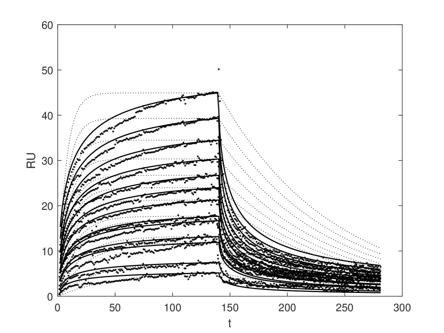
The data obtained from an SPR experiment is typically referred to as a sensorgram, which represents the system’s response proportional to the total complex concentration, measured over time for various analyte concentrations. The sensorgram for the system described in Section 3 is shown in Figure 7.
The sensorgram is divided into three distinct parts. During the association phase, the amount of complex formed () increases as a function of time until it reaches an equilibrium level. While the flow is maintained, the system remains in chemical equilibrium, and the complex concentration stays constant. When the analyte solution is replaced with a buffer solution, the analyte concentrations decreases to zero, initiating the dissociation process. After dissociation, the ligand and the analyte return to their original state as before binding. It is assumed that the system and experimental conditions are suitable for the kinetic model validity described in Section 2.2.
Typically, sensorgrams at varying concentrations of are fitted to obtain the association () and dissociation () constants. The experimental data are traditionally analyzed using a simple model fitting procedure. In the initial stage of the analysis, a nonlinear fit of the form is performed for values of . In this fit, the parameter is determined for each analyte concentration , with representing the maximum value of the response variable. In the subsequent step, under the assumption that , the curve is constructed, allowing for the determination of by the slope of the curve. To obtain the dissociation constant , a non-linear fit is performed for in which , thus is obtained for each . Subsequently, the average value of is taken. This is the standard method to fitting these data, as outlined in reference [41, 42, 22]. In this case, the values of and were found to be and , respectively. This result is designated as Case 1 in Table 1.
This paper proposes an alternative method for obtaining the constants. Considering that Equation (13) describes the three stages of the process, where ,, and .
| (19) |
The kinetic constants were determined by minimizing a nonlinear cost function, as defined in Equation (20).
| (20) |
In this case, only the sensorgram corresponding to a concentration of of was used in the adjustment process. To fit the model to the data, the maximum descent method was employed to minimize the sum of the relative least squares, calculated over the entire curve obtained at a concentration of . The values of and obtained from the previous strategy were used as a starting point. The resulting values were and , which are referred to as Case 2 in Table 1.
The values for the other concentrations, using the constants derived for , are also presented in Table 1. It is noteworthy that the results for cases 1 and 2 differ significantly, with Case 2 generally performing better. Table 1 shows that the constants and result in reduced for almost all values between and . The resulting in Case 2 was , compared to in Case 1.
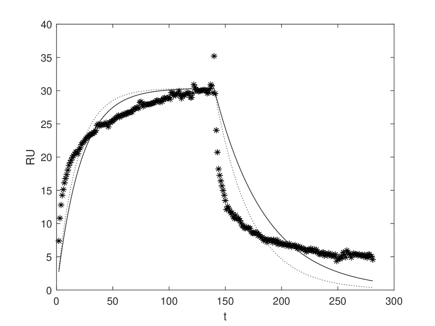
Figure 1 illustrates the fit of the integer-order model for both cases, respectively. Based on these observations, we conclude that, at least for this experimental data, Case 2 provides a better agreement between the kinetic model and the experimental data than Case 1.
The objective of this study is to determine whether the fractional model offers a more accurate representation of the experimental data.
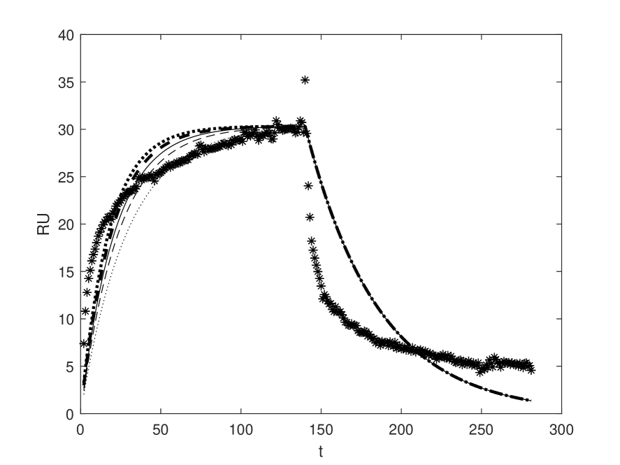
Before applying the fractional model, it is essential to examine the sensitivity of the kinetic constants. Figure 2 shows a study of the variation of . The solid line represents the result obtained by fitting the integer-order model using reference constants ( and ). The thick-dashed line illustrates the effect of a variation in (with held constant). Similarly, the dashed represents line a variation in , while the thick-dotted line shows the effect of a variation in , and the dotted line indicates a variation. The simulated changes in primarily affect the curve for , with no significant impact for . This result clearly indicates that adjusting the constant alone does not accurately capture the shape of the experimental curve.
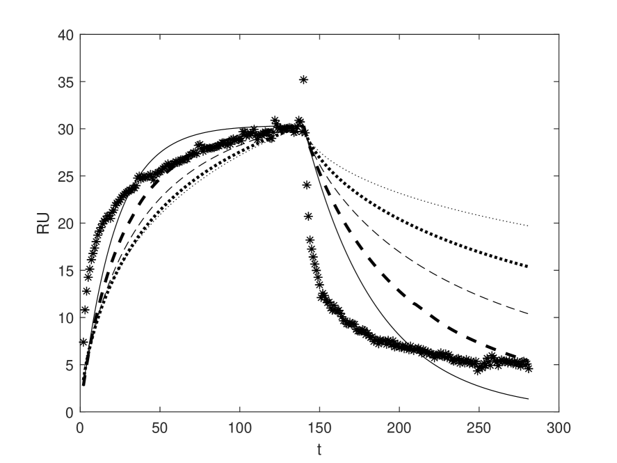
Similar study was conducted with constant, as shown in Figure 3. Again, the solid line represents the result obtained by fitting the integer-order model using the same reference constants. The thick-dashed line corresponds to a variation in , calculated as , while keeping constant. Similarly, the dashed line represents a variation in , the thick-dotted line indicates a , and the dotted line represents variation. The effects of varying are observed in both regions, and . However, the impact of these changes is more pronounced in the region. As previously noted in the study of , modifying the constant does not provide adequately represent the empirical curve when using the integer-order model.
Figures 2 and 3 illustrate that the integer-order model fails to accurately represent the experimental curve due to clear deviations from the exponential behavior. In the region, there is a rapid increase in , which then slows down until equilibrium is reached. In the region, decreases rapidly, faster than exponential, followed by a slower decline. This behavior suggests that a fractional model may be appropriate, as the Mittag-Leffler function is more flexible than the exponential function in accounting for these time-dependent differences. Therefore, improvements may only be realized by modifying the model.
An alternative model was employed:
| (21) |
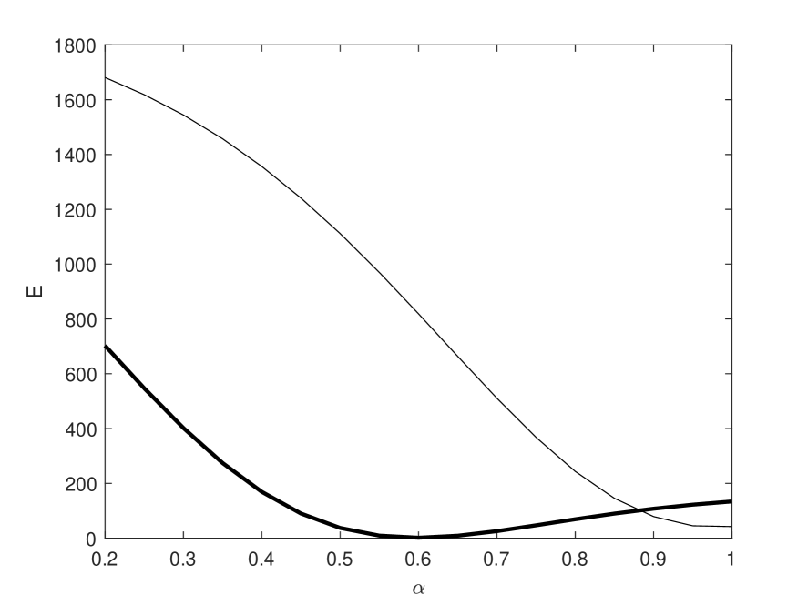
where is defined as before, , and . Figure 4 illustrates the effect of varying the fractional-order parameter , with and held constant. In Figure 4, the solid line represents the fit using . The thick-dashed line corresponds to , the dashed line to , the thick-dotted line to , and the dotted line to . These curves indicate that varying while keeping the constants fixed (i.e., a univariate parameter adjustment) does not improve the fit, as shown in Figure 4. Consequently, a multivariate adjustment was to implement. Figure 6 shows that, for specific values of and , there is an optimal . The thick line represents the cost function as a function of , using the and from Case 1. In this case, the value that minimizes is .
The next approach involved a multivariate adjustment by varying , , and , simultaneously, designated as Case 3. The same cost function was used. Here, the previously determined from the integer-order model was retained, while was increased by a factor of times, resulting in a new value of . Figure 5 presents the results. The adjustment yielded and , compared to for the integer-order model (), reducing the cost function value by a factor of .
The derivatives of integer-orders can be determined within infinitesimally small neighborhoods of the time point under consideration. This implies that such equations cannot described non-local effects. Fractional derivatives of non-integer-orders are employed in kinetic models to describe processes and systems that exhibit spatial and temporal non-locality, the latter often referred to as the “memory effect". “Memory" is a property of physical-chemistry processes in which the behavior of a process at a given specific time depends not only on the current state but on states over a finite or infinite past interval. This dependence on past states characterizes memory as an inherent property of such processes. When the influence extends beyond a single location, it is referred to as a non-local effect.
In the context of chemical reactions, interactions between distant molecules, such as dipole-dipole forces or van der Waals forces, can impact reaction processes over large distances. The memory effect can be defined as the influence of non-locality on the observed process. It has been shown that catalytic surfaces can exhibit memory effects related to the adsorption history of reactive molecules [43]. The state of the surface, including the presence of adsorbed species or morphological changes from previous exposures, can affect the efficiency of complex formation in subsequent cycles. Additionally, some reactions have demonstrate memory effects associated with the conformation of the ligand immobilized on the surface, which can influence the outcome of subsequent reactions [44]. In other words, the rate of a reaction at any given moment may depend on process history.
The fractional-order provide an alternative mean of achieving greater flexibility in the solution while maintaining the simplicity of the model. The fractional-order that best fit to the experimental curves was approximately . Figure (7) presents the sensorgrams for concentrations ranging from to . The experimental data are compared to the results obtained using the Case 3 strategy (thick continuous line). For all sensorgrams, optimal results were achieved using the Case 3 strategy, as shown in Table 1.
5 Conclusions
Over the past few decades, accelerated technological advancements have been made in biosensor instruments, such as Surface Plasmon Resonance (SPR) and Quartz Crystal Microbalance (QCM). These techniques enable real-time measurement of biomolecular interactions with high sensitivity.
The adsorption-desorption process observed through the SPR signal is complex and involves several concurrent phenomena. In this context, conventional kinetic models using first-order derivatives to describe the time evolution of the adsorption-desorption process are often insufficient for a detailed description. In this work, a model employing the Caputo fractional derivative was used to analyze the experimental data. The proposed model was applied to interaction data between Immobilized Baru Protein (IBP) and Congo Red (CR) dye at concentrations ranging from to , at pH 7.4 and 16 . A study of the variation of the kinetic constants showed that the integer-order model fails to adequately describe the experimental data.
In the filed of chemical reactions, there are examples where interactions between distant molecules, such as dipole-dipole forces or van der Waals forces, can significantly impact reaction processes, even over large distances. Moreover, certain reactions have been observed to exhibit memory effects associated with the conformation of ligands immobilized on surfaces, which can influence subsequent reactions. This means that the rate of a reaction at any given moment may depend on the process’s prior history. This study demonstrates that the fractional-order can effectively capture the complexity of such phenomena, offering a robust framework to account for non-local and memory-dependent effects.
The behavior observed in the experimental sensorgrams suggests that the Mittag-Leffler function provides greater flexibility than the exponential function in fitting the sensorgram’s shape over time. Using the fractional model, the cost function was reduced by a factor of 30, with and values comparable to those obtained from the integer-order model. These findings highlight the importance of further investigating the proposed fractional model to better understand the relationship between fractional-order kinetics and non-local phenomena.
Acknowledgments
This study was financed in part by the Coordenação de Aperfeiçoamento de Pessoal de Nível Superior (CAPES) - Finance Code 001, and Fundação de Amparo à Pesquisa do Estado de Minas Gerais (FAPEMIG).
| E() | |||
|---|---|---|---|
| Case 1 | Case 2 | Case 3 | |
| 7.5 | 31.7(1) | 42.3(1) | 19.0(0.5) |
| 15 | 54.8(1) | 39.4(1) | 22.8(0.55) |
| 22.5 | 18.6(1) | 47.1(1) | 5.75(0.45) |
| 30 | 62.3(1) | 39.2(1) | 4.25(0.55) |
| 37.5 | 67.0(1) | 38.0(1) | 2.24(0.55) |
| 45 | 134(1) | 40.6(1) | 3.37(0.6) |
| 52.5 | 126(1) | 40.3(1) | 5.33(0.55) |
| 60 | 157(1) | 39.2(1) | 1.74(0.6) |
| 67.5 | 225(1) | 44.8(1) | 2.26(0.6) |
| 75 | 183(1) | 42.3(1) | 1.52(0.6) |
| 82.5 | 214(1) | 43.9(1) | 3.04(0.6) |
| 90 | 255(1) | 45.8(1) | 2.56(0.6) |
| 97.5 | 273(1) | 45.9(1) | 3.34(0.6) |


References
- [1] HOMOLA, J. Surface Plasmon Resonance Sensors for Detection of Chemical and Biological Species. Chemical Reviews, v. 108, n. 2, p. 462-493, 1 fev. 2008.
- [2] KARLSSON, R. et al. Kinetic and Concentration Analysis Using BIA Technology. Methods, v. 6, n. 2, p. 99-110, jun. 1994.
- [3] KILBAS, A. A.; SRIVASTAVA, H. M.; TRUJILLO, J. J. Theory and applications of fractional differential equations. 1st ed ed. Amsterdam; Boston: Elsevier, 2006.
- [4] LEMES, N. H. T.; DOS SANTOS, J. P. C.; BRAGA, J. P. A generalized Mittag-Leffler function to describe nonexponential chemical effects. Applied Mathematical Modelling, v. 40, n. 17-18, p. 7971-7976, set. 2016.
- [5] PODLUBNY, I. Fractional differential equations: an introduction to fractional derivatives, fractional differential equations, to methods of their solution and some of their applications. San Diego: Academic Press, 1999.
- [6] MONTEIRO, N. Z.; DOS SANTOS, R. W.; MAZORCHE, S. R. Constructive fractional models through Mittag-Leffler functions. Computational and Applied Mathematics, v. 43, n. 4, p. 177, jun. 2024.
- [7] ZERAICK MONTEIRO, N.; WEBER DOS SANTOS, R.; RODRIGUES MAZORCHE, S. Bridging the gap between models based on ordinary, delayed, and fractional differentials equations through integral kernels. Proceedings of the National Academy of Sciences, v. 121, n. 19, p. e2322424121, 7 maio 2024.
- [8] NISAR, K. S. et al. A review of fractional order epidemic models for life sciences problems: Past, present and future. Alexandria Engineering Journal, v. 95, p. 283-305, maio 2024.
- [9] BEYLE, A.; IBEH, C. C. Predicting the viscoelastic behavior of polymer nanocomposites. Em: Creep and Fatigue in Polymer Matrix Composites. [s.l.] Elsevier, 2011. p. 184-233.
- [10] DOKOUMETZIDIS, A.; MACHERAS, P. Fractional kinetics in drug absorption and disposition processes. Journal of Pharmacokinetics and Pharmacodynamics, v. 36, n. 2, p. 165-178, abr. 2009.
- [11] MAINARDI, F. Why the Mittag-Leffler Function Can Be Considered the Queen Function of the Fractional Calculus? Entropy, v. 22, n. 12, p. 1359, 30 nov. 2020.
- [12] HOWELL, D. (ED.). Surface plasmon resonance (SPR): advances in research and applications. New York: Nova Science Publishers, 2017.
- [13] SINGH, P. (ED.). Surface plasmon resonance. New York: Novinka, 2014.
- [14] SCHASFOORT, R. B. M. (ED.). Handbook of surface plasmon resonance. 2nd edition ed. London: Royal Society of Chemistry, 2017.
- [15] SANVICENS, N. et al. Biosensors for pharmaceuticals based on novel technology. TrAC Trends in Analytical Chemistry, v. 30, n. 3, p. 541?553, mar. 2011.
- [16] DAMBORSKÝ, P.; VITEL, J.; KATRLÍK, J. Optical biosensors. Essays in Biochemistry, v. 60, n. 1, p. 91-100, 30 jun. 2016.
- [17] GAUDREAULT, J. et al. On the Use of Surface Plasmon Resonance-Based Biosensors for Advanced Bioprocess Monitoring. Processes, v. 9, n. 11, p. 1996, 9 nov. 2021.
- [18] KRETSCHMANN, E.; RAETHER, H. Notizen: Radiative Decay of Non Radiative Surface Plasmons Excited by Light. Zeitschrift für Naturforschung A, v. 23, n. 12, p. 2135?2136, 1 dez. 1968.
- [19] RITCHIE, R. H. Plasma Losses by Fast Electrons in Thin Films. Physical Review, v. 106, n. 5, p. 874-881, 1 jun. 1957.
- [20] STENBERG, E. et al. Quantitative determination of surface concentration of protein with surface plasmon resonance using radiolabeled proteins. Journal of Colloid and Interface Science, v. 143, n. 2, p. 513?526, maio 1991.
- [21] DAY, Y. S. N. et al. Direct comparison of binding equilibrium, thermodynamic, and rate constants determined by surface and solution based biophysical methods. Protein Science, v. 11, n. 5, p. 1017-1025, maio 2002.
- [22] AGUIAR, C. D. D. et al. Thermodynamic and kinetic insights into the interactions between functionalized CdTe quantum dots and human serum albumin: A surface plasmon resonance approach. International Journal of Biological Macromolecules, v. 184, p. 990-999, ago. 2021.
- [23] FILIPPOVA, N. L. Kinetic-Diffusion-Controlled Adsorption and Desorption Kinetics on Planar Surfaces. Journal of Colloid and Interface Science, v. 206, n. 2, p. 592-602, out. 1998.
- [24] OLIVEIRA, E. C. DE. Solved exercises in fractional calculus. Cham: Springer, 2019.
- [25] ROSS, B. (ED.). Fractional Calculus and Its Applications: Proceedings of the International Conference Held at the University of New Haven, June 1974. Berlin, Heidelberg: Springer Berlin Heidelberg, 1975. v. 457.
- [26] DIETHELM, K. The Analysis of Fractional Differential Equations: An Application-Oriented Exposition Using Differential Operators of Caputo Type. Berlin, Heidelberg: Springer Berlin Heidelberg, 2010. v. 2004.
- [27] GARRAPPA, R.; GIUSTI, A.; MAINARDI, F. Variable-order fractional calculus: a change of perspective. 2021.
- [28] CAPUTO, M. Linear Models of Dissipation whose Q is almost Frequency Independent–II. Geophysical Journal International, v. 13, n. 5, p. 529?539, 1 nov. 1967.
- [29] GORENFLO, R. et al. Mittag-Leffler Functions, Related Topics and Applications: Theory and Applications. Berlin, Heidelberg: Springer Berlin Heidelberg, 2014.
- [30] DE OLIVEIRA, E. C. Sobre a clássica função de Mittag-Leffler. Revista Matemática Universitária, v. 1, n. 01, 2020.
- [31] BEGHIN, L.; CAPUTO, M. Commutative and associative properties of the Caputo fractional derivative and its generalizing convolution operator. Communications in Nonlinear Science and Numerical Simulation, v. 89, p. 105338, out. 2020.
- [32] SALES TEODORO, G.; TENREIRO MACHADO, J. A.; CAPELAS DE OLIVEIRA, E. A review of definitions of fractional derivatives and other operators. Journal of Computational Physics, v. 388, p. 195-208, jul. 2019.
- [33] ORTIGUEIRA, M. D.; TENREIRO MACHADO, J. A. What is a fractional derivative? Journal of Computational Physics, v. 293, p. 4-13, jul. 2015.
- [34] ANGSTMANN, C. N. et al. A General Framework for Fractional Order Compartment Models. SIAM Review, v. 63, n. 2, p. 375-392, jan. 2021.
- [35] ARFKEN, G. B.; WEBER, H.-J.; HARRIS, F. E. Mathematical methods for physicists: a comprehensive guide. 7th ed ed. Amsterdam; Boston: Elsevier, 2013.
- [36] HAUBOLD, H. J.; MATHAI, A. M.; SAXENA, R. K. Mittag-Leffler Functions and Their Applications. Journal of Applied Mathematics, v. 2011, n. 1, p. 298628, jan. 2011.
- [37] JUMARIE, G. Laplace’s transform of fractional order via the Mittag-Leffler function and modified Riemann-Liouville derivative. Applied Mathematics Letters, v. 22, n. 11, p. 1659?1664, nov. 2009.
- [38] SUN, H. et al. A Review on Variable-Order Fractional Differential Equations: Mathematical Foundations, Physical Models, Numerical Methods and Applications. Fractional Calculus and Applied Analysis, v. 22, n. 1, p. 27?59, fev. 2019.
- [39] PATNAIK, S.; HOLLKAMP, J. P.; SEMPERLOTTI, F. Applications of variable-order fractional operators: a review. Proceedings of the Royal Society A: Mathematical, Physical and Engineering Sciences, v. 476, n. 2234, p. 20190498, fev. 2020.
- [40] PATNAIK, S.; HOLLKAMP, J. P.; SEMPERLOTTI, F. Applications of variable-order fractional operators: a review. Proceedings of the Royal Society A: Mathematical, Physical and Engineering Sciences, v. 476, n. 2234, p. 20190498, fev. 2020.
- [41] ARAUJO MARQUES, I. et al. Exploring the Recognition Mechanism of Surfactant Cyclodextrin Complex Formation: Insights from SPR Studies on Temperature and Ionic Liquid Influence. The Journal of Physical Chemistry B, p. acs.jpcb.4c04516, 20 set. 2024.
- [42] DE CASTRO, A. S. B. et al. Kinetic and thermodynamic of lactoferrin Ethoxylated-nonionic surfactants supramolecular complex formation. International Journal of Biological Macromolecules, v. 187, p. 325-331, set. 2021.
- [43] FENG, X. et al. A review on heavy metal ions adsorption from water by layered double hydroxide and its composites. Separation and Purification Technology, v. 284, p. 120099, fev. 2022.
- [44] SMITH, B. J. et al. Metal complex assembly controlled by surface ligand distribution on mesoporous silica: Quantification using refractive index matching and impact on catalysis. Journal of Catalysis, v. 335, p. 197-203, mar. 2016.