Controlled Model Debiasing through Minimal and Interpretable Updates
Abstract
Traditional approaches to learning fair machine learning models often require rebuilding models from scratch, generally without accounting for potentially existing previous models. In a context where models need to be retrained frequently, this can lead to inconsistent model updates, as well as redundant and costly validation testing. To address this limitation, we introduce the notion of controlled model debiasing, a novel supervised learning task relying on two desiderata: that the differences between new fair model and the existing one should be (i) interpretable and (ii) minimal. After providing theoretical guarantees to this new problem, we introduce a novel algorithm for algorithmic fairness, COMMOD, that is both model-agnostic and does not require the sensitive attribute at test time. In addition, our algorithm is explicitly designed to enforce (i) minimal and (ii) interpretable changes between biased and debiased predictions—a property that, while highly desirable in high-stakes applications, is rarely prioritized as an explicit objective in fairness literature. Our approach combines a concept-based architecture and adversarial learning and we demonstrate through empirical results that it achieves comparable performance to state-of-the-art debiasing methods while performing minimal and interpretable prediction changes.
1 Introduction
The increasing adoption of machine learning models in high-stakes domains—such as criminal justice (Kleinberg et al., 2016) and credit lending (Bruckner, 2018)—has raised significant concerns about the potential biases that these models may reproduce and amplify, particularly against historically marginalized groups. Recent public discourse, along with regulatory developments such as the European AI Act (2024/1689), has further underscored the need for adapting AI systems to ensure fairness and trustworthiness (Bringas Colmenarejo et al., 2022). Consequently, many of the machine learning models deployed by organizations are, or may soon be, subject to these emerging regulatory requirements. Yet, such organizations frequently invest significant resources (e.g. time and money) in validating their models with the assistance of domain experts before deploying them at scale (see, e.g., (Mata et al., 2021) for dam safety monitoring and (Tsopra et al., 2021) for precision medicine), to ensure their performance and trustworthiness. As new regulatory constraints emerges for these models, the ability to make these models comply with new constraints while minimizing the need for revalidation has thus become critically important.
The field of algorithmic fairness has experienced rapid growth in recent years, with numerous bias mitigation strategies proposed (Romei & Ruggieri, 2014; Mehrabi et al., 2021). These approaches can be broadly categorized into three types: pre-processing (e.g.,(Belrose et al., 2024)), in-processing (e.g.,(Zhang et al., 2018)), and post-processing (e.g., (Kamiran et al., 2010)), based on the stage of the machine learning pipeline at which fairness is enforced. While the two former categories do not account at all for any pre-existing biased model being available for the task, post-processing approaches aim to impose fairness by directly modifying the predictions of a biased classifier. This thus naturally imposes some kind of consistency between the new, fair model and the old, biased one. However, these methods are generally deemed to achieve lower performance, and the changes performed are generally not traceable.
Motivated by these considerations, in this paper we consider a new paradigm, proposing to frame algorithmic fairness as a model update task. The goal is thus to enforce fairness through small and understandable, updates to a pretrained, presumably biased, model, in order to facilitate model monitoring. For this purpose, we introduce the notion of Controlled Model Debiasing, based on two intuitive desiderata: (i) changes between the new model and the existing one should be minimal, and (ii) these changes should be understandable. This formulation combines assumptions from both post-processing (e.g., (Kamiran et al., 2010)) and in-processing (e.g., (Zhang et al., 2018)) approaches, proposing to learn a new fair model by leveraging a previously trained biased one. After providing theoretical guarantees on the solution and feasibility of this new proposed problem, we introduce COMMOD (COncept-based Minimal MOdel Debiasing), our method to address it. Leveraging the fields of concept-based interpretability (Alvarez Melis & Jaakkola, 2018; Koh et al., 2020b) and fair adversarial learning (Zhang et al., 2018; Grari et al., 2021), COMMOD is a model-agnostic, interpretable debiasing method that aims to improve fairness in an interpretable way, while minimizing prediction changes relative to the original model. Through experiments, we demonstrate that our method achieves comparable fairness and accuracy performance to existing algorithmic fairness approaches, while requiring fewer prediction changes. Additionally, we show that COMMOD enables more meaningful and easier-to-understand prediction changes, enhancing its utility in practice. To summarize, our contributions are as follows:
-
•
We introduce a new notion of Controlled Model Debiasing, which aims to account for a previously trained model by performing minimal and interpretable updates to mitigate bias (Section 3). To the best of our knowledge, we are the first to address interpretability directly in the updating process. Previously, only post-hoc interpretation of the debiasing process (e.g., (Ţifrea et al., 2023)) has been explored.
-
•
We provide two theoretical guarantees for the proposed problem: the formulation of the Bayes-Optimal Classifier in a fairness-aware setting and the feasibility of the problem in the general setting (Section 4).
-
•
We introduce a new method, COMMOD, to address the new optimization problem in a model-agnostic, fairness-unaware setting (Section 5). We validate its performance through experiments on classical fairness datasets, showcasing its debiasing efficacy and ability to perform fewer and more interpretable changes (Section 6).
2 Background and notation
Let be an input space consisting of features and an output space. In a traditional algorithmic fairness framework in supervised learning, we want an algorithm that outputs such that is unbiased from a sensitive variable , only available at training time. For the sake of simplicity, we focus in this paper on a binary classification problem where and for which also the sensitive attribute takes values on a binary sensitive space .
2.1 Group fairness
Over the years, several notions of fairness have been proposed in the literature to define whether or not a variable is unbiased from a sensitive variable ((Dwork et al., 2012; Hardt et al., 2016; Jiang et al., 2020)). In this paper, we focus on two of the most used ones: Demographic Parity (Calders et al., 2009) and Equalizing Odds (Hardt et al., 2016).
2.1.1 Demographic Parity
A classifier satisfies Demographic Parity (DP) if the prediction is independent from sensitive attribute . In the case of a binary classification, this is equivalent to Hence, Demographic Parity can be measured using the P-rule:
2.1.2 Equalizing Odds
A classifier satisfies Equalizing Odds (EO) if the prediction is conditionally independent of the sensitive attribute given the actual outcome . In the case of a binary classification problem, this is equivalent to for all . Hence, Equalizing Odds can be measured using the Disparate Mistreatment (DM) (Zafar et al., 2017):
where and . In the rest of the paper, we use .
2.2 Mitigation strategies
Bias mitigation algorithms are generally grouped into three different categories, based on when the debiasing process is carried on in the machine learning pipeline (Romei & Ruggieri, 2014). In particular, pre-processing methods (e.g. (Zemel et al., 2013)) modify the training data such that they are unbiased with respect to . In-processing methods (e.g. (Zhang et al., 2018)) aim to train a new, fair, classifier by integrating some fairness constraints in the optimization objective. Finally, post-processing methods approaches aim to achieve fairness by adjusting the predictions of an already existing model . Hence, post-processing methods learn a function that maps into fairer predictions . As such, a notion of predictive similarity between these two sets of predictions often being optimized, either directly (Jiang et al., 2020; Nguyen et al., 2021; Alghamdi et al., 2022) or indirectly through heuristics (Kamiran et al., 2018). However, rather than an assumed end-goal, this objective generally remains a proxy for the true goal of optimizing accuracy, as the true labels are generally assumed to be unavailable at inference time in the post-processing setting. Furthermore, these approaches generally suffer from several limitations, such as not being model-agnostic (Calders & Verwer, 2010; Kamiran et al., 2010; Du et al., 2021), or requiring access to the sensitive attribute at test time (Hardt et al., 2016; Pleiss et al., 2017), which greatly hurt their practical use. On this topic, we provide a review of existing post-processing approaches and their limitations in Table 1 in Appendix.
3 Controlled model debiasing
Let us now consider a context where a model needs to be updated with a model . In addition to maintaining its accuracy, the objective is to make it fairer with respect to a specific fairness definition discussed in Section 2.1. As discussed in Sec. 1, blindly training can be harmful for several reasons. First, Krco et al. (2023) have shown that some bias mitigation approaches performed needlessly large numbers of prediction changes for similar levels of accuracy and fairness. Yet, a large number of inconsistent decisions may negatively impact users’ trust, as shown by Burgeno & Joslyn (2020) in the context of weather forecast. On top of this, beyond statistical testing, models in production may undergo extensive testing by domain experts Tsopra et al. (2021). In this context, being able to understand the changes from one model to the other would be crucial to not being forced to undergo all the testing again, in addition to increasing expert trust.
Driven by the above-mentioned considerations, we introduce the notion of Controlled Model Update, which is based on the following notions of Interpretable and Minimal updates.
3.1 Interpretable updates
To facilitate the adoption of a new model , we propose to generate explanations that describe how the debiasing process modified the old model . Contrary to traditional XAI methods (see, e.g. (Guidotti et al., 2018) for a survey), rather than explaining the decisions of the model , our aim here is to generate insights about the differences between and . An intuitive solution to this problem would be to first train a fair model and then generating explanations for these differences in a post-hoc manner, akin to (Renard et al., 2024). However, post hoc interpretability methods, in general, are often criticized for their lack of connection with ground-truth data (Rudin, 2019; Laugel et al., 2019). Therefore, in order to ensure better trust in the new model, we pursue the direction of self-explainable models (Alvarez Melis & Jaakkola, 2018), generating global explanations for the differences between and while learning the predictive task.
3.2 Minimal updates
The constraint of ensuring that the new model remains as similar as possible to the initial one can be directly added to the training objective (e.g. the one in (Zhang et al., 2018)). In particular, to the usual optimization problem of fairness, we added a constraints that control the probability for a prediction to change label after the debiasing process. We emphasize once again that making minimal changes to a biased model is beneficial in cases where the model has already been validated based on user needs. Significant updates to make the model fairer might risk no longer satisfying those needs, requiring once again a costly validation.
We then frame our problem in a traditional algorithmic-fairness way, in which the self-explainable model is required to be accurate and fair. On top of these constraints, is required to be similar to in terms of predicted classes. The combination of these desiderata allows us to understand what changes are required from a biased model to become fairer focusing on minimal adjustments.
Let be the fairness criteria (e.g. Demographic Parity or Equalizing Odds). Further, let us define the predictions of the biased model and edited model as and respectively. We can then formalize our optimization problem through the following Controlled Model Update objective:
| (1) | ||||
| s.t. | ||||
where and . Observe that setting , i.e. forbidding any prediction change to happen, imposes . On the contrary, the more increases and the more is free to differ from and, ideally, to reach higher fairness scores. When , Eq. 1 becomes a classical algorithmic fairness learning problem. Notice also that the interpretability is all carried by the self-explainable model itself, and hence it will be not explicitly appear in the optimization problem of Equation 1. We will discuss our self-explainable model in Section 5.2.
4 Theoretical guarantees on the minimal update problem
In this section, we present two theoretical contributions to the problem formalized in Eq. 1. First (Sec. 4.1), we show that it is possible to define the Bayes Optimal Classifier of the problem in the fairness-aware setting. Then, in Section 4.2, we assess the feasibility of the problem in general, giving guarantees on the trade-off between fairness and number of prediction changes. All proofs can be found in Appendix C.
4.1 Result 1: Bayes-optimal classifier in a fairness-aware setting
Let be a joint distribution on , where is the instance, the target feature, the sensitive variable, and the output of the black-box classifier. Let be the distribution over , a suitable distribution (DP or EO) over and a distribution over . We want to show that despite the new constraint on the number of changes, our optimization problem in Eq. 1 still has an analytical solution (i.e. the Bayes-optimal classifier (BOC)) in a fairness aware setting knowing the true distributions above mentioned.
To do so, we leverage the work of (Menon & Williamson, 2018), who defined the BOC in the traditional fairness setting, relying on a reformulation of the optimization problem using the notion of cost-sensitive risk111From (Menon & Williamson, 2018): The risk of a randomized classifier computed on is called cost sensitive risk for a cost parameter and if it can be written as
where and . For what concerns the fairness constraint, they show (Lemma 3) that is equivalent to , where
is the balanced cost-sensitive risk and .
Following the same idea, we first establish the equivalence between the constraint on the number of changes and a cost-sensitive risk:
Lemma 4.1.
Pick any random classifier . Then, for any ,
with 222Notice that we changed the distribution w.r.t. FPR and FNR are computed. Hence, and .
Finally, in a similar fashion of the main result in (Menon & Williamson, 2018) about the Bayes-Optimal Classifier, we can define for any cost the Lagrangian of the optimization problem in Eq. 1 as:
| (2) | ||||
Proposition 4.2 (Fairness-aware Bayes-optimal classifier).
The Bayes optimal classifier of in a fairness aware setting and knowing the distributions is given by
where and is the modified Heaviside (or step) function for a parameter .
Despite its theoretical importance, the BOC presented in Proposition 3.2 remains impractical for computation, as the joint and marginal distributions of the random variables are typically inaccessible in real-world applications. Furthermore, the above result only holds within a fairness-aware setting, a context that is uncommon in practical scenarios. For this reason, we introduce in Sec. 5 a novel algorithm that optimizes a relaxed form of the optimization problem in Eq. 1, which does not require knowledge of the sensitive attribute at test time.
4.2 Result 2: fairness level under a maximum change constraint
We now aim to theoretically understand what happens experimentally to the trade-off between fairness score (DP in this case) and the similarity between and defined in Eq. 1. For this purpose, we study the impact that changes to the predictions of can have on the P-Rule.
We start by defining the following notations, used to divide a set of instances based on the values of their outcomes and of their sensitive attribute :
Using this notation, the P-Rule is experimentally measured as , where is a fixed and not editable constant that depends on the population’s distribution with respect to the binary sensitive attribute. Further, without loss of generality, we now suppose that , i.e. . Hence, in order to increase the P-Rule to a higher value with changes on the predictions, i.e. by modifying the set into the set , two types of actions on and could be performed:
-
(a)
Increasing (i.e. changing the prediction of individuals belonging to the minority group from to ).
-
(b)
Decreasing (i.e. changing the prediction of individuals belonging to the majority group from to ).
Note that both these two actions could lead to a switch in the minimum of the definition of P-Rule in the sense that from one could arrive at . This is due to the fact that when one instance of the minimum decreases, the other one increases. Let us consider an algorithm that, given , only plays a strategy that is either (a), (b) or a combination of the two. For such an algorithm, we can introduce the following definition.
Definition 4.3.
(Switching point) The switching point of an algorithm of the type above is the number of changes required to get a .
Informally, this is the number of changes required to get , where the approximation is needed because the quantities are integer values and in general. With this in mind, we can prove the following proposition:
Proposition 4.4.
Let an algorithm of the type above. Then, given changes with , the maximum P-Rule we can get is given by an algorithm that always plays action (a) or always action (b).
The only thing one should keep in mind is that by doing changes one needs to have either enough instances falling into (if we increase the numerator) or into (if we decrease the denominator).
We believe this result represents a significant milestone in the theoretical characterization of the effects of debiasing a model using DP as a fairness measure. Although this result provides valuable insights into the dynamics of the debiasing process, Proposition 4.4 does not account for the potential impact of these optimal changes on model accuracy. This highlights the possibility that, in the context of algorithmic fairness—where the goal is to balance fairness and accuracy—debiasing algorithms may prioritize alternative changes that minimize adverse effects on accuracy. On top of this, this theoretical result would be algorithmically applicable only in a fairness aware setting due to the fact that the knowledge of proportion is required. To this goal, we evaluate the performances of an algorithm of the type above in the Appendix C.2.1.
5 COMMOD: an algorithm for controlled model debiasing
As previously mentioned, while the BOC of Proposition 4.2 is theoretically relevant in the Fairness-Aware setting, it lacks practical utility. In order to solve Problem 1, we thus propose a new algorithm, called COMMOD, circumventing these limitations and integrating the interpretability objective described in Section 3. COMMOD aims to edit the probabilities scores of the biased model into scores , whose associated predictions are more fair. The update is done through a multiplicative factor as follows:
| (3) |
where is the sigmoid function to ensure and is the logit value of the biased model . Besides being intuitive, this formulation enables a more direct modelling of the differences between and , as . We then propose to model the ratio as a Neural Network with parameters and taking as input . In the subsections below, we describe how both desiderata of similarity and interpretability are integrated in COMMOD.
5.1 Penalization term for minimal updates
We propose to minimize model changes by adding a penalization term . Numerous similarity measures between and can be considered, depending on the considered scenario: for instance, existing works in post-processing fairness generally focus on distances between distributions such as the Wasserstein distance (Jiang et al., 2020) or the KL-divergence (Ţifrea et al., 2023). Here, we propose to use either a mean squared norm function defined by a positive-definite inner product . This term ensure that the score is not modified unnecessarily, and thus that the calibration of remains consistent (cf. Figure 9 in App. E.4 for a related discussion). For the sake of simplicity, in the experiments of our paper we set , recovering the classical Euclidean distance.
5.2 Concept-based Architecture for Interpretable Changes
In our approach, we prioritize interpretability by utilizing a self-explainable model. For classification problems, interpretable models par excellence are decision trees. On the other hand, for regression we do not have the same theoretical understanding but a model that is usually considered interpretable is Sparse Linear Regression. On top of that, inspired by the growing body of works on concepts (Koh et al., 2020a; Yuksekgonul et al., 2023; Fel et al., 2023; Zarlenga et al., 2023), we propose to learn concepts in an unsupervised manner where every concept is a sparse linear combination of the input features. Consistently with previous works, we also posit that these concepts should be both diverse (Alvarez Melis & Jaakkola, 2018; Fel et al., 2023; Zarlenga et al., 2023) to be meaningful and the least redundant possible. Hence, the model is interpretable due to the structure of that is a neural network without activation functions. The final architecture consists of an initial (linear) bottleneck that maps the input features into concepts, followed by an output layer that linearly combines these concepts to produce the multiplicative ratio needed for the update. By using linear combinations for both the features-to-concepts mapping and the concepts-to-output mapping, we can directly examine the learned weights to understand the direction (positive or negative) in which each concept—and, by extension, each feature—contributes to the value of the ratio. This level of interpretability was not achievable in previous models like TabCBM (Zarlenga et al., 2023). To ensure that the learned concepts are meaningful, we introduce penalization terms for diversity and sparsity, similar to those in (Zarlenga et al., 2023). Given our linear architecture, these terms are defined as follows: for sparsity, we use a Lasso penalization term, and for diversity, we define the penalization as , where denotes the cosine distance and are the network’s weights from input features to concepts and respectively. The combined penalization term is then given by .
5.3 Final model
To ensure fairness, we propose to leverage the technique proposed by (Zhang et al., 2018), which relies on a dynamic reconstruction of the sensitive attribute from the predictions using an adversarial model to estimate and mitigate bias. The higher the loss of this adversary is, the more fair the predictions are. Furthermore, this allows us to mitigate bias in a fairness-blind setting (i.e. without access to the sensitive attribute at test time), thus overcoming the limitation of most post-processing fairness methods (cf Table 1). Thus, the relaxed version of Equation 1 for DP can be written as:
| (4) | |||
with . In practice, we relax Problem 4, integrating the interpretability constraints on the concepts:
| (5) | ||||
with , and three hyperparameters. Similarly to (Zhang et al., 2018) this loss function can easily be adapted to address EO by modifying the adversary to take as both the true labels and the predictions .
6 Experiments
After describing our experimental setting, we propose in this section to empirically evaluate the two dimensions of the controlled model update: the ability to achieve accuracy and fairness with minimal (Section 6.2), and interpretable (Section 6.3) prediction changes.
6.1 Experimental protocol
6.1.1 Datasets
6.1.2 Competitors and baselines
To assess the efficacy of COMMOD, we first use an in-processing debiasing method, AdvDebias (Zhang et al., 2018), described in Section 2.1. We use the implementation provided in the AIF360 library (Bellamy et al., 2018). Additionally, as discussed in Section 6.2, post-processing debiasing methods also use a pretrained classifier as input. Yet, most methods are not directly comparable as they are not model-agnostic or require the sensitive attribute a test time. Two exceptions are LPP (Xian & Zhao, 2024) and FRAPPE (Ţifrea et al., 2023), which we use as competitors. Furthermore, although not directly comparable, we include the fairness-aware algorithms proposed by (Xian & Zhao, 2024) (that we name "Oracle (LPP)") and (Kamiran et al., 2012) ("Oracle (ROC)) as baselines. As they directly use the sensitive attribute to make predictions, these two algorithms are expected to outperform all the others.
6.1.3 Set-up
After splitting each dataset in () and (), we train our pretrained classifier to optimize solely accuracy. In these experiments, we use a Logistic Regression classifier from the scikit-learn library, but any other classifier could be used since COMMOD and the proposed competitors are model-agnostic. We then train COMMOD, the competitors and the baselines on , varying hyperparameter values for each method to achieve a range of fairness and accuracy scores over . For COMMOD, we set a fixed value for the number of concepts : for Law School and for Compas. Further details on implementation are available in Section D of the Appendix.
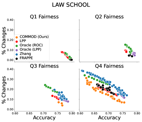
6.2 Experiment 1: achieving fairness through minimal changes
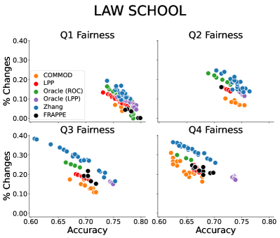
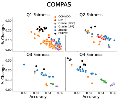
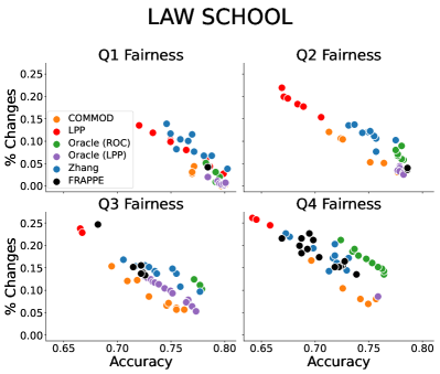
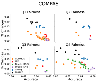
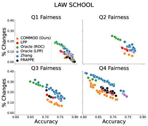
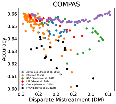
In this first experiment, we aim to assess the ability of COMMOD to achieve competitive results in terms of fairness and accuracy while performing a lower number of changes. For this purpose, we measure the proportion of prediction changes between the black-box model and the fairer model on the test set . As this value is directly linked to the fairness and accuracy levels of the models, we intend to evaluate for models with comparable levels of fairness and accuracy. To do so, we discretize the fairness scores into four segments, defined as quartiles of the scores of : Q1 corresponds to the most biased models, and Q4 to the most fair ones. The full details of these segments are available in Appendix D.2, along with a robustness analysis (cf. Appendix E.1) in which, to ensure that our results do not depend on the specific segment definition chosen, we reproduce the same experiment with other segment definitions. For each segment, we then display the Pareto graph between (y-axis, lower is better) and Accuracy (x-axis, higher is better) in Figure 1: in this representation, the most efficient method will be the closest one to the bottom left corner.
We observe that for similar levels of accuracy and fairness, COMMOD consistently achieves lower values of number of changes than its competitors. For less fair models (segment Q1), the difference is more subtle: as models put less emphasis on fairness than on accuracy, they tend to adopt a similar behavior, i.e. the one of the biased model . In other segments however, the value of COMMOD is more notable.
6.3 Experiment 2: interpretability of the model updates
In this second experiment, we aim to evaluate the quality of the explanations generated with COMMOD.
6.3.1 Illustrative results
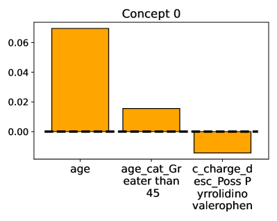
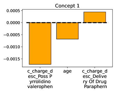
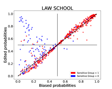
Starting with an example of explanation on the Compas Dataset. After training COMMOD with concepts, we obtain a final test P-Rule score of (up from with ) and accuracy of (down from ) with . The first two plots of Figure 2 highlight the diversity between these concepts, as they target different features. For instance, the concept , contributing positively () to class changes, is primarily activated by older individuals; on the other hand, , contributing negatively (), targets a specific crime category. In the third graph, we calculate the probability values in the sets corresponding to the instances activated by the corresponding features. Although preliminary, these observations show the potential of COMMOD to explain the debiasing process.
6.3.2 Quantitative results
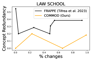
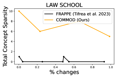
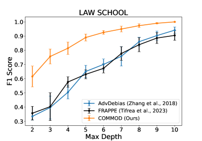
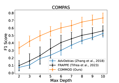
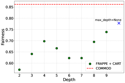
We now aim to generalize the previous observation by verifying that the concepts learned are diverse and sparse over the features of . To assess sparsity, we evaluate the total concept sparsity computed by summing across concepts the sparsity of each matrix after applying a threshold of : . For diversity, we measure the Jaccard Index between the signed non-null coefficients: diverse concepts may still use the same feature of if said feature contribution is in the opposite direction. As a baseline, we compare COMMOD (with ) with FRAPPE (Ţifrea et al., 2023), when the latter is trained using a linear network with the same architecture as the one used for our ratio for their additive term. Figure 3, highlights that for all levels of number of changes, the concepts learned using COMMOD are indeed more sparse and diverse as expected. Finally, we aim to show that the instances targeted by COMMOD are generally located in regions that are easier to interpret. In classification, there exists a theoretical understanding on how a class of models is interpretable based on how it can be translated into a decision tree (Bressan et al., 2024). Driven by this work, we propose a new evaluation protocol relying on measuring the accuracy of a decision tree of constrained depth trained to predict whether an instance has its prediction changed or not (i.e. on labels ). The idea behind this evaluation protocol is that a decision tree with a constrained depth will more accurately model prediction changes if these changes can be described with a lower number of features, and if these instances are more concentrated in the feature space. We report in Figure 4 the F1 scores of the decision trees trained to predict the class changes of COMMOD, FRAPPE and AdvDebias. We observe that for all values of maximum tree depth considered, thanks to the regularization with , the predictions changed by COMMOD are indeed much easier to interpret with a decision tree.
7 Conclusion
In this work, we introduced COMMOD, a novel model update technique that manages to enforce fairness and accuracy while making less, and more interpretable, changes to the original biased classifier. Additionally, we also provided theoretical results for this new optimization problem. Future works include researching the Controlled Model Debiasing task in non-linear settings, and further exploring the tradeoffs between the different hyperparameters to propose automated selection strategies.
References
- Alghamdi et al. (2022) Wael Alghamdi, Hsiang Hsu, Haewon Jeong, Hao Wang, P Winston Michalak, Shahab Asoodeh, and Flavio P Calmon. Beyond adult and compas: Fairness in multi-class prediction. arXiv preprint arXiv:2206.07801, 2022.
- Alvarez Melis & Jaakkola (2018) David Alvarez Melis and Tommi Jaakkola. Towards robust interpretability with self-explaining neural networks. Advances in neural information processing systems, 31, 2018.
- Angwin et al. (2016) Julia Angwin, Jeff Larson, Surya Mattu, and Lauren Kirchner. Machine bias. ProPublica, May 23, 2016, 2016.
- Bellamy et al. (2018) Rachel K. E. Bellamy, Kuntal Dey, Michael Hind, Samuel C. Hoffman, Stephanie Houde, Kalapriya Kannan, Pranay Lohia, Jacquelyn Martino, Sameep Mehta, Aleksandra Mojsilovic, Seema Nagar, Karthikeyan Natesan Ramamurthy, John Richards, Diptikalyan Saha, Prasanna Sattigeri, Moninder Singh, Kush R. Varshney, and Yunfeng Zhang. AI Fairness 360: An extensible toolkit for detecting, understanding, and mitigating unwanted algorithmic bias, October 2018.
- Belrose et al. (2024) Nora Belrose, David Schneider-Joseph, Shauli Ravfogel, Ryan Cotterell, Edward Raff, and Stella Biderman. Leace: Perfect linear concept erasure in closed form. Advances in Neural Information Processing Systems, 36, 2024.
- Bressan et al. (2024) Marco Bressan, Nicolò Cesa-Bianchi, Emmanuel Esposito, Yishay Mansour, Shay Moran, and Maximilian Thiessen. A theory of interpretable approximations. arXiv preprint arXiv:2406.10529, 2024.
- Bringas Colmenarejo et al. (2022) Alejandra Bringas Colmenarejo, Luca Nannini, Alisa Rieger, Kristen M Scott, Xuan Zhao, Gourab K Patro, Gjergji Kasneci, and Katharina Kinder-Kurlanda. Fairness in agreement with european values: An interdisciplinary perspective on ai regulation. In Proceedings of the 2022 AAAI/ACM Conference on AI, Ethics, and Society, pp. 107–118, 2022.
- Bruckner (2018) Matthew Adam Bruckner. The promise and perils of algorithmic lenders’ use of big data. Chi.-Kent L. Rev., 93:3, 2018.
- Burgeno & Joslyn (2020) Jessica N Burgeno and Susan L Joslyn. The impact of weather forecast inconsistency on user trust. Weather, climate, and society, 12(4):679–694, 2020.
- Calders & Verwer (2010) Toon Calders and Sicco Verwer. Three naive bayes approaches for discrimination-free classification. Data mining and knowledge discovery, 21:277–292, 2010.
- Calders et al. (2009) Toon Calders, Faisal Kamiran, and Mykola Pechenizkiy. Building classifiers with independency constraints. In 2009 IEEE International Conference on Data Mining Workshops, pp. 13–18, 2009.
- Chzhen et al. (2019) Evgenii Chzhen, Christophe Denis, Mohamed Hebiri, Luca Oneto, and Massimiliano Pontil. Leveraging labeled and unlabeled data for consistent fair binary classification. Advances in Neural Information Processing Systems, 32, 2019.
- Du et al. (2021) Mengnan Du, Subhabrata Mukherjee, Guanchu Wang, Ruixiang Tang, Ahmed Awadallah, and Xia Hu. Fairness via representation neutralization. Advances in Neural Information Processing Systems, 34:12091–12103, 2021.
- Dwork et al. (2012) Cynthia Dwork, Moritz Hardt, Toniann Pitassi, Omer Reingold, and Richard Zemel. Fairness through awareness. In Proceedings of the 3rd innovations in theoretical computer science conference, pp. 214–226, 2012.
- Fel et al. (2023) Thomas Fel, Agustin Picard, Louis Bethune, Thibaut Boissin, David Vigouroux, Julien Colin, Rémi Cadène, and Thomas Serre. Craft: Concept recursive activation factorization for explainability. In Proceedings of the IEEE/CVF Conference on Computer Vision and Pattern Recognition, pp. 2711–2721, 2023.
- Grari et al. (2021) Vincent Grari, Sylvain Lamprier, and Marcin Detyniecki. Fairness-aware neural rényi minimization for continuous features. In Proceedings of the Twenty-Ninth International Conference on International Joint Conferences on Artificial Intelligence, pp. 2262–2268, 2021.
- Guidotti et al. (2018) Riccardo Guidotti, Anna Monreale, Salvatore Ruggieri, Franco Turini, Fosca Giannotti, and Dino Pedreschi. A survey of methods for explaining black box models. ACM computing surveys (CSUR), 51(5):1–42, 2018.
- Hardt et al. (2016) Moritz Hardt, Eric Price, and Nati Srebro. Equality of opportunity in supervised learning. Advances in neural information processing systems, 29, 2016.
- Hort et al. (2024) Max Hort, Zhenpeng Chen, Jie M Zhang, Mark Harman, and Federica Sarro. Bias mitigation for machine learning classifiers: A comprehensive survey. ACM Journal on Responsible Computing, 1(2):1–52, 2024.
- Jiang et al. (2020) Ray Jiang, Aldo Pacchiano, Tom Stepleton, Heinrich Jiang, and Silvia Chiappa. Wasserstein fair classification. In Uncertainty in artificial intelligence, pp. 862–872. PMLR, 2020.
- Kamiran et al. (2010) Faisal Kamiran, Toon Calders, and Mykola Pechenizkiy. Discrimination aware decision tree learning. In 2010 IEEE international conference on data mining, pp. 869–874. IEEE, 2010.
- Kamiran et al. (2012) Faisal Kamiran, Asim Karim, and Xiangliang Zhang. Decision theory for discrimination-aware classification. In 2012 IEEE 12th International Conference on Data Mining, pp. 924–929, 2012.
- Kamiran et al. (2018) Faisal Kamiran, Sameen Mansha, Asim Karim, and Xiangliang Zhang. Exploiting reject option in classification for social discrimination control. Information Sciences, 425:18–33, 2018.
- Kim et al. (2019) Michael P Kim, Amirata Ghorbani, and James Zou. Multiaccuracy: Black-box post-processing for fairness in classification. In Proceedings of the 2019 AAAI/ACM Conference on AI, Ethics, and Society, pp. 247–254, 2019.
- Kleinberg et al. (2016) Jon Kleinberg, Sendhil Mullainathan, and Manish Raghavan. Inherent trade-offs in the fair determination of risk scores, 2016.
- Koh et al. (2020a) Pang Wei Koh, Thao Nguyen, Yew Siang Tang, Stephen Mussmann, Emma Pierson, Been Kim, and Percy Liang. Concept bottleneck models. In Hal Daumé III and Aarti Singh (eds.), Proceedings of the 37th International Conference on Machine Learning, volume 119 of Proceedings of Machine Learning Research, pp. 5338–5348. PMLR, 13–18 Jul 2020a.
- Koh et al. (2020b) Pang Wei Koh, Thao Nguyen, Yew Siang Tang, Stephen Mussmann, Emma Pierson, Been Kim, and Percy Liang. Concept bottleneck models. In International conference on machine learning, pp. 5338–5348. PMLR, 2020b.
- Krco et al. (2023) Natasa Krco, Thibault Laugel, Jean-Michel Loubes, and Marcin Detyniecki. When mitigating bias is unfair: A comprehensive study on the impact of bias mitigation algorithms, 2023.
- Laugel et al. (2019) Thibault Laugel, Marie-Jeanne Lesot, Christophe Marsala, Xavier Renard, and Marcin Detyniecki. The dangers of post-hoc interpretability: unjustified counterfactual explanations. In Proceedings of the 28th International Joint Conference on Artificial Intelligence, pp. 2801–2807, 2019.
- Lohia et al. (2019) Pranay K Lohia, Karthikeyan Natesan Ramamurthy, Manish Bhide, Diptikalyan Saha, Kush R Varshney, and Ruchir Puri. Bias mitigation post-processing for individual and group fairness. In Icassp 2019-2019 ieee international conference on acoustics, speech and signal processing (icassp), pp. 2847–2851. IEEE, 2019.
- Mata et al. (2021) Juan Mata, Fernando Salazar, José Barateiro, and António Antunes. Validation of machine learning models for structural dam behaviour interpretation and prediction. Water, 13(19):2717, 2021.
- Mehrabi et al. (2021) Ninareh Mehrabi, Fred Morstatter, Nripsuta Saxena, Kristina Lerman, and Aram Galstyan. A survey on bias and fairness in machine learning. ACM computing surveys (CSUR), 54(6):1–35, 2021.
- Menon & Williamson (2018) Aditya Krishna Menon and Robert C Williamson. The cost of fairness in binary classification. In Conference on Fairness, accountability and transparency, pp. 107–118. PMLR, 2018.
- Nguyen et al. (2021) Dang Nguyen, Sunil Gupta, Santu Rana, Alistair Shilton, and Svetha Venkatesh. Fairness improvement for black-box classifiers with gaussian process. Information Sciences, 576:542–556, 2021.
- Pleiss et al. (2017) Geoff Pleiss, Manish Raghavan, Felix Wu, Jon Kleinberg, and Kilian Q Weinberger. On fairness and calibration. Advances in neural information processing systems, 30, 2017.
- Renard et al. (2024) Xavier Renard, Thibault Laugel, and Marcin Detyniecki. Understanding prediction discrepancies in classification. Machine Learning, pp. 1–30, 2024.
- Romei & Ruggieri (2014) Andrea Romei and Salvatore Ruggieri. A multidisciplinary survey on discrimination analysis. The Knowledge Engineering Review, 29(5):582–638, 2014.
- Rudin (2019) Cynthia Rudin. Stop explaining black box machine learning models for high stakes decisions and use interpretable models instead. Nature machine intelligence, 1(5):206–215, 2019.
- Ţifrea et al. (2023) Alexandru Ţifrea, Preethi Lahoti, Ben Packer, Yoni Halpern, Ahmad Beirami, and Flavien Prost. Frapp’e: A post-processing framework for group fairness regularization. arXiv preprint arXiv:2312.02592, 2023.
- Tsopra et al. (2021) Rosy Tsopra, Xose Fernandez, Claudio Luchinat, Lilia Alberghina, Hans Lehrach, Marco Vanoni, Felix Dreher, O Ugur Sezerman, Marc Cuggia, Marie de Tayrac, et al. A framework for validating ai in precision medicine: considerations from the european itfoc consortium. BMC medical informatics and decision making, 21:1–14, 2021.
- Wei et al. (2020) Dennis Wei, Karthikeyan Natesan Ramamurthy, and Flavio Calmon. Optimized score transformation for fair classification. In Silvia Chiappa and Roberto Calandra (eds.), Proceedings of the Twenty Third International Conference on Artificial Intelligence and Statistics, volume 108 of Proceedings of Machine Learning Research, pp. 1673–1683. PMLR, 26–28 Aug 2020.
- Wightman (1998) Linda F. Wightman. Lsac national longitudinal bar passage study. In LSAC Research Report Series., 1998.
- Xian & Zhao (2024) Ruicheng Xian and Han Zhao. Optimal group fair classifiers from linear post-processing, 2024.
- Yuksekgonul et al. (2023) Mert Yuksekgonul, Maggie Wang, and James Zou. Post-hoc concept bottleneck models. In The Eleventh International Conference on Learning Representations, 2023.
- Zafar et al. (2017) Muhammad Bilal Zafar, Isabel Valera, Manuel Gomez Rogriguez, and Krishna P Gummadi. Fairness constraints: Mechanisms for fair classification. In Artificial intelligence and statistics, pp. 962–970. PMLR, 2017.
- Zarlenga et al. (2023) Mateo Espinosa Zarlenga, Zohreh Shams, Michael Edward Nelson, Been Kim, and Mateja Jamnik. Tabcbm: Concept-based interpretable neural networks for tabular data. Transactions on Machine Learning Research, 2023.
- Zemel et al. (2013) Rich Zemel, Yu Wu, Kevin Swersky, Toni Pitassi, and Cynthia Dwork. Learning fair representations. In International conference on machine learning, pp. 325–333. PMLR, 2013.
- Zhang et al. (2018) Brian Hu Zhang, Blake Lemoine, and Margaret Mitchell. Mitigating unwanted biases with adversarial learning. In Proceedings of the 2018 AAAI/ACM Conference on AI, Ethics, and Society, pp. 335–340, 2018.
Appendix A Appendix
Appendix B Overview of post-processing approaches
In order to better have an overview of existing post-processing approaches, we decided to summarize (part of) them into the following table.
| Paper | Model agnostic | No Sensitive at test time | Metric optimized | Minimizes changes |
|---|---|---|---|---|
| MNB Calders & Verwer (2010) | ✗ (NB) | ✗ | DP | ✗ |
| Leaf Relabeling Kamiran et al. (2010) | ✗ (C4.5) | ✗ | DP | ✗ |
| ROC Kamiran et al. (2012) | ✓ | ✗ | DP | ✗ |
| EO post-processing Hardt et al. (2016) | ✓ | ✗ | EO | ✗ |
| Information Withholding Pleiss et al. (2017) | ✓ | ✗ | EO | ✗ |
| IGD post-processing Lohia et al. (2019) | ✓ | ✗ | DP | ✗ |
| MultiaccuracyBoost Kim et al. (2019) | ✓ | ✗ | other | ✗ |
| CFBC Chzhen et al. (2019) | ✓ | ✗ | EO | ✗ |
| Wass-1 post-processing Jiang et al. (2020) | ✓ | ✗ | DP | ✓ |
| Wass-1 Penalized LogReg Jiang et al. (2020) | ✗ (LogReg) | ✓ | DP | ✓ |
| FST Wei et al. (2020) | ✓ | ✓ | DP, EO | ✗ |
| RNF Du et al. (2021) | ✗ (NN) | ✓ | DP, EO | ✗ |
| FCGP Nguyen et al. (2021) | ✓ | ✗ | DP | ✓ |
| FairProjection Alghamdi et al. (2022) | ✓ | ✗ | DP, EO | ✓ |
| FRAPPÉ Ţifrea et al. (2023) | ✓ | ✓ | DP, EO | ✓ |
| LPP (sensitive-unaware) Xian & Zhao (2024) | ✓ | ✓ | DP, EO | ✗ |
| LPP (sensitive-aware) Xian & Zhao (2024) | ✓ | ✗ | DP, EO | ✗ |
| COMMOD (Ours) | ✓ | ✓ | DP, EO | ✓ |
From the table above, we can observe that our method is one of the few that is simultaneously model-agnostic, does not require the sensitive variable during inference, and explicitly minimizes the difference between the black-box scores and the edited ones.
Appendix C Proofs of results in Section 4
In this section, we present the proofs for the propositions and lemmas stated in the paper. Additionally, we offer some context for certain lemmas from Menon & Williamson (2018), which remain necessary within our new framework of Equation 1.
C.1 Bayes-Optimal Classifier (Result 1)
Building on the results proposed in the paper, we first analyze the Bayes-Optimal Classifier of Equation 1. To facilitate this analysis, we draw upon the work of Menon & Williamson (2018), who demonstrated that by translating the components of the optimization problem into a cost-sensitive framework, the problem becomes analytically equivalent but more tractable to solve.
C.1.1 A cost-sensitive view of fairness Menon & Williamson (2018).
For any randomized classifier that post-process the prediction of a classifier we can write and , where we recall that .
If we want to study for example Demographic Parity, we can refers and compute the following quantity to measure fairness:
| (6) |
Then, we can translates this quantity into a cost-sensitive risks.
Lemma C.1 (Lemma 1 in Menon & Williamson (2018)).
Pick any random classifier . Then, for any , if
where .
Further, we can also rewrite the desired “symmetrised” fairness constraint as
for a suitable choice of .
C.1.2 A cost-sensitive view of minimal changes (Ours).
In the paper, we propose then to find an equivalence of the extra (compared to the usual optimization problem in fairness) constraint we have in our new optimization problem. To achieve this, we present Lemma 4.1, whose proof is provided below.
C.1.3 Bayes-Optimal-Classifier.
Finally, we can rewrite in a Lagrangian version the cost-sensitive problem and solve it analytically.
Lemma C.2.
Pick any distributions , fairness measure and constraint on number of changes. Pick any . Then, with
| (7) | ||||
| s.t. | ||||
is equivalent to
Proof (Lemma C.2).
Lemma C.3.
Pick any randomised classifier . Then, for any cost parameter ,
where and
Proof (Lemma C.3).
For the case of accuracy and fairness constraints the proof is in Lemma 9 of Menon & Williamson (2018). For what concerns the constraint on similarity between the black-box predictions and the one coming from the post-processed classifier , FPR and FNR refers to and no more to . Hence, in the same spirit of the above mentioned proofs,
where and . ∎
After introduced all these lemma and definitions, we are now able to provide the proof of Lemma 4.2 stated in the paper and that provides the definition of the Bayes-Optimal Classifier.
C.2 Fairness Level Under a Maximum Change Constraint (Result 2)
Proposition 4.4.
Without loss of generality, let us suppose that . Then, by doing changes with , we get a new value of that is given by
where is the number of times action (a). Hence, the number of times action (b) is taken is given by . Further, if we compute the derivative with respect to alpha of we get
| (8) |
and we observe that is either everywhere decreasing or increasing. Hence,
Notice that action (a) corresponds to and action (b) corresponds to . Finally, the same proof applies to the case where the starting value of the P-Rule is . ∎
C.2.1 Experimental evidence and discussion.
Law School.
Compas.
Appendix D Implementation details
D.1 Loss and Hyperparameters
As with any deep learning-based method, fine-tuning hyperparameters has been crucial for our COMMOD algorithm. Specifically, we adjusted the weights of the terms in the loss function using the hyperparameters , , and . To explore the entire Pareto frontier of Fairness vs. Accuracy, as presented in this paper, we performed a grid search over these hyperparameters. For implementation purposes, we occasionally found it easier to decompose the concept loss into the sum of sparsity loss and diversity loss, each controlled by separate hyperparameters. The range of values we tested remained consistent across different datasets, with , , and .
D.2 Quartiles definition
In the paper, we referred several times to the quartiles of fairness and accuracy. We used them in order to compare the methods in the region of the Pareto for which they have approximately the same levels of fairness and accuracy. These quartiles have been computed on the AdvDebias method and their values are shown in the tables below.
D.3 Law School Dataset
D.3.1 Demographic Parity.
We recall that in order to measure Demographic Parity we used the P-Rule (the higher, the better). The value of the point of the black-box model (Logistic Regression) is .
| Quartile | Fairness range | Accuracy range |
|---|---|---|
| Q1 | [0, 0.5587) | [0, 0.6709) |
| Q2 | [0.5587, 0.7212) | [0.6709, 0.7294) |
| Q3 | [0.7212, 0.8719) | [0.7294, 0.7550) |
| Q4 | [0.8719, 1] | [0.7550, 1] |
D.3.2 Equalizing Odds.
We recall that in order to measure Equalizing Odds we used the Disparate Mistreatment (the lower, the better). The value of the point of the black-box model (Logistic Regression) is .
| Quartile | Fairness range | Accuracy range |
|---|---|---|
| Q1 | (0.3429, 1] | [0, 0.7230) |
| Q2 | (0.2415, 0.3429] | [0.7230, 0.7458) |
| Q3 | (0.1503, 0.2415] | [0.7458, 0.7577) |
| Q4 | [0, 0.1503] | [0.7577, 1] |
D.4 COMPAS Dataset
D.4.1 Demographic Parity
. We recall that in order to measure Demographic Parity we used the P-Rule (the higher, the better). The value of the point of the black-box model (Logistic Regression) is .
| Quartile | Fairness range | Accuracy range |
|---|---|---|
| Q1 | [0, 0.7345) | [0, 0.6242) |
| Q2 | [0.7345, 0.7695) | [0.6242, 0.6391) |
| Q3 | [0.7695, 0.8058) | [0.6391, 0.6537) |
| Q4 | [0.8058, 1] | [0.6537, 1] |
D.4.2 Equalizing Odds.
We recall that in order to measure Equalizing Odds we used the Disparate Mistreatment (the lower, the better). The value of the point of the black-box model (Logistic Regression) is .
| Quartile | Fairness range | Accuracy range |
|---|---|---|
| Q1 | (0.2198, 1] | [0, 0.6242) |
| Q2 | (0.2079, 0.2198] | [0.6242, 0.6391) |
| Q3 | (0.1869, 0.2079] | [0.6391, 0.6537) |
| Q4 | [0, 0.1869] | [0.6537, 1] |
Appendix E Additional Experiments and Further Results
E.1 Experiment 1: robustness over segment definition
To ensure that the results of Experiment 1 are robust to the choice of the segment definitions for accuracy and fairness, we propose in this section to reproduce the experiment with other segment definitions. To define these segments, we thus propose, to take the quartile values of the results achieved by LPP (Definition 2) and ROC (Definition 3), instead of AdvDebias.
E.1.1 Definition 2.
The quartiles values obtained through the result of LPP are the following
| Quartile | Fairness range | Accuracy range |
|---|---|---|
| Q1 | [0, 0.4709] | [0, 0.7459) |
| Q2 | (0.4709, 0.5918] | [0.7459, 0.7541) |
| Q3 | (0.5918, 0.7763] | [0.7541, 0.7723) |
| Q4 | [0.7763, 1.0] | [0.7723, 1] |
Using this values, we can then plot the analogue of Fig. 1
E.1.2 Definition 3.
The quartiles values obtained through the results of ROC are the following
| Quartile | Fairness range | Accuracy range |
|---|---|---|
| Q1 | [0, 0.3247] | [0, 0.7033) |
| Q2 | (0.3247, 0.4127] | [0.7033, 0.7559) |
| Q3 | (0.4127, 0.5695] | [0.7559, 0.7793) |
| Q4 | [0.5695, 1] | [0.7793, 1] |
Using this values, we can then plot the analogue of Fig. 1
E.2 Accuracy and Fairness Performance
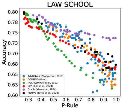
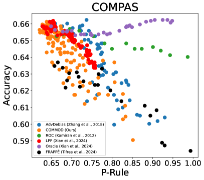
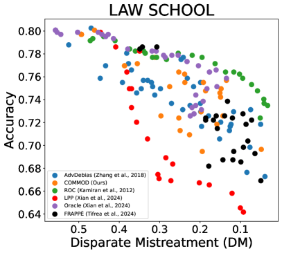
As traditionally done for bias mitigation methods, we evaluate the efficacy of COMMOD to preserve accuracy when enforcing fairness through the so-called Pareto plot. Figure 7 shows the accuracy and fairness scores achieved by all methods on Law School and Compas datasets (each dot represents one run). In terms of direct competitors, we observe that COMMOD outperforms LPP (resp. FRAPPE) on the Law School dataset (resp. Compas) and achieves similar results in the Compas dataset (resp. Law School). Further, we show here that even by adding the Minimal Changes and Interpretability constraints in Equation 4 COMMOD achieves almost similar results on all datasets as the in-processing method AdvDebias. Finally, as expected, Oracle (and also by ROC in Compas) generally outperform all methods. Hence, COMMOD remains a competitive algorithm in terms of fairness and accuracy, regardless of its other benefits, addressed in the next sections.
E.3 Intuition behind linear self-explainable model.
One might question why we chose to introduce explainability into our method through a linear architecture that learns concepts as linear combinations of the input features. Typically, using a linear model instead of a more complex one can lead to a decrease in model performance. However, the rationale behind our choice is clarified through the following experiment, where we evaluate different architectures for the network that learns the multiplicative ratio.
From the plot above, we can observe that the linear architecture performs similarly to more complex models. This observation aligns with the findings in Ţifrea et al. (2023), where a similar conclusion was drawn regarding their additive term, which is conceptually similar to our multiplicative ratio. Based on these insights, we decided to design the architecture of the ratio as a one-hidden-layer linear network. In this design, the hidden layer acts as a bottleneck that represents the concepts, and the output layer computes the ratio as a linear combination of these concepts.
Additionally, maintaining linearity between the concepts and the output ratio allows us to easily determine the direction (positive or negative) in which each concept influences the ratio’s value. This design choice enhances both the interpretability and transparency of the model.
E.4 Benefits of MSE Loss
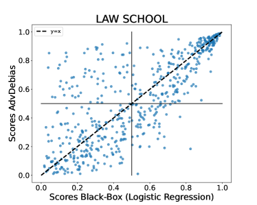
In this section, we propose a visualization in support to the MSE loss we chose to keep as similar as possible the edited scores with the ones outputted by the black-box algorithm. To do so, we used a "calibration" plot on edited scores vs black-box scores for our COMMOD algorithm and for AdvDebias for similar levels of . From such a plot, one can observe that the curve of COMMOD is more stick to the dashed line, representing when probabilities are not changed at all by the editing. On the other hand, we observe that in even if we do not change a prediction label, the probabilities are more scattered in the area of the dashed line. This behavior is beneficial for our motivation. When you want to edit a model for fairness, you usually want to do changes that flip labels (and hence that modifies the values of your fairness definition) and keep the other instances at the same confidence they were before.
E.5 Posthoc vs self explainable
As a final experiment, we aim to demonstrate the need for an approach specifically designed for Controlled Model Debiasing such as COMMOD. For this purpose, we build on the previous experiment and show that the combination of FRAPPE (which minimizes the number of changes) and a post-hoc interpretability tool leads to less efficient models in terms of debiasing; in other words, that adding interpretability in a post-hoc way comes at a higher cost for fairness. We train FRAPPE and COMMOD on the Law School dataset such that their scores in terms of accuracy, fairness and number of changes are comparable. We then train a decision tree to model FRAPPE’s additive output, and show in Figure 10 the final P-Rule obtained by COMMOD and this built competitor. We observe that, regardless of the tree’s depth, controlling the debiasing by introducing interpretability in a post-hoc way heavily degrades fairness, contrary to COMMOD.