Short-rate Derivatives in a Higher-for-Longer Environment
Abstract
We introduce a class of short-rate models that exhibit a “higher for longer” phenomenon. Specifically, the short-rate is modeled as a general time-homogeneous one-factor Markov diffusion on a finite interval. The lower endpoint is assumed to be regular, exit or natural according to boundary classification while the upper endpoint is assumed to be regular with absorbing behavior. In this setting, we give an explicit expression for price of a zero-coupon bond (as well as more general interest rate derivatives) in terms of the transition density of the short-rate under a new probability measure, and the solution of a non-linear ordinary differential equation (ODE). We then narrow our focus to a class of models for which the transition density and ODE can be solved explicitly. For models within this class, we provide conditions under which the lower endpoint is regular, exit and natural. Finally, we study two specific models – one in which the lower endpoint is exit and another in which the lower endpoint is natural. In these two models, we give an explicit solution of transition density of the short-rate as a (generalized) eigenfunction expansion. We provide plots of the transition density, (generalized) eigenfunctions, bond prices and the associated yield curve.
Keywords: short-rate model, interest rate, bond pricing, yield curve, spectral methods
1 Introduction
Between January of 2021 to December of 2021, the annual rate of inflation in the United States rose from 1.4% to 7.0% (source: BLS ).
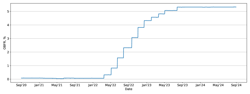
Although Treasury Secretary Janet Yellin initially called the rapid rise in inflation “transitory,” it had become apparent by early 2022 that high levels of inflation had become entrenched. In an effort get inflation down to its 2% target, between February of 2022 and August of 2023, the Federal Reserve raised its effective rate from roughly 0.1% to just over 5.3% (source: St. Louis Fed ). Despite the historically fast pace of interest rate hikes, the annual rate of inflation in September of 2023 was still sitting at 3.7%, leading Federal Reserve Chairman Jerome Powell to declare that interest rates would likely remain “higher for longer.” And, indeed, after topping out 5.32% in July of 2023, the federal overnight rate remained at this value until August of 2024.
In this paper, we present a class of one-factor short-rate models that capture this “higher for longer” phenomenon. Specifically, we assume that the short-rate is modeled as a Markov diffusion on a finite interval. The upper end of the interval is a regular (i.e., accessible) boundary according the Feller’s boundary classification, and is assumed to have absorbing behavior. That is, when the short rate reaches the upper end of the interval, it remains there forever. Although in reality, the federal reserve will likely lower interest rates when inflation returns to the Federal Reserve’s 2% target, the absorbing behavior captures the effect of interest rates remaining high for an extended period of time. Thus, the class of models in this paper can be seen as valid up to some finite time-horizon, after which the short-rate may be lowered. The class of models in this paper has the additional benefit of being analytically tractable, as the bond price can be written explicitly.
The rest of this paper proceeds as follows:
in Section 2 we introduce a class of short-rate models described by a one-factor Markov diffusion on a finite interval.
In this setting, we use risk-neutral pricing to derive an expression for the value of a financial derivative whose payoff depends on the terminal value of the short-rate.
We additionally relate the value of this financial derivative to the solution of a partial differential equation (PDE).
In Section 3, we perform a change of variables that enables us to express the solution of the pricing PDE in terms of the solutions of a nonlinear ordinary differential equation (ODE) and generalized eigenvalue problem.
Lastly, in Section 4, we consider a class of short-rate models for which the ODE and generalized eigenvalue problem described in Section 3 can be solved explicitly. We additionally perform a numerical study of bond prices and the resulting yield curves for two specific examples within this class. The two examples are qualitatively different in that the first example has an exit boundary at the origin and the eigenvalue problem has a discrete set of solutions, while the second example has a natural boundary at the origin and the eigenvalue problems has a continuous set of solutions.
2 Short-rate model and Pricing
To begin, we fix a time horizon and consider a continuous-time financial market, defined on a filtered probability space with no arbitrage and no transaction costs. The probability measure represents the market’s chosen pricing measure taking the money market account as numéraire. The filtration represents the history of the market.
We suppose that the money market account is strictly positive, continuous and non-decreasing. As such, there exists a non-negative -adapted short-rate process such that
| (1) |
We will focus on the case in which the dynamics of the short-rate are described by a Stochastic Differential Equation (SDE) of the following form
| (2) |
where is a -Brownian motion. We assume that the drift and volatility are such that the origin is either a regular, exit or a natural boundary, and that is a regular boundary, according to Feller’s boundary classification for scalar diffusions Feller [1952].
We further assume that has a unique strong solution up until the first exit time of . Observe that, as soon as exits , we have due to the indicator function on the right-hand side of (2). And thus, the endpoint is an absorbing state if it is a regular or exit boundary and endpoint is an absorbing state.
Let us denote by the value of a financial derivative that has a payoff at time , where . Using standard risk-neutral pricing, we have
| (3) |
Solving for and using and , we obtain
| (4) |
where we have used the Markov property of to express as a function of . By the Feynman-Kac formula, the function satisfies the following partial differential equation (PDE) and boundary conditions (BCs)
| (5) | |||||
| (6) | |||||
| (7) | |||||
where the operator is the infinitesimal generator of under and is given explicitly by
| (8) |
Throughout this paper we assume that Cauchy problem (5)-(7) has a unique classical solution.
Notice that the function defined in (4) depends on the maturity date and the payoff function . If we wish to emphasize the dependence of on and , we may sometimes write . For example, denoting by the price of a zero-coupon bond that pays one unit of currency at the maturity date and by the associated yield to maturity, we have
| (9) |
3 Solving the pricing PDE
In this section, we will obtain an explicit expression for the solution of Cauchy problem (5)-(7). The expression we obtain will depend on the solution of a first order, nonlinear, ordinary differential equation (ODE) as well as the (possibly improper) eigenfunctions and eigenvalues of a linear second-order differential operator. We begin with a short lemma.
Lemma 1.
Let be the unique classical solution of Cauchy problem (5)-(7). Suppose satisfies the following ordinary differential equation
| (10) |
where the operator is given by (8). Define the function as follows
| (11) |
Then the function satisfies the following Cauchy problem
| (12) | |||||
| (13) | |||||
| (14) | |||||
where the operator and the function are given by
| (15) |
Proof.
At this point, it will be convenient to introduce the fundamental solution associated with the operator . Specifically, for any we define as the unique classical solution of
| (23) | |||||
| (24) | |||||
| (25) | |||||
Remark 2.
Consider the following change of measure
| (26) |
We have from Girsanov’s Theorem that the process , defined by
| (27) |
is a -Brownian motion. From (2) and (27), we see that the dynamics of under are
| (28) |
and the generator of under is the operator given in (15). If follows that the solution of (23)-(25) is the transition density of under .
We can now state the main result of this section.
Theorem 3.
Proof.
Observe from (31) that, to write the solution of (5)-(7), we need an expression for a solution of (10). The following Proposition gives sufficient conditions on the coefficients and under which (10) has an explicit solution.
Proposition 4.
Suppose and are given by
| (32) |
for some non-negative function . Then
| (33) |
is a solution of (10), where is an arbitrary constant.
Proof.
We note from (31) that, to write the solution of (5)-(7), we need an expression for the solution of (23)-(25). To this end, it will be helpful to write the operator in self-adjoint form. We have
| (35) |
where we have introduced the scale density and the speed density of the operator . The scale and speed densities will be needed later in this paper to determine the behavior of the short-rate at the origin.
Assumption 5.
Henceforth, we assume the spectrum of , denoted , is simple.
Now, consider the following eigenvalue problem
| (36) | |||||
| (37) | |||||
| (38) | |||||
In general, the spectrum of self-adjoint operator has the decomposition , where and denote the discrete and continuous portions of , respectively. We will denote by the set of proper eigenvalues of and by the set of improper eigenvalues of . Similarly, we will denote by the proper eigenfunctions of , normalized as follows
| (39) |
and by the improper eigenfunctions of , normalized according to
| (40) |
where for some . Then, under Assumption 5, we have from [Hanson and Yakovlev, 2013, Chapter 5] that the solution of (23)-(25) has the following (generalized) eigenfunction representation
| (41) |
Thus, we need only to solve eigenvalue problem (36)-(38) to construct the transition density . The following proposition, which is based on the transformation to Liouville normal form [DLMF, , Chapter 1], can be helpful to find solutions of the eigenvalue equation (36) in the case where and are given by (32) for some non-negative function .
Proposition 6.
Let be a non-negative function. Suppose and are given by (32). Then the scale density , the speed density , defined in (35), are given by
| (42) |
where is an arbitrary constant, and the operator is given by
| (43) |
Suppose is a (possibly improper) eigenfunction of , which satisfies (36)-(38). Define functions and through the following equations
| (44) |
Then satisfies
| (45) | ||||||||
| (46) | ||||||||
| (47) | ||||||||
where is the inverse of .
4 A class of analytically tractable models
In this section, we analyze a class of models for the short rate in which the drift and volatility are given by (32) with the function being given by
| (49) |
Inserting (49) into (32) we obtain
| (50) |
Thus, we have from (2) and (50) that the dynamics of the short-rate are given by
| (51) |
Remark 7.
corresponds to a geometric Brownian motion with and .
It then follows from (43) that the operator is given by
| (52) |
and from (42) the scale density and the speed density are given by
| (53) | ||||
| (54) |
In order to write spectral representation of the transition density (41) for the short-rate (51), we must determine the structure of the spectrum of the diffusion generator (52), which depends on whether the origin is regular, exit or natural. This will also determine if a BC (24) is needed at the origin.
Proposition 8.
Fix an interval and consider the operator given by (52). For the origin is natural, for the origin is exit, and for the origin is regular.
Proof.
See Appendix A. ∎
Using (44) and (45) we have for that
| (55) |
and for we have
| (56) |
Thus, from (45), (46) and (47), we have for that satisfy
| (57) | |||||
| (58) | |||||
| (59) | |||||
For the origin is a natural boundary by Proposition 8. Hence, we have
| (60) | ||||
| (61) |
Notice that when , after the Liouville transformation as in (55) and (56), the origin turns into , which plays a role in the following decomposition of spectrum .
Proposition 9.
Fix an interval and consider the operator given by (52). For the spectrum is purely discrete, i.e. , for the spectrum is purely continuous , and for the spectrum is mixed, with discrete portion clustering at and continuous portion .
Proof.
Notice that the right endpoint is always regular. By Proposition 8 in case the origin is either exit or regular. According to Linetsky [2007] regular and exit boundaries are always non-oscillatory. Therefore, both endpoints in this case are non-oscillatory and the operator is of the spectral category I (i.e., its spectrum is purely discrete and lies in ).
For , the origin is natural by Proposition 8. From (55) and (56) we have
| (62) |
i.e., the origin is transformed into by Liouville transformation (44). Then, we investigate the potential in (55) and (56). We have
| (63) |
As this limit is finite, the origin is an oscillatory boundary with cutoff . This, together with being regular and thus non-oscillatory, implies that the operator is of the spectral category II. Therefore for () it has purely continuous spectrum in , while for () it has continuous spectrum and discrete spectrum in clustering at . ∎
For certain choices of , we can express , the solution of (57) corresponding to eigenvalue in terms of special functions. We provide some examples here
| (64) | ||||||
| (65) | ||||||
| (66) | ||||||
| (67) | ||||||
| (68) | ||||||
where is the Tricomi’s confluent hypergeometric function, is the generalized Laguerre polynomial, is the double-confluent Heun function [Wolfram, , HeunD function], and are Bessel functions, and is the modified Bessel function of the first kind. The constants and are chosen to satisfy the BCs (46), (47) and (61) together with normalization (39) or (40) for (44) with respect to where is the speed density given by (42).
4.1 Example: , the origin is exit
For , the SDE (51) of the short-rate becomes
| (69) |
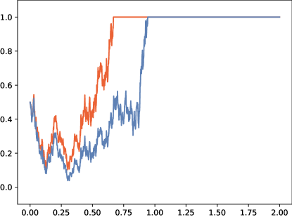
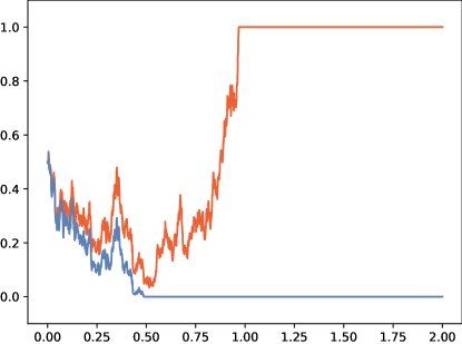
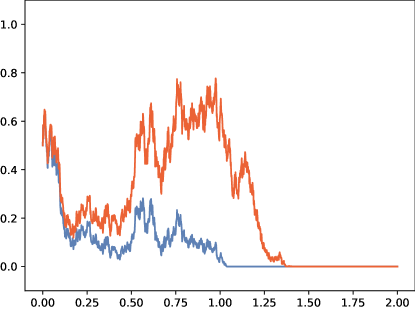
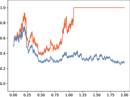
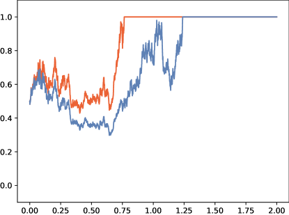
In Figure 2, using a standard Euler-Maruyama method, we plot four sample trajectories of the short-rate (69) under (corresponding to generator in (8)) as well as the corresponding trajectories of the short-rate under (corresponding to generator in (52)). As the origin is exit and is regular, the short-rate can hit both endpoints and . However, the trajectories spend more time near the origin than they do near before reaching either due to the fact that as .
Proposition 10.
For (dynamics of given by (69)) the origin is exit, the spectrum is purely discrete and the eigenfunctions (36), normalized as (39), have the following form
| (70) | ||||
| (71) |
where is a Kummer’s confluent hypergeometric function, that is [DLMF, , Chapter 13]
| (72) |
while the eigenvalues are solutions of
| (73) |
Then, the transition density (23) admits the representation
| (74) |
Proof.
See Appendix B ∎
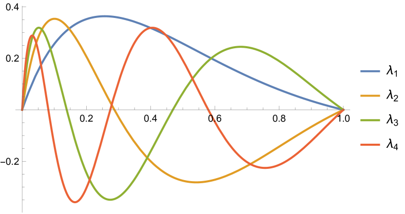
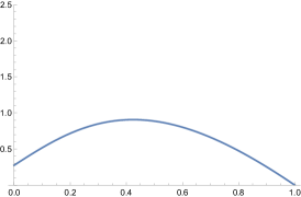
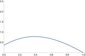
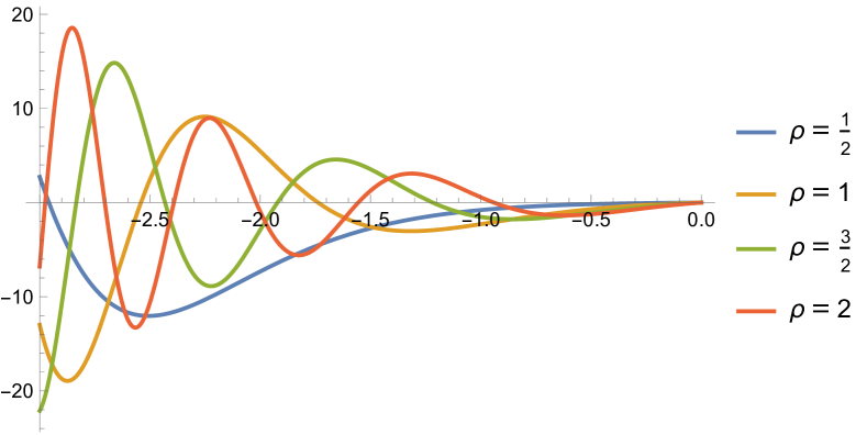
In Figure 3, with , we plot the first four normalized eigenfunctions (70), corresponding to . Smaller is associated with a more oscillatory eigenfunction.
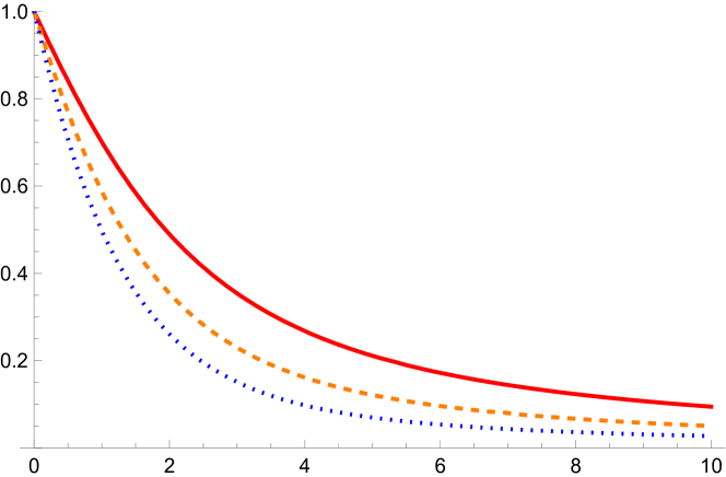
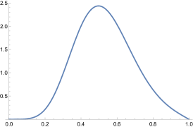
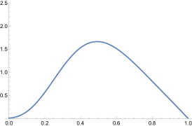
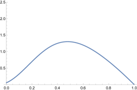
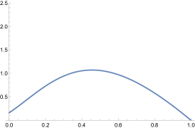
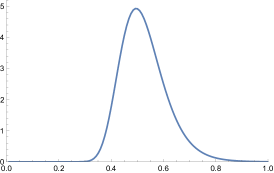
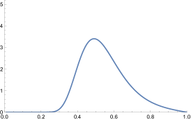
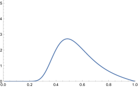
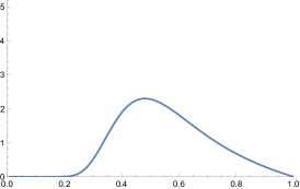
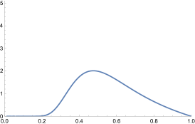
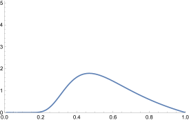
In Figure 4, we plot the transition density (74) as a function of with and fixed, and going from to in steps of . The area under the density curve is less than for because has a positive probability of being located at one of the endpoints.
Remark 11.
To compute bond prices (and the prices of other financial derivatives), we must compute an expression for (33). From (49) we have
| (76) |
Proposition 12.
Proof.
4.2 Example: , the origin is natural
For , the SDE (51) of the short-rate becomes
| (83) |
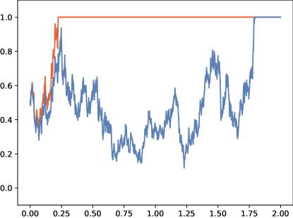
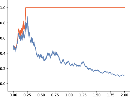
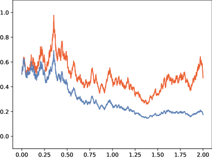
In Figure 7, with , we plot sample trajectories of the short-rate (83) under (corresponding to generator in (8)) as well as the corresponding trajectories for the short-rate under (corresponding to generator in (52)). Note that the short-rate can hit the right endpoint , which is regular, while it cannot reach the origin, which is natural.
Proposition 13.
For model (83) the origin is natural, the spectrum of (52) is purely continuous in and the improper eigenfunctions (36) normalized as (40) have the following form
| (84) |
where is the Bessel function of the first kind and is the modified Bessel function of the second kind. Then, the transition density (23) admits the representation
| (85) |
Proof.
See Appendix D. ∎
Remark 14.
Remark 15.
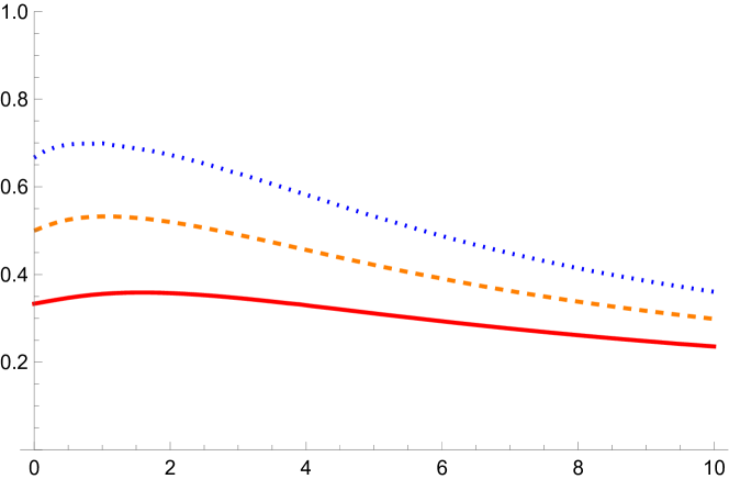
In Figure 8, with we plot four improper normalized eigenfunctions (84), where we use the natural log scale for the axis. Notice that as eigenfunctions exhibit highly oscillatory behavior. In Figure 9 we plot the transition density (85) as a function of with and fixed, and ranging from to with step . The transition density goes to in the neighborhood of the origin, as expected due to the origin being natural. The area under the density curve is less than for , because there is positive probability that , which is regular endpoint.
Proposition 16.
Proof.
Acknowledgments
Aram Karakhanyan acknowledges partial support from EPSRC grant EP/S03157X/1 Mean curvature measure of free boundary.
Appendix A Proof of Proposition 8
Consider the scale measure
| (95) |
where is a scale density (53), together with the limiting case at the origin
| (96) |
The boundary classification of the origin depends on the following integrals
| (97) | ||||
| (98) |
where and is a speed density (54). In particular, according to Linetsky [2007], the origin is
-
1.
regular if and ,
-
2.
exit if and ,
-
3.
natural if and .
Thus, in order to classify the origin, it is sufficient to determine whether each of the integrals and converges or diverges.
For simplicity, denote
| (99) |
then evaluating (95) we get the expression for the scale measure
| (100) |
Next, we compute as in (96)
| (101) |
Then by plugging (54) and (101) into (97) for we get
| (102) |
Using the asymptotic equivalence
| (103) |
it follows that convergence of coincides with convergence of
| (104) |
but the latter integral converges for and diverges for . Together with (101) for this results in
| (105) |
Plugging (54) and (100) into (98) for
| (106) |
Notice that since as for , and for , so we have asymptotic equivalence
| (107) |
where
| (108) |
Thus convergence of (98) coincides with convergence of
| (109) |
which converges for , so in this case, and diverges for , so . For
| (110) |
from asymptotic equivalence
| (111) |
Thus, we get
| (112) |
This, combined with (105) proves the proposition.
Appendix B Proof of Proposition 10
From Proposition 8 the origin is an exit boundary, and from Proposition 9 the spectrum is purely discrete. Plugging into (50), (53), (54) with , and (55) we get
| (113) |
Thus, from (57) and (113) we derive the following equation
| (114) |
Applying the first BC to the analytic solution (64) we get that , and expanding , the expression for the eigenfunctions becomes
| (115) |
where is a constant coefficient. Before applying the second BC, we return back to the original variable by plugging (113) and (115), into (44), resulting in
| (116) |
and using the Kummer’s transformation
| (117) |
(116) becomes
| (118) |
Now, applying the second BC (38)
| (119) |
Thus, the eigenvalues are solutions of this equation, or of (73) equivalently. The constant for each is determined from normalization (39) with (113).
| (120) |
so if we introduce (71), then
| (121) |
which produces (70). Finally, since the spectrum is purely discrete, i.e. and , the expression for the transition density (74) follows from the general spectral representation (41).
Appendix C Spectral representation for the natural boundary case
In practice, when the origin is natural and, consequently, the continuous spectrum is nonempty (see Proposition 9), the eigenfunction representation is written by finding the Green’s function first [Borodin and Salminen, 2002, Chapter 2]
| (122) |
where and are solutions of (36) s.t. is increasing, while is decreasing and satisfies (38). Both functions should satisfy some additional conditions at the origin to ensure Green’s function uniqueness, that is
| (123) | ||||||
| (124) |
where is defined as in (96). These conditions will typically be satisfied for and under the prior assumptions, but when they are not, one must change and accordingly. Under the aforementioned conditions on and , the Wronskian (122) will be independent of which justifies the notation.
Then, applying inverse Laplace transform to (122) results in
| (125) |
which produces a discrete part of (41) when the Green’s function has isolated singularities, and a continuous part when there is a branch cut for .
Appendix D Proof of Proposition 13
From Proposition 8 the origin is a natural boundary, and from Proposition 9 the spectrum is purely continuous in . Plugging into (50), (53), (54) with , and (55) we get
| (126) |
From (57) we derive the following equation
| (127) |
The general solution to this ODE is given by (68). First, we return back to the original variable by plugging (68) and (126) (44). This results in the general solution of the eigenvalue equation (36)
| (128) |
where are the Bessel functions. (128) is a linear combination of two independent solutions
| (129) |
Following the approach described in Appendix C, we need to construct two solutions and of (36) s.t. for is increasing, while is decreasing and satisfies the BC (38)
| (130) | ||||
| (131) | ||||
| (132) |
where are the modified Bessel functions, and we have used the following connection formulas between regular and modified Bessel functions [DLMF, , Chapter 10] which hold for all
| (133) |
Plugging (126), (130) and (132) into the Wronskian (122) results in
| (134) |
Plugging (130), (132) and (134) into (122) we compute the Green’s function
| (135) | ||||
| (136) |
Finally, to get the transition density, we must invert the Laplace transform (125) with (126). Since and has no poles, we close the contour in the left half-plane and apply the Jordan’s lemma. Then, using the substitution to account for the branch cut, we get
| (137) |
the integrand can be simplified as
| (138) | ||||
| (139) | ||||
| (140) |
plugging this into (137) and introducing (84) results in (85). Finally, we notice that (84) satisfy
| (141) |
which is (36) for (52) with , and since
| (142) |
satisfy (38). Therefore are indeed improper eigenfunctions, and from the uniqueness of spectral representation (41) we conclude that they satisfy the normalization (40).
References
- [1] BLS. US Bureau of Labor Statistics. https://data.bls.gov/timeseries/CUUR0000SA0?output_view=pct_12mths. Accessed: 2025-01-20.
- Borodin and Salminen [2002] A. Borodin and P. Salminen. Handbook of Brownian Motion - Facts and Formulae. Probability and Its Applications. Birkhäuser Basel, 2002. ISBN 978-3-7643-67053. doi: 10.1007/978-3-0348-8163-0.
- [3] DLMF. NIST Digital Library of Mathematical Functions. https://dlmf.nist.gov/, Release 1.2.1 of 2024-06-15. URL https://dlmf.nist.gov/. F. W. J. Olver, A. B. Olde Daalhuis, D. W. Lozier, B. I. Schneider, R. F. Boisvert, C. W. Clark, B. R. Miller, B. V. Saunders, H. S. Cohl, and M. A. McClain, eds.
- Feller [1952] W. Feller. The parabolic differential equations and the associated semi-groups of transformations. Annals of Mathematics, 55:468–519, 1952. URL https://api.semanticscholar.org/CorpusID:123972208.
- Hanson and Yakovlev [2013] G. W. Hanson and A. B. Yakovlev. Operator Theory for Electromagnetics: An Introduction. Springer New York, NY, 2013. ISBN 978-0-387-95278-9. doi: 10.1007/978-1-4757-3679-3.
- Linetsky [2007] V. Linetsky. Chapter 6 spectral methods in derivatives pricing. In J. R. Birge and V. Linetsky, editors, Financial Engineering, volume 15 of Handbooks in Operations Research and Management Science, pages 223 – 299. Elsevier, 2007.
- [7] St. Louis Fed. Federal Reserve Bank of St. Louis. https://fred.stlouisfed.org/series/FEDFUNDS. Accessed: 2025-01-20.
- [8] Wolfram. Wolfram Language and System Documentation Center. https://reference.wolfram.com/language/ref/HeunD. Accessed: 2025-01-24.
Figures
https://www.newyorkfed.org/markets/reference-rates/obfr
 |
 |
 |
 |
 |
 |
 |
 |
 |
 |
 |
 |
 |
 |
 |
 |
 |
 |
 |
 |