Dynamics of the NLS-log equation on a tadpole graph

Jaime Angulo Pava and Andrés Gerardo Pérez Yépez 1
Abstract

This work aims to study some dynamics issues of the nonlinear logarithmic Schrödinger equation (NLS-log) on a tadpole graph, namely, a graph consisting of a circle with a half-line attached at a single vertex. By considering $\delta$-type boundary conditions at the junction we show the existence and the orbital stability of standing-waves solutions with a profile determined by a positive single-lobe state. Via a splitting eigenvalue method, we identify the Morse index and the nullity index of a specific linearized operator around an a priori positive single-lobe state. To our knowledge, the results contained in this paper are the first in studying the (NLS-log) on tadpole graphs. In particular, our approach has the prospect of being extended to study stability properties of other bound states for the (NLS-log) on a tadpole graph or another non-compact metric graph such as a looping edge graph.

1 Department of Mathematics, IME-USP

Rua do Matão 1010, Cidade Universitária, CEP 05508-090, São Paulo, SP, Brazil.

andresgerardo329@gmail.com

angulo@ime.usp.br

Mathematics Subject Classification (2020). Primary 35Q51, 35Q55, 81Q35, 35R02; Secondary 47E05.
Key words. Nonlinear Schrödinger model, quantum graphs, standing wave solutions, stability, extension theory of symmetric operators, Sturm Comparison Theorem.

1 Introduction

The following Schrödinger model with a logarithmic non-linearity (NLS-log)

$$i\partial_{t}u+\Delta u+uLog|u|^{2}=0,$$ (1.1)

where $u=u(x,t):\,\mathbb{R}^{N}\times\mathbb{R}\rightarrow\mathbb{C}$, $N\geq 1$, was introduced in 1976 by Bialynicki-Birula and Mycielski [17] built a model of nonlinear wave mechanics to obtain a nonlinear equation which helped to quantify departures from the strictly linear regime, preserving in any number of dimensions some fundamental aspects of quantum mechanics, such as separability and additivity of total energy of noninteracting subsystems. The NLS model in (1.1) equation admits applications to dissipative systems [30], quantum mechanics, quantum optics [18], nuclear physics [29], transport and diffusion phenomena (for example, magma transport) [24], open quantum systems, effective quantum gravity, theory of superfluidity and Bose-Einstein condensation (see [29, 39] and the references therein).

The NLS-log ($N=1$) on some metric graphs was studied by several authors in the last years (see [8, 10, 11, 14, 15] and reference therein). Two basic metric graphs $G_{i}$, $i=0,1$, were considered by many authors, for $G_{0}=(-\infty,0)\cup(0,+\infty)$ with boundary $\delta$-or $\delta^{\prime}$-interactions at the vertex $\nu=0$ were obtained the existence and orbital (in)stability of standing waves solutions with a Gausson profile. A similar study was also considered for $G_{1}=\bigcup_{j=1}^{N}(0,+\infty)$, the so-called a star metric graph with the common vertex $\nu=0$.

In this work, we are interested in studying some issues associated with the existence and orbital stability of standing waves solutions of the NLS-log ($N=1$) on a tadpole graph, namely, the following vectorial model

$$i\partial_{t}\mathbb{U}+\Delta\mathbb{U}+\mathbb{U}Log|\mathbb{U}|^{2}=0.$$ (1.2)

on a graph given by a ring with one half-line attached at one vertex point (see Figure 1 below).

Refer to caption
Figure 1: Tadpole graph

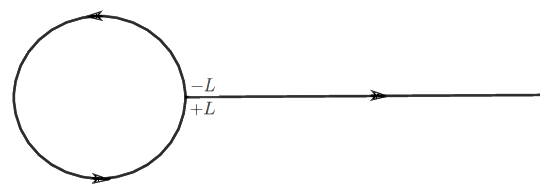
Thus, if in the tadpole graph, the ring is identified by the interval $[-L,L]$ and the semi-infinite line with $[L,+\infty)$, we obtain a metric graph $\mathcal{G}$ with a structure represented by the set $\mathbb{E}=\{e_{0},e_{1}\}$ where $e_{0}=[-L,L]$ and $e_{1}=[L,+\infty)$, which are the edges of $\mathcal{G}$ and they are connected at the unique vertex $v=L$. $\mathcal{G}$ is also called a lasso graph (see [25] and references therein). In this form, we identify any function $U$ on $\mathcal{G}$ (the wave functions) with a collection $U=(u_{e})_{e\in E}$ of functions $u_{e}$ defined on the edge $e$ of $\mathcal{G}$. In the case of the NLS-log in (1.2), we have $U(x_{e},t)=(u_{e}(x_{e},t))_{e\in\mathbb{E}}$ and the nonlinearity $ULog|U|^{2}$, acting componentwise, i.e., for instance $(ULog|U|^{2})_{e}=u_{e}Log|u_{e}|^{2}$. The action of the Laplacian operator $\Delta$ on the tadpole $\mathcal{G}$ is given by

$$-\Delta:(u_{e})_{e\in E}\rightarrow(-u^{\prime\prime}_{e})_{e\in\mathbb{E}}.$$ (1.3)

Several domains make the Laplacian operator to be self-adjoint on a tadpole graph (see Angulo&Mun$\bar{o}$z [12] and Exner et al. [25, 26, 27]). Here, we will consider a domain of general interest in physical applications. In fact, if we denote a wave function $U$ on the tadpole graph $\mathcal{G}$ as $U=(\Phi,\Psi)$, with $\Phi:[-L,L]\rightarrow\mathbb{C}$ and $\Psi:[L,\infty)\rightarrow\mathbb{C}$, we define the following domains for $-\Delta$:

$$D_{Z}=\{U\in H^{2}(\mathcal{G}):\Phi(L)=\Phi(-L)=\Psi(L),\text{ and, }\Phi^{\prime}(L)-\Phi^{\prime}(-L)=\Psi^{\prime}(L+)+Z\Psi(L)\},$$ (1.4)

with $Z\in\mathbb{R}$ and for any $n\geq 0$, $n\in\mathbb{N}$,

$$H^{n}(\mathcal{G})=H^{n}(-L,L)\oplus H^{n}(-L,+\infty).$$

The boundary conditions in (1.4) are called of $\delta$-interaction type if $Z\neq 0$, and of flux-balanced or Neuman-Kirchhoff condition if $Z=0$ (with always continuity at the vertex). It is not difficult to see that $(-\Delta,D_{Z})_{Z\in\mathbb{R}}$ represents a one-parameter family of self-adjoint operators on the tadpole graph $\mathcal{G}$. We note that is possible to determine other domains where the Laplacian is self-adjoint on a tadpole ($\Phi(L)=\Phi(-L)$), in fact, via the results in Angulo&Mun$\bar{o}$z [12] (see Example 9) we have domains that can be characterized by the following family of 6-parameters of boundary conditions

$$\begin{split}&\Phi(-L)=\Phi(L),\;\;(1-m_{3})\Phi(L)=m_{4}\Psi(L)+m_{5}\Psi^{\prime}(L),\\ &\Phi^{\prime}(L)-2\Phi^{\prime}(-L)=m_{1}\Phi(-L)+A_{1}\Psi(L)+A_{2}\Psi^{\prime}(L)\ \mbox{and }\\ &\Phi^{\prime}(L)-A_{3}\Psi^{\prime}(L)=m_{6}\Phi(-L)+m_{7}\Psi(L),\end{split}$$ (1.5)

$A_{1}=m_{4}m_{6}-m_{3}m_{7}$, $A_{2}=m_{5}m_{6}-\frac{2m_{3}+m_{7}m_{5}m_{3}}{m_{4}}$ and $A_{3}=\frac{2+m_{7}m_{5}}{m_{4}}$, $m_{1},m_{3},m_{4},m_{5},m_{6},m_{7}\in\mathbb{R}$ and $m_{4}\neq 0$. Note that for $m_{3}=m_{5}=0$ and $m_{4}=1$, we get the so-called $\delta$-interaction conditions in (1.4). Moreover, for $m_{1}=m_{6}=m_{7}=0$, $m_{3}=1$, $m_{4}=2$, and $m_{5}$ arbitrary, we get the following $\delta^{\prime}$-interaction type condition on a tadpole graph

$$\begin{split}&\Phi^{\prime}(-L)=\Phi^{\prime}(L)=\Psi^{\prime}(L),\;\;\Phi(L)=\Phi(-L)\;\;\mbox{and}\\ &\Psi(L)=-\frac{m_{5}}{2}\Psi^{\prime}(L).\end{split}$$ (1.6)

Our main interest here will be to study some dynamics issues for (1.2) such as the existence and orbital stability of standing waves solutions given by the profiles $U(x,t)=e^{ict}\Theta(x)$, with $c\in\mathbb{R}$, $\Theta=(\phi,\psi)\in D_{Z}$ (real-valued components), and satisfying the NLS-log vectorial equation

$$-\Delta\Theta+c\Theta-\Theta Log(\Theta^{2})=0.$$ (1.7)

More explicitly $\phi$ and $\psi$ satisfy the following system, one on the ring and the other one on the half-line respectively,

$$\left\{\begin{array}[]{ll}-\phi^{\prime\prime}(x)+c\phi(x)-log(\phi^{2}(x))\phi(x)=0,\;\;\;\;x\in(-L,L),\\ -\psi^{\prime\prime}(x)+c\psi(x)-log(\psi^{2}(x))\psi(x)=0,\;\;\;\;x\in(L,+\infty),\\ \phi(L)=\phi(-L)=\psi(L),\\ \phi^{\prime}(L)-\phi^{\prime}(-L)=\psi^{\prime}(L+)+Z\psi(L),\;\;\;\;Z\in\mathbb{R}.\end{array}\right.$$ (1.8)

It is clear that the delicate point in the existence of solutions for (1.8) is given for the component $\phi$ on $[-L,L]$ and satisfying the $\delta$-coupling condition. The component of $\psi$ will be obviously a translated Gausson-profile (see [9]) in the form

$$\psi_{c}(x)=e^{\frac{c+1}{2}}e^{\frac{-(x-L+a)^{2}}{2}},\ \ \ a\neq 0,\ \ \ c\in\mathbb{R},\ \ \ x\geq L.$$ (1.9)

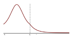
Among all profiles for (1.8), we are interested here in the positive single-lobe states. More precisely, we have the following definition (see Figure 2).

Definition 1.1.

The profile standing wave $\Theta=(\phi,\psi)\in D_{Z}$, is said to be a positive single-lobe state for (1.8) if every component is positive on each edge of $\mathcal{G}$, the maximum of $\Theta$ is achieved at a single internal point, symmetric on $[-L,L]$ , and monotonically decreasing on $[0,L]$. Moreover, $\psi$ is strictly decreasing on $[L,+\infty)$.

Refer to caption
Figure 2: A positive single-lobe state profile for the NLS-log model on $\mathcal{G}$

The study of either ground or bound states on general metric graphs for the NLS model with a polynomial nonlinearity

$$i\partial_{t}\mathbb{U}+\Delta\mathbb{U}+|\mathbb{U}|^{2p}\mathbb{U}=0,\quad p>0$$ (1.10)

has been studied in [7, 6, 1, 2, 3, 19, 36, 31, 35]. To our knowledge, the results contained in this paper are the first in studying the NLS-log on tadpole graphs.

Our focus in this work is to study the existence and orbital stability for the NLS-log in the case $Z=0$ in (1.8), Neuman-Kirchhoff condition, that is, positive single-lobe states $\Theta=(\phi,\psi)\in D_{0}$. For the convenience of the reader, we establish the main points in the stability study of standing wave solutions for NLS-log models on a tadpole graph. After that, we give the main results of our work. So, by starting, we note that the basic symmetry associated to the NLS-log model (1.2) on tadpole graphs is the phase invariance, namely, if $\mathbf{U}$ is a solution of (1.2) then $e^{i\theta}\mathbf{U}$ is also a solution for any $\theta\in[0,2\pi)$. Thus, it is reasonable to define orbital stability for the model (1.2) as follows (see [28]) .

Definition 1.2.

The standing wave $\mathbf{U}(x,t)=e^{ict}(\mathbf{\phi}(x),\mathbf{\psi}(x))$ is said to be orbitally stable in a Banach space $X$ if for any $\varepsilon>0$ there exists $\eta>0$ with the following property: if $\mathbf{U}_{0}\in X$ satisfies $||\mathbf{U}_{0}-(\mathbf{\Phi},\mathbf{\Psi})||_{X}<\eta$, then the solution $\mathbf{U}(t)$ of (1.2) with $\mathbf{U}(0)=\mathbf{U}_{0}$ exists for any $t\in\mathbb{R}$ and

$$\sup\limits_{t\in\mathbb{R}}\inf\limits_{\theta\in[0,2\pi)}||\mathbf{U}(t)-e^{i\theta}(\mathbf{\phi},\mathbf{\psi})||_{X}<\varepsilon.$$

Otherwise, the standing wave $\mathbf{U}(x,t)=e^{ict}(\mathbf{\phi}(x),\mathbf{\psi}(x))$ is said to be orbitally unstable in $X$.

The space $X$ in Definition 1.2 for the model (1.2) will depend on the domain of action of $-\Delta$, namely, $D_{0}$, and a specific weighted space. Indeed, we will consider the following spaces

$$\mathcal{E}(\mathcal{G})=\left\{(f,g)\in H^{1}(\mathcal{G}):f(-L)=f(L)=g(L)\right\}\quad\text{``continuous energy-space''},$$ (1.11)

and the Banach spaces $W(\mathcal{G})$ and $\widetilde{W}$ defined by

$\displaystyle W(\mathcal{G})=\{(f,g)\in\mathcal{E}(\mathcal{G}):|g|^{2}Log|g|^{2}\in L^{1}(L,+\infty)\}$ (1.12)
$\displaystyle\widetilde{W}=\{(f,g)\in\mathcal{E}(\mathcal{G}):xg\in L^{2}(L,\infty)\}.$

We note that $\widetilde{W}\subset W(\mathcal{G})$ (see Lemma 2.1 below). Thus, due to our local study related to the stability problem (not variational type) we will consider $X=\widetilde{W}$ in Definition 1.2.

Next, we consider the following two functionals associated with (1.2)

$$E(\mathbf{U})=\|\nabla\mathbf{U}\|^{2}_{L^{2}(\mathcal{G})}-\int_{-L}^{L}|f_{1}|^{2}log(|f_{1}|^{2})dx-\int_{L}^{\infty}|f_{2}|^{2}log(|f_{2}|^{2})dx,\qquad(\text{energy})$$ (1.13)

and

$$Q(\mathbf{U})=\|\mathbf{U}\|^{2}_{L^{2}(\mathcal{G})},\qquad\qquad\qquad\qquad\qquad\qquad\qquad\;\;\;\quad\qquad\quad\;\;\;(\text{mass})$$ (1.14)

where $\mathbf{U}=(f_{1},f_{2})$. These functional satisfy $E,Q\in C^{1}(W(\mathcal{G}):\mathbb{R})$ (see [20] or Proposition 6.3 in [8]) and, at least formally, $E$ is conserved by the flow of (1.2). The use of the space $W(\mathcal{G})$ is because $E$ fails to be continuously differentiable on $\mathcal{E}(\mathcal{G})$ (a proof of this can be based on the ideas in [20]). Now, as our stability theory is based on the framework of Grillakis et al. [28], $E$ needs to be twice continuously differentiable at the profile $\Theta\in D_{0}$. To satisfy this condition we introduced the space $\widetilde{W}$. Moreover, this space naturally appears in the following study of the linearization of the action functional around of $\Theta$. We note that $E,Q\in C^{1}(\widetilde{W})$.

Now, for a fixed $c\in\mathbb{R}$, let $\mathbf{U}_{c}(x,t)=e^{ict}(\mathbf{\phi}_{c}(x),\mathbf{\psi}_{c}(x))$ be a standing wave solution for (1.2) with $(\phi_{c},\psi_{c})\in D_{0}$ being a positive single-lobe state. Then, for the action functional

$$\mathbf{S}(\mathbf{U})=E(\mathbf{U})-(c+1)Q(\mathbf{U}),\quad\quad\mathbf{U}\in\widetilde{W},$$ (1.15)

we have $\mathbf{S}^{\prime}(\phi_{c},\psi_{c})=\mathbf{0}$. Next, for $\mathbf{U}=\mathbf{U}_{1}+i\mathbf{U}_{2}$ and $\mathbf{W}=\mathbf{W}_{1}+i\mathbf{W}_{2}$, where the functions $\mathbf{U}_{j}$, $\mathbf{W}_{j}$, $j=1,2$, are real. The second variation of $\mathbf{S}$ in $(\phi_{c},\psi_{c})$ is given by

$$\mathbf{S}^{\prime\prime}(\phi_{c},\psi_{c})(\mathbf{U},\mathbf{W})=\langle\mathcal{L}_{+,Z}\mathbf{U}_{1},\mathbf{W}_{1}\rangle+\langle\mathcal{L}_{-,Z}\mathbf{U}_{2},\mathbf{W}_{2}\rangle,$$ (1.16)

where the two $2\times 2$-diagonal operators $\mathcal{L}_{1}$ and $\mathcal{L}_{2}$ are given for

$$\begin{array}[]{ll}&\mathcal{L}_{1}=diag\left(-\partial_{x}^{2}+(c-2)-Log|\phi_{c}|^{2},-\partial_{x}^{2}+(c-2)-Log|\psi_{c}|^{2}\right)\\ \\ &\mathcal{L}_{2}=diag\left(-\partial_{x}^{2}+c-Log|\phi_{c}|^{2},-\partial_{x}^{2}+c-Log|\psi_{c}|^{2}\right)\end{array}$$ (1.17)

We note that these two diagonal operators are self-adjoint with domain (see Theorem 3.1 below)

$$\mathcal{D}:=\{(f,g)\in D_{0}:x^{2}g\in L^{2}([L,\infty))\}.$$

We also see that since $(\phi_{c},\psi_{c})\in\mathcal{D}$ and satisfies system (1.8), $\mathcal{L}_{2}(\phi_{c},\psi_{c})^{t}=\mathbf{0}$ and so the kernel of $\mathcal{L}_{2}$ is non-trivial, moreover as $\langle\mathcal{L}_{1}(\phi_{c},\psi_{c})^{t},(\phi_{c},\psi_{c})^{t}\rangle<0$, the Morse index of $\mathcal{L}_{1}$, $n(\mathcal{L}_{1})$, satisfies $n(\mathcal{L}_{1})\geqq 1$. Next, from [28] we know that the Morse index and the nullity index of the operators $\mathcal{L}_{1}$ and $\mathcal{L}_{2}$ are a fundamental step in deciding about the orbital stability of standing wave solutions. For the case of the profile $(\mathbf{\phi}_{c},\mathbf{\psi}_{c})$ being a positive single-lobe state, our main results are the following:

Theorem 1.3.

It consider the self-adjoint operator $(\mathcal{L}_{1},\mathcal{D})$ in (1.17) determined by the positive single-lobe state $(\mathbf{\phi}_{c},\mathbf{\psi}_{c})$. Then,

  1. 1)

    Perron-Frobenius property: let $\beta_{0}<0$ be the smallest eigenvalue for $\mathcal{L}_{1}$ with associated eigenfunction $(f_{\beta_{0}},g_{\beta_{0}})$. Then, $f_{\beta_{0}}$ is positive and even on $[-L,L]$, and $g_{\beta_{0}}(x)>0$ with $x\in[L,+\infty)$,

  2. 2)

    $\beta_{0}$ is simple,

  3. 3)

    the Morse index of $\mathcal{L}_{1}$ is one,

  4. 4)

    The kernel associated to $\mathcal{L}_{1}$ on $\mathcal{D}$ is trivial.

Theorem 1.4.

It consider the self-adjoint operator $(\mathcal{L}_{2},\mathcal{D})$ in (1.17) determined by the positive single-lobe state $(\mathbf{\phi}_{c},\mathbf{\psi}_{c})$. Then,

  1. 1)

    the kernel of $\mathcal{L}_{2}$, $ker(\mathcal{L}_{2})$, satisfies $ker(\mathcal{L}_{2})=span\{(\mathbf{\phi}_{c},\mathbf{\psi}_{c})\}$.

  2. 2)

    $\mathcal{L}_{2}$ is a non-negative operator, $\mathcal{L}_{2}\geqq 0$.

The proof of Theorem 1.3 will be based in a splitting eigenvalue method applied to $\mathcal{L}_{1}:=diag(L_{0},L_{1})$ in (1.17) on tadpole graph (see Lemma 4.4). More exactly, we reduce the eigenvalue problem associated with $\mathcal{L}_{1}$ with domain $\mathcal{D}$ to two classes of eigenvalue problems, one with periodic boundary conditions on $[-L,L]$ for $L_{0}$ and the other one with Neumann boundary conditions on $=[L,+\infty)$ for $L_{1}$. Thus, by using tools of the extension theory of Krein&von Neumann for symmetric operators, the theory of real coupled self-adjoint boundary conditions on $[-L,L]$ and the Sturm Comparison Theorem, will imply our statements.

Our result of orbital stability is the following:

Theorem 1.5.

Consider $Z=0$ in (1.8). Then, there exists a $C^{1}$-mapping $c\in\mathbb{R}\rightarrow\Theta_{c}=(\phi_{c},\psi_{c})$ of positive single-lobe states on $\mathcal{G}$. Moreover, for $c\in\mathbb{R}$, the orbit

$$\{e^{i\theta}\Theta_{c}:\theta\in[0,2\pi)\}$$

is stable.

The proof of Theorems 1.3-1.4 are given in Section 4. The statement of the orbital stability follows from Theorems 1.3-1.4 and from the abstract stability framework established by Grillakis&Shatah&Strauss in [28]. By the convenience of the reader, we establish in Theorem 8.7 (Appendix) an adaptation of the abstract results in [28] to the case tadpole graphs. We note that in Definition 1.2, we need a priori information about the local and global well-posedness of the Cauchy problem associated with (1.2). In Section 2 we establish these issues in $\widetilde{W}$. The proof of the existence of a $C^{1}$-mapping of positive single-lobe states in Theorem 1.5 is based on the dynamical systems theory for orbits on the plane via the period function for second-order differential equations (see [7, 6, 31, 35] and reference therein)

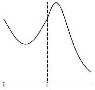
We would like to point out that our approach for studying positive single-lobe states for the NLS-log on tadpole could be used also to study other branches of standing wave profiles such as positive two-lobe states as in Angulo [7] (see Figure 3 below) or for other metric graphs such as looping edge graphs, a graph consisting of a circle with several half-lines attached at a single vertex (see Figure 7 in Section 6).

Refer to caption
Figure 3: A positive two-lobe state profile on a tadpole graph

The paper is organized as follows. In Section 2, we establish a local and global well-posedness results for the NLS-log model on a tadpole graph. In Section 3, we show the linearization of the NLS-log around a positive single-lobe state and its relation with the self-adjoint operators $\mathcal{L}_{1},\mathcal{L}_{2}$. In Section 4, we show Theorems 1.3-1.4 via our splitting eigenvalue lemma (Lemma 4.4). In Section 5, we give proof of the existence of positive single-lobe states and their stability by the flow of the NLS-log model. Lastly, in Appendix we briefly establish some tools and applications of the extension theory of Krein and von Neumann used in our study, as well as, a Perron-Frobenius property for $\delta$-interactions Schrödinger operators on the line. We also establish the orbital stability criterion from Grillakis&Shath&Strauss in [28] adapted to our interests.


Notation. Let $-\infty\leq a<b\leq\infty$. We denote by $L^{2}(a,b)$ the Hilbert space equipped with the inner product $(u,v)=\int\limits_{a}^{b}u(x)\overline{v(x)}dx$. By $H^{n}(\Omega)$ we denote the classical Sobolev spaces on $\Omega\subset\mathbb{R}$ with the usual norm. We denote by $\mathcal{G}$ the tadpole graph parametrized by the set of edges $\mathbb{E}=\{e_{0},e_{1}\}$, where $e_{0}=[-L,L]$ and $e_{1}=[L,+\infty)$, and attached to the common vertex $\nu=L$. On the graph $\mathcal{G}$ we define the spaces

$$L^{p}(\mathcal{G})=L^{p}(-L,L)\oplus L^{p}(L,+\infty),\;\;\,p>1,$$

with the natural norms. Also, for $\textbf{U}=(u_{1},g_{1}),\textbf{V}=(v_{1},h_{1})\in L^{2}(\mathcal{G})$, the inner product on $L^{2}(\mathcal{G})$ is defined by

$$\langle\textbf{U},\textbf{V}\rangle=\int_{-L}^{L}u_{1}(x)\overline{v_{1}(x)}dx+\int_{L}^{\infty}g_{1}(x)\overline{h_{1}(x)}dx.$$

Let $A$ be a closed densely defined symmetric operator in the Hilbert space $H$. The domain of $A$ is denoted by $D(A)$. The deficiency indices of $A$ are denoted by $n_{\pm}(A):=\dim ker(A^{*}\mp iI)$, with $A^{*}$ denoting the adjoint operator of $A$. The number of negative eigenvalues counting multiplicities (or Morse index) of $A$ is denoted by $n(A)$.

2 Global well-posedness in $\widetilde{W}$

In this section we show that the Cauchy problem associated with the NLS-log model on a tadpole graph is global well-posedness in the space $\widetilde{W}$. From Definition (1.2) this information is crucial for a stability theory. We start with the following technical result.

Lemma 2.1.

Let $W(\mathcal{G})$ and $\widetilde{W}$ be the Banach space defined by

$\displaystyle W(\mathcal{G})=\{(f,g)\in\mathcal{E}(\mathcal{G}):|g|^{2}Log|g|^{2}\in L^{1}(L,+\infty)\},$ (2.1)
$\displaystyle\widetilde{W}=\{(f,g)\in\mathcal{E}(\mathcal{G}):xg\in L^{2}(L,\infty)\}.$

Then $\widetilde{W}\subset W(\mathcal{G})$.

Proof.
  • 1)

    Let’s start by proving that $\widetilde{W}\subset L^{1}(\mathcal{G})$. For $(\varphi,\xi)\in\widetilde{W}$ and the Cauchy-Schwarz inequality we have

    $\displaystyle\int_{-L}^{L}|\varphi|dx+\int_{L}^{\infty}|\xi|dx$ $\displaystyle=\int_{-L}^{L}|\varphi|dx+\int_{L}^{\infty}x|\xi|\frac{1}{x}dx$
    $\displaystyle\leq 2L\sup_{[-L,L]}|\varphi|+\left(\int_{L}^{\infty}x^{2}|\xi|^{2}dx\right)^{\frac{1}{2}}\left(\int_{L}^{\infty}\frac{1}{x^{2}}dx\right)^{\frac{1}{2}}<\infty.$
  • 2)

    Let again $(\varphi,\xi)\in\widetilde{W}$, then

    $$\int_{L}^{\infty}|\xi|^{2}|Log|\xi||dx=\int_{\{x\in[L,\infty):|\xi(x)|<1\}}|\xi|^{2}|Log|\xi||dx+\int_{\{x\in[L,\infty):|\xi(x)|\geq 1\}}|\xi|^{2}|Log|\xi||dx.$$ (2.2)

    Note also that

    $$|Log|\xi(x)|<\frac{1}{|\xi(x)|}\ \ \text{for}\ \ |\xi(x)|<1,\ \ \text{and}\ \ |Log|\xi(x)|<|\xi(x)|\ \ \text{for}\ \ |\xi(x)|\geq 1.$$ (2.3)

    Since $\xi\in H^{1}([L,\infty))$, there exist $k>L$ such that $|\xi|<1$ for $[L,\infty)\setminus[L,k]$. Thus, from (2.2), (2.3), and the inclusion $\widetilde{W}\subset L^{1}(\mathcal{G})$ we get

    $\displaystyle\int_{L}^{\infty}|\xi|^{2}|Log|\xi||dx$ $\displaystyle\leq\int_{\{x\in(k,\infty):|\xi|<1\}}|\xi|dx+\int_{\{x\in[L,k]:|\xi|\geq 1\}}|\xi|^{3}dx.$
    $\displaystyle\leq\int_{\{x\in(k,\infty):|\xi|<1\}}|\xi|dx+(k-L)\sup_{[L,k]}|\xi|^{3}<\infty.$

The assertion is proved. ∎

Theorem 2.2.

For any $\mathbf{U_{0}}\in\widetilde{W}$, there is a unique solution $\mathbf{U}\in C(\mathbb{R},\widetilde{W})$ of (1.2) such that $\mathbf{U}(0)=\mathbf{U}_{0}$. Furthermore, the conservation of energy and mass hold, i.e, for any $t\in\mathbb{R}$, we have $E(\mathbf{U}(t))=E(\mathbf{U}_{0})$ and $Q(\mathbf{U}(t))=Q(\mathbf{U}_{0})$.

Proof.

The idea of the proof is to use the approach proposed in [22] (see also [21]) introducing the “reduced” Cauchy problem

$$\left\{\begin{array}[]{ll}i\partial_{t}\mathbb{U}_{n}+\Delta\mathbb{U}_{n}+\mathbb{U}_{n}\mathbb{F}_{n}(|\mathbb{U}_{n}|^{2})=\mathbb{0},\\ \mathbb{U}_{n}(0)=\mathbf{U}_{0}\in\widetilde{W},\end{array}\right.$$ (2.4)

where for $\mathbb{U}_{n}=(u_{n},v_{n})$, $\mathbb{U}_{n}\mathbb{F}_{n}(|\mathbb{U}_{n}|^{2})=(u_{n}f_{n}(|u_{n}|^{2}),v_{n}f_{n}(|v_{n}|^{2})$, $f_{n}(s)=\inf\{n,sup\{-n,f(s)\}\}$, and $f(s)=log(s)$, $s>0$. Next, each $f_{n}$ is Lipschitz continuous from $\mathbb{R}^{+}$ to $\mathbb{R}$ and $\Delta$ with domain $D_{0}$ is a self-adjoint non-positive operator in $L^{2}(\mathcal{G})$ (see Remark 2.3), then the assumptions of Theorem 3.3.1 in [22] hold.

Now, analogous to Lemma 2.3.5 in [22], we can show that there exists solution $\mathbb{U}$ of (1.2) in the sense of distributions (which appears to be weak-$*$ limit of solutions $\mathbb{U}_{n_{k}}$ of Cauchy problem (2.4) which preserve continuity at the vertex $\nu=L$) such that conservation of charge holds. Further, the conservation of energy $E(\mathbb{U})$ defined by (1.13) follows from its monotonicity. Thus, inclusion $\mathbb{U}\in C(\mathbb{R},H^{1}(\mathcal{G}))$ follows from conservation laws. Lastly, for $\mathbf{U}_{0}=(g,h)$, that the condition $xh\in L^{2}(L,+\infty)$ implies that $xv\in L^{2}(L,+\infty)$, it repeats one of Lemma 7.6.2 from [23]. This finishes the proof. ∎

Remark 2.3.

By considering $(-\Delta_{Z},D_{Z})$, $-\Delta_{Z}=-\Delta$, it is possible to see the following (see Angulo&Plaza [13], Noja&Pelinovsky [35]): for every $Z\in\mathbb{R}$ the essential spectrum of the self-adjoint operator $-\Delta_{Z}$ is purely absolutely continuous and $\sigma_{ess}(-\Delta_{Z})=\sigma_{ac}(-\Delta_{Z})=[0,\infty)$. If $Z>0$ then $-\Delta_{Z}$ has exactly one negative eigenvalue, i.e., its point spectrum is $\sigma_{pt}(-\Delta_{Z})=\{-\varrho_{{}_{Z}}^{2}\}$, where $\varrho_{{}_{Z}}>0$ is the only positive root of the trascendental equation

$$\varrho\left(2\tanh\Big{(}\varrho L\Big{)}+1\right)-Z=0,$$

and with eigenfunction

$$\boldsymbol{\Phi}_{Z}=\begin{pmatrix}\cosh(x\varrho_{{}_{Z}}),\;\;x\in[-L,L]\\ \\ e^{-x\varrho_{{}_{Z}}},\;\;\;\;\;\;\;x\in[L,+\infty)\end{pmatrix}.$$

If $Z\leqq 0$ then $-\Delta_{Z}$ has no point spectrum, $\sigma_{pt}(-\Delta_{Z})=\varnothing$. Therefore, for $Z=0$ we have that $-\Delta_{Z}$ is a non-negative operator.

3 Linearization of NLS-log equation

For fixed $c\in\mathbb{R}$, let $U(x,t)=e^{ict}\Theta_{c}(x)$ be a standing wave solution for (1.2) with $\Theta_{c}(x)=(\phi_{c}(x),\psi_{c}(x))\in D_{0}$ being a positive single-lobe state. We consider the the action functional $S_{c}=E+(c+1)Q$, thus $\Theta_{c}$ is a critical point of $S_{c}$. Next, we determine the linear operator associated with the second variational of $S_{c}$ calculated at $\Theta_{c}$, which is crucial for applying the approach in [28]. To express $S^{\prime\prime}_{c}(\Theta_{c})$ it is convenient to split $u,v\in\widetilde{W}$ into real and imaginary parts: $u=u_{1}+iu_{2}$, $v=v_{1}+iv_{2}$. Then, we get $S^{\prime\prime}_{c}(\Theta_{c})(u,v)$ can be formally rewritten as

$\displaystyle S^{\prime\prime}_{c}(\Theta_{c})(u,v)=B_{1}(u_{1},v_{1})+B_{2}(u_{2},v_{2}),$ (3.1)

where

$\displaystyle B_{1}((f,g),(h,q))=$ $\displaystyle\int_{-L}^{L}f^{\prime}h^{\prime}dx+\int_{L}^{\infty}g^{\prime}q^{\prime}dx+\int_{-L}^{L}fh[c-2-Log|\phi_{c}|^{2}]dx$ (3.2)
$\displaystyle+\int_{L}^{\infty}gq[(x-L+a)^{2}-3]dx,$
$\displaystyle B_{2}((f,g),(h,q))=$ $\displaystyle\int_{-L}^{L}f^{\prime}h^{\prime}dx+\int_{L}^{\infty}g^{\prime}q^{\prime}dx+\int_{-L}^{L}fh[c-Log|\psi_{c}|^{2}]dx+\int_{L}^{\infty}gq[(x-L+a)^{2}-1]dx,$

and dom$(B_{i})=\widetilde{W}\times\widetilde{W}$, $i\in\{1,2\}$. Note that the forms $B_{i}$, $i\in\{1,2\}$, are bilinear bounded from below and closed. Therefore, by the First Representation Theorem (see [32], Chapter VI, Section 2.1), they define operators $\widetilde{\mathcal{L}}_{1}$ and $\widetilde{\mathcal{L}}_{2}$ such that for $i\in\{1,2\}$

$\displaystyle\text{dom}(\widetilde{\mathcal{L}}_{i})=\{v\in\widetilde{W}:\exists w\in L^{2}(\mathcal{G})\text{ s.t. }\forall z\in\widetilde{W},B_{i}(v,z)=\langle w,z\rangle\}$ (3.3)
$\displaystyle\widetilde{\mathcal{L}}_{i}v=w.$
Theorem 3.1.

The operators $\widetilde{\mathcal{L}}_{1}$ and $\widetilde{\mathcal{L}}_{2}$ determined in (3.3) are given by

$\displaystyle\widetilde{\mathcal{L}}_{1}=diag\left(-\partial_{x}^{2}+(c-2)-Log|\phi_{c}|^{2},-\partial_{x}^{2}+(x-L+a)^{2}-3\right)$
$\displaystyle\widetilde{\mathcal{L}}_{2}=diag\left(-\partial_{x}^{2}+c-Log|\phi_{c}|^{2},-\partial_{x}^{2}+(x-L+a)^{2}-1\right)$

on the domain $\mathcal{D}=\{(f,g)\in D_{0}:x^{2}g\in L^{2}(L,\infty)\}$. Thus, $\widetilde{\mathcal{L}}_{i}=\mathcal{L}_{i}$ defined in (1.17).

Proof.

Since the proof for $\widetilde{\mathcal{L}}_{2}$ is similar to the one for $\widetilde{\mathcal{L}}_{1}$, we deal with $\widetilde{\mathcal{L}}_{1}$. Let $B_{1}=B^{0}+B^{1}$, where $B^{0}:\mathcal{E}(\mathcal{G})\times\mathcal{E}(\mathcal{G})\rightarrow\mathbb{R}$ and $B^{1}:\widetilde{W}\times\widetilde{W}\rightarrow\mathbb{R}$ are defined by

$$B^{0}\left((f,g),(h,q)\right)=\langle(f^{\prime},g^{\prime}),(h^{\prime},q^{\prime})\rangle,\ \ B^{1}\left((f,g),(h,q)\right)=\langle V_{1}(f,g),(h,q)\rangle,$$ (3.4)

and $V_{1}(f,g)=([c-2-Log|\phi_{c}(x)|^{2}]f,[(x-L+a)^{2}-3]g)$. We denote by $\mathcal{L}^{0}$ (resp. $\mathcal{L}^{1}$) the self-adjoint operator on $L^{2}(\mathcal{G})$ associated (by the First Representation Theorem) with $B^{0}$ (resp. $B^{1}$). Thus,

$\displaystyle\text{dom}(\mathcal{L}^{0})=\{v\in\mathcal{E}(\mathcal{G}):\exists w\in L^{2}(\mathcal{G})\text{ s.t. }\forall z\in\mathcal{E}(\mathcal{G}),B^{0}(v,z)=\langle w,z\rangle\}$
$\displaystyle\mathcal{L}^{0}v=w.$

We claim that $\mathcal{L}^{0}$ is the self-adjoint operator

$$\mathcal{L}^{0}=-\Delta=-\frac{d^{2}}{dx^{2}},\ \ \text{dom}(-\Delta)=D_{0}.$$

Indeed, let $v=(v_{1},v_{2})\in D_{0}$ and $w=-v^{\prime\prime}\in L^{2}(\mathcal{G})$. Then for every $z=(z_{1},z_{2})\in\mathcal{E}(\mathcal{G})$ and using the integration by parts we have

$\displaystyle B^{0}(v,z)$ $\displaystyle=(v^{\prime},z^{\prime})=\int_{-L}^{L}v_{1}^{\prime}z_{1}^{\prime}dx+\int_{L}^{\infty}v_{2}^{\prime}z_{2}^{\prime}dx$
$\displaystyle=v_{1}^{\prime}(L)z_{1}(L)-v_{1}^{\prime}(-L)z_{1}(-L)-v_{2}^{\prime}(L)z_{2}(L)-\int_{-L}^{L}v_{1}^{\prime\prime}z_{1}^{\prime}dx-\int_{L}^{\infty}v_{2}^{\prime\prime}z_{2}^{\prime}dx$
$\displaystyle=(-v^{\prime\prime},z)=(w,z).$

Thus, $v\in$ dom$(\mathcal{L}^{0})$ and $\mathcal{L}^{0}v=w=-v^{\prime\prime}=-\Delta v$. Hence, $-\Delta\subset\mathcal{L}^{0}$. Since $-\Delta$ is self-adjoint on $D_{0}$, $\mathcal{L}^{0}=-\Delta$.

Again, by the First Representation Theorem,

$\displaystyle\text{dom}(\mathcal{L}^{1})=\{v\in\widetilde{W}:\exists w\in L^{2}(\mathcal{G})\text{ s.t. }\forall z\in\widetilde{W},B^{1}(v,z)=\langle w,z\rangle\}$
$\displaystyle\mathcal{L}^{1}v=w.$

Note that $\mathcal{L}^{1}$ is the self-adjoint extension of the following multiplication operator for $u=(f,g)$

$$\mathcal{M}u=V_{1}(f,g),\ \text{dom}(\mathcal{M})=\{u\in\mathcal{E}(\mathcal{G}):V_{1}u\in L^{2}(\mathcal{G})\}.$$

Indeed, for $v\in$ dom$(\mathcal{M})$ we have $v\in\widetilde{W}$, and we define $w=V_{1}v\in L^{2}(\mathcal{G})$. Then for every $z\in\widetilde{W}$ we get $B^{1}(v,z)=\langle w,z\rangle$. Thus, $v\in$ dom$(\mathcal{L}^{1})$ and $\mathcal{L}^{1}v=w=V_{1}v$. Hence, $\mathcal{M}\subset\mathcal{L}^{1}$. Since $\mathcal{M}$ is self-adjoint, $\mathcal{L}^{1}=\mathcal{M}$. The proof of the Theorem is complete. ∎

4 Proof of theorems 1.3 and 1.4

Let us consider one a priori positive single-lobe state $(\phi_{c},\psi_{c})$ solution for (1.8) with $c\in\mathbb{R}$. By convenience we denote $\phi=\phi_{c}$ and $\psi=\psi_{c}$. Thus, the linearized operator $\mathcal{L}_{1}$ in Theorem 3.1 becomes as

$$\mathcal{L}_{1}=diag(-\partial_{x}^{2}+(c-2)-Log|\phi|^{2},-\partial_{x}^{2}+(c-2)-Log|\psi|^{2})$$ (4.1)

with domain $\mathcal{D}=\{(f,g)\in D_{0}:x^{2}g\in L^{2}([L,\infty))\}$.

Next, for $(f,g)\in\mathcal{D}$ we consider $h(x)=g(x+L)$ for $x>0$. Then $h(0)=g(L)$ and $h^{\prime}(0)=g^{\prime}(L)$. Therefore, the eigenvalue problem $\mathcal{L}_{1}(f,g)^{t}=\lambda(f,g)^{t}$ will be equivalent to the following one

$$\left\{\begin{array}[]{ll}\mathcal{L}_{0,1}f(x)=\lambda f(x),\ \ \ x\in(-L,L),\\ \mathcal{L}_{1,1}h(x)=\lambda h(x),\ \ \ x\in(0,+\infty),\\ (f,h)\in D,\end{array}\right.$$ (4.2)

where

$$\mathcal{L}_{0,1}=-\partial_{x}^{2}+(c-2)-Log|\phi|^{2},\ \ \ \mathcal{L}_{1,1}\equiv-\partial_{x}^{2}+(c-2)-Log|\psi_{0,a}|^{2},$$ (4.3)

and $\psi_{0,a}(x)=e^{\frac{c+1}{2}}e^{-\frac{(x+a)^{2}}{2}}$, with $x>0$, $a>0$. The domain $D_{+}$ is given by

$$D_{+}=\{(f,h)\in X^{2}(-L,L):f(L)=f(-L)=h(0),f^{\prime}(L)-f^{\prime}(-L)=h^{\prime}(0),x^{2}h\in L^{2}(0,+\infty)\},$$ (4.4)

with $X^{n}(-L,L)\equiv H^{n}(-L,L)\oplus H^{n}(0,+\infty)$, $n\in\mathbb{N}$. We note that $(\phi,\psi_{0,a})\in D_{+}$.

For the convenience of notation, we will consider $\psi_{a}=\psi_{0,a}$. We define $\mathcal{L_{+}}=diag(\mathcal{L}_{0,1},\mathcal{L}_{1,1})$ with domain $D_{+}$. The proof of the Theorem 1.3 will follow from sections 4.1 and 4.2 below.

4.1 Perron-Frobenius property and Morse index for $(\mathcal{L}_{+},D_{+})$

Initially, we will see that $n(\mathcal{L}_{+})\geqq 1$. In fact, since $(\phi,\psi_{a})\in D_{+}$ and

$$\begin{array}[]{ll}\langle\mathcal{L}_{+}(\phi,\psi_{a})^{t},(\phi,\psi_{a})^{t}\rangle&=-2\left[\int_{-L}^{L}\phi^{2}(x)dx+\int_{0}^{+\infty}\psi_{a}^{2}(x)dx\right]<0,\end{array}$$ (4.5)

we obtain from the mini-max principle that $n(\mathcal{L}_{+})\geqq 1$. Now, we note that is possible to show, via the extension theory for symmetric operators of Krein-von Neumann, that $n(\mathcal{L}_{+})\leqq 2$.

Theorem 4.1.

The Morse index associated to $(\mathcal{L}_{+},D_{+})$ is one. Thus, the Morse index for $(\mathcal{L}_{1},\mathcal{D})$ is also one.

The proof of Theorem 4.1 is based on the following Perron-Frobenius property (PF property) for $(\mathcal{L}_{+},D_{+})$. Our approach is based on EDO’s techniques and draws in the ideas of Angulo in [7, 6]. At the end of this section, we give the proof of Theorem 4.1.

4.1.1 Perron-Frobenius property for $(\mathcal{L}_{+},D_{+})$

We start our analysis by defining the quadratic form $\mathcal{Q}$ associated to operator $\mathcal{L}_{+}$ on $D_{+}$, namely, $\mathcal{Q}:D(\mathcal{Q})\to\mathbb{R}$, with

$$\mathcal{Q}(\eta,\zeta)=\int_{-L}^{L}(\eta^{\prime})^{2}+V_{\phi}\eta^{2}dx+\int_{0}^{+\infty}(\zeta^{\prime})^{2}+W_{\psi}\zeta^{2}dx,$$ (4.6)

$V_{\phi}=(c-2)-Log|\phi|^{2}$, $W_{\psi}=(c-2)-Log|\psi_{a}|^{2}=(x+a)^{2}-3$, and $D(\mathcal{Q})$ defined by

$$D(\mathcal{Q})=\{(\eta,\zeta)\in X^{1}(-L,L):\eta(L)=\eta(-L)=\zeta(0),x\zeta\in L^{2}(0,+\infty)\}.$$ (4.7)
Theorem 4.2.

Let $\lambda_{0}<0$ be the smallest eigenvalue for $\mathcal{L}_{+}$ on $D_{+}$ with associated eigenfunction $(\eta_{\lambda_{0}},\zeta_{\lambda_{0}})$. Then, $\eta_{\lambda_{0}},\zeta_{\lambda_{0}}$ are positive functions. Moreover, $\eta_{\lambda_{0}}$ is even on $[-L,L]$.

Proof.

We split the proof into several steps.

  1. 1)

    The profile $\zeta_{\lambda_{0}}$ is not identically zero: Indeed, suppose $\zeta_{\lambda_{0}}\equiv 0$, then $\eta_{\lambda_{0}}$ satisfies

    $$\left\{\begin{array}[]{ll}\mathcal{L}_{0,1}\eta_{\lambda_{0}}(x)=\lambda_{0}\eta_{\lambda_{0}}(x),\quad\quad x\in(-L,L),\\ \eta_{\lambda_{0}}(L)=\eta_{\lambda_{0}}(-L)=0\\ \eta^{\prime}_{\lambda_{0}}(L)=\eta^{\prime}_{\lambda_{0}}(-L).\end{array}\right.$$ (4.8)

    From the Dirichlet condition and oscillations theorems of the Floquet theory we need to have that $\eta_{\lambda_{0}}$ is odd. Then, by Sturm-Liouville theory there is an eigenvalue $\theta$ for $\mathcal{L}_{0,1}$, such that $\theta<\lambda_{0}$, with associated eigenfunction $\xi>0$ on $(-L,L)$, and $\xi(-L)=\xi(L)=0$.

    Now, let $\mathcal{Q}_{Dir}$ be the quadratic form associated to $\mathcal{L}_{0,1}$ with Dirichlet domain, namely, $\mathcal{Q}_{Dir}:H^{1}_{0}(-L,L)\to\mathbb{R}$ and

    $$\mathcal{Q}_{Dir}(f)=\int_{-L}^{L}(f^{\prime})^{2}+V_{\phi}f^{2}dx.$$ (4.9)

    Then, $\mathcal{Q}_{Dir}(\xi)=\mathcal{Q}(\xi,0)\geqq\lambda_{0}\|\xi\|^{2}$ and so, $\theta\geqq\lambda_{0}$. It which is a contradiction.

  2. 2)

    $\zeta_{\lambda_{0}}(0)\neq 0$: suppose $\zeta_{\lambda_{0}}(0)=0$ and we consider the odd-extension $\zeta_{odd}$ for $\zeta_{\lambda_{0}}$, and the even-extension $\psi_{even}$ of the tail-profile $\psi_{a}$ on all the line. Then, $\zeta_{odd}\in H^{2}(\mathbb{R})$ and $\psi_{even}\in H^{2}(\mathbb{R}-\{0\})\cap H^{1}(\mathbb{R})$. Next, we consider the following unfold operator $\widetilde{\mathcal{L}}$ associated to $\mathcal{L}_{1,1}$,

    $$\widetilde{\mathcal{L}}=-\partial_{x}^{2}+(c-2)-Log|\psi_{even}|^{2},$$ (4.10)

    on the $\delta$-interaction domain

    $$D_{\delta,\gamma}=\{f\in H^{2}(\mathbb{R}-\{0\})\cap H^{1}(\mathbb{R}):x^{2}f\in L^{2}(\mathbb{R}),f^{\prime}(0+)-f^{\prime}(0-)=\gamma f(0)\}$$ (4.11)

    for any $\gamma\in\mathbb{R}$. Then, from the extension theory for symmetric operators (see Remark 4.2 item (iii) in [10]) and Proposition 8.3 in Appendix) we have that the family $(\widetilde{\mathcal{L}},D_{\delta,\gamma})_{\gamma\in\mathbb{R}}$ represents all the self-adjoint extensions of the symmetric operator $(\mathcal{M}_{0},D(\mathcal{M}_{0}))$ defined by

    $$\mathcal{M}_{0}=\widetilde{\mathcal{L}},\quad D(\mathcal{M}_{0})=\{f\in H^{2}(\mathbb{R}):x^{2}f\in L^{2}(\mathbb{R}),f(0)=0\},$$

    with deficiency indices given by $n_{\pm}(\mathcal{M}_{0})=1$ (see Theorem 4.11 in [10]). Now, the even tail-profile $\psi_{even}$ satisfies $\psi_{even}^{\prime}(x)\neq 0$ for all $x\neq 0$, and so from the well-defined relation

    $$\mathcal{M}_{0}f=-\frac{1}{\psi^{\prime}_{even}}\frac{d}{dx}\Big{[}(\psi^{\prime}_{even})^{2}\frac{d}{dx}\Big{(}\frac{f}{\psi^{\prime}_{even}}\Big{)}\Big{]},\quad x\neq 0$$ (4.12)

    we can see easily that $\langle\mathcal{M}_{0}f,f\rangle\geqq 0$ for all $f\in D(\mathcal{M}_{0})$. Therefore, from the extension theory (see Proposition 8.4 in Appendix) we obtain that the Morse index for the family $(\widetilde{\mathcal{L}},D_{\delta,\gamma})$ satisfies $n(\widetilde{\mathcal{L}})\leqq 1$, for all $\gamma\in\mathbb{R}$. So, since $\zeta_{odd}\in D_{\delta,\gamma}$ (for any $\gamma$) and $\widetilde{\mathcal{L}}\zeta_{odd}=\lambda_{0}\zeta_{odd}$ on $\mathbb{R}$, we have $n(\widetilde{\mathcal{L}})=1$. Then, $\lambda_{0}$ will be the smallest negative eigenvalue for $\widetilde{\mathcal{L}}$ on $\delta$-interactions domains in (4.11) and by Theorem 8.6 in Appendix (Perron Frobenius property for $\widetilde{\mathcal{L}}$ with $\delta$-interactions domains on the line), $\zeta_{odd}$ needs to be positive which is a contradiction. Therefore, $\zeta_{\lambda_{0}}(0)\neq 0$.

  3. 3)

    $\zeta_{\lambda_{0}}:[0,+\infty)\to\mathbb{R}$ can be chosen strictly positive: Without loss of generality we suppose $\zeta_{\lambda_{0}}(0)>0$. Then the condition $\eta^{\prime}_{\lambda_{0}}(L)-\eta^{\prime}_{\lambda_{0}}(-L)=\zeta^{\prime}_{\lambda_{0}}(0)$ implies

    $$\zeta^{\prime}_{\lambda_{0}}(0)=\Big{[}\frac{\eta^{\prime}_{\lambda_{0}}(L)-\eta^{\prime}_{\lambda_{0}}(-L)}{\zeta_{\lambda_{0}}(0)}\Big{]}\zeta_{\lambda_{0}}(0)\equiv\gamma_{0}\zeta_{\lambda_{0}}(0).$$

    Next, we consider $\zeta_{even}$ being the even-extension of $\zeta_{\lambda_{0}}$ to all the line, then $\zeta_{even}\in D_{\delta,2\gamma_{0}}$ and $\widetilde{\mathcal{L}}\zeta_{even}=\lambda_{0}\zeta_{even}$. Thus, a similar analysis as in item 2) above implies that $\lambda_{0}$ is the smallest eigenvalue for $(\widetilde{\mathcal{L}},D_{\delta,2\gamma_{0}})$. Hence $\zeta_{even}$ is strictly positive on $\mathbb{R}$. Therefore, $\zeta_{\lambda_{0}}(x)>0$ for all $x\geqq 0$.

  4. 4)

    $\eta_{\lambda_{0}}:[-L,L]\to\mathbb{R}$ can be chosen strictly positive: initially we have that $\eta_{\lambda_{0}}$ satisfies the following boundary condition,

    $$\eta^{\prime}_{\lambda_{0}}(L)-\eta^{\prime}_{\lambda_{0}}(-L)=\Big{[}\frac{\zeta^{\prime}_{\lambda_{0}}(0)}{\zeta_{\lambda_{0}}(0)}\Big{]}\zeta_{\lambda_{0}}(0)\equiv\alpha_{0}\zeta_{\lambda_{0}}(0)=\alpha_{0}\eta_{\lambda_{0}}(L).$$

    Now, we consider the following eigenvalue problem for $\mathcal{L}_{0,1}$ in (4.3) with real coupled self-adjoint boundary condition determined by $\alpha\in\mathbb{R}$,

    $$(RC_{\alpha}):\;\;\left\{\begin{array}[]{ll}\mathcal{L}_{0,1}y(x)=\beta y(x),\quad\quad x\in(-L,L),\\ y(L)=y(-L),\\ y^{\prime}(L)-y^{\prime}(-L)=\alpha y(L).\end{array}\right.$$ (4.13)

    Next, from Theorem 1.35 in Kong&Wu&Zettl [33] or Theorem 4.8.1 in Zettl [38] with $K=[k_{ij}]$ given by $k_{11}=1$, $k_{12}=0$, $k_{21}=\alpha_{0}$ and $k_{22}=1$, we obtain that the first eigenvalue $\beta_{0}=\beta_{0}(K)$ for (4.13) with $\alpha=\alpha_{0}$ is simple. Moreover, since the pair $(\eta_{\lambda_{0}},\lambda_{0})$ is a solution for (4.13), we have $\lambda_{0}\geqq\beta_{0}$. In the following we show $\lambda_{0}=\beta_{0}$. Indeed, we consider the quadratic form associated to the $(RC_{\alpha_{0}})$-problem in (4.13), $\mathcal{Q}_{RC}$, where for $h\in H^{1}(-L,L)$ with $h(L)=h(-L)$,

    $$\mathcal{Q}_{RC}(h)=\int_{-L}^{L}(h^{\prime})^{2}+V_{\phi}h^{2}dx-\alpha_{0}|h(L)|^{2}.$$ (4.14)

    Next, define $\xi=\nu\zeta_{\lambda_{0}}$ with $\nu$ being a real constant to be chosen such that $\xi(0)=\nu\zeta_{\lambda_{0}}(0)=h(L)$. Thus, $(h,\xi)\in D(\mathcal{Q})$ in (4.7). Now, by using that $\mathcal{L}_{1,1}\zeta_{\lambda_{0}}=\lambda_{0}\zeta_{\lambda_{0}}$ we obtain,

    $\displaystyle\mathcal{Q}_{RC}(h)$ $\displaystyle=\mathcal{Q}(h,\xi)-\alpha_{0}h^{2}(L)-\int_{0}^{+\infty}(\xi^{\prime})^{2}+W_{\psi}\xi^{2}dx$ (4.15)
    $\displaystyle=\mathcal{Q}(h,\xi)-\alpha_{0}h^{2}(L)+\nu^{2}\zeta^{\prime}_{\lambda_{0}}(0)\zeta_{\lambda_{0}}(0)-\lambda_{0}\nu^{2}\|\zeta_{\lambda_{0}}\|^{2}$
    $\displaystyle=\mathcal{Q}(h,\xi)-\xi^{\prime}_{\lambda_{0}}(0)h(L)+h(L)\xi^{\prime}_{\lambda_{0}}(0)-\lambda_{0}\|\xi\|^{2}$
    $\displaystyle=\mathcal{Q}(h,\xi)-\lambda_{0}\|\xi\|^{2}\geqq\lambda_{0}[\|h\|^{2}+\|\xi\|^{2}]-\lambda_{0}\|\xi\|^{2}=\lambda_{0}\|h\|^{2}.$

    Then, $\beta_{0}\geqq\lambda_{0}$ and so $\beta_{0}=\lambda_{0}$.

    By the analysis above, we get that $\lambda_{0}$ is the first eigenvalue for the problem $(RC_{\alpha_{0}})$ in (4.13) and so it is simple. Then, $\eta_{\lambda_{0}}$ is odd or even. If $\eta_{\lambda_{0}}$ is odd, then the condition $\eta_{\lambda_{0}}(L)=\eta_{\lambda_{0}}(-L)$ implies $\eta_{\lambda_{0}}(L)=0$. But, $\eta_{\lambda_{0}}(L)=\zeta_{\lambda_{0}}(0)>0$. So, we need to have that $\eta_{\lambda_{0}}$ is even. Now, from Oscillation Theorem $(RC_{\alpha_{0}})$-problem, the number of zeros of $\eta_{\lambda_{0}}$ on $[-L,L)$ is 0 or 1 (see Theorem 4.8.5 in [38]). Since $\eta_{\lambda_{0}}(-L)>0$ and $\eta_{\lambda_{0}}$ is even, we obtain necessarily that $\eta_{\lambda_{0}}>0$ on $[-L,L]$. This finishes the proof.

Corollary 4.3.

Let $\lambda_{0}<0$ be the smallest eigenvalue for $(\mathcal{L}_{+},D_{+})$. Then, $\lambda_{0}$ is simple.

Proof.

The proof is immediate. Suppose $\lambda_{0}$ is double. Then, there is $(f_{0},g_{0})^{t}$-eigenfunction associated to $\lambda_{0}$ orthogonal to $(\eta_{\lambda_{0}},\zeta_{\lambda_{0}})$. By Theorem 4.2 we have that $f_{0},g_{0}>0$. So, we arrive at a contradiction from the orthogonality property of the eigenfunctions. ∎

4.1.2 Splitting eigenvalue method on tadpole graphs

In the following, we establish our main strategy for studying eigenvalue problems on a tadpole graph $\mathcal{G}$ deduced in Angulo [7]. More exactly, we reduce the eigenvalue problem for $\mathcal{L}_{1}\equiv diag(\mathcal{L}_{1}^{0},\mathcal{L}_{1}^{1})$ in (1.17) to two classes of eigenvalue problems, one for $\mathcal{L}_{1}^{0}=-\partial_{x}^{2}+(c-2)-Log|\phi|^{2}$ with periodic boundary conditions on $[-L,L]$ and the other for the operator $\mathcal{L}_{1}^{1}=-\partial_{x}^{2}+(c-2)-Log|\psi|^{2}$ with Neumann type boundary conditions on $[L,+\infty)$.

Lemma 4.4.

It consider $(\mathcal{L}_{1},\mathcal{D})$ in Theorem 1.3. Suppose $(f,g)\in\mathcal{D}$ with $g(L)\neq 0$ and $\mathcal{L}_{1}(f,g)^{t}=\gamma(f,g)^{t}$, for $\gamma\leq 0$. Then, we obtain the following two eigenvalue problems:

$$\left\{\begin{array}[]{ll}\mathcal{L}_{1}^{0}f(x)=\gamma f(x),\;x\in(-L,L),\\ f(L)=(-L),\;\;f^{\prime}(L)=f^{\prime}(-L),\end{array}\right.\;\qquad\left\{\begin{array}[]{ll}\mathcal{L}_{1}^{1}=\gamma g(x),\;x>L,\\ g^{\prime}(L+)=0.\end{array}\right.$$
Proof.

For $(f,g)\in\mathcal{D}$ and $g(L)\neq 0$, we have

$$f(-L)=f(L),\;\;f^{\prime}(L)-f^{\prime}(-L)=\left[\frac{g^{\prime}(L+)}{g(L)}\right]f(L)\equiv\theta f(L),$$

and so $f$ satisfies the real coupled problem $(RC_{\alpha})$ in (4.13) with $\alpha=\theta$ and $\beta=\gamma$. Then, from the proof of Lemma 3.4 in [7] we obtain that $\theta=0$ and so we prove the Lemma. ∎

Remark 4.5.

From Lemma 4.4 follows that $\eta_{\lambda_{0}}$ in Theorem 4.2 remains a even-periodic function on $[-L,L]$ and $\zeta_{\lambda_{0}}$ satisfies Neumann boundary condition on $[L,+\infty)$.

4.1.3 Morse index for $(\mathcal{L}_{+},D_{+})$

In the following, we give the proof of Theorem 4.1.

Proof.

We consider $\mathcal{L}_{+}$ on $D_{+}$ and suppose $n(\mathcal{L}_{+})=2$ without loss of generality (we note that via extension theory we can show $n(\mathcal{L}_{+})\leqq 2$). From Theorem 4.2 and Corollary 4.3, the first negative eigenvalue $\lambda_{{0}}$ for $\mathcal{L}_{+}$ is simple with an associated eigenfunction $(\eta_{{\lambda_{0}}},\zeta_{{\lambda_{0}}})$ having positive components and $\eta_{\lambda_{0}}$ being even on $[-L,L]$. Therefore, for $\lambda_{{1}}$ being the second negative eigenvalue for $\mathcal{L}_{+}$, we need to have $\lambda_{1}>\lambda_{0}$.

Let $(f_{{1}},g_{{}_{1}})\in D_{+}$ be an associated eigenfunction to $\lambda_{{1}}$. In the following, we divide our analysis into several steps.

  1. 1)

    Suppose $g_{{1}}\equiv 0$: then $f_{{1}}(-L)=f_{{1}}(L)=0$ and $f_{{1}}$ odd (see step 1) in the proof of Theorem 4.2). Now, our profile-solution $\phi$ satisfies

    $$\mathcal{L}_{0,1}\phi^{\prime}=0,\;\phi^{\prime}\;\text{is odd},\,\phi^{\prime}(x)>0,\;\text{for}\;x\in[-L,0),$$

    thus since $\lambda_{1}<0$ we obtain from the Sturm Comparison Theorem that there is $r\in(-L,0)$ such that $\phi^{\prime}(r)=0$, which is a contradiction. Then, $g_{1}$ is non-trivial.

  2. 2)

    Suppose $g_{1}(0+)=0$: we consider the odd-extension $g_{1,odd}\in H^{2}(\mathbb{R})$ of $g_{1}$ and the unfold operator $\widetilde{\mathcal{L}}$ in (4.10) on the $\delta$-interaction domains $D_{\delta,\gamma}$ in (4.11). Then, $g_{1,odd}\in D_{\delta,\gamma}$ for any $\gamma$ and so by Perron-Frobenius property for $(\widetilde{\mathcal{L}},D_{\delta,\gamma})$ (see Appendix) we need to have that $n(\widetilde{\mathcal{L}})\geqq 2$. But, by step $2)$ in the proof of Theorem 4.2 we obtain $n(\widetilde{\mathcal{L}})\leqq 1$ for all $\gamma$, and so we get a contradiction.

  3. 3)

    Suppose $g_{1}(0+)>0$ (without loss of generality): we will see that $g_{{1}}(x)>0$ for all $x>0$. Indeed, by Lemma 4.4 we get $g^{\prime}_{{1}}(0+)=0$. Thus, by considering the even-extension $g_{1,even}$ of $g_{{1}}$ on all the line and the unfold operator $\widetilde{\mathcal{L}}$ in (4.10) on $D_{\delta,0}$, we have that $g_{1,even}\in D_{\delta,0}$ and so $n(\widetilde{\mathcal{L}})\geqq 1$. But, we known that $n(\widetilde{\mathcal{L}})\leqq 1$ and so $\lambda_{{1}}$ is the smallest eigenvalue for $(\widetilde{\mathcal{L}},D_{\delta,0})$. Therefore, by the Perron-Frobenius property for $(\widetilde{\mathcal{L}},D_{\delta,0})$ (see Appendix) $g_{{1}}$ is strictly positive. We note that as $D_{\delta,0}=\{f\in H^{2}(\mathbb{R}):x^{2}f\in L^{2}(\mathbb{R})\}$ follows from classical oscillation theory (see Theorem 3.5 in [16]) that $g_{1,even}>0$.

  4. 4 )

    Lastly, since the pairs $(\zeta_{{\lambda_{0}}},\lambda_{{0}})$ and $(g_{1},\lambda_{1})$ satisfy the eigenvalue problem

    $$\left\{\begin{array}[]{ll}\mathcal{L}_{1,1}g(x)=\gamma g(x),\;x>0,\\ g^{\prime}(0+)=0,\end{array}\right.$$ (4.16)

    follows the property that $\zeta_{{\lambda_{0}}}$ and $g_{1}$ need to be orthogonal (which is a contradiction). This finishes the proof.

4.2 Kernel for $(\mathcal{L}_{1},\mathcal{D})$

In the following, we study the nullity index for $\mathcal{L}_{1}$ on $\mathcal{D}$ (see item $4)$ in Theorem 1.3. Using the notation at the beginning of this section is sufficient to show the following.

Theorem 4.6.

It consider $\mathcal{L}_{+}=diag(\mathcal{L}_{0,1},\mathcal{L}_{1,1})$ on $D_{+}$. Then, the kernel associated with $\mathcal{L}_{+}$ on $D_{+}$ is trivial.

Proof.

Let $(f,h)\in D_{+}$ such that $\mathcal{L}_{+}(f,h)^{t}={\bf{0}}$. Thus, since $\mathcal{L}_{1,1}h=0$ and $\mathcal{L}_{1,1}\psi^{\prime}_{a}=0$, we obtain from classical Sturm-Liouville theory on half-lines ([16]) that there is $b\in\mathbb{R}$ with $h=b\psi^{\prime}_{a}$ on $(0,+\infty)$. Next, we have the following cases:

  1. 1)

    Suppose $b=0$: then $h\equiv 0$ and $f$ satisfies $\mathcal{L}_{0,1}f=0$ with Dirichlet-periodic conditions

    $$f(L)=f(-L)=0,\;\;\text{and}\;\;f^{\prime}(L)=f^{\prime}(-L).$$

    Suppose $f\neq 0$. From oscillation theory of the Floquet theory, Sturm-Liouville theory for Dirichlet conditions, $\mathcal{L}_{0,1}\phi^{\prime}=0$ on $[-L,L]$, $\phi^{\prime}$ odd and $\phi^{\prime}(L)\neq 0$, we get $f\equiv 0$ and so $ker(\mathcal{L}_{+})$ is trivial (see proof of Theorem 1.4 in [7]).

  2. 2)

    Suppose $b\neq 0$: then $h(0)\neq 0$ ($h(x)>0$ without loss of generality with $b<0$). Hence, from the splitting eigenvalue result in Lemma 4.4, we obtain that $f$ satisfies

    $$\left\{\begin{array}[]{ll}\mathcal{L}_{0,1}f(x)=0,\;x\in[-L,L],\\ f(L)=f(-L)=h(0)>0,\;\;\text{and}\;\;f^{\prime}(L)=f^{\prime}(-L),\end{array}\right.$$ (4.17)

    and $h^{\prime}(0)=0$. The last equality implies immediately $\psi^{\prime\prime}_{a}(0)=0$, therefore if we have for $\alpha=\psi^{\prime\prime}_{a}(0)$ that $\alpha\neq 0$, we obtain a contradiction. Then, $b=0$ and by item $1)$ above $ker(\mathcal{L}_{+})=\{{\bf{0}}\}$.

    Next, we consider the case $\alpha=0$. Then, initially, by Floquet theory and oscillation theory, we have the following partial distribution of eigenvalues, $\beta_{n}$ and $\mu_{n}$, associated to $\mathcal{L}_{0,1}$ with periodic and Dirichlet conditions, respectively,

    $$\beta_{0}<\mu_{0}<\beta_{1}\leqq\mu_{1}\leqq\beta_{2}<\mu_{2}<\beta_{3}.$$ (4.18)

    In the following, we will see $\beta_{1}=0$ in (4.18) and it is simple. Indeed, by (4.18) suppose that $0>\mu_{1}$. Now, we know that $\mathcal{L}_{0,1}\phi^{\prime}=0$ on $[-L,L]$, $\phi^{\prime}$ is odd and $\phi^{\prime}(x)>0$ for $[-L,0)$, and the eigenfunction associated with $\mu_{1}$ is odd, therefore from Sturm Comparison Theorem we get that $\phi^{\prime}$ need to have one zero on $(-L,0)$, which is impossible. Hence, $0\leqq\mu_{1}$. Next, suppose that $\mu_{1}=0$ and let $\chi_{1}$ be an odd eigenfunction for $\mu_{1}$. Let $\{\phi^{\prime},P\}$ be a base of solutions for the problem $\mathcal{L}_{0,1}g=0$ (we recall that $P$ can be chosen being even and satisfying $P(0)=1$ and $P^{\prime}(0)=0$). Then, $\chi_{1}=a\phi^{\prime}$ with $0=\chi_{1}(L)=a\phi^{\prime}(L)$. Hence, $\chi_{1}\equiv 0$ which is not possible. Therefore, $0<\mu_{1}$ and so $\beta_{1}=0$ is simple with eigenfunction $f$ (being even or odd). We note that $\beta_{2}$ is also simple.

    Lastly, since $f(-L)=f(L)>0$ follows that $f$ is even and by Floquet theory $f$ has exactly two different zeros $-a,a$ ($a>0$) on $(-L,L)$. Hence, $f(0)<0$. Next, we consider the Wronskian function (constant) of $f$ and $\phi^{\prime}$,

    $$W(x)=f(x)\phi^{\prime\prime}(x)-f^{\prime}(x)\phi^{\prime}(x)\equiv C,\quad\text{for all}\;\;x\in[-L,L].$$

    Then, $C=f(0)\phi^{\prime\prime}(0)>0$. Therefore, by hypotheses ($\alpha=0$ ) we obtain

    $$C=f(L)\phi^{\prime\prime}(L)=h(0)\psi^{\prime\prime}_{a}(0)=0,$$ (4.19)

    which is a contradiction. Then, $b=0$ and by item $1)$ above we get again $ker(\mathcal{L}_{+})=\{{\bf{0}}\}$. This finishes the proof.

4.3 Morse and nullity indices for operator $\mathcal{L}_{2}$

Proof.

$[$Theorem 1.4$]$ We consider a positive single-lobe state $(\phi_{c},\psi_{c})$. Then, from (1.8) we get $(\phi_{c},\psi_{c})\in ker(\mathcal{L}_{2})$. Next, we consider

$$\mathcal{M}=-\partial_{x}^{2}+c-log(\phi_{c}^{2}),\;\;\mathcal{N}=-\partial_{x}^{2}+c-log(\psi_{c}^{2})$$

then for any ${\bf{V}}=(f,g)\in D_{0}$, we obtain

$\displaystyle\mathcal{M}f$ $\displaystyle=-\frac{1}{\phi_{c}}\frac{d}{dx}\Big{[}\phi_{c}^{2}\frac{d}{dx}\Big{(}\frac{f}{\phi_{c}}\Big{)}\Big{]},\quad\;\;x\in(-L,L)$ (4.20)
$\displaystyle\mathcal{N}g$ $\displaystyle=-\frac{1}{\psi_{c}}\frac{d}{dx}\Big{[}\psi_{c}^{2}\frac{d}{dx}\Big{(}\frac{g}{\psi_{c}}\Big{)}\Big{]},\quad\;\;x>L.$

Thus, we obtain immediately

$$\langle\mathcal{L}_{2}{\bf{V}},{\bf{V}}\rangle=\int_{-L}^{L}\phi_{c}^{2}\Big{(}\frac{d}{dx}\Big{(}\frac{f}{\phi_{c}}\Big{)}\Big{)}^{2}dx+\int_{L}^{\infty}\psi_{c}^{2}\Big{(}\frac{d}{dx}\Big{(}\frac{g}{\psi_{c}}\Big{)}\Big{)}^{2}dx\geqq 0.$$

Moreover, since $\langle\mathcal{L}_{2}{\bf{V}},{\bf{V}}\rangle=0$ if and only if $f=d_{1}\phi_{c}$ and $g=d_{2}\psi_{c}$, we obtain from the continuity property at $x=L$ that $d_{1}=d_{2}$. Then, $ker(\mathcal{L}_{2})=span\{(\phi_{c},\psi_{c})\}$. This finishes the proof. ∎

5 Existence of the positive single-lobe state

In this section, our focus is proving the following existence theorem:

Theorem 5.1.

For any $c\in\mathbb{R}$, there is only one single lobe positive state $\Theta_{c}=(\phi_{c},\psi_{c})\in D_{0}$ that satisfies the NLS-log equation (1.7), is monotonically decreasing on $[0,L]$ and $[L,+\infty)$, and the map $c\in\mathbb{R}\mapsto\Theta_{c}\in D_{0}$ is $C^{1}$. Moreover, the mass $\mu(c)=Q(\Theta_{c})$ satisfies $\frac{d}{dc}\mu(c)>0$.

For proving Theorem 5.1 we need some tools from dynamical systems theory for orbits on the plane and so for the convenience of the reader, we will divide our analysis into several steps (sub-sections) in the following.

5.1 The period function

We consider $L=\pi$ (without loss of generality) and $\Psi(x)=\psi(x+\pi)$, $x>0$. Then, the transformation

$$\phi_{0}(x)=e^{\frac{1-c}{2}}\Psi(x),\ \ \phi_{1}(x)=e^{\frac{1-c}{2}}\phi(x)$$ (5.1)

implies that system (1.8)with $Z=0$ is transformed in the following system of differential equations independent of the velocity $c$:

$$\left\{\begin{array}[]{ll}-\phi_{1}^{\prime\prime}(x)+\phi_{1}(x)-log(\phi_{1}^{2}(x))\phi_{1}(x)=0,\;\;\;\;x\in(-\pi,\pi),\\ -\phi_{0}^{\prime\prime}(x)+\phi_{0}(x)-log(\phi_{0}^{2}(x))\phi_{0}(x)=0,\;\;\;\;x>0,\\ \phi_{1}(\pi)=\phi_{1}(-\pi)=\phi_{0}(0),\\ \phi_{1}^{\prime}(\pi)-\phi_{1}^{\prime}(-\pi)=\phi_{0}^{\prime}(0).\end{array}\right.$$ (5.2)

We know that a positive decaying solution to equation $-\phi_{0}^{\prime\prime}+\phi_{0}-log(\phi_{0}^{2})\phi_{0}=0$ on the positive half-line is expressed by

$$\phi_{0}(x)=ee^{\frac{-(x+a)^{2}}{2}},\;\;\;\;x>0,\;\;a\in\mathbb{R}$$ (5.3)

with $\phi_{0}(0)=ee^{\frac{-a^{2}}{2}}$. If $a>0$, $\phi_{0}$ is monotonically decreasing in $[0,\infty)$ (a Gausson tail-profile) and if $a<0$, $\phi_{0}$ is non-monotone on $[0,\infty)$ (a Gausson bump-profile). To prove Theorem 5.1, we will only consider Gausson-tail profiles for $\phi_{0}$, therefore, we need to choose $a>0$.

The second-order differential equations in system (5.2) are integrable with a first-order invariant given by

$$E(\phi,\xi)=\xi^{2}-A(\phi),\ \ \ \xi:=\frac{d\phi}{dx},\ \ \ A(\phi)=2\phi^{2}-log(\phi^{2})\phi^{2}.$$ (5.4)

Note that the value of $E(\phi,\xi)=E$ is independent of $x$. Next, for $A(u)=2u^{2}-log(u^{2})u^{2}$ we have that there is only one positive root of $A^{\prime}(u)=2u(1-log(u^{2}))$ denoted by $r_{*}$ such that $A^{\prime}(r_{*})=0$, in fact, $r_{*}=e^{\frac{1}{2}}$. For $E=0$ there are two homoclinic orbits, one corresponds to positive $u=\phi$ and the other to negative $u=-\phi$. Periodic orbits exist inside each of the two homoclinic loops and correspond to $E\in(E_{*},0)$ where $E_{*}=-A(r_{*})=-e$, and they correspond to either strictly positive $u$ or strictly negative $u$. Periodic orbits outside the two homoclinic loops exist for $E\in(0,\infty)$ and they correspond to sign-indefinite $u$. Note that

$$E+A(r_{*})>0,\ \ \ E\in(E_{*},\infty).$$ (5.5)

The homoclinic orbit with the profile solution (5.3) and $a>0$ corresponds to $\xi=-\sqrt{A(\phi)}$ for all $x>0$. Let us define $r_{0}:=ee^{\frac{-a^{2}}{2}}$, that is, the value of $\phi_{0}(x)$ at $x=0$. Then, $-\sqrt{A(r_{0})}$ is the value of $\phi^{\prime}_{0}$ at $x=0$. Note that :

  • $r_{0}\in\left(0,e\right)$ is a free parameter obtained from $a\in(0,\infty)$.

  • $r_{0}(a)\longrightarrow e$ when $a\longrightarrow 0$.

  • $r_{0}(a)\longrightarrow 0$ when $a\longrightarrow\infty$.

Hence, the profile $\phi_{1}$ will be found from the following boundary-value problem:

$$\left\{\begin{array}[]{ll}-\phi_{1}^{\prime\prime}(x)+\phi_{1}(x)-log(\phi_{1}^{2}(x))\phi_{1}(x)=0,\;\;\;\;x\in(-\pi,\pi),\\ \phi_{1}(\pi)=\phi_{1}(-\pi)=r_{0},\\ \phi_{1}^{\prime}(-\pi)=-\phi_{1}^{\prime}(\pi)=\frac{\sqrt{A(r_{0})}}{2}\end{array}\right.$$ (5.6)

where $r_{0}\in\left(0,e\right)$ will be seen as a free parameter of the problem. The positive single-lobe state $\phi_{1}$ will correspond to a part of the level curve $E(\phi,\xi)=E$ which intersects $r_{0}$ only twice at the ends of the interval $[-\pi,\pi]$ (see Figure 4 for a geometric construction of a positive single-lobe state for (5.6)).

Refer to caption
Figure 4: $\cdot$ Red line: $s_{0}(r_{0})=\frac{1}{2}\sqrt{A(r_{0})}=\frac{1}{2}\phi_{0}^{\prime}(0)$.
\cdot 
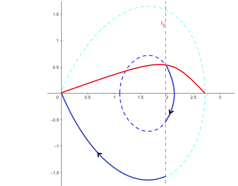
Dashed-dotted vertical line depicts the value of r0=ϕ0(0)=eea2/2r_{0}=\phi_{0}(0)=ee^{-a^{2}/2}.
$\cdot$ The blue dashed curve represents the homoclinic orbit at $E=0$, solid part depicting the shifted-tail NLS-log soliton.
$\cdot$ The level curve $E(\phi,\zeta)=E(r_{0},s_{0})$, at $r_{0}=ee^{-a^{2}/2}$ and $s_{0}=\frac{1}{2}\sqrt{A(p_{0})}$, is shown by the blue dashed line.
$\cdot$ The blue solid parts depict a suitable positive single-lobe state profile solution for the NLS-log.

Let us denote by $s_{0}=\frac{\sqrt{A(r_{0})}}{2}$ and we define the period function for a given $(r_{0},s_{0})$:

$$T_{+}(r_{0},s_{0}):=\int_{r_{0}}^{r_{+}}\frac{d\phi}{\sqrt{E+A(\phi)}},$$ (5.7)

where the value $E$ and the turning point $r_{+}$ are defined from $(r_{0},s_{0})$ by

$$E=s_{0}^{2}-A(r_{0})=-A(r_{+}).$$ (5.8)

For each level curve of $E(\phi,\xi)=E$ inside the homoclinic loop we have $E\in(E_{*},0)$ and the turning point satisfies:

$$0<r_{*}<r_{+}<e.$$ (5.9)

We recall that $\phi_{1}$ is a positive single-lobe solution of the boundary-value problem (5.6) if and only if $r_{0}\in(0,e)$ is a root of the nonlinear equation

$$T(r_{0})=\pi,\ \ \ where\ \ T(r_{0})=T_{+}\left(r_{0},\frac{\sqrt{A(r_{0})}}{2}\right).$$ (5.10)

We note that as $T(r_{0})$ is uniquely defined by $r_{0}\in\left(0,e\right)$, the nonlinear equation (5.10) defines a unique mapping $\left(0,e\right)\ni r_{0}\mapsto T(r_{0})\in(0,\infty)$. In the following sub-section, we show the monotonicity of this function.

5.2 Monotonicity of the period function

In this sub-section, we will use the theory of dynamical systems for orbits on the plane and the period function in (5.7) to prove that the mapping $\left(0,e\right)\ni r_{0}\mapsto T(r_{0})\in(0,\infty)$ is $C^{1}$ and monotonically decreasing.

Recall that if $W(\phi,\xi)$ is a $C^{1}$ function in an open region of $\mathbb{R}^{2}$, then the differential of $W$ is defined by

$$dW(\phi,\xi)=\frac{\partial W}{\partial\phi}d\phi+\frac{\partial W}{\partial\xi}d\xi$$

and the line integral of $dW(\phi,\xi)$ along any $C^{1}$ contour $\gamma$ connecting $(\phi_{0},\xi_{0})$ and $(\phi_{1},\xi_{1})$ does not depend on $\gamma$ and is evaluated as

$$\int_{\gamma}dW(\phi,\xi)=W(\phi_{1},\xi_{1})-W(\phi_{0},\xi_{0}).$$

At the level curve of $E(\phi,\xi)=\xi^{2}-A(\phi)=E$, we can write

$$d\left[\frac{2(A(\phi)-A(r_{*}))\xi}{A^{\prime}(\phi)}\right]=\left[2-\frac{2(A(\phi)-A(r_{*}))A^{\prime\prime}(\phi)}{\left[A^{\prime}(\phi)\right]^{2}}\right]\xi d\phi+\frac{2(A(\phi)-A(r_{*}))}{A^{\prime}(\phi)}d\xi$$ (5.11)

where the quotients are not singular for every $\phi>0$. In view of the fact that $2\xi d\xi=A^{\prime}(\phi)d\phi$ on the level curve $E(\phi,\xi)=E$, we can express (5.11) as:

$$\frac{(A(\phi)-A(r_{*}))}{\xi}d\phi=-\left[2-\frac{2(A(\phi)-A(r_{*}))A^{\prime\prime}(\phi)}{\left[A^{\prime}(\phi)\right]^{2}}\right]\xi d\phi+d\left[\frac{2(A(\phi)-A(r_{*}))\xi}{A^{\prime}(\phi)}\right].$$ (5.12)

The following lemma justifies monotonicity of the mapping $\left(0,e\right)\ni r_{0}\mapsto T(r_{0})\in(0,\infty)$.

Lemma 5.2.

The function $r_{0}\mapsto T(r_{0})$ is $C^{1}$ and monotonically decreasing for every $r_{0}\in\left(0,e\right)$.

Proof.

Since $s_{0}=\frac{\sqrt{A(r_{0})}}{2}$ in (5.10) for a given $r_{0}\in\left(0,e\right)$ we have that the value of $T(r_{0})$ is obtained from the level curve $E(\phi,\xi)=E_{0}(r_{0})$, where

$$E_{0}(r_{0})\equiv s_{0}^{2}-A(r_{0})=-\left(1-\frac{1}{4}\right)A(r_{0})=-\frac{3}{4}A(r_{0}).$$ (5.13)

For every $r_{0}\in\left(0,e\right)$, we use the formula (5.12) to get

$\displaystyle\left[E_{0}(r_{0})+A(r_{*})\right]T(r_{0})$ $\displaystyle=\int_{r_{0}}^{r_{+}}\left[\xi-\frac{A(\phi)-A(r_{*})}{\xi}\right]d\phi$ (5.14)
$\displaystyle=\int_{r_{0}}^{r_{+}}\left[3-\frac{2(A(\phi)-A(r_{*}))A^{\prime\prime}(\phi)}{\left[A^{\prime}(\phi)\right]^{2}}\right]\xi d\phi+\frac{2(A(r_{0})-A(r_{*}))s_{0}}{A^{\prime}(r_{0})},$

where, we use (5.8) to obtain that $\xi=0$ at $\phi=r_{+}$ and $\xi=s_{0}$ at $\phi=r_{0}$. Because the integrands are free of singularities and $E_{0}(r_{0})+A(r_{*})>0$ due to (5.5), the mapping $\left(0,e\right)\ni r_{0}\mapsto T(r_{0})\in(0,\infty)$ is $C^{1}$. We only need to prove that $T^{\prime}(r_{0})<0$ for every $r_{0}\in\left(0,e\right)$.

Differentiating (5.14) with respect to $r_{0}$ yields

$\displaystyle\left[E_{0}(r_{0})+A(r_{*})\right]T^{\prime}(r_{0})=$ $\displaystyle\left([E_{0}(r_{0})+A(r_{*})]T(r_{0})\right)^{\prime}-E_{0}^{\prime}(r_{0})T(p_{0})$ (5.15)
$\displaystyle=$ $\displaystyle\int_{r_{0}}^{r_{+}}\left[3-\frac{2(A(\phi)-A(r_{*}))A^{\prime\prime}(\phi)}{\left[A^{\prime}(\phi)\right]^{2}}\right]\frac{\partial\xi}{\partial r_{0}}d\phi-\left[3-\frac{2(A(r_{0})-A(r_{*}))A^{\prime\prime}(r_{0})}{\left[A^{\prime}(r_{0})\right]^{2}}\right]s_{0}$
$\displaystyle+\left[2-\frac{2(A(r_{0})-A(r_{*}))A^{\prime\prime}(r_{0})}{\left[A^{\prime}(r_{0})\right]^{2}}\right]s_{0}+\frac{2(A(r_{0})-A(r_{*}))}{A^{\prime}(r_{0})}s_{0}^{\prime}-E_{0}^{\prime}(r_{0})\int_{r_{0}}^{r_{+}}\frac{d\phi}{\xi}$
$\displaystyle=$ $\displaystyle-\frac{A(r_{*})}{4s_{0}}-\frac{3A^{\prime}(r_{0})}{8}\int_{r_{0}}^{r_{+}}\left[1-\frac{2(A(\phi)-A(r_{*}))A^{\prime\prime}(\phi)}{\left[A^{\prime}(\phi)\right]^{2}}\right]\frac{d\phi}{\xi},$

where we have used

$$s_{0}=\frac{2A(r_{0})s_{0}^{\prime}}{A^{\prime}(r_{0})},\ \ \ E_{0}^{\prime}(r_{0})=-\frac{3A^{\prime}(r_{0})}{4},\ \ \ s_{0}^{\prime}(r_{0})=\frac{A^{\prime}(r_{0})}{8s_{0}},\ \ \ \frac{\partial\xi}{\partial s_{0}}=\frac{E_{0}^{\prime}(r_{0})}{2\xi}.$$

As $A(\phi)=2\phi^{2}-log(\phi^{2})\phi^{2}$, we obtain that (5.15) is as follows:

$$[E_{0}(r_{0})+A(r_{*})]T^{\prime}(r_{0})=-\frac{A(r_{*})}{4s_{0}}-\frac{3A^{\prime}(r_{0})}{8}\int_{r_{0}}^{r_{+}}\frac{\phi^{2}(3-log(\phi^{2}))-e(1+log(\phi^{2}))}{\phi^{2}(1-log(\phi^{2}))^{2}\xi}d\phi.$$ (5.16)

Let us define the following function:

$$f(\phi)=\phi^{2}(3-log(\phi^{2}))-e(1+log(\phi^{2})).$$ (5.17)
Refer to caption
Figure 5: Graph of $f$ in (5.17)

Differentiating (5.17) with respect to $\phi$ yields:

$\displaystyle f^{\prime}(\phi)=2\phi(2-log(\phi^{2}))-\frac{2e}{\phi}$ (5.18)
$\displaystyle\Leftrightarrow$ $\displaystyle\;\;\phi f^{\prime}(\phi)=2\phi^{2}(2-log(\phi^{2}))-2e\ \ \ \ \ \ \ (\phi>0).$

Note that $f^{\prime}(\phi)=0\Leftrightarrow\phi=r_{*}$ and $f^{\prime}(\phi)<0$ for any $\phi\in(0,r_{*})\cup(r_{*},+\infty)$. Since $f(\phi)=0\Leftrightarrow\phi=r_{*}$ we have that $f(\phi)>0$ for any $\phi\in(0,r_{*})$ and $f(\phi)<0$ for any $\phi\in(r_{*},+\infty)$.

Next, we know that $A^{\prime}(r_{0})<0$ for any $r_{0}\in(r_{*},e)$ and $f(\phi)<0$ for $\phi\in[r_{0},r_{+}]\subset(r_{*},e)$ then follows that $T^{\prime}(r_{0})<0$. Similarly, since $A^{\prime}(r_{*})=0$, we have $T^{\prime}(r_{*})<0$.

Now, we consider the case $r_{0}\in(0,r_{*})$. Then,

$\displaystyle\int_{r_{0}}^{r_{+}}\frac{\phi^{2}(3-log(\phi^{2}))-e(1+log(\phi^{2}))}{\phi^{2}(1-log(\phi^{2}))^{2}\xi}d\phi=I_{1}+I_{2}$ (5.19)

where

$\displaystyle I_{1}$ $\displaystyle=\int_{r_{0}}^{r_{*}}\frac{\phi^{2}(3-log(\phi^{2}))-e(1+log(\phi^{2}))}{\phi^{2}(1-log(\phi^{2}))^{2}\xi}d\phi,$ (5.20)
$\displaystyle I_{2}$ $\displaystyle=\int_{r_{*}}^{r_{+}}\frac{\phi^{2}(3-log(\phi^{2}))-e(1+log(\phi^{2}))}{\phi^{2}(1-log(\phi^{2}))^{2}\xi}d\phi$

Because $f(\phi)>0$ for any $\phi\in(0,r_{*})$, $I_{1}>0$. By using $A^{\prime}(\phi)=2\phi(1-log(\phi^{2}))$ we get that (see Figure 6)

$$\frac{\phi^{2}(3-log(\phi^{2}))-e(1+log(\phi^{2}))}{\phi^{2}(1-log(\phi^{2}))^{2}}>\frac{A^{\prime}(\phi)}{2\phi^{3}}\ \ \text{for any }\phi\in(r_{*},e)\supset(r_{*},r_{+}).$$ (5.21)
Refer to caption
Figure 6: Inequality in (5.21)

By (5.21) and proceeding by integration by parts we have

$\displaystyle I_{2}$ $\displaystyle>\int_{r_{*}}^{r_{+}}\frac{A^{\prime}(\phi)}{2\phi^{3}\sqrt{E_{0}(r_{0})+A(\phi)}}d\phi$ (5.22)
$\displaystyle=-\frac{\sqrt{E_{0}(r_{0})+A(r_{*})}}{r_{*}^{3}}+3\int_{r_{*}}^{r_{+}}\frac{\sqrt{E_{0}(r_{0})+A(\phi)}}{\phi^{4}}d\phi$
$\displaystyle=-\frac{\sqrt{E_{0}(r_{0})+A(r_{*})}}{r_{*}^{3}}+3\int_{r_{*}}^{r_{+}}\frac{\xi}{\phi^{4}}d\phi$

Substituting this into (5.16) yields

$\displaystyle\left[E_{0}(r_{0})+A(r_{*})\right]T^{\prime}(r_{0})$ $\displaystyle=-\frac{A(r_{*})}{4s_{0}}-\frac{3A^{\prime}(r_{0})}{8}I_{1}-\frac{3A^{\prime}(r_{0})}{8}I_{2}$ (5.23)
$\displaystyle<-\frac{A(r_{*})}{4s_{0}}+\frac{3A^{\prime}(r_{0})}{8}\frac{\sqrt{E_{0}(r_{0})+A(r_{*})}}{r_{*}^{3}}-\frac{3A^{\prime}(r_{0})}{8}I_{1}$
$\displaystyle\ \ \ -\frac{9A^{\prime}(r_{0})}{8}\int_{r_{*}}^{r_{+}}\frac{\xi}{\phi^{4}}d\phi.$

To evaluate the first two terms we will use that $A(r_{*})=e$, $s_{0}=\frac{\sqrt{A(r_{0})}}{2}$, and $\max_{r_{0}\in(0,r_{*})}A^{\prime}(r_{0})=4e^{-\frac{1}{2}}$, so that we get

$\displaystyle-\frac{A(r_{*})}{4s_{0}}+\frac{3A^{\prime}(r_{0})}{8}\frac{\sqrt{E_{0}(r_{0})+A(r_{*})}}{r_{*}^{3}}$ $\displaystyle=-\frac{e}{2\sqrt{A(r_{0})}}+\frac{3A^{\prime}(r_{0})}{8}\frac{\sqrt{E_{0}(r_{0})+e^{c}}}{e^{\frac{3}{2}}}$ (5.24)
$\displaystyle<-\frac{e}{2\sqrt{A(r_{0})}}+\frac{3\sqrt{E_{0}(r_{0})+e}}{2e^{2}}.$

For (5.13) we get

$\displaystyle-\frac{e}{2\sqrt{A(r_{0})}}$ $\displaystyle+\frac{3\sqrt{E_{0}(r_{0})+e}}{2e^{2}}<0\Leftrightarrow\frac{3\sqrt{E_{0}(r_{0})+e}}{2e^{2}}<\frac{e}{2\sqrt{A(r_{0})}}\Leftrightarrow\frac{9(E_{0}(r_{0})+e)}{4e^{4}}<\frac{e^{2}}{4A(r_{0})}$ (5.25)
$\displaystyle\Leftrightarrow-\frac{27A(r_{0})}{4}+9e<\frac{e^{6}}{A(r_{0})}\Leftrightarrow 9e<\frac{e^{6}}{A(r_{0})}+\frac{27A(r_{0})}{4}.$

Since $A^{\prime}(r_{0})>0$ for any $r_{0}\in(0,r_{*})$, $A(r_{0})$ increases monotonically for any $r_{0}\in(0,r_{*})$, and $\frac{1}{A(r_{0})}$ decreases monotonically for any $r_{0}\in(0,r_{*})$. Differentiating $\frac{e^{6}}{A(r_{0})}+\frac{27A(r_{0})}{4}$ with respect to $r_{0}$ yields

$\displaystyle\left(\frac{e^{6}}{A(r_{0})}+\frac{27A(r_{0})}{4}\right)^{\prime}$ $\displaystyle=-\frac{e^{6}A^{\prime}(r_{0})}{(A(r_{0}))^{2}}+\frac{27A^{\prime}(r_{0})}{4}<-\frac{e^{6}A^{\prime}(r_{0})}{(A(r_{*}))^{2}}+\frac{27A^{\prime}(r_{0})}{4}$ (5.26)
$\displaystyle=-e^{4}A^{\prime}(r_{0})+\frac{27A^{\prime}(r_{0})}{4}=\left(\frac{27}{4}-e^{4}\right)A^{\prime}(r_{0})<0.$

Therefore, the function $\frac{e^{6}}{A(r_{0})}+\frac{27A(r_{0})}{4}$ is monotonically decreasing for any $r_{0}\in(0,r_{*})$. Using this we get that

$$\frac{e^{6}}{A(r_{0})}+\frac{27A(r_{0})}{4}>\frac{e^{6}}{A(r_{*})}+\frac{27A(r_{*})}{4}=\left(e^{4}+\frac{27}{4}\right)e>9e$$ (5.27)

Thus, for (5.25) we get

$$-\frac{A(r_{*})}{4s_{0}}+\frac{3A^{\prime}(r_{0})}{8}\frac{\sqrt{E_{0}(r_{0})+A(r_{*})}}{r_{*}^{3}}<0\ \ \text{for any }r_{0}\in(0,r_{*}).$$

As a result of the above calculations, for every $r_{0}\in(0,r_{*})$ we have $T^{\prime}(r_{0})<0$. This finishes the proof.

5.3 Proof of Theorem 5.1

Proof.

Due to the monotony of the period function $T(r_{0})$ in $r_{0}$ given by Lemma 5.2 we have a diffeomorphism $\left(0,e\right)\ni r_{0}\mapsto T(r_{0})\in(0,\infty)$. In fact, we will show that $T(r_{0})\longrightarrow 0$ when $r_{0}\longrightarrow e$ and $T(r_{0})\longrightarrow\infty$, when $r_{0}\longrightarrow 0$. Indeed, from (5.8), (5.13) and (5.9), we have that for $r_{0}\in(0,e)$, the equation $E_{0}(r_{0})=-A(r_{+})$ determines $r_{+}=r_{+}(r_{0})$ from the nonlinear equation:

$$2r_{+}^{2}-log(r_{+}^{2})r_{+}^{2}=\frac{3}{4}[2r_{0}^{2}-log(r_{0}^{2})r_{0}^{2}],$$ (5.28)

and $\lim_{r_{0}\rightarrow e}\frac{3}{4}[2r_{0}^{2}-log(r_{0}^{2})r_{0}^{2}]=0$. Now for (5.28) we have

$\displaystyle 2r_{+}^{2}-log(r_{+}^{2})r_{+}^{2}\rightarrow 0,\text{ when}\ r_{0}\rightarrow e$ $\displaystyle\Leftrightarrow r_{+}\rightarrow e,\text{ when}\ r_{0}\rightarrow e$ (5.29)
$\displaystyle\Leftrightarrow|r_{+}-r_{0}|\rightarrow 0,\text{ when}\ r_{0}\rightarrow e.$

Since the weakly singular integrand below is integrable, we have

$$T(r_{0})=\int_{r_{0}}^{r_{+}}\frac{d\phi}{\sqrt{E+A(\phi)}}=\int_{r_{0}}^{r_{+}}\frac{d\phi}{\sqrt{A(\phi)-A(r_{+})}}\rightarrow 0,\text{ when}\ r_{0}\rightarrow e,$$ (5.30)

Next, for every $0<r_{0}<r_{+}<e$ we obtain

$\displaystyle T(r_{0})=\int_{r_{0}}^{r_{+}}$ $\displaystyle\frac{d\phi}{\sqrt{A(\phi)-A(p_{+})}}\geq\int_{r_{0}}^{r_{+}}\frac{d\phi}{\sqrt{A(\phi)}}$ (5.31)
$\displaystyle=\int_{r_{0}}^{r_{+}}\frac{d\phi}{\sqrt{2\phi^{2}-log(\phi^{2})\phi^{2}}}=\int_{r_{0}}^{r_{+}}\frac{d\phi}{\phi\sqrt{2-log(\phi^{2})}}.$

Since $r_{+}\in(r_{*},e)$ and

$$\lim_{r_{0}\rightarrow 0}\frac{3}{4}[2r_{0}^{2}-log(r_{0}^{2})r_{0}^{2}]=0,$$

by (5.28) we have $r_{+}\rightarrow e,\text{ when}\ r_{0}\rightarrow 0$. Therefore, as

$$\int_{0}^{e}\frac{d\phi}{\phi\sqrt{(2-log(\phi^{2})}}=\lim_{\phi\rightarrow 0}\sqrt{2-log(\phi^{2})}=+\infty$$

we have $T(r_{0})\rightarrow+\infty$ as $r_{0}\rightarrow 0$. Then, as the function $T(r_{0})$ is monotone decreasing, the codomain of the function $r_{0}\mapsto T(r_{0})$ is indeed $(0,+\infty)$.

Thus, there is a unique $r_{0}\in(0,e)$ such that $T(r_{0})=\pi$. Therefore, the boundary-value problem (5.6) has a solution. Next, define $a_{0}>0$ such that $ee^{\frac{-a_{0}^{2}}{2}}=r_{0}$. Then,

$$\phi_{c}(x)=e^{\frac{c-1}{2}}\phi_{1}(x)\;\;\text{and}\;\;\psi_{c}(x)=e^{\frac{c+1}{2}}e^{\frac{-(x-\pi+a_{0})^{2}}{2}}$$

satisfies (1.8) with $Z=0$. Obviously, we have that $\mathbb{R}\ni c\mapsto\Theta(c)=(\phi_{c},\psi_{c})\in D_{0}$ is a $C^{1}$-mapping of positive single-lobe state for the NLS-log equation on the tadpole graph.

Next, the relation

$$\mu(c)=\|\Theta(c)\|^{2}=e^{c-1}\Big{[}\int_{-\pi}^{\pi}\phi_{1}^{2}(x)dx+\int_{0}^{+\infty}\phi_{0}^{2}(x)dx\Big{]}$$

with $\phi_{0}(x)=ee^{\frac{-(x+a_{0})^{2}}{2}}$ and $\phi_{1}$ independent of $c$, implies $\mu^{\prime}(c)>0$ for all $c\in\mathbb{R}$. The proof of the theorem is completed.

6 Proof of the stability theorem

In this section, we show Theorem 1.5 based on the stability criterion in Theorem 8.7 (Appendix).

Proof.

By Theorem 5.1 we obtain the existence of a $C^{1}$-mapping $c\in\mathbb{R}\rightarrow\Theta_{c}=(\phi_{c},\psi_{c})$ of positive single-lobe states for the NLS-log model on a tadpole graph. Moreover, the mapping $c\to\|\Theta_{c}\|^{2}$ is strictly increasing. Next, from Theorem 1.3 we get that the Morse index for $\mathcal{L}_{1}$ in (1.17), $n(\mathcal{L}_{1})$, satisfies $n(\mathcal{L}_{1})=1$ and $ker(\mathcal{L}_{1})=\{\bf{0}\}$. Moreover, Theorem 1.4 establishes that $Ker(\mathcal{L}_{2})=span\{(\phi_{c},\psi_{c})\}$ and $\mathcal{L}_{2}\geqq 0$. Thus, by Theorem 2.2 and stability criterion in Theorem 8.7, we obtain that $e^{ict}(\phi_{c},\psi_{c})$ is orbitally stable in $\widetilde{W}$. This finishes the proof. ∎

7 Discussion and open problems

In this paper, we have established the existence and orbital stability of standing wave solutions for the NLS-log model on a tadpole graph with a profile being a positive single-lobe state. To that end, we use tools from dynamical systems theory for orbits on the plane and we use the period function for showing the existence of a positive single-lobe state with Neumann-Kirchhoff condition at the vertex $\nu=L$ ($Z=0$ in (1.8)). The orbital stability of these profiles is based on the framework of Grillakis et al. in [28] adapted to the tadpole graph and so via a splitting eigenvalue method and tools of the extension theory of Krein&von Neumann for symmetric operators and Sturm Comparison Theorem we identify the Morse index and the nullity index of a specific linearized operator around of an a priori positive single-lobe state which is fundamental ingredients in this endeavor. For the case $Z\neq 0$ in (1.8) and by supposing a priori the existence of a positive single-lobe state is possible to obtain similar results for $(\mathcal{L}_{2},D_{Z})$ as in Theorem 1.4. Statements $1)-2)-3)$ in Theorem (1.3) are also true for $(\mathcal{L}_{1},D_{Z})$ (see Section 3 in [6]). Moreover, if we define the quantity for the shift $a=a(Z)$

$$\alpha(a)=\frac{\psi^{\prime\prime}_{c}(L)}{\psi^{\prime}_{c}(L)}+Z=\frac{1-a^{2}}{a}+Z,$$

then, the kernel associated with $(\mathcal{L}_{1},D_{Z})$ is trivial in the following cases: for $\alpha\neq 0$ or $\alpha=0$ in the case of admissible parameters $Z$ satisfying $Z\leqq 0$ (see Theorem 1.3 and Lemma 3.5 in [6]). The existence of these profiles with $Z\neq 0$ will be addressed in future work. Our approach has a prospect of being extended to study stability properties of other standing wave states for the NLS-log on a tadpole graph (by instance, to choose boundary conditions in the family of 6-parameters given in (1.5)) or on another non-compact metric graph such as a looping edge graph (see Figure 7 below), namely, a graph consisting of a circle with several half-lines attached at a single vertex (see [7, 6, 12]).

$-L$ $+L$

Figure 7: A looping edge graph with $N=5$ half-lines

8 Appendix

8.1 Classical extension theory results

The following results are classical in the extension theory of symmetric operators and can be found in [34, 37]. Let $A$ be a closed densely defined symmetric operator in the Hilbert space $H$. The domain of $A$ is denoted by $D(A)$. The deficiency indices of $A$ are denoted by $n_{\pm}(A):=\dim Ker(A^{*}\mp iI)$, with $A^{*}$ denoting the adjoint operator of $A$. The number of negative eigenvalues counting multiplicities (or Morse index) of $A$ is denoted by $n(A)$.

Theorem 8.1 (von-Neumann decomposition).

Let $A$ be a closed, symmetric operator, then

$$D(A^{*})=D(A)\oplus\mathcal{N}_{-i}\oplus\mathcal{N}_{+i}.$$ (8.1)

with $\mathcal{N}_{\pm i}=\ker(A^{*}\mp iI)$. Therefore, for $u\in D(A^{*})$ and $u=x+y+z\in D(A)\oplus\mathcal{N}_{-i}\oplus\mathcal{N}_{+i}$,

$$A^{*}u=Ax+(-i)y+iz.$$ (8.2)
Remark 8.2.

The direct sum in (8.1) is not necessarily orthogonal.

Proposition 8.3.

Let $A$ be a densely defined, closed, symmetric operator in some Hilbert space $H$ with deficiency indices equal $n_{\pm}(A)=1$. All self-adjoint extensions $A_{\theta}$ of $A$ may be parametrized by a real parameter $\theta\in[0,2\pi)$ where

$$\begin{split}D(A_{\theta})&=\{x+c\phi_{+}+\zeta e^{i\theta}\phi_{-}:x\in D(A),\zeta\in\mathbb{C}\},\\ A_{\theta}(x+\zeta\phi_{+}+\zeta e^{i\theta}\phi_{-})&=Ax+i\zeta\phi_{+}-i\zeta e^{i\theta}\phi_{-},\end{split}$$

with $A^{*}\phi_{\pm}=\pm i\phi_{\pm}$, and $\|\phi_{+}\|=\|\phi_{-}\|$.

The following proposition provides a strategy for estimating the Morse-index of the self-adjoint extensions (see [34], [37]-Chapter X).

Proposition 8.4.

Let $A$ be a densely defined lower semi-bounded symmetric operator (that is, $A\geq mI$) with finite deficiency indices, $n_{\pm}(A)=k<\infty$, in the Hilbert space ${H}$, and let $\widehat{A}$ be a self-adjoint extension of $A$. Then the spectrum of $\widehat{A}$ in $(-\infty,m)$ is discrete and consists of, at most, $k$ eigenvalues counting multiplicities.

The next Proposition can be found in Naimark [34] (see Theorem 9).

Proposition 8.5.

All self-adjoint extensions of a closed, symmetric operator which has equal and finite deficiency indices have one and the same continuous spectrum.

8.2 Perron-Frobenius property for $\delta$-interaction Schrödinger operators on the line

In this section, we establish the Perron-Frobenius property for the unfold self-adjoint operator $\widetilde{\mathcal{L}}$ in (4.10),

$$\widetilde{\mathcal{L}}=-\partial_{x}^{2}+(c-2)-Log(\psi_{even}^{2})=-\partial_{x}^{2}+(|x|+a)^{2}-3$$ (8.3)

on $\delta$-interaction domains, namely,

$$D_{\delta,\gamma}=\{f\in H^{2}(\mathbb{R}-\{0\})\cap H^{1}(\mathbb{R}):x^{2}f\in L^{2}(\mathbb{R}),f^{\prime}(0+)-f^{\prime}(0-)=\gamma f(0)\}$$ (8.4)

for any $\gamma\in\mathbb{R}$. Here, $\psi_{even}$ is the even extension to whole the line of the Gausson tail-soliton profile $\psi_{a}(x)=e^{\frac{c+1}{2}}e^{-\frac{(x+a)^{2}}{2}}$, with $x>0$, $a>0$. Since

$$\lim\limits_{|x|\to+\infty}(|x|+a)^{2}=+\infty,$$

operator $\widetilde{\mathcal{L}}$ has a discrete spectrum, $\sigma(\widetilde{\mathcal{L}})=\sigma_{d}(\widetilde{\mathcal{L}})=\{\lambda_{k}\}_{k\in\mathbb{N}}$ (this statement can be obtained similarly using the strategy in the proof of Theorem 3.1 in [16]). In particular, from subsections 2-3 in Chapter 2 in [16] adapted to $(\widetilde{\mathcal{L}},D_{\delta,\gamma})$ for $\gamma$ fixed (see also Lemma 4.8 in [10]) we have the following distribution of the eigenvalues $\lambda_{0}<\lambda_{1}<\cdot\cdot\cdot<\lambda_{k}<\cdot\cdot\cdot$, with $\lambda_{k}\to+\infty$ as $k\to+\infty$ and from the semi-boundedness of $V_{a}=(|x|+a)^{2}-3$ we obtain that any solution of the equation $\widetilde{\mathcal{L}}v=\lambda_{k}v$, $v\in D_{\delta,\gamma}$, is unique up to a constant factor. Therefore each eigenvalue $\lambda_{k}$ is simple.

Theorem 8.6.

$[$ Perron-Frobenius property $]$ Consider the family of self-adjoint operators $(\widetilde{\mathcal{L}},D_{\delta,\gamma})_{\gamma\in\mathbb{R}}$. For $\gamma$ fixed, let $\lambda_{0}=\inf\sigma_{p}(\widetilde{\mathcal{L}})$ be the smallest eigenvalue. Then, the corresponding eigenfunction $\zeta_{0}$ to $\lambda_{0}$ is positive (after replacing $\zeta_{0}$ by $-\zeta_{0}$ if necessary) and even.

Proof.

This result can be obtained by following the strategy in the proof of Theorem 3.5 in [16]. Here, we give another approach via a slight twist of standard abstract Perron-Frobenius arguments (see Proposition 2 in Albert&Bona&Henry [4]). The basic point in the analysis is to show that the Laplacian operator $-\Delta_{\gamma}\equiv-\frac{d^{2}}{dx^{2}}$ on the domain $D_{\delta,\gamma}$ has its resolvent $R_{\mu}=(-\Delta_{\gamma}+\mu)^{-1}$ represented by a positive kernel for some $\mu>0$ sufficiently large. Namely, for $f\in L^{2}(\mathbb{R})$

$$R_{\mu}f(x)=\int_{-\infty}^{+\infty}K(x,y)f(y)dy$$

with $K(x,y)>0$ for all $x,y\in\mathbb{R}$. By the convenience of the reader we show this main point, the remainder of the proof follows the same strategy as in [4]. Thus, for $\gamma$ fixed, let $\mu>0$ be sufficiently large (with $-2\sqrt{\mu}<\gamma$ in the case $\gamma<0$), then from the Krein formula (see Theorem 3.1.2 in [5]) we obtain

$$K(x,y)=\frac{1}{2\sqrt{\mu}}\Big{[}e^{-\sqrt{\mu}|x-y|}-\frac{\gamma}{\gamma+2\sqrt{\mu}}e^{-\sqrt{\mu}(|x|+|y|)}\Big{]}.$$

Moreover, for every $x$ fixed, $K(x,\cdot)\in L^{2}(\mathbb{R})$. Thus, the existence of the integral above is guaranteed by Holder’s inequality. Moreover, $x^{2}R_{\mu}f\in L^{2}(\mathbb{R})$. Now, since $K(x,y)=K(y,x)$, it is sufficient to show that $K(x,y)>0$ in the following cases.

  1. (1)

    Let $x>0$ and $y>0$ or $x<0$ and $y<0$: for $\gamma\geqq 0$, we obtain from $\frac{\gamma}{\gamma+2\sqrt{\mu}}<1$ and $|x-y|\leqq|x|+|y|$, that $K(x,y)>0$. For $\gamma<0$ and $-2\sqrt{\mu}<\gamma$, it follows immediately $K(x,y)>0$.

  2. (2)

    Let $x>0$ and $y<0$: in this case,

    $$K(x,y)=\frac{1}{\gamma+2\sqrt{\mu}}e^{-\sqrt{\mu}(x-y)}>0$$

    for any value of $\gamma$ (where again $-2\sqrt{\mu}<\gamma$ in the case $\gamma<0$) .

This finishes the proof. ∎

8.3 Orbital stability criterion

For the convenience of the reader, in this subsection we adapted the abstract stability results from Grillakis&Shatah&Strauss in [28] for the case of the NLS-log on tadpole graph. This criterion was used in the proof of Theorem 1.5 for the case of standing waves being positive single-lobe states.

Theorem 8.7.

Suppose that there is $C^{1}$-mapping $c\to(\phi_{c},\psi_{c})$ of standing-wave solutions for the NLS-log model (1.2) on a tadpole graph. We consider the operators $\mathcal{L}_{1}$ and $\mathcal{L}_{2}$ in (1.17). For $\mathcal{L}_{1}$ suppose that the Morse index is one and its kernel is trivial. For $\mathcal{L}_{2}$ suppose that it is a non-negative operator with kernel generated by the profile $(\phi_{c},\psi_{c})$. Moreover, suppose that the Cauchy problem associated with the NLS-log model (1.2) is global well-posedness in the space $\widetilde{W}$ in (1.12). Then, $e^{ict}(\phi_{c},\psi_{c})$ is orbitally stable in $\widetilde{W}$ if $\frac{d}{dc}||(\phi_{c},\psi_{c})||^{2}>0$.

Data availability No data was used for the research described in the article.

Acknowledgements. J. Angulo was partially funded by CNPq/Brazil Grant and him would like to thank to Mathematics Department of the Federal University of Pernambuco (UFPE) by the support and the warm stay during the Summer-program/2025, where part of the present project was developed. A. Pérez was partially funded by CAPES/Brazil and UNIVESP/São Paulo/Brazil.

References

  • [1] R. Adami, E. Serra, and P. Tilli, NLS ground states on graphs, Calc. Var., 54 (2015), no. 1, 743–761.
  • [2] R. Adami, E. Serra, and P. Tilli, Threshold phenomena and existence results for NLS ground states on graphs, J. Funct. Anal., 271 (2016), 201–223.
  • [3] R. Adami, E. Serra, and P. Tilli, Negative energy ground states for the $L^{2}$-critical NLSE on metric graphs, Comm. Math. Phys. 352 (2017), 387–406.
  • [4] J. P. Albert, J.L. Bona, and D. Henry, Sufficient conditions for stability of solitary-wave solutions of model equations for long waves, Physica D: Nonlinear Phenomena, 24 (1987), 343–366.
  • [5] S. Albeverio, F. Gesztesy, R. Hoegh-Krohn, and H. Holden, Solvable models in quantum mechanics, 2nd edition, AMS Chelsea Publishing, Providence, RI, 2005.
  • [6] J. Angulo, Stability theory for the NLS equation on looping edge graphs, Mathematische Zeitschrift, 308 (2024), no. 1, Paper No. 19.
  • [7] J. Angulo, Stability theory for two-lobe states on the tadpole graph for the NLS equation, Nonlinearity 37 (2024), no. 4, Paper No 045015, 43 pp.
  • [8] J. Angulo and A.H. Ardila, Stability of standing waves for logarithmic Schrödinger equation with attractive delta potential, IUMJ, 67 (2018), 471–494.
  • [9] J. Angulo and M. Cavalcante, Nonlinear Dispersive Equations on Star Graphs, $32^{o}$ Colóquio Brasileiro de Matemática, IMPA, (2019).
  • [10] J. Angulo and N. Goloshchapova, Stability of standing waves for NLS-log equation with $\delta$-interaction, Nonlinear Differential Equations Appl. (NoDEA), 24 (2017), Art. 27, 23 pp.
  • [11] J. Angulo and N. Goloshchapova, Extension theory approach in the stability of the standing waves for the NLS equation with point interactions on a star graph, Adv. Differential Equations, 23 (11-12), (2018), 793–846.
  • [12] J. Angulo and A. Munoz, Airy and Schrödinger-type equations on looping edge graphs, ArXiv:2410.11729v2/2024.
  • [13] J. Angulo and R. Plaza, Dynamics of the sine-Gordon on tadpole graphs. Pre-print/2024.
  • [14] A. H. Ardila, Logarithmic NLS equation on star graphs: Existence and stability of standing waves, Differential and Integral Equations, 30 (2017), 735–762.
  • [15] A. H. Ardila, Stability of ground states for logarithmic Schrödinger equation with a $delta^{{}^{\prime}}$-interaction, Evolution Equations and Control Theory, 6 (2017), 155–175
  • [16] F.A. Berezin and M.A. Shubin, The Schrödinger equation, translated from the 1983 Russian edition by Yu. Rajabov, D. A. LeÄśtes and N. A. Sakharova and revised by Shubin, Mathematics and its Applications (Soviet Series), 66, Kluwer Acad. Publ., Dordrecht, 1991.
  • [17] I. Bialynicki-Birula and J. Mycielski, Nonlinear wave mechanics, Ann. Physics 100, 62–93 (1976).
  • [18] H. Buljan, A. Siber, M. Soljacic, T. Schwartz, M. Segev and D.N. Christodoulides, Incoherent white light solitons in logarithmically saturable noninstantaneous nonlinear media. Phys. Rev. E 68, 036607 (2003).
  • [19] C. Cacciapuoti, D. Finco, and D. Noja Topology induced bifurcations for the NLS on the tadpole graph,Physical Review E 91 (1), (2015), pg. 013206.
  • [20] T. Cazenave, Stable solutions of the logarithmic Schrödinger equation. Nonlinear Anal. 7 (10), 1127–1140 (1983).
  • [21] T. Cazenave, Semilinear Schrödinger equations, Courant Lecture Notes in Mathematics, 10, AMS, Courant Institute of Mathematical Sciences, 2003.
  • [22] T. Cazenave and A. Haraux, Équations d’évolution avec non linéarité logarithmique. Ann. Fac. Sci. Toulouse Math. 5 (2), 21–51 (1980).
  • [23] T. Cazenave, A. Haraux, and Y. Martel, An Introduction to Semilinear Evolution Equations, Clarendon Press, Oxford Lecture Series in Mathematics and its Applications 13, 1998.
  • [24] S. De Martino, M. Falanga, C. Godano, and G. Lauro, Logarithmic Schrödinger-like equation as a model for magma transport. EPL 63 (3), 472–475 (2003).
  • [25] P. Exner. Magnetoresonance on a lasso graph, Foundations of Physics, v. 27, Article number: 171 (1997).
  • [26] P. Exner and M. Jex, On the ground state of quantum graphs with attractive $\delta$-coupling, Phys. Lett. A 376, (2012), 713-717.
  • [27] P. Exner and M. Jex. On the ground state of quantum graphs with attractive $\delta$-coupling, Phys. Lett. A 376, (2012), 713-717.
  • [28] M. Grillakis, J. Shatah, and W. Strauss, Stability theory of solitary waves in the presence of symmetry, I, J. Funct. Anal., 74 (1987), 160–197.
  • [29] E.F. Hefter, Application of the nonlinear Schrödinger equation with a logarithmic inhomogeneous term to nuclear physics. Phys. Rev. A 32, 1201 (1985).
  • [30] E.S. Hernández and B. Remaud, General properties of gausson-conserving descriptions of quantal damped motion. Phys. A 105 (1-2), 130–146 (1981).
  • [31] A. Kairzhan, D. Noja, and D.E. Pelinovsky, Standing waves on quantum graphs, J. Phys. A; Math. Theor. 55, (2022), 243001 (51pp).
  • [32] T. Kato, Perturbation theory for linear operators, Die Grundlehren der mathematischen Wissenschaften, vol. 132, Springer-Verlag New York Inc, New York (1966).
  • [33] Q. Kong, H. Wu, and A. Zettl, Dependence of the $n$-th Sturm-Liouville eigenvalue problem, J. Differential Equations, 156, (1999), 328–354.
  • [34] M.A. Naimark, Linear Differential Operators, (Russian), 2nd edition, revised and augmented., Izdat. “Nauka”, Moscow, 1969.
  • [35] D. Noja and D. E. Pelinovsky, Standing waves of the quintic NLS equation on the tadpole graph, Calc. Var. 59, 173 (2020).
  • [36] D. Noja, D. Pelinovsky, and G. Shaikhova, Bifurcations and stability of standing waves in the nonlinear Schrdinger equation on the tadpole graph, Nonlinearity, v. 28, 7 (2015), 2343-2378.
  • [37] M. Reed and B. Simon, Methods of Modern Mathematical Physics, II, Fourier Analysis and Self-Adjoitness, Academic Press, New York, 1978.
  • [38] A. Zettl, Sturm-Liouville Theory, Mathematical Surveys and Monographs (SURV), 121, AMS, (2005).
  • [39] K.G. Zloshchastiev, Logarithmic nonlinearity in theories of quantum gravity: origin of time and observational consequences. Grav. Cosmol. 16, 288–297 (2010).