Class prior estimation for positive-unlabeled learning when label shift occurs

Abstract

We study estimation of class prior for unlabeled target samples which is possibly different from that of source population. It is assumed that for the source data only samples from positive class and from the whole population are available (PU learning scenario). We introduce a novel direct estimator of class prior which avoids estimation of posterior probabilities and has a simple geometric interpretation. It is based on a distribution matching technique together with kernel embedding and is obtained as an explicit solution to an optimisation task. We establish its asymptotic consistency as well as a non-asymptotic bound on its deviation from the unknown prior, which is calculable in practice. We study finite sample behaviour for synthetic and real data and show that the proposal, together with a suitably modified version for large values of source prior, works on par or better than its competitors.

Maximum Mean Discrepancy (MMD)

1 Introduction

Positive-unlabeled learning [6, 2] is an active research topic that has attracted a lot of interest in the machine learning community in recent years. The goal is to build a binary classification model based on training data that contains only positive cases and unlabeled cases, which can be either positive or negative. For example, patients with a confirmed diagnosis of a disease are treated as positive cases, while patients with no diagnosis are considered as unlabeled observations, since this group may include both sick and healthy individuals. PU data occurs frequently in many fields, such as bioinformatics [17], image and text classification [18, 9], and survey research [28].

Most state-of-the-art learning algorithms for PU data, such as uPU [24], nnPU [16] and others [4, 33, 20] require knowledge of the class prior, i.e. the probability of the positive class. Knowledge of the class prior can be used to either modify a risk function or to change a threshold value of a classification rule learned on source data. Since the class prior is usually unknown, there is an important line of research aimed at developing methods for estimating the class prior from PU data, see [15, 25, 1] for representative examples. The task is non-trivial, because in the case of PU data we do not have direct access to negative observations, but only to an unlabeled sample which is a mixture of positive and negative observations. Moreover, most of the existing methods assume that the class prior remains constant for both the source (training) data and the target (test) data on which we want to perform classification or make an inference. This assumption is not fulfilled in many situations. For example, imagine that the source data is collected in the period before the outbreak of an epidemic, where the percentage of people with the considered disease is small, while the target data is collected during an epidemic, where the prevalence of the disease may be much higher [26]. The source and target data may also be collected in different climatic zones, which naturally differ in the prevalence of diseases. In such situations, it is necessary to estimate the class prior probability not only for the source PU data but also for new unlabeled target data, for which we only observe features whereas the labels remain unknown. Figure 1 illustrates the discussed situation. In the example, the source class prior $\pi=0.7$ whereas the target class prior is $\pi^{\prime}=0.3$.

The problem of inference under class prior shift, known in the literature as label shift, has been extensively studied and several methods have been developed to estimate the probability of the class prior for the target data as well as to modify the classifier to take the shift into account [27, 19, 10, 14, 30]. We note that in business applications evaluation of proportion of each label on unlabeled data set (known as quantification task) is frequently more needed than classification itself. This is particularly important for applications tracking trends (see [7] and [12] for the review). However, methods developed for label-shift problem require fully labeled source data and thus cannot be directly applied to the problem considered here. Thus the important endeavour is to estimate target class prior directly, possibly avoiding label prediction for target samples. The main contribution of this work is the proposal of a new estimator of target class prior $\pi^{\prime}$ having this property, called TCPU. Our approach is based on employing the distributions matching technique and the kernel method. In the theoretical analysis, we prove the consistency of the proposed estimator, i.e. convergence in probability to the true target class prior. Even more importantly, we provide a non-asymptotic bound on the approximation error. Additionally, in the paper we show how to adapt the popular KM estimator [25], being a state-of-the-art class prior estimator for PU data, to the case of class prior shift. Our experiments, conducted on artificial and real data for different class prior shift schemes, confirm the effectiveness of the proposed method.

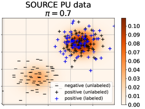
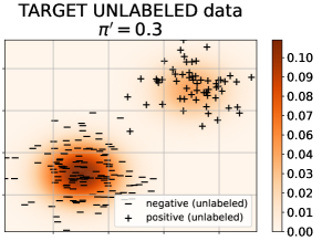
Figure 1: Label shift visualization for PU data. Source (training) data contains positive (blue) and unlabeled (grey) observations. Target (test) data contains only unlabeled observations. Class priors differ between target ($\pi=0.7$) and source data ($\pi^{\prime}=0.3$). The goal is to estimate target class prior $\pi^{\prime}$ using source PU data and target unlabeled data.

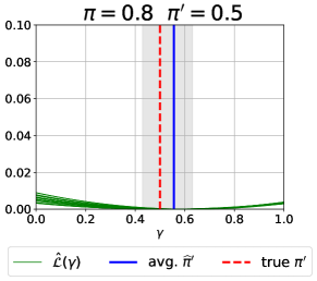
Figure 2: Visualization of the objective function behavior for $\pi$=0.2, 0.8 and $\pi^{\prime}=0.5$. The TCPU estimator is defined as $\widehat{\pi}^{\prime}=\arg\min_{\gamma}\hat{\mathcal{L}}(\gamma)$. The grey area indicates the range of estimator’s values for $20$ runs. For larger $\pi$, the objective function is flat and has a less pronounced minimum.

2 Label shift for positive unlabeled learning

We first introduce relevant notation. Let $X\in{\cal X}$ be a random variable corresponding to a feature vector, $Y\in\{-1,1\}$ be a true class indicator and $P_{XY}$ their joint distribution (called a source distribution). We consider a problem of modeling Positive Unlabeled data in case-control setting, which means that only samples coming from the positive class and samples coming from the overall population $X$ are available. More formally, let $P_{X}$ be the distribution of $X$ and $P_{+}=P_{X|Y=1}$, $P_{-}=P_{X|Y=-1}$ the distributions of samples from the positive class and the negative class, respectively. We denote by $X_{1},\ldots,X_{n}$ independent samples generated according to $P_{X}$ and $X_{1}^{+},\ldots,X_{m}^{+}$ generated according to $P_{+}$.

Moreover, we consider the second vector $(X^{\prime},Y^{\prime})$ such that its distribution $P^{\prime}_{X^{\prime}Y^{\prime}}$ (called a target distribution) is a label shifted distribution of $(X,Y)$, which means that the marginal distribution of $Y^{\prime}$ is different from that of $Y$, i.e.

$$\pi^{\prime}=P(Y^{\prime}=1)\neq P(Y=1)=\pi,$$

however, the covariate distributions in both the positive and the negative class remain the same:

$$P^{\prime}_{X^{\prime}|Y^{\prime}=i}=P_{X|Y=i}\quad{\rm for}\quad i=\pm 1.$$

Thus, we have that a distribution of $X^{\prime}$ satisfies $P^{\prime}_{X^{\prime}}=\pi^{\prime}P_{+}+(1-\pi^{\prime})P_{-}$ and is different from $P_{X}=\pi P_{+}+(1-\pi)P_{-}$.

Denote by $X_{1}^{\prime},\ldots,X_{n^{\prime}}^{\prime}$ independent samples generated from $P^{\prime}_{X^{\prime}}$. In the paper we consider the problem of estimation of label-shifted probability $\pi^{\prime}$. Note that that the problem is nontrivial as the class indicators corresponding to shifted samples are not available. However, we have at our disposal data from the positive class and unlabeled $X$ observations corresponding to a different prior $\pi$.

We note that if $\pi$ is known the distribution $P_{-}$ is uniquely determined and the problem is well defined in general. When $\pi$ is unknown, the specific assumptions are needed under which it is identifiable, e.g. an assumption that $P_{-}$ is not a convex combination of $P_{+}$ and other probability measure (see e.g. [25]). We stress that identifiability is necessary to investigate theoretical properties of considered estimate.

Finally, it is worth mentioning that the estimation of $\pi^{\prime}$ is crucial to define a classification rule for the target set which involves a modified threshold base on $\pi^{\prime}$, see e.g. [19].

3 Class prior estimation for target data

3.1 TCPU: a novel kernel-based estimator of class prior

In this section we introduce a novel method of estimating $\pi^{\prime}$, which will be called TCPU (Target Class prior estimator for Positive-Unlabled data under label shift).

Let $K(\cdot,\cdot)$ be a kernel function (i.e. symmetric, continuous and semi-positive function defined on $\cal X\times\cal X$) and let $\cal H$ be a Reproducing Kernel Hilbert Space (RHKS) induced by $K(\cdot,\cdot)$ (see e.g. [8]). We denote an associated kernel transform by $\phi(x)=K(x,\cdot)\in{\cal H}.$ From the reproducing property $<f,\phi(x)>_{\cal H}=f(x)$ for each $x\in{\cal X},f\in\cal H$ and a scalar product in $\cal H$ is defined by a kernel as $<\phi(x_{1}),\phi(x_{2})>_{\cal H}=K(x_{1},x_{2})$ for each $x_{1},x_{2}\in\cal X$ and extending it for general elements of ${\cal H}$. Next, let $\Phi(P_{X})=\mathbbm{E}\phi(X)=\int_{\cal X}\phi(s)\,P_{X}(ds)\in{\cal H}$ be a mean functional of $P_{X}$ with a norm $||\Phi(P_{X})||_{\cal H}^{2}=\mathbbm{E}K(X_{1},X_{2}),$ where $X_{1}$ and $X_{2}$ are two independent random vectors following a distribution $P_{X}.$ The mean functionals $\Phi(P_{+})$ and $\Phi(P^{\prime}_{X^{\prime}})$ are defined analogously. Recall that when kernel is universal we have that $\Phi(P)=\Phi(Q)$ is equivalent to the fact that distributions $P$ and $Q$ coincide [8].

Let $\hat{P}_{X}$, $\hat{P}_{+}$ and $\hat{P^{\prime}}_{X^{\prime}}$ be empirical distributions corresponding to observable samples. In the following we will omit indices $X$ and $X^{\prime}$ in $P_{X}$ and $P^{\prime}_{X^{\prime}}$, respectively, and the same convention is applied to their empirical counterparts. We note that due to the fact that $\hat{P}$ is a discrete distribution with mass $n^{-1}$ at each observation $X_{i}$ we have that $\Phi(\hat{P})=n^{-1}\sum_{i=1}^{n}\phi(X_{i})$ and analogous representations hold for $\Phi(\hat{P}_{+})$ and $\Phi(\hat{P}^{\prime})$.

In the above setup we have that

$$(1-\pi^{\prime})(P-\pi P_{+})=(1-\pi^{\prime})(1-\pi)P_{-}=(1-\pi)(P^{\prime}-\pi^{\prime}P_{+}).$$

Therefore, in order to determine $\pi^{\prime}$, it is natural to substitute $\gamma$ for $\pi^{\prime}$ and minimize the following objective function

$$\mathcal{L}(\gamma)=||(1-\gamma)[\Phi(P)-\pi\Phi(P_{+})]-(1-\pi)[\Phi(P^{\prime})-\gamma\Phi(P_{+})]||^{2}_{\cal H}.$$ (1)

Lemma 1

Suppose that a kernel $K$ is universal, $P_{+}\neq P_{-}$ and $\pi<1$. Then $\pi^{\prime}$ is unique minimizer of $\mathcal{L}(\gamma)$.

Proof

Denote by $Crit(\gamma)$ the function given by

$$Crit(\gamma)=|\pi^{\prime}-\gamma|\times(1-\pi)||\Phi(P_{-})-\Phi(P_{+})||_{\cal H}.$$ (2)

Then by noting that

$$\Phi(P)-\pi\Phi(P_{+})=(1-\pi)\Phi(P_{-}),\quad\quad\Phi(P^{\prime})-\gamma\Phi(P_{+})=(\pi^{\prime}-\gamma)\Phi(P_{+})+(1-\pi^{\prime})\Phi(P_{-})$$

we have that $\mathcal{L}(\gamma)=[Crit(\gamma)]^{2}$ and the minimiser of $Crit(\gamma)$ is obviously $\pi^{\prime}$.

In the proposed method, we consider the empirical version of (1) given as

$$\widehat{\mathcal{L}}(\gamma)=||(1-\gamma)[\Phi(\hat{P})-\pi\Phi(\hat{P}_{+})]-(1-\pi)[\Phi(\hat{P^{\prime}})-\gamma\Phi(\hat{P}_{+})]||^{2}_{\cal H}$$ (3)

and the estimator of $\pi^{\prime}$ is defined as its minimizer

$$\widehat{\pi}^{\prime}={\rm argmin}_{\gamma}\widehat{\mathcal{L}}(\gamma).$$ (4)

The estimator defined above will be called TCPU further on. For theoretical results it will be assumed that $\pi$ is known. This assumption is plausible when the large data base corresponding to source distribution is available. In the experiments we estimate $\pi$ using well-known KM2 method [25] and then plug-in it into (3). Note that the slope of $Crit(\gamma)$ is proportional to $1-\pi$ and close to 0 for $\pi\approx 1.$ It will make estimation of $\pi^{\prime}$ more difficult for large $\pi$.

In the following lemma we show that the proposed estimator can be explicitly calculated using a simple algebraic formula.

Lemma 2

Let $\widehat{\pi}^{\prime}$ be defined by (4). Then we have

$$\widehat{\pi}^{\prime}=\frac{<\Phi(\hat{P})-\Phi(\hat{P}_{+}),\Delta>_{\cal H}}{||\Phi(\hat{P})-\Phi(\hat{P}_{+})||_{\cal H}^{2}}=1-\frac{(1-\pi)<\Phi(\hat{P})-\Phi(\hat{P}_{+}),\Phi(\hat{P^{\prime}})-\Phi(\hat{P}_{+})>_{\cal H}}{||\Phi(\hat{P})-\Phi(\hat{P}_{+})||_{\cal H}^{2}},$$ (5)

where $\Delta=\Phi(\hat{P})-\pi\Phi(\hat{P}_{+})-(1-\pi)\Phi(\hat{P^{\prime}}).$

Remark 1

In view of the first equality in (5), $\widehat{\pi}^{\prime}$ has a simple geometric interpretation: it is a coefficient of projection of $\Delta$ on $\Phi(\hat{P})-\Phi(\hat{P}_{+})$ in ${\cal H}$.

Proof

Simple calculations show that the expression under the norm in (3) equals

$$-\gamma[\Phi(\hat{P})-\Phi(\hat{P}_{+})]+\Phi(\hat{P})-\pi\Phi(\hat{P}_{+})-(1-\pi)\Phi(\hat{P^{\prime}})=-\gamma[\Phi(\hat{P})-\Phi(\hat{P}_{+})]+\Delta.$$

Thus, the squared norm equals

$$\gamma^{2}||\Phi(\hat{P})-\Phi(\hat{P}_{+}))||_{\cal H}^{2}+2\gamma<\Phi(\hat{P}_{+})-\Phi(\hat{P}),\Delta>_{\cal H}+||\Delta||_{\cal H}^{2}$$

and the first form of $\widehat{\pi}^{\prime}$ follows by calculating a minimizer of the above function. The second formula follows by simple algebraic manipulations.

The kernel approach is a core of Maximum Mean Discrepancy (MMD) method which matches the distributions based on the features in RHKS induced by kernel $K$. It is frequently used in machine learning and statistics to compare a data distribution with a specific distribution, in a two sample problem and covariate shift detection (see [13]). It has been also applied for the label shift problem in classical framework. Namely, for the case when distribution $P_{XY}$ is observable the approach relies on the equality (cf [31])

$$\pi^{\prime}={\rm argmin}_{\lambda\in[0,1]}\quad||\Phi(P_{X^{\prime}})-[\lambda\Phi(P_{+})+(1-\lambda)\Phi(P_{-})]||^{2}_{\cal H}$$ (6)

(see also [14] and [5]). In the considered scenario, a direct application of (6) to estimate $\pi^{\prime}$ is clearly infeasible, as observations from the negative class are not available. The estimator (4) can be considered as a modification for the MMD approach applied for label shift in PU setting.
In numerical experiments we will also consider a modified TCPU estimator, called TCPU+, which switches from TCPU to KM2-LS defined in Section 4.2 below, when denominator in (5) falls below a predefined threshold. Note that $||\Phi(P)-\Phi(P_{+})||_{\cal H}$ is proportional to $(1-\pi)$ and it is expected, in view of the discussion above, that performance of TCPU will deteriorate for large $\pi$. In Figure 2 we visualise the essence of the problem. For large $\pi$ the objective function $\hat{\cal L}(\gamma)$ is flat around its minimum and thus $\widehat{\pi}^{\prime}$ is less accurate than for smaller $\pi$.

3.2 Asymptotic consistency and non-asymptotic error bounds for the proposed estimator

We let $N=\min(n,m,n^{\prime})$. In the next result we establish asymptotic and nonasymptotic error bounds for $\widehat{\pi}^{\prime}.$ We also state conditions, which guarantee that $||\Phi(\hat{P})-\Phi(\hat{P}_{+})||_{\cal H}>0,$ which is implicitly assumed in (5).

Theorem 3.1

Suppose that a kernel $K$ is universal, $P_{+}\neq P_{-}$ and $\pi<1.$
(i) Moreover, assume $\mathbbm{E}K(X,X)<\infty$ for $X\sim P$ and analogous conditions hold for $X^{+}\sim P_{X|Y=1}$ and $X^{\prime}\sim P^{\prime}$. Then for $N\to\infty$ we have $\hat{\pi}^{\prime}\to\pi^{\prime}$ in probability.
(ii) Assume that $M=\sup_{x}K(x,x)<\infty.$ Moreover, fix $\alpha\in(0,1)$ and $\delta\leq\exp(-(\sqrt{2}+1)^{2}/2)$ and let

$$N\geq\frac{16M\log(1/\delta)}{(1-\alpha)^{2}(1-\pi)^{2}||\Phi(P_{-})-\Phi(P_{+})||^{2}_{\cal H}}\;.$$ (7)

Then we have

$$P\left(|\widehat{\pi}^{\prime}-\pi^{\prime}|\leq\frac{4\sqrt{\frac{M}{N}\log(1/\delta)}}{\alpha(1-\pi)||\Phi(P_{-})-\Phi(P_{+})||_{\cal H}}\right)\geq 1-3\delta.$$ (8)

We note that consistency of $\widehat{\pi}^{\prime}$ is proved in Theorem 3.1(i) under weak conditions. Indeed, dropping the conditions $P_{+}\neq P_{-}$ and $\pi\neq 1$ makes the problem ill-posed. Finally, the restrictions imposed on a kernel are satisfied, for instance, for a gaussian kernel.

The claim of Theorem 3.1 (ii) is stronger (it is an nonasymptotic result implying asymptotic consistency), so it needs more restrictive assumptions as well. However, these conditions are reasonable as in (i). For instance, a gaussian kernel satisfies the assumption in (ii) with $M=1.$ The dependence of an error bound on $N,\delta,\pi,||\Phi(P_{-})-\Phi(P_{+})||_{\cal H}$ is stated explicitly in (8). Clearly, an error of $\widehat{\pi}^{\prime}$ decreases as $N$ increases. Also, as it should be expected, the bound for $|\widehat{\pi}^{\prime}-\pi^{\prime}|$ increases when $P_{+}$ gets closer to $P_{-}$ or $\pi$ increases. Finally, note that the condition on $N$ in (7) becomes more restrictive for increasing $\pi$.

Theorem 3.2

Assume that $M=\sup_{x}K(x,x)<\infty.$ Then for any $\delta\leq\exp(-(\sqrt{2}+1)^{2}/2)$ we have that

$$P\left(|\widehat{\pi}^{\prime}-\pi^{\prime}|\leq\frac{4\sqrt{\frac{M}{N}\log(1/\delta)}}{||\Phi(\hat{P})-\Phi(\hat{P}_{+})||_{\cal H}}\right)\geq 1-3\delta.$$ (9)

We stress the differences between Theorems 3.2 and 3.1. Probability inequality (9) does not require assumption (7) and it yields a bound on an estimation error which depends on $||\Phi(\hat{P})-\Phi(\hat{P}_{+})||_{\cal H}.$ Notice that this bound can be calculated in practice. On the other hand, the error bound in (8) is nonrandom and explicitly establishes the dependence on $\pi$ and a distance between $P_{-}$ and $P_{+}.$

Proof (of Theorem 3.1)

The proof of (i) follows from Chebyshev’s inequality applied for $\Phi(\hat{P})=n^{-1}\sum_{i=1}^{n}\Phi(X_{i})$ as well as $\Phi(\hat{P}_{+})$ and $\Phi(\hat{P}^{\prime})$: fix $\varepsilon>0$, then

$$P(||\Phi(\hat{P})-\Phi(P)||_{\cal H}>\varepsilon)\leq\frac{\mathbbm{E}||\Phi(\hat{P})-\Phi(P)||^{2}_{\cal H}}{\varepsilon^{2}}.$$ (10)

Now we focus on bounding the numerator in (10). First, we obtain

$$\mathbbm{E}||\Phi(\hat{P})-\Phi(P)||^{2}=\mathbbm{E}||\Phi(\hat{P})||^{2}_{\cal H}-2\mathbbm{E}<\Phi(\hat{P}),\Phi(P)>_{\cal H}+||\Phi(P)||^{2}_{\cal H}.$$ (11)

Next, we consider the two first terms on the right-hand side of (11). For the first one, we have:

$$\mathbbm{E}\left|\left|\frac{1}{n}\sum_{i=1}^{n}\phi(X_{i})\right|\right|^{2}_{\cal H} = \frac{1}{n^{2}}\sum_{i=1}^{n}\sum_{j=1}^{n}<\phi(X_{i}),\phi(X_{j})>_{\cal H}=\frac{1}{n^{2}}\sum_{i=1}^{n}\sum_{j=1}^{n}K(X_{i},X_{j})$$

$$= \frac{1}{n^{2}}\sum_{i=1}^{n}\mathbbm{E}K(X_{i},X_{i})+\frac{1}{n^{2}}\sum_{1\leq i\neq j\leq n}\mathbbm{E}K(X_{i},X_{j})$$

$$= \frac{1}{n}\mathbbm{E}K(X_{1},X_{1})+\left(1-\frac{1}{n}\right)||\Phi(P)||^{2}_{\cal H}.$$

Moreover, we have

$$\mathbbm{E}<\Phi(\hat{P}),\Phi(P)>_{\cal H}=\frac{1}{n}\sum_{i=1}^{n}\mathbbm{E}<\phi(X_{i}),\Phi(P)>_{\cal H}=\mathbbm{E}<\phi(X_{1}),\Phi(P)>_{\cal H}.$$ (12)

From the reproducing property we obtain $<\phi(x_{1}),\Phi(P)>_{\cal H}=[\Phi(P)](x_{1})=\mathbbm{E}K(X,x_{1}).$ Therefore, the right-hand side of (12) equals $||\Phi(P)||^{2}_{\cal H}.$ Finally, (11) is $\frac{1}{n}[\mathbbm{E}K(X,X)-||\Phi(P)||^{2}_{\cal H}],$ so the right-hand side of (10) tends to zero as $n$ goes to infinity. This fact implies that $\Phi(\hat{P})$ tends to $\Phi(P)$ in probability. Obviously, the analogous properties hold for $\Phi(\hat{P}_{+})$ and $\Phi(\hat{P}^{\prime})$. In particular, we have that $||\Phi(\hat{P})-\Phi(\hat{P}_{+})||_{\cal H}$ is positive with probability tending to one as $N\to\infty$. It follows from continuity of a norm and the assumptions

$$||\Phi(\hat{P})-\Phi(\hat{P}_{+})||_{\cal H}\to_{P}||\Phi(P)-\Phi(P_{+})||_{\cal H}=(1-\pi)||\Phi(P_{-})-\Phi(P_{+})||_{\cal H}.$$

Thus, the second equality in (5) and continuity of a scalar product give

$$\hat{\pi}^{\prime}\to_{P}\quad 1-\frac{(1-\pi)<\Phi(P)-\Phi(P_{+}),\Phi({P^{\prime}})-\Phi({P_{+}})>_{\cal H}}{||\Phi(P)-\Phi({P_{+}})||_{\cal H}^{2}}=\pi^{\prime}.$$

Next, we focus on the proof of (ii). From the first equality in (5) and the Cauchy–Schwarz inequality we have

$$|\widehat{\pi}^{\prime}-\pi^{\prime}| =\frac{<\Phi(\hat{P})-\Phi(\hat{P}_{+}),\Delta-\pi^{\prime}[\Phi(\hat{P})-\Phi(\hat{P}_{+})]>_{\cal H}}{||\Phi(\hat{P})-\Phi(\hat{P}_{+})||_{\cal H}^{2}}$$ (13)

$$\leq\frac{||\Delta-\pi^{\prime}[\Phi(\hat{P})-\Phi(\hat{P}_{+})]||_{\cal H}}{||\Phi(\hat{P})-\Phi(\hat{P}_{+})||_{\cal H}}.$$

Notice that

$$\Delta-\pi^{\prime}[\Phi(\hat{P})-\Phi(\hat{P}_{+})]=(1-\pi^{\prime})\Phi(\hat{P})-(1-\pi)\Phi(\hat{P}^{\prime})+(\pi^{\prime}-\pi)\Phi(\hat{P}_{+})$$

and

$$(1-\pi^{\prime})\Phi(P)-(1-\pi)\Phi(P^{\prime})+(\pi^{\prime}-\pi)\Phi(P_{+})=0,$$

which imply that

$$||\Delta-\pi^{\prime}[\Phi(\hat{P})-\Phi(\hat{P}_{+})]||_{\cal H}\leq(1-\pi^{\prime})||\Phi(\hat{P})-\Phi(P)||_{\cal H}$$

$$+(1-\pi)||\Phi(\hat{P}^{\prime})-\Phi(P^{\prime})||_{\cal H}+|\pi^{\prime}-\pi|\times||\Phi(\hat{P}_{+})-\Phi(P_{+})||_{\cal H}.$$

Now we use Lemma 3 (given below) and consider the event on which all three inequalities in this lemma hold. In this case

$$||\Delta-\pi^{\prime}[\Phi(\hat{P})-\Phi(\hat{P}_{+})]||_{\cal H}\leq 4\sqrt{\frac{M}{N}\log(1/\delta)}$$ (14)

and

$$||\Phi(\hat{P})-\Phi(\hat{P}_{+})||_{\cal H}\geq||\Phi(P)-\Phi(P_{+})||_{\cal H}-||\Phi(\hat{P})-\Phi(P)||_{\cal H}-||\Phi(\hat{P}_{+})-\Phi(P_{+})||_{\cal H},$$

which again can be bounded by

$$(1-\pi)||\Phi(P_{-})-\Phi(P_{+})||_{\cal H}-4\sqrt{\frac{M}{N}\log(1/\delta)}.$$

From the assumption (7) the above expression is not smaller than $\alpha(1-\pi)||\Phi(P_{-})-\Phi(P_{+})||_{\cal H}.$ In particular, we have that $||\Phi(\hat{P})-\Phi(\hat{P}_{+})||_{\cal H}$ is positive with high probability. Since the numerator and the denominator on the right-hand side of (13) are bounded, the proof of (ii) is finished.

Proof (of Theorem 3.2)

The proof is even simpler than the proof of Theorem 3.1 and involves bounding the numerator on the RHS of (13) done in (14).

Lemma 3

Suppose that $M=\sup_{x}K(x,x)<\infty$ and $\delta\leq\exp(-(\sqrt{2}+1)^{2}/2)$ is arbitrary. Then with probability at least $1-3\delta$ the following three inequalities simultaneously hold

$$||\Phi(\hat{P})-\Phi(P)||_{\cal H}\leq 2\sqrt{\frac{M}{n}\log(1/\delta)}\>, ||\Phi(\hat{P}^{\prime})-\Phi(P^{\prime})||_{\cal H}\leq 2\sqrt{\frac{M}{n^{\prime}}\log(1/\delta)}\>,$$

$$||\Phi(\hat{P}_{+})-\Phi(P_{+})||_{\cal H}\leq 2\sqrt{\frac{M}{m}\log(1/\delta)}\>.$$

The similar concentration inequalities are proven, for instance, in [29, Proposition A.1 and Remark A.2]. For completeness we provide the proof in supplementary material.

4 Related work

4.1 Method DRPU

The most related method is DRPU [22], which in the label-shift setting considered here, constructs empirical Bayes classifier for samples from label shifted population. It involves estimator of ratio $r$ of densities of distributions $P_{+}$ and $P$ for training data and of both prior probabilities $\pi$ and $\pi^{\prime}$. Estimator $\hat{r}$ of $r$ is a minimiser of expected Bregman divergence functional (cf Section 2.5 in [22]) and both prior estimators are based on an observation (cf [3]) that $\pi$ and $\pi^{\prime}$ can be recovered in PU setting by minimising $P(A)/P_{+}(A)$ (respectively $P^{\prime}(A)/P_{+}(A)$) over all sets $A$ for which $P_{+}(A)>0$. In [22] ratio $\hat{P}^{\prime}(A)/\hat{P}_{+}(A)$ is minimised over sets being the level sets of $\hat{r}$. The estimator based on the above method will be denoted simply as DRPU.

4.2 Adapting the KM method to label shift

The popular KM [25] method of estimating the prior in PU setting can be straightforwardly modified in order to account for label shift. [25] is based on the observation that distribution of negative class $P_{-}$ can be written as $P_{-}=\lambda P+(1-\lambda)P_{+}$, where $\lambda=1/(1-\pi)$ and thus, analogously to (6), estimator of $\lambda$ can be constructed by projecting $\gamma\Phi(P)+(1-\gamma)\Phi(P_{+})$ on a convex $\mathcal{C}$ hull of $\phi(X_{1}),\ldots,\phi(X_{n}),\phi(X_{1}^{+}),\ldots,\phi(X_{m}^{+})$ and defining $\hat{\lambda}$ as $\gamma$ yielding the smallest distance. This leads to two estimators of $\pi$, KM1 and KM2 investigated in [25]. As unavailable positive samples for test population have the same distribution as positive observations from training distribution, we can apply approach from [25] to samples $X^{\prime}_{1},\ldots,X^{\prime}_{n^{\prime}},X_{1}^{+},\ldots,X_{m}^{+}$ and obtain KM2 estimator of $\pi^{\prime}$ also investigated below. The adaptation will be called KM2-LS in the following.

5 Experiments

5.1 Methods

We empirically evaluate the effectiveness of TCPU and TCPU+ to recover the true target class prior $\pi^{\prime}$. As baselines we used DRPU [22] and KM2-LS methods described in Section 4. In the case of DRPU, we used the implementation made publicly available by the authors. In the case of KM2-LS, we used the code of the standard KM2 method [25] and adopted it to our setting as described in Section 4. Note that TCPU and TCPU+ require knowledge of $\pi$. Since typically, $\pi$ remains unknown, we estimate it using KM2 estimator [25] for both methods. Importantly, the KM2-LS method does not require the $\pi$ estimation. The DRPU method is the only one that requires learning a parametric model. As in the original work, we used MLP to this end. Due to space constraints, technical details about the model used in DRPU and the selection of hyperparameters are discussed in the supplement (Section 5).

For TCPU, we used Gaussian kernel $K(x,y)=\exp(-\tau||x-y||^{2})$ with the default value of parameter $\tau=1/p$, where $p$ is the number of features. We also consider TCPU+ discussed at the end of Section 3.1, which switches from TCPU to KM2-LS if the $||\Phi(\hat{P})-\Phi(\hat{P}_{+})||_{\cal H}<s$, where $s$ is a threshold. The value of $s=0.02$ was empirically chosen based on examination of performance of TCPU.

5.2 Datasets

The experiments were conducted on 10 datasets, including one synthetic dataset, 6 tabular datasets from the UCI repository (Diabetes, Spambase, Segment, Waveform, Vehicle, Yeast), and 3 image datasets: CIFAR-10, MNIST, and FashionMNIST [23]. For the synthetic dataset, negative observations are generated from a 10-dimensional normal distribution $N(0,I)$, and positive observations are generated from $N(a,I)$, where $a=(1,\ldots,1)$. The characteristics of the UCI and image datasets are provided in the supplement. Tabular datasets with multiple classes were transformed into binary classification datasets, where the most common class is treated as the positive class, and the remaining classes are combined into the negative class. For image datasets, the binary class variable is defined according to the specific dataset, following methods used in other PU learning papers [16, 11, 22]. For MNIST, even digits form the positive class, and odd digits form the negative class. In CIFAR-10, vehicles form the positive class, and animals form the negative class. For FashionMNIST, clothing items worn on the upper body are marked as positive cases, and the remaining items are assigned to the negative class. For image data, we use a pre-trained deep neural network, ResNet18, to extract the feature vector. For each image, the feature vector, with a dimension of 512, is the output of the average pooling layer. From the extracted 512-dimensional feature vector, we select the 30 most correlated features with the class variable to reduce the dimensionality of the problem.

5.3 Experimental settings

First, each dataset is split into a source and a target dataset. For image data, we use the splits defined in the PyTorch library [23]. For synthetic datasets, we generate observations for fixed values of $\pi$ and $\pi^{\prime}$. For real datasets, we simulate a label shift scenario using the downsampling technique. Specifically, we randomly remove observations from one of the classes in both the source and target datasets to control the class priors $\pi$ and $\pi^{\prime}$, respectively. Finally, based on the source data, we artificially create a PU dataset by selecting some positive observations for the labeled subset, while the unlabeled subset consists of a mixture of positive and negative observations. We follow the procedure described in [21] to control the size of the source data and the labeling frequency $c$, which represents the percentage of labeled observations among all positive observations. In the experiments, we set $c=0.5$. The entire target dataset is treated as unlabeled. The considered methods take as input the source PU data and unlabeled target data. For each method, we calculate the absolute estimation error $|\pi^{\prime}-\widehat{\pi}^{\prime}|$, where $\widehat{\pi}^{\prime}$ is the estimator returned by the method. We perform 20 repetitions of the above procedure and analyze the distributions of the errors.

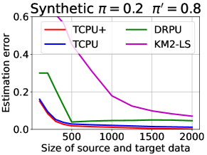
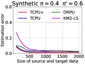
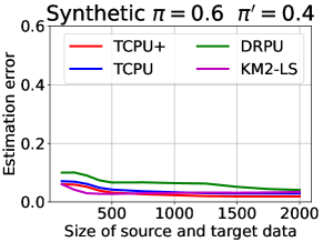
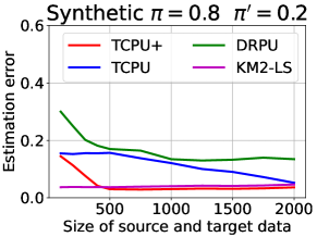
Figure 3: Estimation errors wrt size of data.

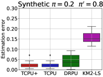
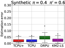
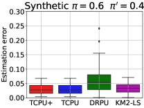
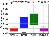
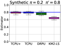
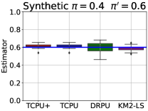
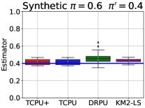
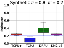
Figure 4: Rows 1, 2: distribution of estimation errors and distribution of estimators (blue line indicates the true $\pi^{\prime}$). Size of the source data and the target data is $1000$.

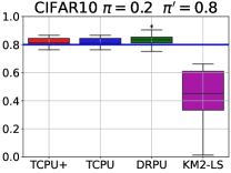
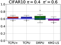
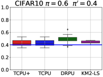
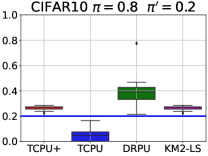
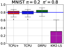
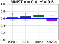
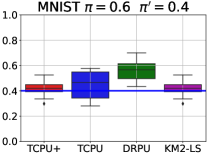
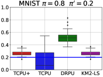
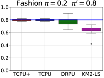
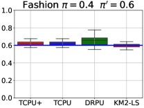
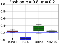
Figure 5: Distribution of estimators for image datasets. Blue line indicates true $\pi^{\prime}$.

5.4 Discussion

Figures 3, 4, 5, and 6 show the distributions of estimators and estimation errors for the analyzed datasets. Additional results for synthetic and image data are also provided in the supplement (Sections 3-5). Since our primary interest lies in analyzing estimation errors for small or moderate data samples, we present the boxplots for the case where the source and target datasets consist of randomly chosen samples of 1000 observations. When the total number of observations in the original dataset is less than 2000, we split the data into source and target datasets in equal proportions. Experiments indicate that the values of $\pi$ and $\pi^{\prime}$ significantly influence the quality of the $\pi^{\prime}$ estimation, with the impact differing across methods. For the TCPU method, we observe small estimation errors for small or moderate values of $\pi=0.2,0.4,0.6$, regardless of the value of $\pi^{\prime}$. However, for $\pi=0.8$, the errors for TCPU increase. This is likely due to the issue of the lack of a well-pronounced minimum for the objective function, as discussed at the end of Section 3.1 and illustrated in Figure 2. In this case, TCPU underestimates the true $\pi^{\prime}$. This problem is avoided in the TCPU+ method, which is highly effective for all values of $\pi$. In the problematic situation occurring for large $\pi$, TCPU+ switches from TCPU to KM2-LS. However, the KM2-LS method itself performs significantly worse than competing methods for small $\pi$, due to the underestimation of the true value of $\pi^{\prime}$. The DRPU method produces large estimation errors for $\pi=0.8$, which is related to the overestimation of $\pi^{\prime}$. The effect of dataset size on the quality of the estimation is shown in Figure 4 (row 1). Additional figures in the supplement illustrate the individual effects of variable source and target dataset sizes. For $\pi=0.2$, the estimation error for the DRPU method diminishes much more slowly than for the other methods. In this case, DRPU yields large errors for small sample sizes, which decrease as the sample size increases. On the other hand, for $\pi=0.8$, large errors are observed for DRPU, regardless of dataset size. TCPU+ can be recommended as a method that performs consistently well across all considered combinations of $\pi$ and $\pi^{\prime}$ values.

It is worth noting that DRPU is the only method considered that requires model training, which leads to longer computation times (see Section 7 in the supplement). For example, for image datasets, TCPU is about 4–6 times faster than DRPU for $\pi=0.2$ and $\pi=0.8$, respectively. The computational times for TCPU and TCPU+ are the same for $\pi=0.2$, whereas for $\pi=0.8$, TCPU+ runs slower than TCPU due to the additional time required to determine the threshold for the switch between TCPU and KM2-LS, as well as the execution time of the KM2-LS method itself.

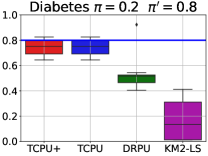
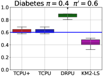
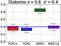
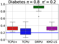
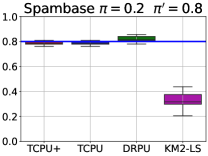
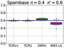
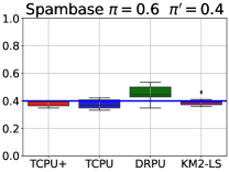
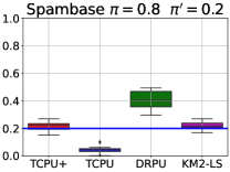
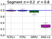
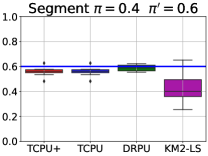
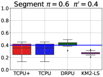
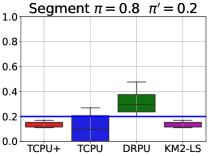
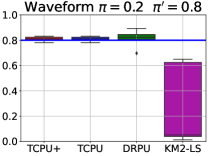
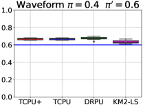
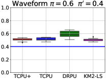
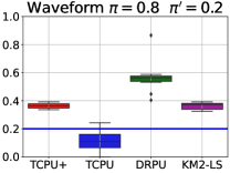
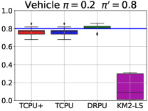
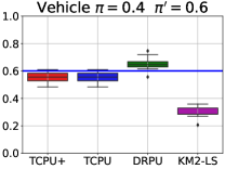
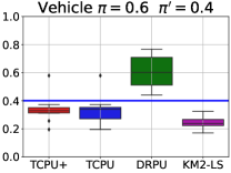
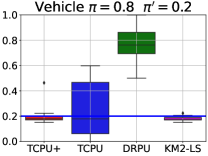
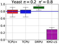
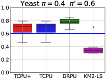
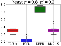
Figure 6: Distribution of estimators for benchmark datasets.

6 Conclusions and future work

In this paper, we introduced a novel estimator, TCPU, for estimating the target class prior $\pi^{\prime}$ under label shift in the context of positive-unlabeled (PU) learning. Our approach, which leverages distribution matching and kernel embedding, provides an explicitly expressed estimate of the target class prior without estimating posterior probabilities via classifier training. We proved that the TCPU estimator is both asymptotically consistent and established a calculable non-asymptotic error bound. Experimental results on synthetic and real datasets show that TCPU outperforms or performs on par with existing methods, particularly in cases of moderate source class prior $\pi$ values. In situations where larger values of $\pi$ cause TCPU to underestimate the target class prior, the TCPU+ variant effectively mitigates this issue by switching to the KM2-LS method when necessary. A natural direction for future research is to further investigate the effect of $\pi$ and $\pi^{\prime}$ estimation on classification accuracy and to develop methods checking whether label-shift occurs. Also, generalisation of the proposed method to not necessarily binary nominal response Y by considering extension of PU scenario to noisy data model ([32]) is of interest.

References

- [1] Bekker, J., Davis, J.: Estimating the class prior in positive and unlabeled data through decision tree induction. In: Proceedings of the 32th AAAI Conference on Artificial Intelligence. pp. 1–8 (2018)
- [2] Bekker, J., Davis, J.: Learning from positive and unlabeled data: a survey. Machine Learning 109, 719–760 (2020)
- [3] Blanchard, G., Lee, G., Scott, C.: Semi-supervised novelty detection. Journal of Machine Learning Research 11, 2973–3009 (2010)
- [4] Chen, X., Chen, W., Chen, T., Yuan, Y., Gong, C., Chen, K., Wang, Z.: Self-PU: Self boosted and calibrated positive-unlabeled training. In: Proceedings of the 37th International Conference on Machine Learning. ICML’20 (2020)
- [5] Dussap, B., Blanchard, G., Chérif-Abdellatif, B.E.: Label shift quantification with robustness guarantees via distribution feature matching. In: Proceedings of the European Conferencce on Machine Learning (2023)
- [6] Elkan, C., Noto, K.: Learning classifiers from only positive and unlabeled data. In: Proceedings of the 14th ACM SIGKDD International Conference on Knowledge Discovery and Data Mining. pp. 213–220. KDD ’08 (2008)
- [7] Forman, G.: Quantifying counts and costs via classification. Data Mining and Knowledge Discovery 17, 164–206 (2008)
- [8] Fukumizu, K., Gretton, A., Sun, X., Schölkopf, B.: Kernel measures of conditional dependence. In: Advances in Neural Information Processing Systems. vol. 20 (2007)
- [9] Fung, G.P.C., Yu, J.X., Lu, H., Yu, P.S.: Text classification without negative examples revisit. IEEE Transactions on Knowledge and Data Engineering 18(1), 6–20 (2006)
- [10] Garg, S., Wu, Y., Balakrishnan, S., Lipton, Z.C.: A unified view of label shift estimation. In: Proceedings of the 34th International Conference on Neural Information Processing Systems. pp. 1–11. NIPS’ 20 (2020)
- [11] Gong, C., Wang, Q., Liu, T., Han, B., You, J., Yang, J., Tao, D.: Instance-dependent positive and unlabeled learning with labeling bias estimation. IEEE Trans Pattern Anal Mach Intell pp. 1–16 (2021)
- [12] González, P., Castaño, A., Chawla, N., Coz, J.: A review on quantification learning. ACM Comput. Surv. 50(5) (2017)
- [13] Gretton, A., Borgwardt, K., Rasch, M., Schölkopf, B., Smola, A.: A kernel two-sample test. Journal of Machine Learning Research 13, 723–773 (2012)
- [14] Iyer, A., Nath, S., Sarawagi, S.: Maximum mean discrepancy for class ratio estimation: convergence bounds and kernel selection. In: Proceedings of the 31th International Conferencce on Machine Learning. IMLR W & CP vol. 32 (2014)
- [15] Jain, S., White, M., Radivojac, P.: Estimating the class prior and posterior from noisy positives and unlabeled data. In: Proceedings of the 30th International Conference on Neural Information Processing Systems. p. 2693–2701 (2016)
- [16] Kiryo, R., Niu, G., du Plessis, M.C., Sugiyama, M.: Positive-unlabeled learning with non-negative risk estimator. In: Proceedings of the International Conference on Neural Information Processing Systems. pp. 1674–1684. NIPS’17 (2017)
- [17] Li, F., Dong, S., Leier, A., Han, M., Guo, X., Xu, J., Wang, X., Pan, S., Jia, C., Zhang, Y., Webb, G., Coin, L.J.M., Li, C., Song, J.: Positive-unlabeled learning in bioinformatics and computational biology: a brief review. Briefings in Bioinformatics 23(1) (2021)
- [18] Li, X., Liu, B.: Learning to classify texts using positive and unlabeled data. In: Proceedings of the 18th International Joint Conference on Artificial Intelligence. p. 587–592. IJCAI’03 (2003)
- [19] Lipton, Z.C., Wang, Y., Smola, A.J.: Detecting and correcting for label shift with black box predictors. In: Proceedings of the 35th International Conference on Machine Learning. pp. 3128–3136. ICML’ 18 (2018)
- [20] Luo, C., Zhao, P., Chen, C., Qiao, B., Du, C., Zhang, H., Wu, W., Cai, S., He, B., Rajmohan, S., Lin, Q.: Pulns: Positive-unlabeled learning with effective negative sample selector. In: Proceedings of the AAAI Conference on Artificial Intelligence. AAAI’21, vol. 35, pp. 8784–8792 (2021)
- [21] Mielniczuk, J., Wawrzeńczyk, A.: Single-sample versus case-control sampling scheme for Positive Unlabeled data: the story of two scenarios. Fundamenta Informaticae 191, 1–17 (2024)
- [22] Nakajima, S., Siguyama, M.: Positive-unlabeled classification under class-prior shift: a prior-invariant approach based on density ratio estimation. Machine Learning 112, 889–919 (2023)
- [23] Paszke, A., Gross, S., Massa, F., Lerer, A., Bradbury, J., Chanan, G., Killeen, T., Lin, Z., Gimelshein, N., Antiga, L., Desmaison, A., Kopf, A., Yang, E., DeVito, Z., Raison, M., Tejani, A., Chilamkurthy, S., Steiner, B., Fang, L., Bai, J., Chintala, S.: Pytorch: An imperative style, high-performance deep learning library. In: Advances in Neural Information Processing Systems. pp. 8024–8035. NIPS’19 (2019)
- [24] du Plessis, M.C., Niu, G., Sugiyama, M.: Analysis of learning from positive and unlabeled data. In: Proceedings of the International Conference on Neural Information Processing Systems. pp. 703–711. NIPS’14 (2014)
- [25] Ramaswamy, H., Scott, C., Tewari, A.: Mixture proportion estimation via kernel embeddings of distributions. In: Proceedings of The 33rd International Conference on Machine Learning. vol. 48, pp. 2052–2060 (2016)
- [26] Roland, T., Bock, C., Tschoellitsch, T., Maletzky, A., Hochreiter, S., Meier, J., Klambauer, G.: Domain shifts in machine learning based covid-19 diagnosis from blood tests. Journal of Medical Systems 46(5), 1–12 (2022)
- [27] Saerens, M., Latinne, P., Decaestecker, C.: Adjusting the outputs of a classifier to new a priori probabilities: a simple procedure. Neural Comput. 14(1), 21–41 (2002)
- [28] Sechidis, K., Sperrin, M., Petherick, E.S., Luján, M., Brown, G.: Dealing with under-reported variables: An information theoretic solution. International Journal of Approximate Reasoning 85, 159 – 177 (2017)
- [29] Tolstikhin, I., Sriperumbudur, B.K., Muandet, K.: Minimax estimation of kernel mean embeddings. Journal of Machine Learning Research 18(86), 1–47 (2017)
- [30] Vaz, A., Izbicki, R., Stern, R.: Quantification under prior probability shift: the ratio estimator and its extensions. Journal of Machine Learning Research 20, 1–33 (2019)
- [31] Zhang, K., Schölkopf, B., Muandet, K., Wang, Z.: Domain adaptation under target and conditional shift. In: Proceedings of the 30th International Conferencce on Machine Learning (2014)
- [32] Zhang, Z., Sabuncu, M.: Generalizec cross entropy loss for training neural networks with noisy labels. In: NIPS’18. pp. 8792 – 8802 (2018)
- [33] Zhao, Y., Xu, Q., Jiang, Y., Wen, P., Huang, Q.: Dist-pu: Positive-unlabeled learning from a label distribution perspective. In: Proceedings of the Conference on Computer Vision and Pattern Recognition. pp. 14461–14470. CVPR’22 (2022)