On a Class of Adversarial Classification Problems which admit a Continuous Solution
Abstract
We consider a class of adversarial classification problems in the form of zero-sum games between a classifier and an adversary. The latter is able to corrupt data, at the expense of some optimal transport cost. We show that quite general assumptions on the classifier’s loss functions and the adversary’s transport cost functions ensure the existence of a Nash equilibrium with a continuous (or even Lipschitz) classifier’s strategy. We also consider a softmax-like regularization of this problem and present numerical results for this regularization.
Keywords: Optimal transport, adversarial classification, convex duality.
MS Classification: 49K35, 91A05, 49Q22.
1 Introduction
Despite their tremendous success for performing difficult classification tasks (among others), machine learning algorithms raise major concerns about their robustness and vulnerability to small or even imperceptible perturbations of training data [23]. The problem of adversarial attacks and the analysis of perturbations of data leading to severe misclassification issues is now recognized as an important societal topic. This stimulated in the last decade a huge stream of research which strongly suggests to replace the risk minimization paradigm which was prevalent in machine learning by alternative training methods ensuring robustness. Starting from the seminal paper [12], adversarial training, i.e. training which is robust to (a class of) adversarial inputs, has gained a lot of popularity, see [15], [13] and the references therein.
Roughly speaking, the adversarial paradigm replaces risk minimization by its robust min-max (or worst case) counterpart where the max is taken over a set of adversarial scenarios. Such problems can be viewed as zero-sum games between a classifier and an adversary. The game-theoretic viewpoint on adversarial training naturally leads to a number of questions such as the existence of a value, of optimal (possibly randomized, see [16], [20]) strategies, the characterization and computations of these strategies…. Of course, these issues depend very much on the learning problem at stake, the loss of the learner and the adversarial cost and admissible strategies. A reasonable framework for adversarial learning is the situation where the probability distribution of data can be slightly corrupted by the adversary. Understanding what a small perturbation of a distribution is or the cost of this perturbation, one enters the realm of optimal transport theory. For instance, the recent series of works [10], [25] and [24] demonstrated how robust multi-class classification can be reformulated in optimal transport terms. In [25], [24] as in [20], the adversary is allowed to move each individual data point up to certain distance which makes his set of strategy a certain Wasserstein ball. The problem is also intimately related to the field of distributionally robust optimization, [17], [4], where optimal transport has gained a lot of popularity as well, see [2]. Note also that optimal transport distances can be used as meaningful losses in the context of generative modeling as was shown in the influential work [1] where Wasserstein GANs are introduced.
The first purpose of the present paper is to find, in the case of adversarial binary classification, simple conditions which guarantee not only that the game has a value but also that the classifier has a continuous optimal strategy. Of course, in the case of hard transport constraints, such as in [25], [20], [16], one cannot hope that this is the case and even the existence of a Borel optimal classifier is a delicate problem which was very nicely solved in [24]. This is why we will consider the softer situation where instead of a hard constraint the adversary has an integral optimal transport cost to pay to corrupt the data. We shall prove that continuity of this transport cost and mild convexity/monotonicity assumptions on the classifier’s loss ensure the existence of an optimal continuous strategy. A second contribution of our paper is the detailed investigation of the softmax regularization of the game and its use to solve some numerical examples. This approximation is of course connected to entropic optimal transport theory which has gained increasing interest in the machine learning community thanks to Sinkhorn algorithm and the works of Cuturi and Peyré, [19], [6] [7].
The paper is organized as follows. The setting and assumptions are introduced in section 2, then both the classifier and the adversary’s problems are reformulated in a concise way in section 3. In section 4, after showing that the game has a value, we show the existence of a continuous optimal strategy for the classifier. Section 5 is devoted to a detailed analysis of the softmax approximation of the classifier/adversary game and its convergence, several numerical examples based on this approximation conclude the paper. Finally, section 6 concludes and gives some perspectives.
2 Setting and Assumptions
Let be a compact metric space equipped with its Borel -algebra, be random labeled points drawn according to some joint Borel probability distribution . The probability distribution is fully characterized by the two measures , these are are not probability measures but coincide up to some normalization factors (that we will ignore in the sequel) with the two probability distributions of given which we denote by .
The classifier has a loss function where is interpreted as a soft classifier for the binary label . Defining for , we will always assume that : is convex (hence continuous) for . Classical examples of such losses are
| (2.1) |
and
| (2.2) |
The adversary may fool the classifier by perturbing the true distributions and at some cost. The adversary’s (possibly randomized) strategies may be described by probability measures where represent the probability that the true value of lies in but the observed (corrupted by the adversary) lies in , given . The set of admissible strategies for the adversary thus reads111The notation # will be used throughout the paper for pushforward of measures. More precisely, if is a metric space endowed with a Borel probability measure , is another metric space and is a measurable map , is the probability measure on defined by for every , Borel subset of .
where denotes the first projection222For , and . so that is the first marginal of . For each label , there is a cost incurred by the adversary for corrupting the true value into the corrupted value , observed by the classifier. We assume that for , the cost : is lsc, and that for every . This implies that corrupting the data is indeed costly for the adversary and the total cost of strategy is given by
Typical examples of costs we have in mind are continuous costs of the form for some exponent or discontinuous (but lsc) costs like
| (2.3) |
Assumption 2.1.
To summarize our setting, throughout the paper we will always assume that
-
•
is a compact metric space,
-
•
for , the classifier’s loss function : is convex,
-
•
for , the adversary’s cost : is lsc and for every .
All this results in the zero-sum game where the adversary’s payoff is defined for every and by:
| (2.4) |
Of course, setting
and
we have
| (2.5) |
We now ask ourselves whether i.e. the game has a value and whether there exist equilibrium strategies i.e. whether has a saddle-point in . Of course, if is such a saddle-point then it is a Nash equilibrium in the sense that is an optimal classifier for the corrupted data and maximizes the payoff of the adversary over .
3 Concise Formulations
The goal of this short section is to reformulate the inner maximization problem in the definition of and the inner minimization problem in the definition of . Let us start by observing that for fixed , and any , , the set is a nonempty compact subset of since is lsc and is continuous. Moreover, again by lower semicontinuity of and compactness of , thanks to Proposition 7.33 in [3], one can find a Borel map : such that for every . The maximization of with respect to in is therefore straightforwadly achieved by
We thus have
so that the upper value reads as the value of the convex minimization problem:
| (3.1) |
As for the lower value, let us remark that it can be written in terms of the second marginals as follows
where denotes the value of the Monge-Kantorovich optimal transport problem:
where
denotes the set of transport plans between and . To further simplify the expression of , it is useful to observe:
Lemma 3.1.
Let let and let be the density of with respect to (so that and , -almost everywhere), then
| (3.2) |
where
| (3.3) |
Proof.
The fact that the left-hand side of (3.2) is larger than its right-hand side follows from the very definition of . For the converse inequality, by monotone convergence, we first have
where
Note that the minimum defining is uniquely attained and that the point, which we denote by , where this minimum is achieved depends continuously on . Now remark that
and that, thanks to Lusin’s Theorem (see [21]), for every , there exists such that and , so
Letting and then , we get the desired inequality and thus deduce (3.2).
∎
4 Duality and Attainment Results
4.1 Duality
Proposition 4.1.
Under assumption 2.1, one has
Proof.
We first claim that (3.1) can be reformulated as
| (4.1) |
Note first that the inequality is obvious. To show the converse inequality, take and set
Note now that is usc and bounded. By standard arguments, can be written as where is the -Lipschitz function , in particular, we have
since is admissible for (4.1) and is arbitrary, we can easily conclude that .
Let us now rewrite the program (4.1) in Fenchel-Rockafellar form as
where:
-
•
is the linear form
-
•
is the linear continuous operator from to defined through
-
•
and for ,
Identifying the dual of (resp. ) with the space of measures on (respectively ) which we denote by (resp. ) , a direct application of the Fenchel-Rockafellar duality Theorem (see [9]) gives
| (4.2) |
where is the adjoint of which explicitly writes as
whence
and a direct computation gives
Replacing in (4.2) thus yields
Remark 4.2.
Note that the above application of the Fenchel-Rockafellar Theorem says that the in the definition of is indeed a . The fact that this sup is achieved can also be directly checked from the concise formulation in (3.4) which is the maximization of a weakly usc function (for the term involving , this follows directly from Lemma 3.1) over the weakly compact set .
∎
4.2 Existence of Continuous Optimal Classifiers
It cannot be taken for granted for discontinuous ’s that the classifier has a continuous optimal classification strategy i.e. that (3.1) admits solutions. However, under quite general conditions including the continuity of the costs , we have:
Theorem 4.3.
Proof.
Let be a minimizing sequence for (3.1), that is
| (4.3) |
where
Since and are uniformly continuous, the modulus
satisfies as . By definition of , for every , we have
taking the supremum with respect to yields . Reversing the role of and , we obtain that that for every and every and , one has
So that both sequences and are uniformly equicontinuous. Moreover since and , , but thanks to (4.3) we also have a uniform upper bound on , together with the uniform equicontinuity of this shows that is also uniformly bounded. Thanks to Arzelà-Ascoli Theorem, this shows that, up to a subsequence, converges uniformly to some . Together with (4.3), this entails
| (4.4) |
Our goal now is to deduce the existence of an optimal solution to (3.1) which requires some more work. For and any and , set
and observe that uniform convergence of to implies uniform convergence of to given by
| (4.5) |
By construction, we have
| (4.6) |
and since and is uniformly bounded, this gives a uniform bound on : there is some such that for every . Now it is convenient to reexpress the inequalities in (4.6) in terms of and only, using suitable generalized inverses of the convex and monotone losses and . For , let
our assumptions ensure that is nonincreasing continuous (recall that is both nonincreasing and convex so in fact, depending on whether its infimum is attained or not, it is either decreasing on , or decreasing on some interval and constant on ) and that for , the inequality is equivalent to . Similarly, set for :
so that is nondecreasing continuous and for , the inequality is equivalent to . With these considerations in mind, (4.6) rewrites
which, by continuity, passes to the limit as
Note that both and are continuous and that any such that satisfies
Recalling (4.5), for such an , we have
∎
In fact, the above proof enables us to find even more regular solutions of the classifier problem:
Proposition 4.4.
Proof.
Following the proof of Theorem 4.3, we find and of the form (4.5) (that is is -concave in the usual optimal transport terminology) such that and any such that solves (3.1). Because and are of the form (4.5), if (respectively ) is Lipschitz so is (respectively ). Assume that is Lipschitz. If is decreasing, since it is convex, its subgradient is bounded away from zero on each compact interval, so that its inverse, is in fact Lipschitz on compact sets and then so is . The case where is of the form (2.2) leads to the same conclusion since the generalized inverse is also Lipschitz in this case. Finally, if is Lipschitz and is increasing, or of the form (2.2), we similarly obtain a Lipschitz solution by considering instead of .
∎
Remark 4.5.
. If the losses attain their minimum and arrive there with a zero slope (for instance, with a quadratic behavior like ), their inverse functions are not Lipschitz (in the quadratic example , they behave like a square root near and are no better than -Hölder continuous).
Remark 4.6.
The previous proofs heavily rely on the continuity of the ’s, convexity and monotonicity of the ’s but the measures are totally arbitrary as well as the compact metric space .
4.3 Primal-Dual Conditions and Consequences
In this paragraph, we make the same assumptions as in Theorem 4.3. Under these assumptions, we know that both the classifier’s problem (3.1) and the adversary’s problem (3.4) admit solutions and that they have the same value by Proposition 4.1. We may take further advantage of duality to obtain a characterization and some properties of solutions by exploiting primal-dual optimality conditions derived from Proposition 4.1. Let , it directly follows from Proposition 4.1 that solves (3.1) if and only if there exist such that
| (4.7) |
in which case automatically solves (3.4). Likewise solves (3.1) if and only if there exists such that (4.7) holds, in which case automatically solves (3.1). The basic primal-dual relation (4.7) therefore characterizes optimal strategies. We now recall (see [22], [26]) the Kantorovich duality formula which expresses the value of the optimal transport problem as
| (4.8) |
where denotes the transform of :
Optimizers in (4.8) are called Kantorovich potentials between and and they are well-known to exist (if is continuous and is compact (see [22], [26]). We then have
Proposition 4.7.
Let , set and let be the density of with respect to . Then satisfies the primal-dual relation (4.7) if and only if:
-
•
for , is a Kantorovich potential between and ,
-
•
and, for -a.e. , one has
(4.9)
Proof.
By Kantorovich duality formula (4.8), we have for ,
| (4.10) |
summing these inequalities and using the definition of (see (3.3)) yields
| (4.11) |
Hence (4.7) is equivalent to having equality in (4.10) for (which means that is a Kantorovich potential between and ) and having equality in (4.11) i.e. for -a.e.
which is exactly (4.9).
∎
A first consequence is that as soon as the loss functions do not achieve their infimum, the adversary uses strategies that mix the two labeled classes and in the sense that:
Corollary 4.8.
Proof.
Again let be the density of with respect to . We know from Theorem 4.3 that there exists solving (3.1). It then follows from (4.9) that for -a.e. for which , minimizes but the infimum of is not achieved; this shows that, -a.e., . In a similar way has to be strictly less than , -a.e. since otherwise would achieve its minimum.
∎
Remark 4.9.
Actually the argument in the previous proof shows that if is decreasing (respectively is increasing) then the density of with respect to is -a.e. strictly less than (respectively strictly positive).
Another consequence is the uniqueness of the optimal classifier’s strategy on the support of the adversary’s strategies:
Corollary 4.10.
5 Softmax Regularization, Numerical Results
5.1 Softmax Approximation
In order to provide an algorithm for the computation of the optimal classifier as well as the optimal adversarial strategy, we replace the maximum in the problem (3.1) by a softmax approximation. More precisely, we fix a reference measure with full support, and for , , and , we define:
the softmax approximation of
Since has full support and is continuous, it is a classical fact that converges uniformly (and obviously from below) to as . We then consider the following regularized classifier’s problem:
| (5.1) |
and recall that (3.1) reads
Remark 5.1.
The convergence (in the sense of -convergence333see the textbook [5] for an overview of -convergence. of to in ) of the regularized problem (5.1) to the original problem (3.1) is easy to see. Indeed, since we assumed that has full support, for each , converges to , which implies the inequality: with the constant recovery sequence . As for the inequality, take a sequence that converges to in . Note that for we have by the monotonicity of the softmax. Thus, since the right hand side converges to by taking the we get . And we conclude that the inequality holds by letting tend to . This in principle ensures that the regularized problem is well-suited in order to compute an optimal classifier i.e. a minimizer of . Indeed, -convergence ensures convergence of values and minimizers, provided we can prove that admits minimizers (in ) and that a family of minimizers remain in a compact set of . This is not obvious a priori and we will need several steps (relaxation, duality and uniform continuity estimates) to achieve this goal.
Relaxation. The existence of a minimizer of in is not completely straightforward at first glance. We shall therefore relax (5.1) to the larger class of -measurable functions. Since and is bounded, is bounded from below as soon as is -measurable, and a necessary and sufficient condition to prevent that it takes the value somewhere (equivalently everywhere) on is the integrability of . In other words, one can define for measurable and in this larger class of classifiers, the set where is finite is the (convex) set
| (5.2) |
for in this class, not only is well defined, but it is actually continuous with a modulus of continuity which only depends on that of (see [8]). The relaxed formulation of (5.1) then reads:
| (5.3) |
We then have
Proposition 5.2.
Proof.
Of course, is larger than or equal to the value of (5.3). To prove the converse inequality, let and consider its truncations
By monotonicity of , , one has
so that one easily deduces from Lebesgue’s dominated convergence Theorem that converges to . Since each belongs to this implies that the value of (5.3) coincides with . Now, for and , by Lusin’s Theorem, we can find with such that satisfies . For fixed and , we then have for some positive constant (depending on , , and but not on )
from which we deduce that . Since is arbitrary in the previous argument, we obtain
Let us now prove that admits a minimizer over (equivalently over measurable classifiers). One easily deduces from Fatou’s Lemma (together with the nonnegativity of and the boundedness of ) that is lsc for the strong topology of , since it is convex it is also weakly sequentially lsc for the weak topology of . Let be a minimizing sequence for (5.3). The sequence of (nonnegative) functions is bounded in , since it is also uniformly equicontinuous, it is uniformly bounded hence relatively compact in by Arzelà-Ascoli’s Theorem. But having a uniform bound on and using again the boundness of gives a uniform bound on . Now observe that since is convex nondecreasing and one can find such that for every . In a similar way, since is convex nonincreasing and and up to choosing a possibly smaller , we may also assume for every . This implies that
which gives a bound on . In particular is uniformly integrable and therefore by the Dunford-Pettis Theorem, it has a subsequence that converges weakly in to some . Thanks to the sequential weak lower semicontinuity in of , we have and so that solves (5.3). Finally, the uniqueness of a solution to (5.3) is a direct consequence of the strict convexity of in the case of the strict convexity of either or . ∎
Duality. Integral functionals involving softmax as in the definition of are well-known to be related by convex duality to entropic optimal transport (see [18] and [14]). The regularized optimal transport cost between and with respect to the cost and the regularization parameter and the reference measure is defined by
| (5.4) |
where
denotes the relative entropy of with respect to . This terms forces the (unique by strict convexity) optimal entropic plan to have a density with respect to so that is finite only if the second marginal is itself absolutely continuous with respect to . The dual formulation of the previous entropic optimal transport problem takes the form
| (5.5) |
If is a solution444In (5.5), one can consider more general potentials than continuous ones, and maximize in the class of -measurable ’s for which is finite i.e. satisfy the exponetial integrability condition . of this dual formulation, it is called a Schrödinger potential between and . Thanks to Fenchel-Rockafellar duality, arguing as in the proof of Proposition 4.1, the value of the regularized classifier problem (5.1) can be expressed as
| (5.6) |
where is defined similarly to but here the reference measure is instead of and thus the function depends on two variables which represent respectively the density of and with respect to . The precise definition of is
Note that the existence of a solution to (5.6) is guaranteed by the Fenchel-Rockafellar Theorem and that the equality (absence of duality gap) can be interpreted as the existence of a value for a zero-sum game between a classifier and an adversary incurring an entropic optimal transport cost.
As in the non regularized case, we can derive properties of the optimizers by exploiting the primal-dual optimality conditions. In particular, these optimality conditions allow us to show that the optimal classifier is continuous and thus that the original problem admits a solution. Let (recall that , defined in (5.2) is the subset of where is finite) it directly follows from the absence of duality gap that solves (5.3) if and only if there exist such that
| (5.7) |
and likewise for which would solve (5.6) if such an exists. We then have the following proposition.
Proposition 5.3.
Let , and let be the density of with respect to . Then satisfies the primal-dual relation (5.7) if and only if:
-
•
for , is a Schrödinger potential between and ,
-
•
for -a.e. , one has
(5.8) -
•
for , satisfies,
(5.9)
Proof.
The proof is similar to the one of proposition 4.7. Indeed given , thanks to (5.5) we have the following inequality:
| (5.10) |
which by summation gives
| (5.11) |
Note that (5.7) implies equality in the chain of inequalities which proves the desired properties of . Now (5.5) grants that the entropic optimal transport plan between and has a density with respect to of the form
| (5.12) |
Integrating over with respect to gives back the second marginal of and thus has the following density with respect to :
| (5.13) |
∎
From the previous primal-dual optimality conditions, we can prove that the optimal classifier for the relaxed problem (5.3) is in fact continuous.
Corollary 5.4.
Proof.
By Proposition 5.3, we know that, defining , for -a.e. , is a minimizer of the function
| (5.14) |
This function is convex and finite hence right and left differentiable everywhere and thus by the characterization of minimizers we have
| (5.15) |
Note that, again by Proposition 5.3, where
| (5.16) |
so that is a positive and continuous function. Let us now observe that the optimality conditions (5.15) satisfied by are the same as for the minimization with respect to of the function
| (5.17) |
which, under our assumptions, is strictly convex and coercive in (uniformly in ) and jointly continuous in . This guarantees that the map is continuous. Now coincides -a.e. with and thus the continuous function is also optimal and is the unique minimizer of (5.1) because has full support.
∎
Finally in order to have a quantitative rate of convergence of the value of the regularized problem to the value of the original problem we strengthen the assumptions and show that the optimal classifier is Lipschitz uniformly in the regularization parameter.
Proposition 5.5.
In addition to the assumptions of Theorem 4.3, assume that has full support and that
-
•
for , is differentiable, is decreasing and is increasing,
-
•
for , is Lipschitz in the second variable uniformly in the first one.
Then, the optimal classifier i.e. the solution of (5.1) is bounded and Lipschitz uniformly in .
Proof.
Let and be the solution of (5.1). In what follows will denote a positive constant that does not depend on but which may change from a line to another. Using the same notations as in Corollary 5.4 and its proof, we know that is the minimizer of
| (5.18) |
where (with defined by (5.16)). That is is the unique root of the equation
Remark that by boundedness of and optimality of we have
this implies that is bounded uniformly in and in . Together with our Lipschitz assumption on , this gives
| (5.19) |
Moreover since minimizes , we have
| (5.20) |
Taking the logarithm of each side of the previous inequality, by (5.19) and concavity of the logarithm, we obtain
| (5.21) |
We already observed in the proof of Proposition 5.2 that for some and every , hence can be uniformly bounded independently of .
Let us now show that is Lipschitz on uniformly in . Let us further assume for the moment that and are of class . Take define , and for , set and
so that is a curve joining to . Arguing as for (5.21) and using the uniform bound (5.19), we can find a uniform bound for : for every . It follows from the implicit function Theorem that is differentiable and by differentiating the optimality condition , we see that its derivative satisfies
hence by (5.19) and using the fact that is bounded and bounded away from on , we get
where the constant depends on the first derivatives of the losses but neither on their second derivatives nor on . If the losses are just differentiable, we can approximate them by ones by convolution. By the previous argument, the optimal classifiers for these approximated losses are uniformly Lipschitz (with a Lipschitz constant that does not depend on ) and converge (by uniqueness) to the optimal classifier for the initial losses . We can therefore remove the extra assumption that is and reach the very same estimate which enables us to conclude that the solution of (5.1) is Lipschitz uniformly in . ∎
We conclude with the following rate of convergence which is a direct consequence of the rate of convergence of the softmax towards the maximum.
Proposition 5.6.
Under the assumptions of Proposition 5.5, if we further assume that there is such that
| (5.22) |
Then we have as .
Proof.
The lower bound is a direct consequence of the softmax being smaller than the maximum. For the upper bound, we will use the following argument. Given and an -Lipschitz function from to , we have for :
for any . The fact that is -Lipschitz ensures that (where is a maximum point of and is a positive constant obtained from the condition (5.22), hence only depending on ). Thus we have
Taking grants the result since the optimal classifiers for (5.1) are uniformly Lipschitz as as we have shown in Proposition 5.5. ∎
5.2 Numerical Results
The interest of the regularized problem lies in the fact that under suitable differentiability assumptions on one can directly use a gradient descent algorithm to compute the solution. In this section, we present numerical solutions of the regularized problem (5.1) for different values of . In all the examples, the space will be the one dimensional torus555conveniently identified with the unit circle or with the unit interval with periodic boundary conditions. ; the cost will be functions of the distance on the torus and we will take . The loss functions will be given by . The reference measure is . Throughout this section, we take and the measures will have a density with respect to .
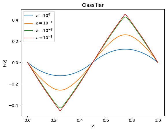
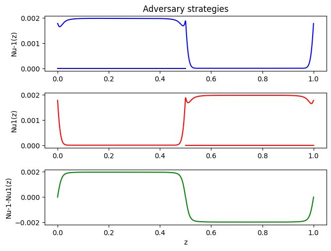
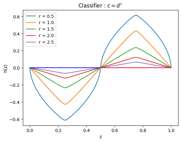
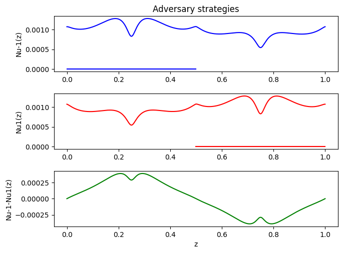
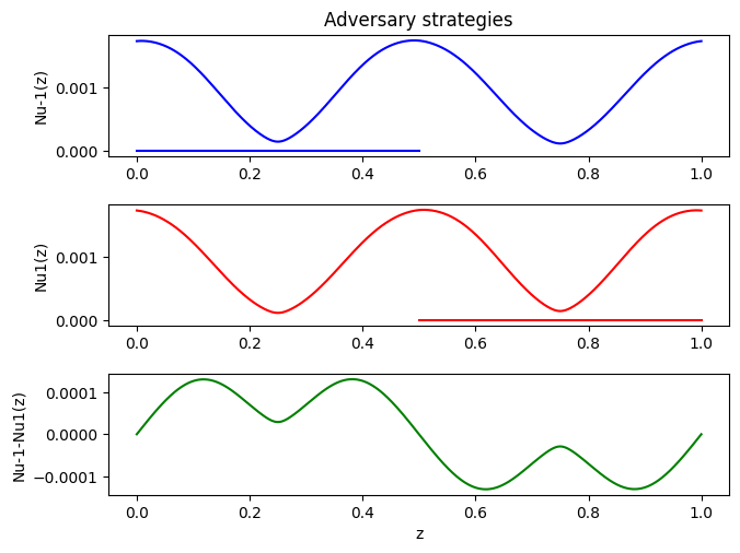
Impact of . In this paragraph, we look at the impact of . We set the measure supported on with uniform density with respect to and the measure supported over with uniform density with respect to . The cost is taken to be equal to the distance on the torus. In Figure 1(a), we show the classifier we obtain for different values of . As decreases the classifier becomes less and less regular and more and more confident. This is a direct consequence of the fact that the larger the the more the adversary will be able to move mass around. Note that the singularity of the optimal adversarial attack, which involves splitting the mass, only appears for .

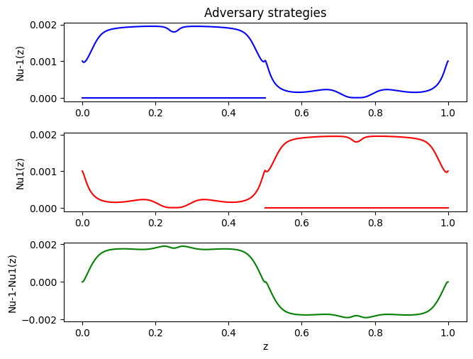
Impact of the cost. We now look at the impact of the power on the distance. The measures are the same as in the study of the impact of . The regularity parameter is taken to be equal to . In Figure 2(a), we display the classifer we obtain for different costs of the form for . Notice that as the power increases it becomes less and less costly for the adversary to move mass arround. This is coherent with the fact the absolute value of the classifier decreases with . Note as well that as increases and become closer and closer. It is also worth noting the cusp of the optimal attack for the square root cost.
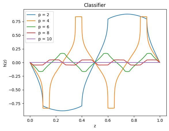
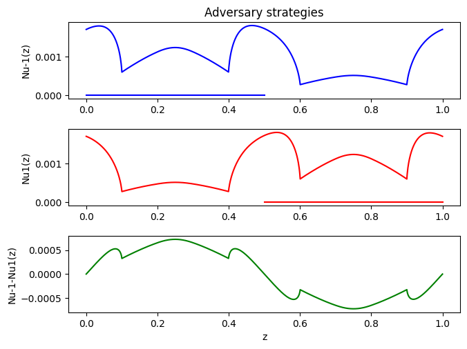
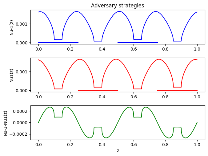
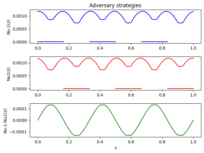
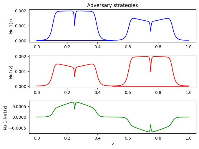
Impact of the initial measures. Finally, we take a discontinuous cost which prevents the adversary from moving mass too far away, namely . The measures are taken to be constant over interleaving intervals of growing number . More precisely, is uniform over and is uniform over the complement. Figure 3(a) shows the evolution of the classifiers with the total number of intervals. When there are intervals it is possible for the adversary to match and without incurring any cost. This explains that the classifier cannot distinguishs between the two measures.
6 Conclusions
In this work, we have considered a zero-sum game between a player designing a soft binary classifier and an adversary who may corrupt the true distributions at the expense of some transport cost. Under some mild regularity assumptions on the loss and transport cost functions, we have shown that this game has a value. More importantly, in our opinion, we established the existence of continuous optimal classifiers by exploiting some specific properties of a convex minimization problem (see (3.1)) sharing some similarities with the Kantorovich dual formulation of optimal transportation. We also proposed a softmax approximation of this problem, studied its convergence, as the regularization parameter vanishes, and presented some numerical simulations based on this approximation. In these simulations, we considered toy one-dimensional situations (not because of special properties of optimal transport in one dimension but because of the dimension of the softmax approximation which involves integrations with respect to a reference measure with full suport).
Among possible perspectives, let us mention, on the theoretical side, the extension of our analysis to adversarial multi-class classification [11]. On the computational side, investigating efficient schemes that are able to treat more realistic higher-dimensional examples would be desirable.
Acknowledgments: G.C. acknowledges the support of the Lagrange Mathematics and Computing Research Center.
References
- [1] Martin Arjovsky, Soumith Chintala, and Léon Bottou. Wasserstein generative adversarial networks. In Doina Precup and Yee Whye Teh, editors, Proceedings of the 34th International Conference on Machine Learning, volume 70 of Proceedings of Machine Learning Research, pages 214–223. PMLR, 06–11 Aug 2017.
- [2] Waïss Azizian, Franck Iutzeler, and Jérôme Malick. Regularization for Wasserstein distributionally robust optimization. ESAIM Control Optim. Calc. Var., 29:Paper No. 33, 31, 2023.
- [3] Dimitri P. Bertsekas and Steven E. Shreve. Stochastic optimal control, volume 139 of Mathematics in Science and Engineering. Academic Press, Inc. [Harcourt Brace Jovanovich, Publishers], New York-London, 1978. The discrete time case.
- [4] Jose Blanchet, Yang Kang, and Karthyek Murthy. Robust Wasserstein profile inference and applications to machine learning. J. Appl. Probab., 56(3):830–857, 2019.
- [5] Andrea Braides. -convergence for beginners, volume 22 of Oxford Lecture Series in Mathematics and its Applications. Oxford University Press, Oxford, 2002.
- [6] Marco Cuturi. Sinkhorn distances: Lightspeed computation of optimal transport. Advances in Neural Information Processing Systems, 26, 2013.
- [7] Marco Cuturi and Arnaud Doucet. Fast computation of wasserstein barycenters. In International conference on machine learning, pages 685–693. PMLR, 2014.
- [8] Simone Di Marino and Augusto Gerolin. An optimal transport approach for the Schrödinger bridge problem and convergence of Sinkhorn algorithm. J. Sci. Comput., 85(2):Paper No. 27, 28, 2020.
- [9] Ivar Ekeland and Roger Témam. Convex analysis and variational problems, volume 28 of Classics in Applied Mathematics. Society for Industrial and Applied Mathematics (SIAM), Philadelphia, PA, english edition, 1999. Translated from the French.
- [10] Nicolás García Trillos, Jakwang Kim, and Matt Jacobs. The multimarginal optimal transport formulation of adversarial multiclass classification. J. Mach. Learn. Res., 24:Paper No. [45], 56, 2023.
- [11] Nicolás García Trillos, Jakwang Kim, and Matt Jacobs. The multimarginal optimal transport formulation of adversarial multiclass classification. J. Mach. Learn. Res., 24:Paper No. [45], 56, 2023.
- [12] Ian Goodfellow, Jean Pouget-Abadie, Mehdi Mirza, Bing Xu, David Warde-Farley, Sherjil Ozair, Aaron Courville, and Yoshua Bengio. Generative adversarial nets. In Z. Ghahramani, M. Welling, C. Cortes, N. Lawrence, and K.Q. Weinberger, editors, Advances in Neural Information Processing Systems, volume 27. Curran Associates, Inc., 2014.
- [13] Ian J. Goodfellow, Jonathon Shlens, and Christian Szegedy. Explaining and harnessing adversarial examples. In Yoshua Bengio and Yann LeCun, editors, 3rd International Conference on Learning Representations, ICLR 2015, San Diego, CA, USA, May 7-9, 2015, Conference Track Proceedings, 2015.
- [14] Christian Léonard. From the Schrödinger problem to the Monge-Kantorovich problem. J. Funct. Anal., 262(4):1879–1920, 2012.
- [15] Aleksander Madry, Aleksandar Makelov, Ludwig Schmidt, Dimitris Tsipras, and Adrian Vladu. Towards deep learning models resistant to adversarial attacks. In International Conference on Learning Representations, 2018.
- [16] Laurent Meunier, Meyer Scetbon, Rafael B Pinot, Jamal Atif, and Yann Chevaleyre. Mixed nash equilibria in the adversarial examples game. In Marina Meila and Tong Zhang, editors, Proceedings of the 38th International Conference on Machine Learning, volume 139 of Proceedings of Machine Learning Research, pages 7677–7687. PMLR, 18–24 Jul 2021.
- [17] Peyman Mohajerin Esfahani and Daniel Kuhn. Data-driven distributionally robust optimization using the Wasserstein metric: performance guarantees and tractable reformulations. Math. Program., 171(1-2):115–166, 2018.
- [18] Marcel Nutz. Introduction to Entropic Optimal Transport, 2021.
- [19] Gabriel Peyré and Marco Cuturi. Computational optimal transport: With applications to data science. Foundations and Trends® in Machine Learning, 11(5-6):355–607, 2019.
- [20] Rafael Pinot, Raphael Ettedgui, Geovani Rizk, Yann Chevaleyre, and Jamal Atif. Randomization matters how to defend against strong adversarial attacks. In Hal Daumé III and Aarti Singh, editors, Proceedings of the 37th International Conference on Machine Learning, volume 119 of Proceedings of Machine Learning Research, pages 7717–7727. PMLR, 13–18 Jul 2020.
- [21] Walter Rudin. Real and complex analysis. McGraw-Hill Book Co., New York, third edition, 1987.
- [22] Filippo Santambrogio. Optimal transport for applied mathematicians, volume 87 of Progress in Nonlinear Differential Equations and their Applications. Birkhäuser/Springer, Cham, 2015. Calculus of variations, PDEs, and modeling.
- [23] Christian Szegedy, Wojciech Zaremba, Ilya Sutskever, Joan Bruna, Dumitru Erhan, Ian J. Goodfellow, and Rob Fergus. Intriguing properties of neural networks. In Yoshua Bengio and Yann LeCun, editors, 2nd International Conference on Learning Representations, ICLR 2014, Banff, AB, Canada, April 14-16, 2014, Conference Track Proceedings, 2014.
- [24] Nicolas Garcia Trillos, Matt Jacobs, and Jakwang Kim. On the existence of solutions to adversarial training in multiclass classification, 2023.
- [25] Nicolas Garcia Trillos, Matt Jacobs, Jakwang Kim, and Matthew Werenski. An optimal transport approach for computing adversarial training lower bounds in multiclass classification, 2024.
- [26] Cédric Villani. Topics in optimal transportation, volume 58 of Graduate Studies in Mathematics. American Mathematical Society, Providence, RI, 2003.