Bayesian Selection for Efficient MLIP Dataset Selection

Abstract

The problem of constructing a dataset for MLIP development which gives the maximum quality in the minimum amount of compute time is complex, and can be approached in a number of ways. We introduce a “Bayesian selection” approach for selecting from a candidate set of structures, and compare the effectiveness of this method against other common approaches in the task of constructing ideal datasets targeting Silicon surface energies. We show that the Bayesian selection method performs much better than Simple Random Sampling at this task (for example, the error on the (100) surface energy is 4.3x lower in the low data regime), and is competitive with a variety of existing selection methods, using ACE [1] and MACE [2] features.

• 1. Warwick Centre for Predictive Modelling, School of Engineering, University of Warwick, Coventry CV4 7AL, United Kingdom

• February 2025

1 Introduction

Efficient dataset construction forms an important part of generating Machine Learning Interatomic Potentials (MLIPs) for new materials. The greatest contributor to the computational cost of adding structures to a dataset is almost always the evaluation of DFT and other QM methods to obtain energy and force data, rather than in the generation of atomic positions alone.

Given a set of candidate structures, we can leverage sampling techniques to attempt to select a subset of structures which will maximally improve the quality of a MLIP model whilst requiring the least computational time possible. There are many different routes to this initial set of candidate structures, for example running Molecular Dynamics (MD) simulations with a potential, using random atom or cell displacements, random swaps of atoms, or generating structures using some continuum displacement law or experimentally known reconstruction. With the recent development of several “foundation model” [3, 4, 5, 6, 7, 8] potentials (models which attempt to describe all of materials chemistry), generating sets of candidate structures prior to performing DFT is increasingly accessible for more complex systems and properties.

Many approaches to the general problem of efficient dataset generation have already been proposed [9, 10, 11, 12, 13, 14, 15, 16]. Subramanyam and Perez [9] propose a scheme attempting to maximise the informational entropy of descriptor vectors contained in the dataset. Candidate structures are generated randomly, and the log determinant of the empirical covariance of descriptor vectors is used to define the informational entropy, assuming the descriptor vectors are independent and identically distributed (iid).

The ACE HyperActive Learning approach (HAL/ACEHAL) [10] by van der Oord et. al. uses a committee of Atomic Cluster Expansion (ACE) models, which are sampled from the Bayesian posterior on the ACE weights. They use this committee to specify a biasing potential derived from the committee variance, which then allows for acquisition of structures with large predicted error through biased Molecular Dynamics (MD) simulations. Structures are sampled from MD by means of a selection function with some initialised triggering tolerance. The main drawback of this approach is that it is a “one-shot” process - the full committee is be retrained based on the DFT results of the selected structure after each selection, which makes the scalability of such a solution limited.

To investigate the effectiveness of sampling techniques on this problem, we propose several methods which combine an atomistic descriptor with a standard sampling technique to provide a training dataset. Each method was applied to structures targeting surfaces in the 2018 Silicon GAP dataset [17] in order to generate a sub-dataset. Each sub-dataset was combined with bulk structures from the same original dataset to form a complete training dataset for an MLIP model.

Models trained on each of the datasets were then benchmarked based on the RMSE errors on energies and forces applied to all bulk and surface structures, as well as the predicted (100) and (111) surface energies.

2 Sampling Methodology

Although the Si dataset contains energy and force information for each structure (and a subset contain virial stresses), these properties are not used to inform sampling methods applied here. The aim of the work was to evaluate methods which only rely on atomic positions, such tha we could perform the selection prior to DFT calculations. Each sampling method uses a local, atom-centered descriptor to define a structure-level feature vector using the average of the atomic features.

ACE [1] is a fixed-form descriptor used to construct ACE linear models. We use three different parameterisations of the descriptor to test the tradeoff between increased information contained in the descriptor vector, and the corrseponding increase in dimensionality.

Table 1: Parameterisation of ACE descriptors, and lengths of all descriptor vectors

Descriptor	Order	Degree	Learnable	Length
ACE (S): “Small”	3	12	X	211
ACE (M): “Medium”	3	16	X	668
ACE (L): “Large”	3	19	X	1429
MACE (C): “Core”			✓	640
MACE (T): “Total”			✓	640
MP0 Foundation			✓	640

MACE [2] uses a learnable atomic embedding in a message passing network, with the representation initially based on the ACE descriptor to form the equivalent of a descriptor. The MP0 foundation model [3] was used as an initial baseline for the performance of MACE in the sparsification task, and two bespoke MACE models were trained on Si bulk (“Core” dataset), and Si bulk + surfaces (“Total” dataset) in order to evaluate whether training the embedding provides any benefit.

Table 2: Table showing the conversion from the full 2018 database into the “Core” Dataset, and the “Total” = Core + “Sampling” dataset. The Core dataset covers bulk, elasticity, and some low temperature bulk MD data. The Sampling dataset contains information about surfaces.

2018 Database	“Core”	“Total”		# Atoms
Config Type	Dataset	Dataset	# Structures	per Structure
isolated_atom	✓	✓	1	1
dia (Si Bulk)	✓	✓	104	2
			220	16
			110	54
			55	128
surface_001		✓	29	144
surface_110		✓	26	108
surface_111		✓	47	96
surface_111_pandey		✓	50	96
surface_111_3x3_das		✓	1	52
decohesion		✓	11	16
			11	24
			11	32
Total (“Core” Dataset)			490
Total (“Total” Dataset)			676

From the set of structure level features, common sparsification techniques were applied in order to provide sampling of the structures. The $k$-medoids [18] algorithm partitions the set of features into $k$ clusters (where in this case $k$ is the number of structures we wish to select), and returns the median coordinate of each cluster. Farthest Point Sampling (FPS) [19] requires some initial state, often by choosing a single feature vector randomly - in this case we initialise with the set of core dataset features. For each iteration, the method defines a distance metric between each candidate feature and the current state, and selects the candidate feature with the largest associated distance.

We also test an approach derived from the CUR method by Mahoney and Drineas [20]. They use a normalised statistical leverage score as a probability distribution, with which they can sample columns and rows of a matrix $A$ in order to produce an accurate CUR decomposition. We can use this scoring scheme to provide a probability distribution over features, and then sample from this distribution in order to select structures. We test two variants of this approach: the first is to use the structure level features similarly to the preceding approaches, and the second is to calculate scores on the atomic descriptor features directly, and sum scores for each feature in a structure.

2.1 HAL-style Bayesian selection

We can also define another sampling strategy using ideas from Bayesian linear regression [21], and the posterior covariance. Given a linear model in an atomic energy $E(x)=\Phi(x)\alpha$, with some design matrix $\Phi(x)_{ij}=\phi_{j}(x_{i})$ formed of basis functions $\{\phi_{j}(x)\}$ of the atomic descriptor $x$, and model weights $\alpha$, we can analytically compute the Bayesian posterior distribution $\alpha\sim\mathcal{N}(\mu,\Sigma)$, where:

$$\Sigma^{-1}=\Phi^{T}\Lambda\Phi+\Sigma_{0}^{-1}$$ (1)

$$\mu=\Sigma\Phi^{T}\Lambda^{\frac{1}{2}}y$$ (2)

From this, it is apparent that the posterior covariance $\Sigma$ does not depend on the observations $y$ - only the design matrix $\Phi$, prior covariance matrix $\Sigma_{0}$, and likelihood precision matrix $\Lambda$ are required (the prior covariance and likelihood precision can be expressed as hyperparameters of the Bayesian model).

For some new candidate observation $(x^{*},y^{*})$, we can define score functions based on the design matrix $\Phi^{*}$ associated with this new observation. Evaluating this score function on a set of candidate structures, we select the structure with the highest associated score, and update the posterior covariance

$$\Sigma_{n+1}^{-1}=\begin{pmatrix}\Phi_{n}\\ \Phi^{*}\end{pmatrix}^{T}\begin{pmatrix}\Lambda_{n}&0\\ 0&\Lambda^{*}\end{pmatrix}\begin{pmatrix}\Phi_{n}\\ \Phi^{*}\end{pmatrix}+\Sigma_{0}^{-1}\equiv\Phi^{*T}\Lambda^{*}\Phi^{*}+\Sigma_{n}^{-1}$$ (3)

Here, $\Sigma_{n}$ is the posterior covariance matrix of the $n^{\text{th}}$ iteration, trained with design matrix $\Phi_{n}$, and $\Phi^{*}$ is the design vector of the newly selected point $x^{*}$

The choice of which score function to use in selecting each structure leads to differing results. The entropy of a set of random variables distributed as a multivariate normal is proportional to the log determinant of the covariance matrix, so by choosing the score function to be

$$\begin{split}H_{n}(\Phi^{*}_{k})&=\log|\Sigma_{k}^{*}|\\ &\equiv\log\left|\left[\begin{pmatrix}\Phi_{n}\\ \Phi^{*}_{k}\end{pmatrix}^{T}\begin{pmatrix}\Lambda_{n}&0\\ 0&\Lambda^{*}_{k}\end{pmatrix}\begin{pmatrix}\Phi_{n}\\ \Phi^{*}_{k}\end{pmatrix}+\Sigma_{0}^{-1}\right]^{-1}\right|\\ &=-\log\left|\Sigma_{n}^{-1}+\Phi^{*T}_{k}\Lambda^{*}_{k}\Phi^{*}_{k}\right|\end{split}$$ (4)

we can transform the approach into a variant of the previous work by Subramanyam and Perez.

We an also use the posterior in a manner similar to HAL, by defining the score function based on the posterior predictive uncertainty of observables. Some simple examples include the variance in per-atom energy

$$\mathrm{Var}(E_{\text{per-atom}})=\frac{1}{N^{2}}\sum_{ij}\left(\Phi_{E}^{*}\Sigma\Phi_{E}^{*T}\right)_{ij}$$ (5)

or the maximum force variance

$$\max_{i}(\mathrm{Var}(F_{i}))=\max_{i}\left[\left(\Phi_{F}^{*}\Sigma\Phi_{F}^{*T}\right)_{ii}\right]$$ (6)

We can use this approach to generalise the ACEHAL approach: given any general MLIP model $E_{\text{MLIP}}(x)=f_{\text{MLIP}}(x,\alpha_{\text{MLIP}})$ ($f_{\text{MLIP}}$ could be nonlinear in the weights), we can define a linear surrogate in terms of the atomic descriptor $x$, with posterior covariance

$$\begin{split}&\Sigma^{-1}=\Phi^{T}\Lambda\Phi+\Sigma_{0}^{-1}\end{split}$$ (7)

where $\Phi_{ij}=\{x_{j}\}_{i}$ is a design matrix formed of the atomic descriptor evaluations.

We could then perform biased MD simulations exactly as HAL does: using the true MLIP model to describe the true potential energy surface, and using the linear surrogate to inform the uncertainty-based biasing potential. We can also update the posterior covariance (using Eqn. 3) of the surrogate with each structure selected.

One key advantage of this procedure is the relaxation of the HAL “one-shot” scheme to an “$N$-shot” scheme (where $N$ is the number of structures added to the dataset before the MLIP model is retrained), increasing the throughput of the process by deferring DFT and refits to occur in batches, instead of after every selection.

With standard HAL, if we had instead selected $N$ structures without refitting the committee, we would not account for correlations in the structures selected. We therefore may oversample regions of previously high uncertainty, which may have only required a single structure to correct. The Bayesian selection approach fixes this oversampling issue by providing an update to the posterior covariance (which is what defines the variance of the committee and thus the sampling metric) after each of the structure is drawn.

Since we build a linear surrogate to form the biasing potential, we are not restricted to descriptor features from linear models - we are also able to leverage learnable descriptor features such as the features of the MACE descriptor.

3 Results

Figures 1 and 2 compare the performance of using the ACE descriptor as an input to each of the sampling methods, at a range of different dataset sizes (each dataset is the full “Core” dataset, plus a small number of surface structures sampled from a larger pool of available data).

Figure 1 makes this comparison in terms of the RMSE error on energies and forces across all of the “Core” bulk structures, and the full pool of surface structures. The sampling methods have nearly equivalent force errors, but Bayesian selection is approximately 5 meV/Å worse across the dataset for $N=20$, where $N$ is the number of surface structures included in training, and $k$-medoids being around 30 meV/Å worse at $N=10$ (both methods get much closer to average when the dataset size is increased). The energy errors show a different picture, with $k$-medoids and Bayesian selection being better for $N\geq 5$ (k-medoids is around 2.5 meV/atom better than SRS at $N=20$). Both CUR-based methods perform comparably with SRS across all dataset sizes, and FPS sampling performs consistently poorly in terms of energy errors when compared to SRS ($\approx$4.8 mev/atom worse at $N=20$; similar difference at $N=100$).

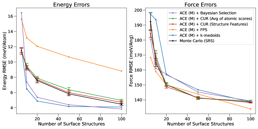
Figure 1: A comparison of the energy (left) and force (right) RMSE errors across the “Total” dataset, using the “Medium” parameterisation of the ACE descriptor as an input space for various standard sparsification methods.

Figure 2 compares the error on predicted (100) and (111) surface energies when compared to DFT, for the same set of sampling methods using the ACE descriptor. Here, $k$-medoids and Bayesian selection do very well at predicting the (100) surface energy, consistently giving results to an error of under 0.05 J/m² for all $N$. The methods are also the best performing for the (111) surface energy, with $k$-medoids incurring less error for $N>10$, but having significantly higher error for $N=5$. Again CUR performs comparably to SRS, with predictions of the (100) surface being on average worse. Using CUR with structure features appears to work slightly better than SRS on the (111) surface, but the two results are extremely close. FPS consistently performs the worst on the (111) surface, with an error at $N=100$ that is around 0.18 J/m² higher than CUR with score averaging, which is the next worst performing method here. FPS is also poor at predicting an accurate (100) surface energy for $N<50$, after which it constructs datasets of similar quality to the CUR approaches.

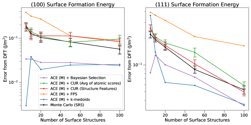
Figure 2: A comparison of the error on predictions of the (100) (left) and (111) (right) surface energies, using the “Medium” parameterisation of the ACE descriptor as an input space for various standard sparsification methods.

To compare the relative performance of each descriptor, we limit the methods to $k$-medoids and Bayesian selection as these appear to be the best performing methods in the “Medium” ACE descriptor. Figure 3(a) shows the overall energy and force RMSE errors for each of the choices of descriptor applied to the $k$-medoids method. We see that all of the descriptors perform better than SRS in terms of energy RMSE, and near equivalent in terms of force RMSE. Most descriptors perform very similarly, but the “Total” MACE descriptor appears to be the worst performing at predicting energies, but the best at predicting forces.

Figure 3(b) shows the equivalent comparison for the Bayesian selection method. We see a similar picture for the force error, where the descriptors are approximately equal with SRS, but we see a different picture for energy errors. At $N=5$ we see that the “Medium” and “Large” ACE descriptors perform considerably worse than SRS, but that they become significantly better for $N=10$, where the “Large” descriptor has 4 meV/Atom lower energy RMSE than SRS.

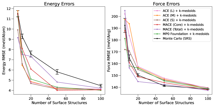
(a) Dataset RMSE Errors, using $k$-medoids sampling on different descriptors

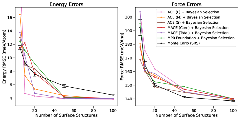
(b) Dataset RMSE Errors, using Bayesian selection on different descriptors

Figure 3: Comparison of the energy and force RMSE errors over the “Total” dataset. Each subplot shows a range of common descriptor functions used to provide an input to each of the standard sparsification methods.

Figure 4(a) compares the descriptors across surface energy predictions. We see that initially the MP0, “Core” MACE, and “Large” ACE descriptors perform worse than SRS at predicting the (100) energy for $N=5$, but that all descriptors become much better than SRS for $N>5$. The “Total” MACE descriptor is the worst performing at predcting the (100) energy for $10\leq N\leq 50$. For the (111) surface, we see that MP0, “Core” MACE, and the “Small” and “Medium” ACE descriptors perform worse than SRS initially, but almost al of the descriptors become much better than SRS for $N>10$. The exception is the “Total” MACE descriptor, which performs equivalently to SRS for $N\geq 20$.

Figure 4(b) shows the surface energy comparison for the Bayesian selection method. Here, we see that all descriptors perform extremely well at predicting the (100) surface, even for small $N$, and the choice of descriptor does not appear to significantly affect the error. On the (111) surface, we see that all descriptors using BLR perform better than SRS for $N\geq 20$, with the “Medium” and “Large” ACE descriptors consistently performing better for all $N$. The “Core” and “Total” MACE descriptors also perform competitively for $N\geq 20$, but perform worse than SRS at $N=5$.

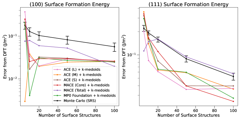
(a) Error on surface energy predictions, using $k$-medoids sampling on different descriptors

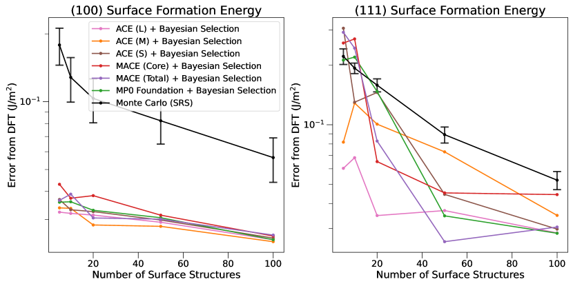
(b) Error on surface energy predictions, using Bayesian selection on different descriptors

Figure 4: Errors on (100) and (111) surface energies (compared with DFT). Each panel shows a range of common descriptor functions used to provide an input to each of the sparsification methods.

4 Discussion

It is clear from Figs. 1 & 2 that the choice of sparsification method does impact the performance of resulting MLIP models, both in terms of training RMSE errors, and in predictions of key quantities. It is ultimately difficult to argue that any one method is universally the “best”, due to the work focussing on a single test case, but our results support the use of $k$-medoids and Bayesian selection. The results also show that these methods were consistently competitive against SRS across a range of different descriptors.

Although $k$-medoids and Bayesian selection perform comparably on the chosen tests, Bayesian selection may be a better choice for expanding on existing datasets, as we are able to use the posterior formed from the existing dataset as the new prior for the selection process. We could also improve the method by attempting to encode more information into the sparsification process: by including force and/or stress contributions to the Bayesian posterior, and also by customising the scoring function based on desired outcomes (i.e. by using a scoring metric based on forces to target improvements to force predictions, or by using a weighted sum of several metrics).

We also see that the Bayesian selection method generates models which are significantly closer to DFT for the (100) surface energy, when compared to the (111) surface energy. This is likely due to the many physical (111) surface reconstructions, of which three are included in the dataset, and only one is tested.

5 Conclusions

A new Bayesian selection method, derived from Bayesian linear regression, was developed for the purpose of sampling structures from a candidate set, with the aim of producing a concise dataset which maximally improves MLIP model accuracy. We show that the method is effective at producing “good” datasets, where models trained on these datasets accurately reproduce targeted quantities of interest, for the given test case. We also show that the method performs better than some competing approaches at the given task, and that it remains similarly effective for a number of atomic descriptors.

6 Data Availability

Data and scripts required to reproduce this work are provided by a GitHub repository, and corresponding Zenodo archive [22].

7 Acknowledgments

T.R is supported by a studentship within the Engineering and Physical Sciences Research Council supported Centre for Doctoral Training in Modelling of Heterogeneous Systems, Grant No. EP/S022848/1, with additional funding from Huawei Technologies R&D UK.

We acknowledge usage of the ARCHER2 facility for which access was obtained via the UKCP consortium and funded by EPSRC Grants No. EP/P022561/1 and No. EP/X035891/1. Calculations were performed using the Sulis Tier 2 HPC platform hosted by the Scientific Computing Research Technology Platform at the University of Warwick. Sulis is funded by EPSRC Grant EP/T022108/1 and the HPC Midlands+ consortium. Further computing facilities were provided by the Scientific Computing Research Technology Platform of the University of Warwick.

8 References

References

- [1] Ralf Drautz “Atomic cluster expansion for accurate and transferable interatomic potentials” In Phys. Rev. B 99 American Physical Society, 2019, pp. 014104 DOI: 10.1103/PhysRevB.99.014104
- [2] Ilyes Batatia et al. “MACE: Higher Order Equivariant Message Passing Neural Networks for Fast and Accurate Force Fields”, 2023 arXiv: https://arxiv.org/abs/2206.07697
- [3] Ilyes Batatia et al. “A foundation model for atomistic materials chemistry”, 2024 arXiv: https://arxiv.org/abs/2401.00096
- [4] Luis Barroso-Luque et al. “Open Materials 2024 (OMat24) Inorganic Materials Dataset and Models”, 2024 arXiv: https://arxiv.org/abs/2410.12771
- [5] Mark Neumann et al. “Orb: A Fast, Scalable Neural Network Potential”, 2024 arXiv: https://arxiv.org/abs/2410.22570
- [6] Han Yang et al. “MatterSim: A Deep Learning Atomistic Model Across Elements, Temperatures and Pressures”, 2024 arXiv: https://arxiv.org/abs/2405.04967
- [7] Amil Merchant et al. “Scaling deep learning for materials discovery” In Nature 624.7990, 2023, pp. 80–85 DOI: 10.1038/s41586-023-06735-9
- [8] Anton Bochkarev, Yury Lysogorskiy and Ralf Drautz “Graph Atomic Cluster Expansion for Semilocal Interactions beyond Equivariant Message Passing” In Phys. Rev. X 14 American Physical Society, 2024, pp. 021036 DOI: 10.1103/PhysRevX.14.021036
- [9] Aparna P.. Subramanyam and Danny Perez “Information-entropy-driven generation of material-agnostic datasets for machine-learning interatomic potentials”, 2024 arXiv: https://arxiv.org/abs/2407.10361
- [10] Cas van der Oord et al. “Hyperactive Learning (HAL) for Data-Driven Interatomic Potentials”, 2022 arXiv: https://arxiv.org/abs/2210.04225
- [11] Evgeny V. Podryabinkin, Evgeny V. Tikhonov, Alexander V. Shapeev and Artem R. Oganov “Accelerating crystal structure prediction by machine-learning interatomic potentials with active learning” In Phys. Rev. B 99 American Physical Society, 2019, pp. 064114 DOI: 10.1103/PhysRevB.99.064114
- [12] Ivan S Novikov, Konstantin Gubaev, Evgeny V Podryabinkin and Alexander V Shapeev “The MLIP package: moment tensor potentials with MPI and active learning” In Machine Learning: Science and Technology 2.2 IOP Publishing, 2020, pp. 025002 DOI: 10.1088/2632-2153/abc9fe
- [13] Lars L. Schaaf et al. “Accurate energy barriers for catalytic reaction pathways: an automatic training protocol for machine learning force fields” In npj Computational Materials 9.1, 2023, pp. 180 DOI: 10.1038/s41524-023-01124-2
- [14] Ji Qi et al. “Robust training of machine learning interatomic potentials with dimensionality reduction and stratified sampling” In npj Computational Materials 10.1, 2024, pp. 43 DOI: 10.1038/s41524-024-01227-4
- [15] M Hodapp and A Shapeev “In operando active learning of interatomic interaction during large-scale simulations” In Machine Learning: Science and Technology 1.4 IOP Publishing, 2020, pp. 045005 DOI: 10.1088/2632-2153/aba373
- [16] Christoph Dösinger et al. “Efficient descriptors and active learning for grain boundary segregation” In Phys. Rev. Mater. 7 American Physical Society, 2023, pp. 113606 DOI: 10.1103/PhysRevMaterials.7.113606
- [17] Albert P. Bartók, James Kermode, Noam Bernstein and Gábor Csányi “Machine Learning a General-Purpose Interatomic Potential for Silicon” In Phys. Rev. X 8 American Physical Society, 2018, pp. 041048 DOI: 10.1103/PhysRevX.8.041048
- [18] Leonard Kaufman and Peter J. Rousseeuw “Partitioning Around Medoids (Program PAM)” In Finding Groups in Data John Wiley & Sons, Ltd, 1990, pp. 68–125 DOI: https://doi.org/10.1002/9780470316801.ch2
- [19] Yuval Eldar, Michael Lindenbaum, Moshe Porat and Yehoshua Zeevi “The Farthest Point Strategy for Progressive Image Sampling” In IEEE transactions on image processing : a publication of the IEEE Signal Processing Society 6, 1997, pp. 1305–15 DOI: 10.1109/83.623193
- [20] Michael W. Mahoney and Petros Drineas “CUR matrix decompositions for improved data analysis” In Proceedings of the National Academy of Sciences 106.3, 2009, pp. 697–702 DOI: 10.1073/pnas.0803205106
- [21] Christopher M. Bishop and Michael E. Tipping “Bayesian Regression and Classification” In Advances in Learning Theory: Methods, Models and Applications, NATO Science Series, III: Computer and Systems Sciences United States: IOS Press, 2003, pp. 267–285
- [22] Thomas Rocke and James Kermode “Bayesian Selection code for MLIP Dataset Selection” Zenodo, 2025 DOI: 10.5281/zenodo.14945864