BBGKY hierarchy for quantum error mitigation

Abstract

Mitigation of quantum errors is critical for current NISQ devices. In the current work, we address this task by treating the execution of quantum algorithms as the time evolution of an idealized physical system. We use knowledge of its physics to assist the mitigation of the quantum noise produced on the real device. In particular, the time evolution of the idealized system obeys a corresponding BBGKY hierarchy of equations. This is the basis for the novel error mitigation scheme that we propose. Specifically, we employ a subset of the BBGKY hierarchy as supplementary constraints in the ZNE method for error mitigation. We ensure that the computational cost of the scheme scales polynomially with the system size. We test our method on digital quantum simulations of the lattice Schwinger model under noise levels mimicking realistic quantum hardware. We demonstrate that our scheme systematically improves the error mitigation for the measurements of the particle number and the charge within this system. Relative to ZNE we obtain an average reduction of the error by 18.2% and 52.8% for the respective above observables. We propose further applications of the BBGKY hierarchy for quantum error mitigation.

I Introduction

The coupling of quantum computers to their surrounding environment is unavoidable, hence efficient methods to reduce quantum noise are highly demanded. While the general theory of quantum error correction offers a framework to achieve fully fault-tolerant computations [1, 2, 3, 4], its required qubit overhead remains prohibitively high for today’s quantum devices [5]. As an alternative to the currently challenging quantum error correction, quantum error mitigation (QEM) approaches were proposed [6, 7, 8, 9, 10, 11, 12, 13, 14]. Despite their fundamental limitations [15, 16], they remain the main available tools for the current noisy intermediate-scale quantum (NISQ) devices [17] and for the upcoming early phases of fault-tolerant computing [18, 19, 20].

In this work, we empirically investigate how additional information provided by physics can improve the performance of QEM. The cornerstone idea of our approach is that the time-evolved state of any noiseless quantum system, at any time during the computation process, obeys a corresponding Schrödinger equation, so physical laws can be used to verify quantum computations. Unfortunately, this idea alone is of small practical use, since a full quantum state tomography of exponentially many measurements is required for the perfect knowledge of the state. To employ this concept in practice, one has to dramatically reduce the number of necessary measurements, for instance by symmetry verification [21] or by using N-representability conditions [22].

In this paper, we employ the fact that the full dynamics of the idealized system of $N_{\text{Q}}$ qubits can be obtained from a quantum Bogoliubov-Born-Green-Kirkwood-Yvon (BBGKY) hierarchy [23, 24, 25, 26] of $4^{N_{\text{Q}}}$ equations. In classical computations, to avoid implementing an exponentially large system of coupled dynamical equations, one generally truncates the hierarchy by modeling the high-order correlators or by assuming their vanishing [27, 28, 29]. However, for strongly correlated systems or any general computational task, there are no (known) naturally small parameters justifying these truncations [30, 29]. In quantum computations, truncations are no longer necessary, as one can directly measure any observable from the quantum device. One can then use corresponding equations from the BBGKY hierarchy to test the correctness of the measurements, hence of the quantum computations.

In this paper, we use the important fact that the amount of terms in all hierarchical equations is bounded by $\text{poly}(N_{\text{Q}})$, and by focusing on $\text{poly}(N_{\text{Q}})$-large subsets of the hierarchy, only a polynomial in $N_{\text{Q}}$ amount of additional classical resources is needed for the above-mentioned tests. We employ these supplementary informations from the BBGKY hierarchy to improve the ZNE method [9, 31] in digital quantum simulations. Specifically, we formulate a novel QEM scheme and apply it to the Schwinger model [32] brought to quantum lattice simulations as a $\frac{1}{2}$-spin model in the particular implementation of [33]. The Schwinger model has been widely studied and used as a benchmark toy model for quantum computations, for instance in the recent works [34, 35, 33, 36, 37, 38, 39, 40].

The paper is structured as follows. In section II we derive and describe the BBGKY hierarchy. Section III is dedicated to our QEM method: in subsection III.1 we briefly review the ZNE scheme, in subsection III.2 we describe how we select the BBGKY equations from the hierarchy, and in subsection III.3 we present our QEM technique. In section IV we apply our method to the lattice Schwinger model. Finally in section V we conclude and discuss further potential applications of the method.

II The BBGKY hierarchy

We begin by deriving the BBGKY hierarchy and by discussing its properties.

Consider a quantum $\frac{1}{2}$-spin model composed of $N_{\text{Q}}$ qubits, each of which is labeled by an index $i\in\quantity{1,\dots,N_{\text{Q}}}=:S$. Let $A\subseteq S$ represent a subsystem of the spin model, and let

$$\sigma(A,(\mu_{i})_{i\in A}):=\prod_{i\in A}\sigma_{i}^{\mu_{i}}$$ (1)

define a Pauli string, where $\mu_{i}\in\quantity{1,2,3}$ and $\sigma_{i}^{\mu_{i}}$ is the Pauli operator acting on the $i$-th qubit in the $\mu_{i}$-th direction. Assume the model has an Hamiltonian of the form

$$H:=\frac{1}{2}\sum_{i\in S}h_{i}^{\mu}\sigma_{i}^{\mu}+\frac{1}{4}\sum_{\begin{subarray}{c}i,j\in S\\ i<j\end{subarray}}V_{ij}^{\mu\nu}\sigma_{i}^{\mu}\sigma_{j}^{\nu},$$ (2)

where $h_{i}^{\mu}$ is the interaction term of the $i$-th spin in the $\mu$-th direction with an external magnetic field, $V_{ij}^{\mu\nu}$ is the interaction potential term among the $i$-th and $j$-th spins of respective $\mu$-th and $\nu$-th directions, and where from now on Einstein’s summation is implied. Moreover, here and throughout the work, we set $\hbar=c=1$.

If one injects (1) and (2) into Ehrenfest’s theorem and computes all the commutators, one obtains [41]

$$\begin{split}\derivative{t}\expectationvalue{\prod_{i\in A}\sigma_{i}^{\mu_{i}}}&=\sum_{\begin{subarray}{c}i,j\in A\\ i\neq j\end{subarray}}\frac{V_{ij}^{\mu_{i}\nu}}{2}\varepsilon_{\mu_{j}\nu\lambda}\expectationvalue{\sigma_{j}^{\lambda}\prod_{k\in A\setminus\quantity{i,j}}\sigma_{k}^{\mu_{k}}}\\ &+\,\sum_{i\in A}h_{i}^{\lambda}\varepsilon_{\mu_{i}\lambda\nu}\expectationvalue{\sigma_{i}^{\nu}\prod_{j\in A\setminus\quantity{i}}\sigma_{j}^{\mu_{j}}}\\ &+\,\sum_{\begin{subarray}{c}i\in A\\ j\notin A\end{subarray}}\frac{V_{ij}^{\mu\nu}}{2}\varepsilon_{\mu_{i}\mu\lambda}\expectationvalue{\sigma_{i}^{\lambda}\sigma_{j}^{\nu}\prod_{k\in A\setminus\quantity{i}}\sigma_{k}^{\mu_{k}}},\end{split}$$ (3)

where $\varepsilon_{\mu\nu\lambda}$ is the three-dimensional Levi-Civita symbol. We call (3) the BBGKY equation of the $\sigma(A,(\mu_{i})_{i\in A})$ Pauli string. This is because, if one considers all the Pauli strings of all possible directions (namely all partitions $A\subseteq S$ of all possible $(\mu_{i})_{i\in A}$) then, by computing all their associated BBGKY equations (3), the complete exponentially large BBGKY-like hierarchy is generated. More precisely, for a specific Pauli string of length $\absolutevalue{A}=n\leq N_{\text{Q}}$, the time derivative of that $n$-point correlator is determined by a linear combination of $(n-1)$-point, $n$-point and $(n+1)$-point correlators, respectively found in the first, second and third summations of (3), all selected according to the values $h_{i}^{\mu}$ and $V_{ij}^{\mu\nu}$ in (2). The right-hand side (RHS) of (3) contains up to $9n(n-1)$-many $(n-1)$-point correlators, up to $9n$-many $n$-point correlators, and up to $27n(N_{\text{Q}}-n)$-many $(n+1)$-point correlators. Importantly, this implies that the amount of correlators in the RHS of (3) is polynomial in $n$ and $N_{\text{Q}}$, and bounded by $81N_{\text{Q}}^{2}/8$.

III Mitigation technique

In this section, we provide a short review of ZNE in the context of time evolution. Then we present our method, a BBGKY-improved ZNE scheme, which we formulate as a post-processing linear least-squares (LLSQ) optimization procedure. Our method incorporates a $\text{poly}(N_{\text{Q}})$-large subset of the BBGKY hierarchy evaluated across all time points. We consider the list of $l$ Pauli strings $\quantity{Q_{q}}_{q\in\quantity{0,\dots,l-1}}$, where for brevity $Q_{q}$ is defined as in (1). Our goal is to mitigate the corresponding measurements obtained from a realistic quantum device. We focus solely on Pauli strings because they form an operator basis for the observables of the system.

III.1 The ZNE method

By Trotterization, the evolution time $T$ is discretized into $N$ slices of duration $\Delta t:=T/N$, and evolution steps are obtained thanks to a Suzuki-Trotter decomposition scheme of order $d_{\text{ST}}$ [42, 43, 44, 45]. Then, different realizations of the quantum circuit implementing the time evolution are generated, each of them containing local unitary foldings [10] with a frequency of $\eta\geq 0$ insertions per step. Under the assumption that unitary foldings are affected by the same kind of noise as regular evolution steps, this implies an error level at the $s$-th step $s\in\quantity{0,\dots,N}$ relative to the original $\eta=0$ circuit of

$$1\leq\varepsilon_{s\eta}:=\frac{s+2\left\lfloor\eta s\right\rfloor}{s}\xrightarrow{s\to\infty}2\eta+1.$$ (4)

Performing the above $m$ times with different noise levels $\eta\in(\eta_{1},\dots,\eta_{m})=:\overrightarrow{\mathbf{\eta}}$, at each time point $t_{s}:=s\Delta t$, we end up with an experimentally measured set of data points $(\varepsilon_{s\eta},\expectationvalue{Q_{q}}_{s\eta})$, where $\expectationvalue{Q_{q}}_{s\eta}$ is the measurement of $Q_{q}$ at time point $t_{s}$, estimated with $N_{\text{S}}$ shots, under the $\eta$ noise level . For a given quantity at a given time point, these experimentally measured points can be interpolated across the error levels with a least-squares polynomial (LSP) in $\varepsilon$ of degree $d\leq m-1$, leading to a zero noise $\varepsilon\to 0$ extrapolated $\expectationvalue{Q^{0}_{q}}_{s}$ [10, 9].

III.2 Selection of BBGKY equations

Figure 1: In this diagram, $b$ is a Pauli string of interest, and $a_{1},c_{1}$ are $(n+1)$-point correlators, $a_{2},b,c_{2}$ are $n$-point correlators, and $a_{3},c_{3}$ are $(n-1)$-point correlators. All $c_{1},c_{2},c_{3}$ are downstream connected to $b$, and all $a_{1},a_{2},a_{3}$ are upstream connected to $b$.

Given the set of expectation values $\quantity{\expectationvalue{Q_{q}}}_{q\in\quantity{0,\dots,l-1}}$, the physical knowledge provided by a BBGKY equation can help their mitigation if and only if its associated Pauli string is hierarchically connected to any of the $\quantity{Q_{q}}_{q\in\quantity{0,\dots,l-1}}$.

For a given generic $\sigma(A,(\mu_{i})_{i\in A})$, the RHS of equation (3) provides all of the correlators $\sigma(B,(\nu_{i})_{i\in B})$, with $B\subseteq S$ of directions $(\nu_{i})_{i\in B}$, that are connected to its time evolution via the hierarchy. In that case, we say that the $\sigma(B,(\nu_{i})_{i\in B})$ are downstream connected to $\sigma(A,(\mu_{i})_{i\in A})$. We now want to determine the inverse, that is, given a Pauli string $\sigma(B,(\nu_{i})_{i\in B})$, find all correlators $\sigma(A,(\mu_{i})_{i\in A})$ generating $\sigma(B,(\nu_{i})_{i\in B})$ in their RHS of (3). In that case, we say that $\sigma(A,(\mu_{i})_{i\in A})$ is upstream connected to $\sigma(B,(\nu_{i})_{i\in B})$. Overall, we say that a correlator is connected to a Pauli string of interest if it is either downstream or upstream connected to that Pauli string.

To find all upstream connected correlators $\sigma(A,(\mu_{i})_{i\in A})$ to a given $\sigma(B,(\nu_{i})_{i\in B})$, there are only 3 possibilities: denoting $n_{A}=\absolutevalue{A}$ and $n_{B}=\absolutevalue{B}$, $\sigma(B,(\nu_{i})_{i\in B})$ can appear in the BBGKY equation of $\sigma(A,(\mu_{i})_{i\in A})$ either as an $(n_{A}+1)$-point, $n_{A}$-point or $(n_{A}-1)$-point correlator. The selection rules to find $\sigma(A,(\mu_{i})_{i\in A})$ candidates in all three cases are derived in appendix A. There we also show that, importantly, the upper bound for the amount of ansätze one has to check to pick up all the upstream connected $\sigma(A,(\mu_{i})_{i\in A})$ is polynomial in $N_{\text{Q}}$. Figure 1 schematically summarizes the two possible kinds of connections.

For our mitigation purposes, we select the BBGKY equations associated to the subset of the BBGKY hierarchy whose Pauli strings are connected to any of the $\quantity{Q_{q}}_{q\in\quantity{0,\dots,l-1}}$ by at most $r$ connections. The subset is obtained by iteratively computing over itself all of its downstream and upstream connected Pauli strings, as explained in appendix A, for a total of $r$ iterations. This generates a list of $g$ BBGKY equations containing $\Lambda\geq l$ correlators, the actual amount of expectation values $\quantity{\expectationvalue{Q_{q}}}_{q\in\quantity{0,\dots,l-1,l,\dots,\Lambda-1}}$ that have to be measured.

III.3 Our BBGKY-improved ZNE method

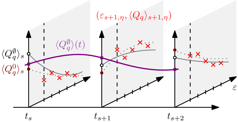
Figure 2: Schematic depiction of our method: each slice of data (red crosses) is interpolated with a LSP (dotted gray lines), producing a series of intermediate ZNEs (dark red points), which in turn are fitted with a Bernstein polynomial (purple line), giving access to time derivatives at each time point (purple squares). These are then used to improve the ZNEs thanks to the BBGKY equations, producing different LSPs (continuous gray lines) leading to BBGKY-improved ZNEs (black circles). The dashed black lines represent the $\varepsilon\geq 1$ bound.

Our method aims at improving the ZNE-obtained measurements $\expectationvalue{Q^{0}_{q}}_{s}$ with better BBGKY-constrained $\expectationvalue{Q^{\emptyset}_{q}}_{s}$ extrapolations. Because ZNE is a LLSQ minimization procedure, we want to incorporate the selected BBGKY equations as linear combinations of $\expectationvalue{Q^{\emptyset}_{q}}_{s}$. To do so, we approximate the time derivatives in (3) with derivatives of a Bernstein polynomial, fitting the $N+1$ extrapolated expectation values. We use (derivatives of) Bernstein polynomials because they are linear in the $\expectationvalue{Q^{\emptyset}_{q}}_{s}$ and because they uniformly converge to the functions (derivatives) they are fitting, with an error of the order $\order{1/N}$ [47]. Starting from the Bernstein polynomial [48]

$$\textstyle\expectationvalue{Q^{\emptyset}_{q}}(t):=\displaystyle\sum_{s=0}^{N}\textstyle\expectationvalue{Q^{\emptyset}_{q}}_{s}\displaystyle b_{sN}\quantity(\frac{t}{T}),$$ (5)

constructed out of the $N+1$ Bernstein polynomial basis elements $b_{sN}(x)$ of degree $N$, with $x\in\quantity[0,1]$ hence $t\in[0,T]$, then

$$\derivative{t}\textstyle\expectationvalue{Q^{\emptyset}_{q}}\displaystyle(t)=\sum_{s=0}^{N}\textstyle\expectationvalue{Q^{\emptyset}_{q}}_{s}\displaystyle\beta_{sN}\quantity(\frac{t}{T}),$$ (6)

where we define

$$\beta_{sN}(x):=\frac{1}{\Delta t}\begin{cases}-(1-x)^{N-1}&\text{if $s=0$}\\ x^{N-1}&\text{if $s=N$}\\ b_{s-1,N-1}(x)-b_{s,N-1}(x)&\text{otherwise}\\ \end{cases}.$$ (7)

Using the approximate time derivatives (6), approximations of the BBGKY equations (3) can be expressed as linear combinations of $\expectationvalue{Q^{\emptyset}_{q}}_{s}$. Thereby, BBGKY equations can be cast inside the original ZNE LLSQ procedure as additional constraints of the minimization problem

$$\operatorname*{argmin}_{\overrightarrow{\mathbf{a}}}\frac{1}{2}\norm{\overrightarrow{\mathbf{v}}(\overrightarrow{\mathbf{a}})}^{2}\quad\text{with}\quad\overrightarrow{\mathbf{v}}(\overrightarrow{\mathbf{a}}):=M\overrightarrow{\mathbf{a}}-\overrightarrow{\mathbf{y}},$$ (8)

where $\overrightarrow{\mathbf{a}}$ will be defined later in (11) and where

$$M:=\matrixquantity(M_{\overrightarrow{\mathbf{\eta}}}\\ G)\;\;\;\;\;\text{with}\;\;\;\;\;M_{\overrightarrow{\mathbf{\eta}}}:=\bigoplus_{q=0}^{\Lambda-1}\bigoplus_{s=1}^{N}\underbrace{\matrixquantity(\varepsilon_{s\eta_{1}}^{d}&\dots&1\\ \vdots&\ddots&\vdots\\ \varepsilon_{s\eta_{m}}^{d}&\dots&1)}_{=:M_{s\overrightarrow{\mathbf{\eta}}}}.$$ (9)

Here $M_{s\overrightarrow{\mathbf{\eta}}}$ is a Vandermonde-like matrix, $G$ is filled with $g(N+1)$ lines of appropriate entries encoding the corresponding BBGKY equations at every time point $t_{s}$, and the target vector $\overrightarrow{\mathbf{y}}:=((\overrightarrow{\mathbf{y}}_{01\overrightarrow{\mathbf{\eta}}},\dots,\overrightarrow{\mathbf{y}}_{0N\overrightarrow{\mathbf{\eta}}}),\dots,(\overrightarrow{\mathbf{y}}_{\Lambda-1,1,\overrightarrow{\mathbf{\eta}}},\dots,\overrightarrow{\mathbf{y}}_{\Lambda-1,N,\overrightarrow{\mathbf{\eta}}}),\overrightarrow{\mathbf{g}})$ sequentially groups all $s\geq 1$ experimental measurements $\overrightarrow{\mathbf{y}}_{qs\overrightarrow{\mathbf{\eta}}}:=(\expectationvalue{Q_{q}}_{s\eta_{1}},\dots,\expectationvalue{Q_{q}}_{s\eta_{m}})$ together with the $g(N+1)$-long $\overrightarrow{\mathbf{g}}$ vector encoding the $s=0$ expectation values of the BBGKY equations. We do not mitigate any $\expectationvalue{Q^{\emptyset}_{q}}_{0}$ because they can be numerically computed with arbitrary precision at $t=0$, hence they are known a priori. Notice that by setting $g=0$ one recovers the original ZNE procedures, in which case $\expectationvalue{Q^{\emptyset}_{q}}=\expectationvalue{Q^{0}_{q}}$ and $M$ decouples into $N$ independent ZNEs, each minimizing the error on

$$\expectationvalue{Q_{q}}_{s\eta}\approx\textstyle\expectationvalue{Q^{\emptyset}_{q}}_{s}\displaystyle+\sum_{\delta=1}^{d}a_{qs\delta}\varepsilon_{s\eta}^{\delta},$$ (10)

where all LSP coefficients $a_{qs\delta}$ are packed into

$$\overrightarrow{\mathbf{a}}:=((\overrightarrow{\mathbf{a}}_{01},\dots,\overrightarrow{\mathbf{a}}_{0N}),\dots,(\overrightarrow{\mathbf{a}}_{\Lambda-1,1},\dots,\overrightarrow{\mathbf{a}}_{\Lambda-1,N})),$$ (11)

with $\overrightarrow{\mathbf{a}}_{qs}:=(a_{qsd},\dots,a_{qs1},\expectationvalue{Q^{\emptyset}_{q}}_{s})$. In particular, $\expectationvalue{Q^{\emptyset}_{q}}_{s}$ can be extracted from $(\overrightarrow{\mathbf{a}})_{p}$ at index $p=p(q,s)=(d+1)+(s-1)(d+1)+q(d+1)N$. Finally, notice that $M$ is a rectangular matrix of polynomial size $\quantity[mN\Lambda+g(N+1)]\times(d+1)N\Lambda$, and that $G$ couples together all extrapolated $\expectationvalue{Q^{\emptyset}_{q}}_{s}$ in two ways: across all time points, as in (6), and according to their connections in the hierarchy, as in (3). Figure 2 graphically represents our method, and in appendix C we give an example of an $M$ matrix.

IV Results of the mitigation

We now briefly overview the lattice Schwinger model and the quantities we want to mitigate with our method. We then show and discuss the obtained numerical results.

IV.1 The lattice Schwinger model

The Schwinger model [32] describes one-dimensional quantum electrodynamics. This continuous model can be brought to its lattice Hamiltonian formulation via Kogut-Susskind construction [49]. Then, the original degrees of freedom can be recast into quantum $\frac{1}{2}$-spins [50] with open boundary conditions [33]. We test our method on the latter, whose (dimensionless) Hamiltonian is

$$\begin{split}H&:=-\frac{m}{g}\sqrt{x}\sum_{i\in S}(-1)^{i}\sigma_{i}^{3}\\ &+\sum_{i=1}^{N_{\text{Q}}-1}\quantity(\frac{N_{\text{Q}}}{4}-\frac{1}{2}\left\lceil\frac{i-1}{2}\right\rceil+l_{0}(N_{\text{Q}}-i))\sigma_{i}^{3}\\ &+\frac{x}{2}\sum_{i=1}^{N_{\text{Q}}-1}\quantity(\sigma_{i}^{1}\sigma_{i+1}^{1}+\sigma_{i}^{2}\sigma_{i+1}^{2})\\ &+\frac{1}{2}\sum_{\begin{subarray}{c}i,j\in S\\ i<j\end{subarray}}\quantity(N_{\text{Q}}-j+\lambda)\sigma_{i}^{3}\sigma_{j}^{3},\end{split}$$ (12)

where $m/g$ is the lattice mass over coupling ratio, $x=\quantity(N_{\text{Q}}/V)^{2}$ with $V$ the (dimensionless) lattice volume, $l_{0}$ the background electric field, $\lambda\gg 1$ a Lagrange multiplier to restrict simulations within the vanishing total charge sector, and a final constant term was disregarded. The Hamiltonian (12) is in the appropriate form of (2), and we are interested in the Pauli strings of the quantities

$$Q:=\frac{1}{2}\sum_{i\in S}\sigma^{3}_{i}\quad\text{and}\quad P:=\frac{N_{\text{Q}}}{2}-\frac{1}{2}\sum_{i\in S}(-1)^{i}\sigma^{3}_{i}.$$ (13)

These are, respectively, the electric charge operator and the particle number operator. Moreover $\commutator{Q}{H}=0$ and $\commutator{P}{H}\neq 0$, meaning that they represent two distinct behaviors over which we can test our method: $\expectationvalue{P}$ will vary in time while $\expectationvalue{Q}$ will stay constant. In the following, we will often employ the abuses of notation $Q_{q}=Q,P$ with $q=Q,P$ to indicate the mitigation of the above linear combinations of Pauli strings.

IV.2 Numerical framework

We assess the effectiveness of our method against ZNE with, respectively, the following $2$-norms

$$L^{\emptyset}_{q} :=\sqrt{\Delta t\sum_{s=0}^{N}\quantity[\expectationvalue{Q_{q}^{\emptyset}}_{s}-\expectationvalue{Q_{q}}(t_{s})]^{2}},$$ (14)

$$L^{0}_{q} :=\sqrt{\Delta t\sum_{s=0}^{N}\quantity[\expectationvalue{Q_{q}^{0}}_{s}-\expectationvalue{Q_{q}}(t_{s})]^{2}},$$ (15)

which quantify the accumulated error of the extrapolations against the exact diagonalization (ED) evolution $\expectationvalue{Q_{q}}(t)$ over all time points $t_{s}$. All of our computations are performed in Qiskit 1.3 [51] within a simulated quantum device whose realistic noise model is generated in real time from the backend physical properties of the IBM Brisbane quantum processor . In the following, we fix the parameters $N_{\text{Q}}=4$, initial state $\ket{0101}$, $N_{\text{S}}=10240$, $N=20$, $T=4$, $\overrightarrow{\mathbf{\eta}}=(0,1,1.5,2)$, $d_{\text{ST}}=1$, $d=2$, $\lambda=100$ and $V=30$ [33]. Unless otherwise stated we fix $r=0$, while the remaining parameters $m/g$ and $l_{0}$ will vary throughout these simulations. We systematically check through an idealized noiseless simulation that, for every simulation, the total Trotter error of order $\order{(\Delta t)^{d_{\text{ST}}}}$ together with the shot noise of order $\order{1/\sqrt{N_{\text{S}}}}$ is no bigger than $0.02$ with respect to the ED evolution.

IV.3 Numerical results

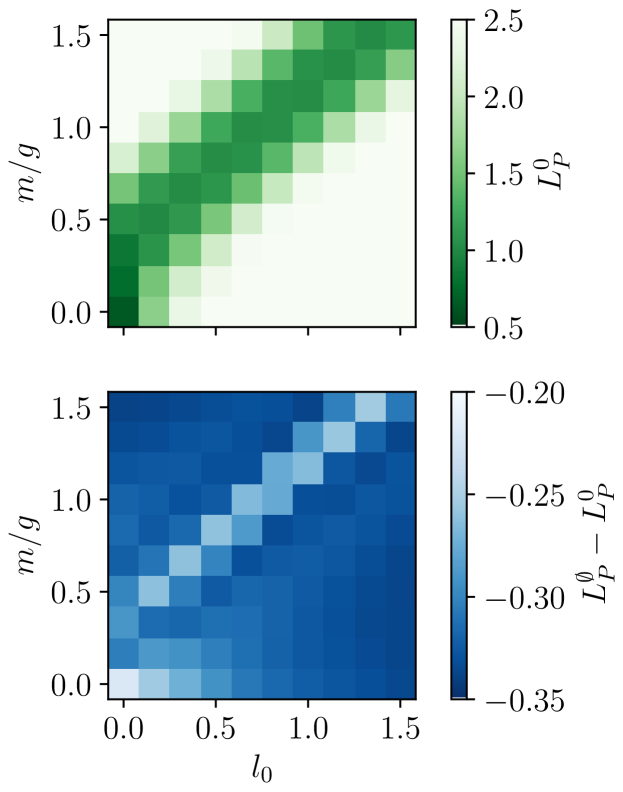
Figure 3: Top panel: improvement of the ZNE mitigation for the particle number $\expectationvalue{P}$ with respect to the ED evolution. Bottom panel: advantage of our method compared to the top panel.

Figure 3 shows, for the $P$ observable, a parameter scan of $10\times 10$ blocks over the region $(l_{0},m/g)\in[0,1.5]^{2}$ where it is computed, in the top panel, the error of ZNE with respect to the ED dynamics and, in the bottom panel, the improvement of our method with respect to ZNE. The top panel gives us the scale of the ZNE error, and the bottom panel tells us by how much that error was reduced within our BBGKY-improved scheme. A systematic improvement over the entire parameter-region is manifest by the presence of only negative $L^{\emptyset}_{P}-L^{0}_{P}$ values and, taking average values as in table 1, it is approximately $18.2\%$. The diagonal line in both panels can be explained by a system-dependent artifact caused by the alignment of the ED dynamics to the saturation, or flattening, of the measurements as in figure 4.

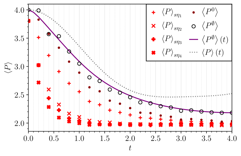
Figure 4: Evolution of the particle number $\expectationvalue{P}$ in the $(l_{0},m/g)=(0,0)$ regime. The red crosses are measurements at increasing noise levels, the dark red points are ZNEs, the black circles are BBGKY-improved ZNEs, the purple line is the Bernstein polynomial associated to the latter, and the dashed gray line is the ED evolution.

Figure 4 shows the time evolution of the $(l_{0},m/g)=(0,0)$ block of figure 3. We see that after ${\sim}15$ Trotter steps the measurements saturate, and recovering the original dynamics becomes challenging. Nevertheless, thanks to the additional BBGKY constraints, we see that the Bernstein polynomial correctly tries to match the time derivatives of the ED evolution.

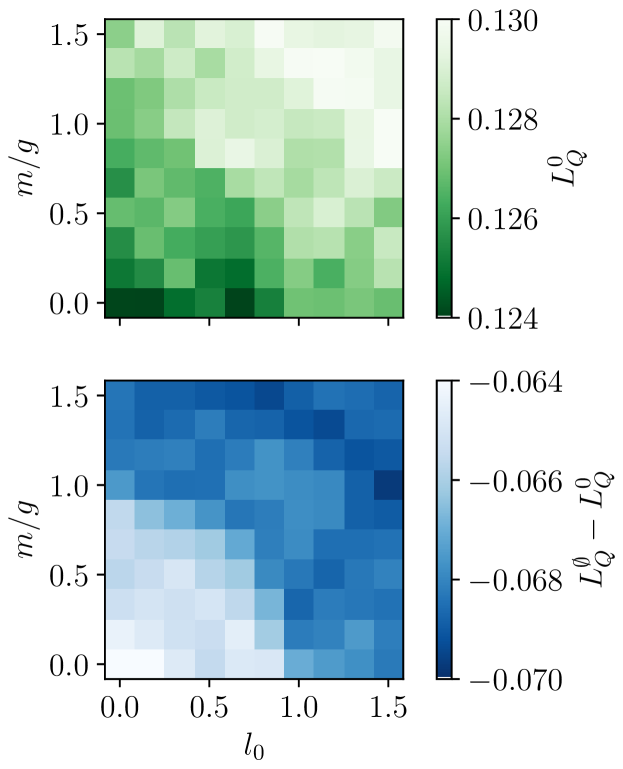
Figure 5: Top panel: improvement of the ZNE mitigation for the electric charge $\expectationvalue{Q}$ with respect to the ED evolution. Bottom panel: advantage of our method compared to the top panel.

Figure 5 shows the contents of figure 3 but for the $Q$ observable. Again, a systematic improvement over the entire parameter-region is observed with our method and, from table 1, we see that it is approximately $52.8\%$ with respect to ZNE. Here the bottom-left artifact region of the bottom panel can be explained by the small values of $(l_{0},m/g)$, reducing the importance of the BBGKY equations in the LLSQ minimization.

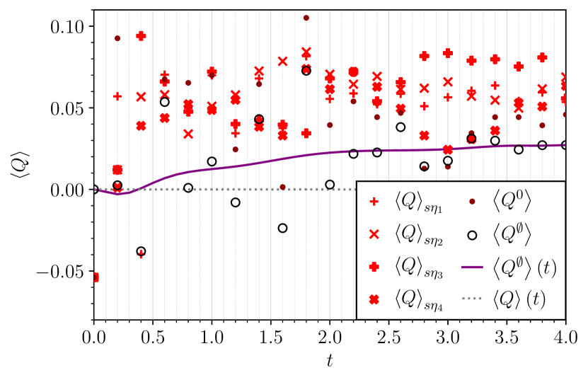
Figure 6: Evolution of the electric charge $\expectationvalue{Q}$ in the $(l_{0},m/g)=(0,0)$ regime. The same symbols and colors of figure 4 are used.

Figure 6 shows the time evolution of the $(l_{0},m/g)=(0,0)$ block of figure 5. Here, no saturation phenomenon occurs, because all measurements remain equally noisy. Nevertheless, thanks to the additional BBGKY constraints, we see again that the Bernstein polynomial correctly tries to match the null time derivative of the conserved quantity $Q$.

$\quad\,q\quad\,$	$L^{0}_{q}\,\,\,\text{(ZNE)}$	$L^{\emptyset}_{q}\,\,\,\text{(Ours)}$	$L^{\emptyset}_{q}-L^{0}_{q}$	$(L^{\emptyset}_{q}-L^{0}_{q})/L^{0}_{q}$
$P$	1.975	1.659	-0.316	-18.2%
$Q$	0.128	0.060	-0.068	-52.8%

Table 1: First column: average errors of ZNE against ED. Second column: average errors of our method against ED. Third column: absolute average improvements of our method against ZNE. Fourth column: relative average improvements of our method against ZNE. The averages for the $q=P,Q$ observables are computed, respectively, from the data of figures 3 and 5.

Table 1 summarizes as averages the errors, the absolute and the relative improvements of the previous two parameter scans, shown in figures 3 and 5. Again, with our method, we see a systematic improvement of the two mitigations with respect to ZNE, for both the non-conserved $P$ and the conserved $Q$, although we observe a larger relative improvement in the mitigation of $\expectationvalue{Q}$. This is because noise concentrates around the ED evolution in figure 6 so, in the minimization of the LLSQ problem, the Bernstein polynomial is less penalized in deviating from the ZNE to match the null time derivative of $\expectationvalue{Q}$.

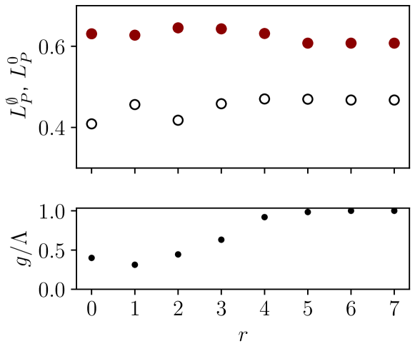
Figure 7: Top panel: errors for the mitigation of the particle number $\expectationvalue{P}$, in the $(l_{0},m/g)=(0,0)$ regime at different $r$, with ZNE (dark red points) and our method (black circles). Bottom panel: determination of the hierarchical subset.

We now study how the size of the selected subset of BBGKY equations affects the results of the mitigation. This is displayed in figure 7, where the mitigation of $\expectationvalue{P}$ in the $(l_{0},m/g)=(0,0)$ block is repeated for different maximal connections radii $r$. The top panel displays the errors of the ZNE and BBGKY-improved mitigations, while the bottom panel quantifies how many BBGKY equations $g$ cover the dynamics of the measured $\Lambda$ quantities.

A ratio of $g/\Lambda=1$, which is reached at $r=6$ and remains so at $r=7$, means that the subset of equations is fully determined with respect to its unknowns. In the present case $\Lambda=126<256=4^{N_{\text{Q}}}$, because the BBGKY hierarchy splits into 4 independent hierarchies of sizes 1, 1, 126 and 128. In particular, the two first hierarchies are composed, respectively, of solely the identity and $\sigma_{1}^{3}\sigma_{2}^{3}\sigma_{3}^{3}\sigma_{4}^{3}$, which are conserved quantities of (12). The third hierarchy involves $\{\sigma_{i}^{3}\}_{i\in S}$, which are required to build the conserved $Q$ observable.

We see that the inclusion of additional BBGKY constraints reduces the error with respect to ZNE immediately starting from $r=0$, in accordance with figure 3. In our experiments with the Schwinger model, no clear pattern regarding the reduction or the increase of absolute errors can be stated for $r>0$, neither in this $(l_{0},m/g)=(0,0)$ simulation nor in other different points of the parameter scan. We conjecture that a similar behavior is valid for other systems and therefore the optimal regime of our method lies close to a small $r=0$ hierarchical subset. This is because, given the ratio of the number of lines in the $M$ matrix distributed among ZNE and the BBGKY equations, the LLSQ problem prevents the Bernstein polynomial from deviating too much from the original ZNEs even as $g$ increases. Moreover, the number of time points $N$ may be too small for the Bernstein polynomial to benefit from its uniform convergence, leading to a systematic non-negligible additional approximation error from (6).

V Conclusions

In this paper, we considered executions of quantum algorithms as time evolutions of idealized systems. Their noiseless dynamics are governed by physical laws, which can be employed to mitigate the quantum errors arising from their physical realizations. For this purpose, we derived a corresponding BBGKY-like hierarchy and selected a $\text{poly}(N_{\text{Q}})$-large subset of its equations. We proposed a novel QEM scheme encapsulating these supplementary physics-informed constraints into the ZNE procedure. A LLSQ problem is thereby obtained, whose required classical computational resources scale polynomially in $N_{\text{Q}}$. We numerically investigated the effectiveness of our method on digital quantum simulations, mimicking realistic quantum hardware noise, of the lattice Schwinger model.

By applying our method to the lattice Schwinger model, we assessed our BBGKY-informed QEM scheme against ZNE by comparing the mitigation of quantum observables to known ED evolutions. It was found that, in the considered regions of the parameter scan and under the selected input parameters, our method systematically improves the QEM of ZNE measurements. Moreover, with our method, it was found that the range of relative improvement of the error with respect to ZNE spans from $18.2\%$ to $52.8\%$, depending on whether the mitigated quantity is conserved or not. It was found that the maximal connections radius of the selected hierarchical subset should be close to $r=0$, as such a subset of BBGKY equations already guarantees a systematic improvement over ZNE.

Further expansion of this work includes imaginary time evolution and evolution with time-dependent Hamiltonians. The latter would pave the way to the mitigation of adiabatic time evolution. This would also allow the mitigation of quantum circuits, if implemented as Trotterized time evolutions of a time-dependent system. Finally, the supplementary physical knowledge of the BBGKY hierarchy could be used to not only help ZNE but other mitigation schemes as well, either on digital or analog quantum machines. This could be done either as an entirely post-processing procedure, or directly affecting the parameters of quantum computation, as in variational methods.

Appendix A Upstream connected correlators

Here we derive an algorithm composed of three subroutines to obtain all $\sigma(A,(\mu_{k})_{k\in A})$ correlators upstream connected to the target $\sigma(B,(\nu_{k})_{k\in B})$. First, define the function $\bar{\varepsilon}(\mu,\nu):=\lambda\absolutevalue{\varepsilon_{\mu\nu\lambda}}$, where Einstein’s summation is still implied, to be interpreted as that index such that $\varepsilon_{\mu\nu\bar{\varepsilon}(\mu,\nu)}\neq 0$. Let also $n_{A}=\absolutevalue{A}$ and $n_{B}=\absolutevalue{B}$.

For the $n_{A}=n_{B}$ case, we observe in the second summation of (3) that, for $\sigma(B,(\nu_{k})_{k\in B})$ to appear in the expectation value, it must be $A=B$. Regarding the directions $(\mu_{k})_{k\in A}$, selecting an $i\in A$ ($n_{B}$ choices) and letting $\mu_{k}=\nu_{k}$ for all $k\in A\setminus\quantity{i}$, we see that if we want $\nu$ to pick up the desired $\nu=\nu_{i}$ value then, because of the Levi-Civita symbol, it must be $\mu_{i}\neq\nu_{i}$ (2 choices). Then $\lambda=\bar{\varepsilon}(\mu_{i},\nu_{i})$, hence $\sigma(B,(\nu_{i})_{i\in B})$ appears in the second summation only if

$$h_{i}^{\bar{\varepsilon}(\mu_{i},\nu_{i})}\neq 0.$$ (16)

In total, $2n_{B}$ possible $\sigma(A,(\mu_{k})_{k\in A})$ ansätze have to be checked against the magnetic field.

For the $n_{A}=n_{B}-1$ case, we observe in the third summation of (3) that, for $\sigma(B,(\nu_{k})_{k\in B})$ to appear in the expectation value, it must be $A=B\setminus\quantity{j}$ for a selected $j\in B$ ($n_{B}$ choices). Regarding the directions $(\mu_{k})_{k\in A}$, selecting a specific $i\in A$ ($n_{B}-1$ choices) and letting $\mu_{k}=\nu_{k}$ for all $k\in A\setminus\quantity{i}$, we see that if we want $\lambda$ to pick up the desired $\lambda=\nu_{i}$ value then, again because of the Levi-Civita symbol, it must be $\mu_{i}\neq\nu_{i}$ (2 choices). Then $\mu=\bar{\varepsilon}(\mu_{i},\nu_{i})$, hence $\sigma(B,(\nu_{k})_{k\in B})$ appears in the third summation only if

$$V_{ij}^{\bar{\varepsilon}(\mu_{i},\nu_{i})\nu_{j}}\neq 0.$$ (17)

Notice that the index $\nu$ will necessarily pick $\nu=\nu_{j}$ because it is contracted independently. In total, $2n_{B}(n_{B}-1)$ possible $\sigma(A,(\mu_{k})_{k\in A})$ ansätze have to be checked against the interaction potential.

For the $n_{A}=n_{B}+1$ case, we observe in the first summation of (3) that, for $\sigma(B,(\nu_{k})_{k\in B})$ to appear in the expectation value, it must be $A=B\cup\quantity{i}$ for a selected $i\in S\setminus B$ ($N_{\text{Q}}-n_{B}$ choices). Regarding the directions $(\mu_{k})_{k\in A}$, selecting a specific $j\in B$ ($n_{B}$ choices) and letting $\mu_{k}=\nu_{k}$ for all $k\in A\setminus\quantity{i,j}$ and $\mu_{i}\in\quantity{1,2,3}$ (3 choices), we see that if we want $\lambda$ to pick up the desired $\lambda=\nu_{j}$ value then, once again because of the Levi-Civita symbol, it must be $\mu_{j}\neq\nu_{j}$ (2 choices). Then $\nu=\bar{\varepsilon}(\mu_{j},\nu_{j})$, hence $\sigma(B,(\nu_{k})_{k\in B})$ appears in the first summation only if

$$V_{ij}^{\mu_{i}\bar{\varepsilon}(\mu_{j},\nu_{j})}\neq 0.$$ (18)

In total, $6n_{B}(N_{\text{Q}}-n_{B})$ possible $\sigma(A,(\mu_{k})_{k\in A})$ ansätze have to be checked against the interaction potential.

To sum things up, there is a polynomial in $n_{B}$ and $N_{\text{Q}}$ amount of ansätze to check against the coefficients of (2), and the number of checks is overall bounded by $9N_{\text{Q}}^{2}/4$.

Appendix B Random shift of error levels

Every time (4) is employed to measure a $(\varepsilon_{s\eta},\expectationvalue{Q_{q}}_{s\eta})$ data point, a small random shift $\varepsilon_{s\eta}\to\varepsilon_{s\eta}+\chi$ is performed, where $\chi$ is a realization of the normally distributed random variable $X\sim\mathcal{N}(0,1/N_{\text{S}})$. This is to avoid cases where two different noise levels $\eta_{1}\neq\eta_{2}$ produce the same error level, for example $\eta_{1}=1$ and $\eta_{2}=1.5$ leading to $\varepsilon_{1\eta_{1}}=\varepsilon_{1\eta_{2}}=3$, thereby introducing artifacts in the LSP interpolation. The variance of $X$ is chosen to be $1/N_{\text{S}}$ to mimic the standard deviation estimator when $N_{\text{S}}\to\infty$ and also because, in that limit, the $\chi$ shift shouldn’t affect $\varepsilon_{s\eta}$, as quantum errors had an infinite $N_{\text{S}}\to\infty$ amount of possibilities to arise.

Appendix C Example of an $M$ matrix

To illustrate the construction of $M$ with a simple yet non-trivial example, consider the mitigation of $l=\Lambda=2$ quantities after $N=2$ Trotter steps with the $g=2$ fictitious BBGKY equations

$$\derivative{t}\expectationvalue{Q_{0}}=0\qquad\text{and}\qquad\derivative{t}\expectationvalue{Q_{1}}=V\expectationvalue{Q_{0}},$$ (19)

where $V\neq 0$ is constant and $Q_{0},Q_{1}$ are, respectively, $n$-point and $(n+1)$-point correlators. Then, in this example, the $\overrightarrow{\mathbf{v}}$ vector is given by  
cell-space-limits = 2.5pt

$$\overrightarrow{\mathbf{v}}(\overrightarrow{\mathbf{a}})\,=\,\,\pNiceMatrix[r,margin,first-col]\Block{3-1}{M_{1\overrightarrow{\mathbf{\eta}}}\quad\,}&\Block[borders={right,tikz=dashed}]{18-6}{}\Block[borders={top,bottom,left,tikz=dashed}]{6-6}{}\Block[borders={right,bottom,tikz=dotted}]{3-3}{}\varepsilon_{1\eta_{1}}^{d}\Cdots 1\\ \Vdots\Ddots\Vdots\\ \varepsilon_{1\eta_{m}}^{d}\Cdots 1\\ \Block{3-1}{M_{2\overrightarrow{\mathbf{\eta}}}\quad\,}\Block[borders={top,left,tikz=dotted}]{3-3}{}\varepsilon_{2\eta_{1}}^{d}\Cdots 1\\ \Vdots\Ddots\Vdots\\ \varepsilon_{2\eta_{m}}^{d}\Cdots 1\\ \Block{3-1}{M_{1\overrightarrow{\mathbf{\eta}}}\quad\,}\Block[borders={top,right,tikz=dashed}]{6-6}{}\Block[borders={right,bottom,tikz=dotted}]{3-3}{}\varepsilon_{1\eta_{1}}^{d}\Cdots 1\\ \Vdots\Ddots\Vdots\\ \varepsilon_{1\eta_{m}}^{d}\Cdots 1\\ \Block{3-1}{M_{2\overrightarrow{\mathbf{\eta}}}\quad\,}\Block[borders={top,left,tikz=dotted}]{3-3}{}\varepsilon_{2\eta_{1}}^{d}\Cdots 1\\ \Vdots\Ddots\Vdots\\ \Block[borders={bottom,tikz=solid}]{1-12}{}\varepsilon_{2\eta_{m}}^{d}\Cdots 1\\ \par\par\Block{6-1}{G\quad\,}\Block[borders={right,tikz=dotted}]{6-3}{}\Block[r]{1-3}{\beta_{12}(0)}\Block[r]{1-3}{\beta_{22}(0)}\Block[borders={right,tikz=dotted}]{6-3}{}\Block[r]{1-3}{}\\ \par\par\Block[r]{1-3}{\beta_{12}(\frac{1}{2})}\Block[r]{1-3}{\beta_{22}(\frac{1}{2})}\Block[r]{1-3}{}\\ \par\Block[r]{1-3}{\beta_{12}(1)}\Block[r]{1-3}{\beta_{22}(1)}\Block[r]{1-3}{}\\ \par\Block[borders={top,tikz=solid}]{1-12}{}\par\Block[r]{1-3}{\beta_{12}(0)}\Block[r]{1-3}{\beta_{22}(0)}\\ \par\Block[r]{1-3}{-V}\Block[r]{1-3}{\beta_{12}(\frac{1}{2})}\Block[r]{1-3}{\beta_{22}(\frac{1}{2})}\\ \par\Block[r]{1-3}{-V}\Block[r]{1-3}{\beta_{12}(1)}\Block[r]{1-3}{\beta_{22}(1)}\\ \par\CodeAfter\OverBrace[yshift=5pt]{1-1}{1-6}{Q_{0}}\OverBrace[yshift=5pt]{1-7}{1-12}{Q_{1}}\OverBrace[yshift=5pt]{7-7}{7-9}{t_{1}}\OverBrace[yshift=5pt]{7-10}{7-12}{t_{2}}\UnderBrace[yshift=5pt]{6-1}{6-3}{t_{1}}\UnderBrace[yshift=5pt]{6-4}{6-6}{t_{2}}\SubMatrix{.}{1-1}{3-1}{\{}[xshift=-14mm]\SubMatrix{.}{4-1}{6-1}{\{}[xshift=-14mm]\SubMatrix{.}{7-1}{9-1}{\{}[xshift=-14mm]\SubMatrix{.}{10-1}{12-1}{\{}[xshift=-14mm]\SubMatrix{.}{13-1}{18-1}{\{}[xshift=-14mm]\UnderBrace[yshift=5pt]{1-1}{last-last}{M}\,\cdot\,\,\pNiceMatrix[last-col]a_{01d}&\Block{3-1}{\quad\overrightarrow{\mathbf{a}}_{01}}\\ \Vdots\\ \Block[borders={bottom,tikz=dotted}]{1-1}{}\expectationvalue*{Q^{\emptyset}_{0}}_{1}\\ a_{02d}\Block{3-1}{\quad\overrightarrow{\mathbf{a}}_{02}}\\ \Vdots\\ \Block[borders={bottom,tikz=dashed}]{1-1}{}\expectationvalue*{Q^{\emptyset}_{0}}_{2}\\ a_{11d}\Block{3-1}{\quad\overrightarrow{\mathbf{a}}_{11}}\\ \Vdots\\ \Block[borders={bottom,tikz=dotted}]{1-1}{}\expectationvalue*{Q^{\emptyset}_{1}}_{1}\\ a_{12d}\Block{3-1}{\quad\overrightarrow{\mathbf{a}}_{12}}\\ \Vdots\\ \expectationvalue*{Q^{\emptyset}_{1}}_{2}\CodeAfter\SubMatrix{.}{1-1}{3-last}{\}}[xshift=2.5mm]\SubMatrix{.}{4-1}{6-last}{\}}[xshift=2.5mm]\SubMatrix{.}{7-1}{9-last}{\}}[xshift=2.5mm]\SubMatrix{.}{10-1}{last-last}{\}}[xshift=2.5mm]\UnderBrace[yshift=3pt]{last-1}{last-last}{\overrightarrow{\mathbf{a}}}-\quad\pNiceMatrix[last-col]\expectationvalue*{Q_{0}}_{1\eta_{1}}&\Block{3-1}{\quad\overrightarrow{\mathbf{y}}_{01\overrightarrow{\mathbf{\eta}}}}\\ \Vdots\\ \Block[borders={bottom,tikz=dotted}]{1-1}{}\expectationvalue*{Q_{0}}_{1\eta_{m}}\\ \expectationvalue*{Q_{0}}_{2\eta_{1}}\Block{3-1}{\quad\overrightarrow{\mathbf{y}}_{02\overrightarrow{\mathbf{\eta}}}}\\ \Vdots\\ \Block[borders={bottom,tikz=dashed}]{1-1}{}\expectationvalue*{Q_{0}}_{2\eta_{m}}\\ \expectationvalue*{Q_{1}}_{1\eta_{1}}\Block{3-1}{\quad\overrightarrow{\mathbf{y}}_{11\overrightarrow{\mathbf{\eta}}}}\\ \Vdots\\ \Block[borders={bottom,tikz=dotted}]{1-1}{}\expectationvalue*{Q_{1}}_{1\eta_{m}}\\ \expectationvalue*{Q_{1}}_{2\eta_{1}}\Block{3-1}{\quad\overrightarrow{\mathbf{y}}_{12\overrightarrow{\mathbf{\eta}}}}\\ \Vdots\\ \Block[borders={bottom,tikz=solid}]{1-1}{}\expectationvalue*{Q_{1}}_{2\eta_{m}}\\ -\beta_{02}(0)\expectationvalue*{Q^{\emptyset}_{0}}_{0}\Block{6-1}{\quad\overrightarrow{\mathbf{g}}}\\ -\beta_{02}(\frac{1}{2})\expectationvalue*{Q^{\emptyset}_{0}}_{0}\\ \Block[borders={bottom,tikz=solid}]{1-1}{}-\beta_{02}(1)\expectationvalue*{Q^{\emptyset}_{0}}_{0}\\ \quantity(V-\beta_{02}(0))\expectationvalue*{Q^{\emptyset}_{1}}_{0}\\ -\beta_{02}(\frac{1}{2})\expectationvalue*{Q^{\emptyset}_{1}}_{0}\\ -\beta_{02}(1)\expectationvalue*{Q^{\emptyset}_{1}}_{0}\CodeAfter\SubMatrix{.}{1-1}{3-last}{\}}[xshift=2.5mm]\SubMatrix{.}{4-1}{6-last}{\}}[xshift=2.5mm]\SubMatrix{.}{7-1}{9-last}{\}}[xshift=2.5mm]\SubMatrix{.}{10-1}{12-last}{\}}[xshift=2.5mm]\SubMatrix{.}{13-1}{18-last}{\}}[xshift=2.5mm]\UnderBrace[yshift=3pt]{last-1}{last-last}{\overrightarrow{\mathbf{y}}}\;.$$ (20)

References

- Shor [1995] P. W. Shor, Scheme for reducing decoherence in quantum computer memory, Phys. Rev. A 52, R2493 (1995).
- Steane [1996] A. M. Steane, Error Correcting Codes in Quantum Theory, Phys. Rev. Lett. 77, 793 (1996).
- Calderbank and Shor [1996] A. R. Calderbank and P. W. Shor, Good quantum error-correcting codes exist, Phys. Rev. A 54, 1098 (1996).
- Nielsen and Chuang [2010] M. A. Nielsen and I. L. Chuang, Quantum Computation and Quantum Information: 10th Anniversary Edition (Cambridge University Press, 2010).
- Chatterjee et al. [2024] A. Chatterjee, A. Ghosh, and S. Ghosh, Quantum Prometheus: Defying Overhead with Recycled Ancillas in Quantum Error Correction, (2024), arXiv:2411.12813 [quant-ph] .
- Ezzell et al. [2023] N. Ezzell, B. Pokharel, L. Tewala, G. Quiroz, and D. A. Lidar, Dynamical decoupling for superconducting qubits: A performance survey, Phys. Rev. Appl. 20, 064027 (2023).
- Wallman and Emerson [2016] J. J. Wallman and J. Emerson, Noise tailoring for scalable quantum computation via randomized compiling, Phys. Rev. A 94, 052325 (2016).
- van den Berg et al. [2022] E. van den Berg, Z. K. Minev, and K. Temme, Model-free readout-error mitigation for quantum expectation values, Phys. Rev. A 105, 032620 (2022).
- Temme et al. [2017] K. Temme, S. Bravyi, and J. M. Gambetta, Error Mitigation for Short-Depth Quantum Circuits, Phys. Rev. Lett. 119, 180509 (2017).
- Giurgica-Tiron et al. [2020] T. Giurgica-Tiron, Y. Hindy, R. LaRose, A. Mari, and W. J. Zeng, Digital zero noise extrapolation for quantum error mitigation, in 2020 IEEE International Conference on Quantum Computing and Engineering (2020) arXiv:2005.10921 [quant-ph] .
- Endo et al. [2018] S. Endo, S. C. Benjamin, and Y. Li, Practical Quantum Error Mitigation for Near-Future Applications, Phys. Rev. X 8, 031027 (2018).
- Strikis et al. [2021] A. Strikis, D. Qin, Y. Chen, S. C. Benjamin, and Y. Li, Learning-Based Quantum Error Mitigation, PRX Quantum 2, 040330 (2021).
- Kim et al. [2020] C. Kim, K. Park, and J. Rhee, Quantum error mitigation with artificial neural network, IEEE Access 8, 18853 (2020).
- Cai et al. [2020] Z. Cai, X. Xu, and S. C. Benjamin, Mitigating coherent noise using Pauli conjugation, npj Quantum Inf. 6, 17 (2020).
- Takagi et al. [2022] R. Takagi, S. Endo, S. Minagawa, and M. Gu, Fundamental limits of quantum error mitigation, npj Quantum Information 8, 114 (2022).
- Quek et al. [2024] Y. Quek, D. Stilck França, S. Khatri, J. J. Meyer, and J. Eisert, Exponentially tighter bounds on limitations of quantum error mitigation, Nature Physics 20, 1648 (2024).
- Pomarico et al. [2025] D. Pomarico, M. Pandey, R. Cioli, F. Dell’Anna, S. Pascazio, F. V. Pepe, P. Facchi, and E. Ercolessi, Quantum error mitigation in optimized circuits for particle-density correlations in real-time dynamics of the Schwinger model, (2025), arXiv:2501.10831 [quant-ph] .
- Suzuki et al. [2022] Y. Suzuki, S. Endo, K. Fujii, and Y. Tokunaga, Quantum Error Mitigation as a Universal Error Reduction Technique: Applications from the NISQ to the Fault-Tolerant Quantum Computing Eras, PRX Quantum 3, 010345 (2022).
- Zimborás et al. [2025] Z. Zimborás et al., Myths around quantum computation before full fault tolerance: What no-go theorems rule out and what they don’t, (2025), arXiv:2501.05694 [quant-ph] .
- Zhang et al. [2025] A. Zhang et al., Demonstrating quantum error mitigation on logical qubits, (2025), arXiv:2501.09079 [quant-ph] .
- Bonet-Monroig et al. [2018] X. Bonet-Monroig, R. Sagastizabal, M. Singh, and T. E. O’Brien, Low-cost error mitigation by symmetry verification, Phys. Rev. A 98, 062339 (2018).
- Smart and Mazziotti [2019] S. E. Smart and D. A. Mazziotti, Quantum-classical hybrid algorithm using an error-mitigating N-representability condition to compute the Mott metal-insulator transition, Phys. Rev. A 100, 022517 (2019).
- Bogoliubov [1946] N. N. Bogoliubov, Kinetic Equations, Journal of Physics-USSR 10, 265 (1946).
- Born and Green [1946] M. Born and H. S. Green, A General Kinetic Theory of Liquids. I. The Molecular Distribution Functions, Proc. Roy. Soc. Lond. A 188, 10 (1946).
- Kirkwood [1946] J. G. Kirkwood, The Statistical Mechanical Theory of Transport Processes I. General Theory, The Journal of Chemical Physics 14, 180 (1946).
- Yvon [1935] J. Yvon, La théorie statistique des fluides et l’équation d’état, Actualités scientifiques et industrielles : hydrodynamique, acoustique: Théories mécaniques (Hermann & cie, 1935).
- Chari et al. [2016] S. Chari, R. Inguva, and K. Murthy, A new truncation scheme for BBGKY hierarchy: conservation of energy and time reversibility, arXiv preprint arXiv:1608.02338 (2016).
- Pucci et al. [2016] L. Pucci, A. Roy, and M. Kastner, Simulation of quantum spin dynamics by phase space sampling of Bogoliubov-Born-Green-Kirkwood-Yvon trajectories, Phys. Rev. B 93, 174302 (2016).
- Paškauskas and Kastner [2012] R. Paškauskas and M. Kastner, Equilibration in long-range quantum spin systems from a BBGKY perspective, Journal of Statistical Mechanics: Theory and Experiment 2012, P02005 (2012).
- Lacroix et al. [2016] D. Lacroix, Y. Tanimura, S. Ayik, and B. Yilmaz, A simplified BBGKY hierarchy for correlated fermions from a stochastic mean-field approach, The European Physical Journal A 52, 1 (2016).
- Li and Benjamin [2017] Y. Li and S. C. Benjamin, Efficient Variational Quantum Simulator Incorporating Active Error Minimization, Phys. Rev. X 7, 021050 (2017), arXiv:1611.09301 [quant-ph] .
- Schwinger [1962] J. Schwinger, Gauge Invariance and Mass. II, Phys. Rev. 128, 2425 (1962).
- Angelides et al. [2025] T. Angelides, P. Naredi, A. Crippa, K. Jansen, S. Kühn, I. Tavernelli, and D. S. Wang, First-order phase transition of the Schwinger model with a quantum computer, npj Quantum Inf. 11, 6 (2025), arXiv:2312.12831 [hep-lat] .
- Honda et al. [2022] M. Honda, E. Itou, Y. Kikuchi, L. Nagano, and T. Okuda, Classically emulated digital quantum simulation for screening and confinement in the Schwinger model with a topological term, Phys. Rev. D 105, 014504 (2022).
- Pederiva et al. [2022] G. Pederiva, A. Bazavov, B. Henke, L. Hostetler, D. Lee, H.-W. Lin, and A. Shindler, Quantum State Preparation for the Schwinger Model, PoS LATTICE2021, 047 (2022).
- Yamamoto [2022] A. Yamamoto, Toward dense QCD in quantum computers, PoS LATTICE2021, 122 (2022).
- Chakraborty et al. [2022] B. Chakraborty, M. Honda, T. Izubuchi, Y. Kikuchi, and A. Tomiya, Classically emulated digital quantum simulation of the Schwinger model with a topological term via adiabatic state preparation, Phys. Rev. D 105, 094503 (2022).
- Ghim and Honda [2024] D. Ghim and M. Honda, Digital Quantum Simulation for Spectroscopy of Schwinger Model, PoS LATTICE2023, 213 (2024), arXiv:2404.14788 [hep-lat] .
- Kaikov et al. [2024] O. Kaikov, T. Saporiti, V. Sazonov, and M. Tamaazousti, Phase Diagram of the Schwinger Model by Adiabatic Preparation of States on a Quantum Simulator, (2024), arXiv:2407.09224 [hep-lat] .
- D’Anna et al. [2024] M. D’Anna, M. Krstic Marinkovic, and J. C. P. Barros, Adiabatic state preparation for digital quantum simulations of QED in 1 + 1D, (2024), arXiv:2411.01079 [hep-lat] .
- Cox and Stamp [2018] T. Cox and P. C. E. Stamp, Partitioned density matrices and entanglement correlators, Phys. Rev. A 98, 062110 (2018).
- Trotter [1959] H. F. Trotter, On the Product of Semi-Groups of Operators, Proceedings of the American Mathematical Society 10, 545 (1959).
- Berry et al. [2007] D. W. Berry, G. Ahokas, R. Cleve, and B. C. Sanders, Efficient Quantum Algorithms for Simulating Sparse Hamiltonians, Commun. Math. Phys. 270, 359 (2007), arXiv:quant-ph/0508139 .
- Hatano and Suzuki [2005] N. Hatano and M. Suzuki, Finding Exponential Product Formulas of Higher Orders, Lect. Notes Phys. 679, 37 (2005), arXiv:math-ph/0506007 .
- Magnus [1954] W. Magnus, On the exponential solution of differential equations for a linear operator, Commun. Pure Appl. Math. 7, 649 (1954).
- Note [1] We systematically add a small random shift to for reasons explained in appendix B.
- Floater [2005] M. S. Floater, On the convergence of derivatives of Bernstein approximation, Journal of Approximation Theory 134, 130 (2005).
- S. Bernstein [1913] S. Bernstein, Démonstration du théorème de Weierstrass fondée sur le calcul des probabilités, Communications of the Kharkov Mathematical Society XIII, 2 (1913).
- Kogut and Susskind [1975] J. B. Kogut and L. Susskind, Hamiltonian Formulation of Wilson’s Lattice Gauge Theories, Phys. Rev. D 11, 395 (1975).
- Jordan and Wigner [1928] P. Jordan and E. P. Wigner, About the Pauli exclusion principle, Z. Phys. 47, 631 (1928).
- Javadi-Abhari et al. [2024] A. Javadi-Abhari, M. Treinish, K. Krsulich, C. J. Wood, J. Lishman, J. Gacon, S. Martiel, P. D. Nation, L. S. Bishop, A. W. Cross, B. R. Johnson, and J. M. Gambetta, Quantum computing with Qiskit (2024), arXiv:2405.08810 [quant-ph] .
- Note [2] The simulations for were conducted on February 4th 2025 while those for on February 5th 2025.