Abstract

We study bifurcations from the cylinder governed by the Helfrich equation. The bifurcating solutions are in three classes, axisymmetric, non axisymmetric without Gaussian curvature and completely non axisymmetric solutions. Depending on the spontaneous curvature we find stability regimes of the cylinder and destabilizing bifurcations to spatially periodic solutions. To get a complete picture we use well established local bifurcation methods. Numerical continuation provides global stability statements of the bifurcations.

1 Introduction

We consider the Helfrich equation

$$\dot{X}=\left(\Delta H+2H(H^{2}-K)+2c_{0}K-2(c_{0}^{2}+\lambda_{1})H-\lambda_{2}\right)N,$$ (1)

with $c_{0}$ the spontaneous (or preferred curvature) and $\Lambda:=(\lambda_{1},\lambda_{2})$ are Lagrange multipliers for the area and the volume, respectively. The cylinder $\mathcal{C}_{r}$ of radius $r$ is a stationary solution to (1) iff

$$\lambda_{1}=\frac{1}{2}\left(\frac{1}{2r^{2}}-2r\lambda_{2}-2c_{0}^{2}\right).$$ (2)

Typically for compact manifolds the integral

$$E(X,c_{0})=\int_{X}a(H-c_{0})^{2}+bK\,{\rm d}S$$ (3)

is called the Helfrich energy. The area of such manifold is define by

$${\cal A}(X):=\int_{X}\,{\rm d}S$$ (4)

and for cylindrical surfaces the volume is

$${\cal V}(X)=\frac{1}{2}\int_{X}\frac{(r+u)^{2}}{g^{1/2}}\,{\rm d}S=\frac{1}{2}\int_{I\times\mathbb{S}^{1}}(r+u)^{2}\,{\rm d}(x,\varphi).$$ (5)

First introduced in [Hel73], for compact manifolds an area and volume constraint was introduced, leading to the Lagrangian

$$F(X,c_{0})=E(X,c_{0})+\lambda_{1}({\cal A}(X)-{\cal A}_{0})+\lambda_{2}({\cal V}(X)-{\cal V}_{0}),$$ (6)

with Euler-Lagrange equation (1) with $a=1$ and $b=0$, for variation in normal direction of $X$. In the case with boundary additional boundary terms come up, defining natural boundary conditions, [PP22]. But in the case of $\mathcal{C}_{r}$ the energy is not well defined, rather on each compact portion of length $L$, call this $\mathcal{C}_{r}(L)$. However on $\mathcal{C}_{r}(L)$ we have a scaling, that for $E(\mathcal{C}_{\alpha r}(L),c_{0})=E(\mathcal{C}_{r}(\alpha L),c_{0}/\alpha)$. So near a compact cylinder, it is sufficient to consider $r=1$ with a variable length and abbreviate $\mathcal{C}=\mathcal{C}_{1}$.

Associated to (6) is a $L^{2}$-gradient flow of the form

$$\begin{pmatrix}V_{t}:=\left\langle\dot{X},N(t)\right\rangle\\ 0\end{pmatrix}=\begin{pmatrix}G(X(t),\Lambda)\\ q(X(t))\end{pmatrix},\quad q(X(t))=\begin{pmatrix}{\cal A}(X(t))-{\cal A}_{0}\\ {\cal V}(X(t))-{\cal V}_{0}\end{pmatrix}$$ (7)

where $G(X(t),\Lambda)$ is the rhs of (1) and $\lambda_{1}(t)$ and $\lambda_{2}(t)$ are time depending functions, such that the constraints for ${\cal A}(X)$ and ${\cal V}(X)$ are fulfilled. We will prove well-posedness result of (7) for initial conditions $X_{0}$ close to $\mathcal{C}_{r}$ + global existence.

1.1 Introductory example

For our first observation we use the continuation package pde2path, especially with the functions of the Xcont library. For short review of the numerical procedure see subsection A.1 and for a complete introduction see [MU24]. In our first experiments we try to capture the influence of the bifurcation wrt $c_{0}$. We use periodic boundary conditions, where the period sufficiently large ($L=10$) to detect primary bifurcation in the periodic boundary conditions. Neumann typ boundary conditions would also be a reasonable choice. The first test value is $c_{0}=0$ with the focus in the stability of the cylinder and destabilizing bifurcations. However an extended bifurcation diagram is discussed in section 5.

(a)	(b)

Figure 1: Bifurcation diagram (a) of (1) for the case $L=10$ and $c_{0}=0$. With sample solutions in (b) for the first bifurcation 0-BP1 in dark red to an axisymmetric branch. Then two branches bifurcating from 0-BP2 to the unstable spot like on the orange and stable spiral (strip like) solutions on the green branch.

For a given $r$ and $c_{0}$ equation (2) describes a family of active parameter vector $(\Lambda,V)$ on the trivial branch, with $V=V_{0}$. While the notion of stability will discussed rigorously in section 2, we shall comment on that now. We will consider the Helfrich flow projected on area and volume preservation. The parameters $\lambda_{i}$ are the Lagrange multipliers to the area and volume constraint. Hence in the dynamical problem (7) the $\lambda_{i}$’s are functions of $t$ to ensure the constraints. In the continuation the stability is calculated for a fixed primary continuation parameter, hence stability information is not valid if $\lambda_{i}$’s are primary. However we can easily change the parameter vector, e.g. to $(V,\Lambda)$ for the eigenvalue calculation and the detection of the bifurcation points, while volume change along the bifurcating branch ins allowed. Due to the scale invariance of (3) on the cylinder and the two constraints we introduce the reduced volume as a uniform parameter describing the phase diagram, for more details see section 5.

Remark .

This point of view of allow the reduced volume to change along the branch, while considering volume preserving stability information is mainly motivated by the closed vesicle situation discussed for example in [JSR93]. Roughly s peaking the sphere is the unique optimum of maximal volume by minimal area. Hence volume and area preserving branches from the sphere do not exist. However the cylinder can be destabilized preserving the area and the volume while changing the langth noticed already in [ZcH89].

The first samples are done with $c_{0}=0$ presented in Figure 1. We find a narrow range of stability of the trivial branch 0, with two branch points at the end. At 0-BP1 (first number corresponds to the value of $c_{0}$) with $\lambda_{1}\approx?$ the bifurcating branch is axisymmetric. In contrast to the surface diffusion flow and considerations in [LS13] constant mean curvature surfaces of revolution are not solutions to (1) with $c_{0}=0$. For $c_{0}\neq 0$ this case can happen if $c_{0}=H(X)$. 0-BP1 has multiplicity two, corresponding to a translation of $L/4$ in $x$ direction and the bifurcation is a supercritical pitchfork, with the hidden symmetry that translation of $L/2$ corresponds to the other direction of the pitchfork.
The second destabilization 0-BP2 lead to a non-axisymmetric solution with axial wave number 1. However due to the symmetry of the kernel solutions 0-BP2 has multiplicity 4. with kernel function, rotated and translated. Due to the high multiplicity two branches bifurcate a corkscrews branch being stable and a wave like branch unstable.

1.2 Organization

First we shall set up the necessary differential geometry and rewrite(7) as an equation in the normal displacement of the cylinder. This gives a constrained gradient flow in $u$ associate with (3). In contrast to many others we establish maximal regularity of the parabolic problem in Sobolev spaces. This gives a short time of the flow. Due to the translation invariance of $\mathcal{C}_{r}$ close to the cylinder there is a two dimensional center manifold of cylinders with the same radius.
Again using the maximal regularity we can utilize the abstract result from Simonett und so that nonlinear stability follows from linearized stability. Since $\mathcal{C}_{r}$ has constant mean and Gauß curvature, the eigenvalues and eigenfunctions of the linearized stationary problem can be computed explicitly. Hence we derive the amplitude equations With this characterization we can prove the

2 Preliminaries and well-posedness of the flow

We introduce the basic differential geometric preliminaries in order to write (7) as a constrained parabolic quasi-linear equation in the normal displacement $u$ of the cylinder. This construction is as in [LS16], and hence we refrain from extensive computational details and focus on the structure and mapping properties of the resulting equations. From these we obtain maximal regularity results and hence local existence for (7). For general background on differential geometry we recommend [Tapp16, UY17].

2.1 Preliminaries

Let ${\cal C}(r)$ be the two dimensional unbounded cylinder embedded in ${\mathbb{R}}^{3}$ of radius $r>0$ with the unbounded direction along the $x$ axis. ${\cal C}(r)$ can be considered as the embedding

$$\begin{array}[]{rl}\Phi:{\mathbb{R}}\times\T&\rightarrow{\mathbb{R}}^{3}\\ (x,\varphi)&\mapsto\begin{pmatrix}x,r\cos(\varphi),r\sin(\varphi)\end{pmatrix}^{T}\end{array}$$ (10)

of the product manifold ${\mathbb{R}}\times\T$, where $\T$ is the one dimensional topological torus with length $2\pi$ endowed with the metric $d_{\T}(\varphi,\vartheta)=\min\{|\varphi-\vartheta|,2\pi-|\varphi-\vartheta|\}$ for all $\varphi,\vartheta\in\T$. Then as the pullback metric of the ${\mathbb{R}}^{3}$ to ${\cal C}(r)$ we have $g_{0}=\,{\rm d}x^{2}+r^{2}\,{\rm d}\varphi^{2}$. The normal vector (field) $N$ of ${\cal C}(r)$ is oriented inwards, wrt $\Phi$, hence $H({\cal C}_{r})=\frac{1}{2r}$.

For a function $u:{\cal C}(r)\rightarrow{\mathbb{R}}$, for the remainder of this subsection assumed as smooth as necessary, we consider surfaces

$$X={\cal C}(r)-u\,N,$$

assuming $u<r$, such that $X$ is still an embedding of ${\mathbb{R}}\times\T$; explicitly,

$$\tilde{\Phi}(x,\varphi)=\Phi(x,\varphi)+\tilde{u}(x,\varphi)(0,\cos(\varphi),\sin(\varphi))^{T},$$

where $\tilde{u}=u\circ\Phi$. This gives the metric

$$(g_{ij})=\begin{pmatrix}1+u_{x}^{2}&u_{x}u_{\varphi}\\ u_{x}u_{\varphi}&(r+u)^{2}+u^{2}_{\varphi}\end{pmatrix}\quad\text{with inverse }(g^{ij})=\frac{1}{g}\begin{pmatrix}(r+u)^{2}+u^{2}_{\varphi}&-u_{x}u_{\varphi}\\ -u_{x}u_{\varphi}&1+u_{x}^{2}\end{pmatrix}$$

with $g=\det(g_{ij})=(r+u)^{2}(1+u_{x}^{2})+u_{\varphi}^{2}$. In the same explicit fashion one can calculate the second fundamental form

$$(h_{ij})=\frac{1}{\sqrt{g}}\begin{pmatrix}(r+u)u_{xx}&(r+u)u_{x\varphi}-u_{x}u_{\varphi}\\ (r+u)u_{x\varphi}-u_{x}u_{\varphi}&(r+u)(u_{\varphi\varphi}-(r+u))-2u_{\varphi}^{2}\end{pmatrix},$$

and this gives explicit formulas for the mean and Gaussian curvatures,

$$H(u) =\frac{1}{2g^{3/2}}\left(u_{\varphi}^{2}-(r+u)\big{[}((r+u)^{2}+u_{\varphi}^{2})u_{xx}+(1+u_{x}^{2})u_{\varphi\varphi}-2u_{x}u_{\varphi}u_{x\varphi}\big{]}\right)+\frac{1}{2g^{1/2}},$$ (11)

$$K(u) =\frac{1}{g^{2}}\left((r+u)u_{xx}\Big{[}(r+u)\big{(}u_{\varphi\varphi}-(r+u)\big{)}-2u_{\varphi}^{2}\Big{]}-\big{(}(r+u)u_{x\varphi}-u_{x}u_{\varphi}\big{)}^{2}\right).$$ (12)

We denote by $\Delta_{g}$ the negative definite Laplace–Beltrami operator

$$\Delta_{u}=\frac{1}{g^{1/2}}\left({\partial}_{x}\bigg{[}\frac{(r+u)^{2}+u_{\varphi}^{2}}{g^{1/2}}{\partial}_{x}-\frac{u_{x}u_{\varphi}}{g^{1/2}}{\partial}_{\varphi}\bigg{]}+{\partial}_{\varphi}\bigg{[}-\frac{u_{x}u_{\varphi}}{g^{1/2}}{\partial}_{x}+\frac{1+u_{x}^{2}}{g^{1/2}}{\partial}_{\varphi}\bigg{]}\right),$$ (13)

which is self adjoint in $L^{2}(X)$. Furthermore, the normal velocity is

$$V_{t}=-\left\langle\frac{\rm d}{{\rm d}t}X,N\right\rangle=\frac{(r+u)u_{t}}{g^{1/2}}=\eta(u)u_{t}$$ (14)

where $\eta(u)>0$ for $u<r$, as we assumed. By all of this we can express (7) as a PDE in $u$, and with a slight abuse of notation we rewrite (7) as

$$\eta(u){\partial}_{t}u =G(u,\Lambda),$$ (15a)

$$0 =q(u),$$ (15b)

where $G$ has the quasi-linear structure $G(u,\Lambda)=B(u)u+C(u)$, where $B(u)=\sum_{|\alpha|=4}b_{\alpha}{\partial}_{x}^{\alpha_{1}}{\partial}_{\varphi}^{\alpha_{2}}$, where $b_{\alpha}=b_{\alpha}(u,\nabla u,\nabla^{2}u)$, see (28), and where similarly $C$ is a nonlinear operator of order up to three, but linear in the third derivatives.

Naturally, we shall need linearizations of (15) at ${\cal C}_{L}(r)$ and at $X(u)={\cal C}_{L}(r)-uN$. For this we first note the formulas for derivatives of area ${\cal A}$ and volume ${\cal V}$, where we distinguish between the derivative of a functional ${\cal H}(u)$ acting on $v$ in the $L^{2}$ scalar product, denoted by $\left\langle{\partial}_{u}{\cal H},v\right\rangle$, and the integral kernel ${\partial}_{u}{\cal H}$ as a differential operator on $X$.

Lemma .

For $u,v\in C^{\infty}_{\text{per}}({\cal C}_{L}(r))$ sufficiently small, the constraints (LABEL:c1) around $X(u)=\mathcal{C}_{r}-u\,N$ expand as ${\cal A}(u+v)={\cal A}(u)+\left\langle{\partial}_{u}{\cal A}(u),v\right\rangle+O(\|v\|^{2})$ with

$$\left\langle{\partial}_{u}{\cal A}(u),v\right\rangle=2\int_{X}H(u)\eta(u)v\,{\rm d}S,$$ (16)

and second derivative at ${\cal C}_{L}$

$$\left\langle{\partial}_{u}^{2}{\cal A}(0)v,v\right\rangle=\int_{X}-(\Delta_{0}v+2(H^{2}(0)-K(0))v)v\,{\rm d}S$$ (17)

and the volume

$${\cal V}(u)=\frac{1}{2}\int_{X}\frac{(r+u)^{2}}{g^{1/2}(u)}\,{\rm d}S$$ (18)

expands as ${\cal V}(u+v)={\cal V}(u)+\left\langle{\partial}_{u}{\cal V}(u),v\right\rangle+\frac{1}{2}\left\langle{\partial}_{u}^{2}{\cal V}(u)v,v\right\rangle$ with

$$\left\langle{\partial}_{u}{\cal V}(u),v\right\rangle=\int_{X}\eta(u)v\,{\rm d}S,\,\left\langle{\partial}_{u}^{2}{\cal V}(u)v,v\right\rangle=\int_{X}g^{-1/2}(u)v^{2}\,{\rm d}S.$$ (19)

Remark .

Since $\Lambda$ appears linearly in $G(u,\Lambda)$, the equation for the first derivative $\frac{\rm d}{{\rm d}t}q(u)=0$ gives a linear system of equations

$$\mathcal{D}\Lambda=-\begin{pmatrix}\left\langle{\partial}_{u}E,{\partial}_{u}{\cal A}(u)\right\rangle\\ \left\langle{\partial}_{u}E,{\partial}_{u}{\cal V}(u)\right\rangle\end{pmatrix},$$ (20)

for $\Lambda$, where

$$\mathcal{D}:=\left\langle{\partial}_{u}q(u),{\partial}_{\Lambda}G(u,\lambda)\right\rangle=-\begin{pmatrix}4\int_{X}H^{2}(u)\eta^{2}(u)\,{\rm d}S&2\int_{X}H\eta^{2}(u)\,{\rm d}S\\ 2\int_{X}H\eta^{2}(u)\,{\rm d}S&\int_{X}\eta^{2}(u)\,{\rm d}S\end{pmatrix}.$$ (21)

If $\det\mathcal{D}=4\left(\int_{X}\eta^{2}\,{\rm d}S\int_{X}H^{2}\eta^{2}\,{\rm d}S+\left(\int_{X}H\eta^{2}\,{\rm d}S\right)^{2}\right)\neq 0$, then the implicit functions theorem gives that in a neighborhood of $u$ there is a unique solution $\Lambda=\Lambda(u)$. Following [NY12], inserting $\Lambda(u)$ in (15a) gives a parabolic integro differential equation. However, if $u=0$, then $\det{\cal D}=0$, but the right hand side of (20) is orthogonal to $\ker{\cal D}$ (more generally, this holds at any constant mean curvature surface). Then a solution $\Lambda$ to (20) exists, and $\left\langle\Lambda_{\cal C},\ker{\cal D}^{T}\right\rangle=0$ gives that $2\lambda_{1}=\lambda_{2}$ and $\lambda_{1}=\frac{1}{3{\cal A}_{0}}\left\langle{\partial}_{u}E,1\right\rangle$, i.e., $\ker{\cal D}$ corresponds to the family of cylinders in (2); see [NY12] for further discussion (for the case of closed vesicles of spherical topology).

Here we shall proceed similarly for the cylindrical vesicles; we start with well–posedness of (15a) for fixed $\Lambda\in{\mathbb{R}}^{2}$, i.e., with inactive constraints (15b). Then we first switch on one constraint, wlog $q_{1}(u)=0$ and free $\lambda_{1}=\lambda_{1}(t)$, and subsequently consider the full constraints $q(u)=(q_{1}(u),q_{2}(u))=0$ with free $\Lambda(t)=(\lambda_{1}(t),\lambda_{2}(t))$. $\rfloor$

2.2 Well-posedness

Given an initial condition $u_{0}\in{\cal X}\subset L^{2}({\cal C}_{L}(r))$, i.e., $u_{0}=u_{0}(x,\varphi)$ with periodic boundary conditions in $x$, where ${\cal X}=H^{m}_{\text{per}}({\cal C}_{L}(r))$ with the choice $m\in(3,4)$ explained below, we search for solutions $(t,x,\varphi))\mapsto(u(t,x,\varphi),\Lambda(t))$ of (15) on $[0,T)\times{\cal C}_{r}(L)$. Here ${\cal C}_{L}(r)$ is topologically equivalent to a torus, and the periodic Sobolev spaces of order $m\geq 0$ are

$$H^{m}_{\text{per}}=H^{m}_{\text{per}}({\cal C}_{L}(r))=\{v\in L^{2}({\cal C}_{L}(r)):\sum_{k\in\frac{2\pi}{L}{\mathbb{Z}}\times{\mathbb{Z}}}(1+|k|^{2})^{m}|\hat{v}_{k}|^{2}<\infty\},$$ (22)

where $\hat{v}_{k}=\left\langle v,e^{ik\cdot(x,\varphi)}\right\rangle$. Clearly, $H^{m_{1}}_{\text{per}}\subset H^{m_{2}}_{\text{per}}$ for $m_{1}\geq m_{2}$, and $[H^{m_{1}}_{\text{per}},H^{m_{2}}_{\text{per}}]_{\theta}=H^{(1-\theta)m_{1}+\theta m_{2}}_{\text{per}}$ for the associated real interpolation spaces, see [LM72] and [tr78, §2.4.2], and $\nabla\in{\cal L}(H^{m}_{\text{per}},H^{m-1}_{\text{per}})$.

In the following, for $m>1$ we restrict the Sobolev spaces to open subsets

$$V^{m}_{\varepsilon}:=H^{m}_{\text{per}}({\cal C}_{L}(r))\cap\{|u|<r-\varepsilon\}$$ (23)

with some $0<\varepsilon<r$. Then ${\cal C}_{L}(r)-uN$ is an embedding of ${\cal C}_{L}(r)$, and we can easily state local Lipschitz properties of the operators involved in (15). For convenience we recall some Sobolev embedding results, which hold for compact manifolds with boundary as for compact domains in ${\mathbb{R}}^{n}$, see, e.g., [Aubin82]. In 2D, $H^{m}(X)\hookrightarrow L^{\infty}(X)$ for $m>1$ embeds continuously, while $H^{1}(X)$ does not. Also, for $m=1+\alpha$, $H^{m}(X)\hookrightarrow C^{0,\alpha}(X)$, hence the point evaluation $u(x,\phi)$ and in particular the sets $\{|u(x,\varphi)|<r-\varepsilon\}$ are well defined for $m>1$.

2.2.1 Well-posedness of the PDE part

Following Remark 2.1 we first consider the PDE part (15a) with fixed $\Lambda\in{\mathbb{R}}^{2}$, i.e.,

$$\eta(u){\partial}_{t}u=B(u)u+C(u),$$ (24)

where $B(u)$ collects the 4th order derivatives $b_{\alpha_{1},\alpha_{2}}(u){\partial}_{x}^{\alpha_{1}}{\partial}_{\phi}^{\alpha_{2}}$, $|\alpha|:=\alpha_{1}+\alpha_{2}=4$, namely

$$\begin{array}[]{l}b_{4,0}(u)=g^{-2}((r{-}u)^{2}+u_{\phi}^{2})^{2},\quad b_{3,1}(u)=-g^{-2}(4u_{x}u_{\phi}((r+u)^{2}+u_{\phi}^{2}),\\ b_{2,2}(u)=g^{-2}(2((r{-}u)^{2}+u_{\phi}^{2})(1+u_{\phi}^{2})+4u_{x}^{2}u_{\phi}^{2},\\ b_{1,3}(u)=-4g^{-2}(u_{x}u_{\phi}(1+u_{x}^{2}),\quad b_{0,4}=g^{-2}(1+u_{x}^{2})^{2},\end{array}$$ (28)

cf.[LS16], where our $B(u)$ appears as the principal part of the 4th order operator $P(u)$ in [LS16]. In particular, the symbol $\sigma[B(u)](x,\phi,\xi)$ satisfies

$$\sigma[B(u)](x,\phi,\xi)\geq g^{-2}((r-u)^{2}\xi_{1}^{2}+\xi_{2}^{2})^{2},$$ (29)

and hence $B(u)$ is uniformly elliptic (in the 4th order sense) for $\|u\|_{\infty}<r-\varepsilon$, i.e. there exists constants $c_{1},c_{2}$ such that $c\leq\sigma[B(u)](x,\phi,\xi)\leq C$ for all $(x,\phi,\xi)\in{\cal C}_{L}\times{\mathbb{R}}^{2}$ with $\|\xi\|=1$.

We want to apply [MRS13, Theorem 3.1], which treats abstract quasilinear parabolic problems of the form

$${\partial}_{t}u=A(u)u+F(u),\quad t>0,\quad u(0)=u_{0}\in{\cal X},$$ (30)

with Gelfand triple $X_{0}\hra{\cal X}\hra X_{1}=D(A(u))$, i.e., phase space ${\cal X}$. For this we could rewrite (24) as ${\partial}_{t}u{=}\wit B(u)u{+}\wit C(u)$ with $\wit B(u){=}\eta(u)^{-1}B(u)$ and $\wit C(u){=}\eta(u)^{-1}C(u)$, but since $\eta(u)=(1+u)g^{-1/2}$ contains at most first derivatives it will be clear from the following that we can as well keep $\eta(u)$ in (24) on the lhs and consider the rhs of (24) in the setting of (30). As already indicated above, we choose the base space $X_{0}=L^{2}$ and hence $X_{1}=D(B(u))=H^{4}$, and we need to find an open subset $V=V^{m}_{\varepsilon}$ of the phase space ${\cal X}$ with $X_{0}\subset{\cal X}\subset X_{1}$ such that

• $B:V\to L(X_{1},X_{0})$ and $C:V\to X_{0}$ are locally Lipschitz;

• for all $u\in V$, $B(u)$ generates a $C_{0}$ (strongly continuous) analytic semigroup in $X_{0}$.

By [MRS13, Theorem 3.1], (24) is then locally well posed in $V$, i.e., there exists a $t_{0}>0$ and a unique solution $u\in C([0,t_{0}),V)\cap H^{1}((0,t_{0}),X_{0})\cap L^{2}((0,t_{0}),H^{4})$. To show (W1) we use Sobolev embeddings and the structures of $B$ and $C$, while (W2) essentially follows from (29).

Lemma .

For $m\in(3,4)$, $B(\cdot)\in C^{\infty}(V^{m}_{\varepsilon},{\cal L}(H^{4}_{\text{per}},L^{2}))$ and $C\in C^{\infty}(V^{m}_{\varepsilon},L^{2})$. In addition, the rhs of (15) is an analytic map from $V^{4}_{\varepsilon}\times{\mathbb{R}}^{2}$ into $L^{2}$.

Proof.

From the Sobolev embeddings, a function $F(u)=u^{j}$ is well defined for any $j$ on $H^{m}$ if $m>1$, and the map $u\mapsto g(u)$ is smooth from $H^{m}(X)$ to $H^{m-1}(X)$ for $m>2$, and on $V^{m}$ bounded away from zero. Hence $g^{-s}\in L^{\infty}(X)$ for $s>0$ and due to the embedding $L^{\infty}(X)\hookrightarrow L^{2}(X)$, these terms are bounded in $L^{2}$. For $u$ small enough $g^{-s}$ can be expanded into a convergent power series, which gives the analyticity.

The coefficients (28) of $B(u)$ are well defined for $u\in V^{m}_{\varepsilon}$ with $m>3$ since $u,{\partial}_{x}u,{\partial}_{\phi}u\in L^{\infty}$. Actually, $m>2$ is enough here, and the condition $m>3$ comes from $C(u)$, which has summands $c_{\alpha}(u,\nabla u,\nabla^{2}u)=\tilde{c}_{\alpha}\,u^{j_{1}}({\partial}_{x}u)^{j_{2}}({\partial}_{\varphi}u)^{j_{3}}({\partial}_{x}^{2}u)^{j_{4}}({\partial}_{\varphi}^{2}u)^{j_{5}}({\partial}_{x}{\partial}_{\varphi}u)^{j_{6}}g^{-s}(u,\nabla u),$ (nonlinear terms up to second order), and $d_{\alpha}(u,\nabla u){\partial}_{x,\phi}^{\alpha}u,|\alpha|=3,$ where $d_{\alpha}$ is nonlinear but the third order terms (from $\Delta H(u)$ with $H(u)$ from (11)) only appear linearly. The maps $b_{\alpha}(u,y)$ are analytic on $\{|u|<r-\varepsilon\}\times{\mathbb{R}}^{2}$, and so are the $c_{\alpha}(u,y,z)$ on $\{|u|<r-\varepsilon\}\times{\mathbb{R}}^{2}\times{\mathbb{R}}^{4}$, and the $d_{\alpha}$ on $\{|u|<r-\varepsilon\}\times{\mathbb{R}}^{2}$. By introducing a perturbation $u+\delta\,v$ for $v\in H^{\alpha}$, and computing the derivative wrt $\delta$, we have, e.g.,

$${\partial}_{u}c_{\alpha}(u,\nabla u,\nabla^{2}u)=({\partial}_{x}c_{\alpha}(x,y,z)v+{\partial}_{y}c_{\alpha}(x,y,z)\cdot\nabla v+{\partial}_{z}c_{\alpha}(x,y,z)\cdot\nabla^{2}v)|_{(x,y,z)=(u,\nabla u,\nabla^{2}u)}.$$

The structure of ${\partial}_{u}c_{\alpha}$ is hence the same as that of $c_{\alpha}$, and similar for the $b_{\alpha}$ and $d_{\alpha}$ such that these ”coefficients” respectively summands are well defined and finite in $L^{\infty}$. This can be iterated for higher derivatives, to find the same result, and, e.g., for $w\in H^{4}$ and $u\in V^{m}_{\varepsilon}$,

$$\|{\partial}_{u}B(u)w\|_{L^{2}}\leq C\|w\|_{H^{4}}.$$

This gives the first two assertions, and setting $u=w$ gives the analyticity of $G(u,\Lambda)$, where the analyticity with respect to $\Lambda$ is clear since $\Lambda$ appears linearly. ∎

To show (W2) we use standard theory for sectorial operators [Henry81, Lun95]. Let $u\in V^{m}_{\varepsilon}$. Since $D(B(u))=H^{4}$ is dense in $X=L^{2}$, it is sufficient to show that $B(u)$ is sectorial in $L^{2}$, i.e., that the spectrum of $B(u)$ is contained in a sector $S_{\alpha,\omega}$ in ${\mathbb{C}}$ with tip at some $\omega\in{\mathbb{R}}$ of angle $\alpha<\pi$ opening to the left, and that there exists and $M>0$ such that the resolvent estimate

$$\|(\lambda-B(u))^{-1}\|\leq\frac{M}{|\lambda-\omega|}$$ (31)

holds for all $\lambda\not\in S_{\alpha,\omega}$. Essentially, this follows from the uniform ellipticity (29). In more detail, we show that $B(u)$ induces a coercive sesquilinear form on $H^{2}$, from which (W2) follows via the Lax–Milgram Lemma, see, e.g., [SE24, Corollary 2.29].

Lemma .

For $u\in V^{m}_{\varepsilon}$ and $\lambda$ sufficiently large, the operator $(\lambda-B(u))$ induces a coercive sesquilinear form on $H^{2}_{\text{per}}({\cal C}_{L}(r))$, i.e., there exists $\omega,C$ independent of $u\in V^{m}_{\varepsilon}$ such that for $\lambda>\omega$ we have

$$\int_{{\cal C}_{r}(L)}((\lambda w-B(u)w)w\,{\rm d}S\geq C\|w\|^{2}_{H^{2}_{\text{per}}({\cal C}_{r}(L))}.$$ (32)

Proof.

The idea is to use (29), but since $B(u)$ is not in divergence form we need to apply the standard trick of writing, e.g.,

$$b_{4,0}(u){\partial}_{x}^{4}w={\partial}_{x}^{2}(b_{4,0}(u){\partial}_{x}^{2}w)-{\partial}_{x}(\wit b_{4,0}(u){\partial}_{x}^{2}w),$$

where $\wit b_{4,0}(u)={\partial}_{x}b_{4,0}(u)$ is still bounded in $L^{\infty}$, i.e., $\|\wit b_{4,0}(u)\|_{\infty}\leq C_{4,0}$. Therefore, using $\displaystyle|w_{xx}w_{x}|\leq\frac{\delta_{1}}{2}w_{xx}^{2}+\frac{1}{2\delta_{1}}w_{x}^{2}$, $\delta_{1}>0$, and similarly standard $L^{2}$–interpolation estimates such as $\displaystyle\int_{{\cal C}_{L}(r)}w_{x}^{2}\,{\rm d}S\leq\int_{{\cal C}_{L}(r)}\frac{\delta_{2}}{2}w_{xx}^{2}+\frac{1}{2\delta_{2}}w^{2}\,{\rm d}S$, we obtain, e.g.,

$$\left\langle(\lambda-b_{4,0}(u))w,w\right\rangle =\lambda\int w^{2}\,{\rm d}S+\int b_{4,0}(u)w_{xx}^{2}+\wit b_{4,0}(u)w_{xx}w_{x}\,{\rm d}S$$

$$\geq\left(c_{1}-\frac{1}{2}(\delta_{1}+\frac{\delta_{2}}{\delta_{1}})\right)\int w_{xx}^{2}\,{\rm d}S+\left(\lambda-\frac{C_{4,0}}{4\delta_{1}\delta_{2}}\right)\int w^{2}\,{\rm d}S,$$

with $c_{1}>0$ from (29). Proceeding similarly for the other terms from (28) and choosing suitable $\delta_{1,2}$ and then $\omega$ sufficiently large yields (32), uniformly in $u\in V^{m}_{\varepsilon}$. ∎

In summary we have verified (W1) and (W2) with $V=V^{m}_{\varepsilon}$ with $m\in(3,4)$ corresponding to $\vartheta\in(3/4,1)$ for the interpolation space $[L^{2},H^{4}]_{\vartheta,2}=H^{m}$, and we can apply [MRS13, Theorem 3.1] to obtain local existence for (24).

Theorem 2.1.

Let $m\in(3,4)$ and fix $\Lambda\in{\mathbb{R}}^{2}$. Then for all $u_{0}\in V^{m}_{\varepsilon}$ there exists a $t_{0}=t_{0}(u_{0})$ and a unique solution $u(\cdot,u_{0})\in L^{2}((0,t_{0}),H^{4}(\mathcal{C}))\cap H^{1}((0,t_{0}),L^{2}(\mathcal{C}))\cap C([0,t_{0}],V_{\varepsilon}^{m}))$ of (24).

2.2.2 The constrained flows

Following Remark 2.1, in order to take the constraints into account, we first consider only one active constraint namely $q_{1}(u)=0$, and fix $\lambda_{2}$, while the same arguments also apply for the case of active $q_{2}$ with fixed $\lambda_{1}$. Defining $\overline{H}=\frac{H}{\|H\|}_{L^{2}}$ there exists a $\sigma_{1}$ such that $-(-{\partial}_{u}E+\lambda_{2}{\partial}_{u}{\cal V}+\lambda_{1}H)=-(-{\partial}_{u}E+\lambda_{2}{\partial}_{u}{\cal V}+\sigma_{1}\overline{H})$, and we define the projection ${\cal P}_{1}:L^{2}({\cal C}_{r}(L))\rightarrow\mathrm{span}\{{\partial}_{u}{\cal A}(u)\}^{\bot}$ by ${\cal P}_{1}f=f-\left\langle\overline{H},f\right\rangle\overline{H}$, and consider

$$V_{t}={\cal P}_{1}({\partial}_{u}E-\lambda_{2}{\partial}_{u}{\cal V}).$$ (33)

Then clearly $\frac{\rm d}{{\rm d}t}{\cal A}(u)=2\int_{{\cal C}_{r}(L)}H(u)V_{t}\,{\rm d}S=0$ and for $u\in V^{m}_{\varepsilon}$ we find

$$\lambda_{1} =\frac{1}{\int_{{\cal C}_{r}(L)}H^{2}\,{\rm d}S}\left\langle{\partial}_{u}E{-}\lambda_{2}{\partial}_{u}{\cal V},2H\right\rangle=\frac{1}{\int_{{\cal C}_{r}(L)}H^{2}\,{\rm d}S}\int_{{\cal C}_{r}(L)}(\Delta H{+}2H(H^{2}{-}K){+}c_{0}K{-}2c_{0}H{-}\lambda_{2}{\partial}_{u}{\cal V})H\,{\rm d}S$$

$$=\frac{1}{\int_{{\cal C}_{r}(L)}H^{2}\,{\rm d}S}\int_{{\cal C}_{r}(L)}-|\nabla H|^{2}+2H^{2}(H^{2}{-}K)+c_{0}HK-2c_{0}H^{2}-\lambda_{2}{\partial}_{u}{\cal V}H\,{\rm d}S.$$

Importantly, the term $|\nabla H|^{2}$ includes third order derivatives of $u$ but only quadratically in $\nabla H$ with lower order “coefficients” and hence $\int|\nabla H(u)|^{2}\,{\rm d}S$ is well defined and analytic for $u\in H^{m}_{\text{per}}$ for $m>3$. This yields the analogous result as Theorem 2.1.

Theorem 2.2.

For $u_{0}\in V^{m}_{\varepsilon}$ there exists a $t_{0}=t_{0}(u_{0})$ and a unique solution

$$(u(\cdot,u_{0}),\lambda_{1})\in(L^{2}((0,t_{0}),H^{4}(\mathcal{C}))\cap H^{1}((0,t_{0}),L^{2}(\mathcal{C}))\cap C([0,t_{0}),V_{\varepsilon}^{s})))\times C([0,t_{0}),{\mathbb{R}}^{1}).$$

of $\eta(u){\partial}_{t}u=G(u,(\lambda_{1},\lambda_{2}))$ under the constraint $q_{1}(u)={\cal A}({\cal C}_{L}-uN)-{\cal A}_{0}=0$.

If $\det{\cal D}(u)\neq 0$, then we can consider the full constraints in (15) by projecting $V_{t}={\partial}_{u}E$ onto the area and volume preserving flow. We construct an orthonormal basis of $\mathrm{span}\{{\partial}_{u}{\cal A},{\partial}_{u}{\cal V}\}=\mathrm{span}\{H,(r+u)g^{-1/2}(u)\}$ by Gram-Schmidt as

$$\overline{{\partial}_{u}{\cal V}} =\frac{1}{\|{\partial}_{u}{\cal V}\|_{L^{2}}}{\partial}_{u}{\cal V}=\frac{1}{\|(r+u)g^{-1/2}(u)\|_{L^{2}}}(r+u)g^{-1/2}(u)$$

$$\overline{{\partial}_{u}{\cal A}} =\frac{1}{\|H-\left\langle\overline{{\partial}_{u}{\cal V}},H\right\rangle\|_{L^{2}}}(H-\left\langle\overline{{\partial}_{u}{\cal V}},H\right\rangle)=\frac{1}{\sqrt{\|H\|_{L^{2}}^{2}-\left\langle\overline{{\partial}_{u}{\cal V}},H\right\rangle^{2}}}\left(H-\left\langle\overline{{\partial}_{u}{\cal V}},H\right\rangle\right).$$

We define the projection

$${\cal P}_{2}f=f-\left\langle\overline{{\partial}_{u}{\cal V}},f\right\rangle\overline{{\partial}_{u}{\cal V}}-\left\langle\overline{{\partial}_{u}{\cal A}},f\right\rangle\overline{{\partial}_{u}{\cal A}},$$

and obtain $\frac{\rm d}{{\rm d}t}{\cal A}=\left\langle{\partial}_{u}{\cal A},V_{t}\right\rangle=0$ and $\frac{\rm d}{{\rm d}t}{\cal V}=\left\langle{\partial}_{u}{\cal V},V_{t}\right\rangle=0$ for the flow $V_{t}={\cal P}_{2}{\partial}_{u}E$. Since $\det{\cal D}(u)\neq 0$, (20) is uniquely solvable also in a small neighborhood of $u$. So by inverting ${\cal D}(u)$ the Lagrange multipliers are

$$\lambda_{1} =\frac{1}{\det{\cal D}}\big{(}\left\langle{\partial}_{u}{\cal V},{\partial}_{u}{\cal V}\right\rangle\left\langle{\partial}_{u}E,{\partial}_{u}{\cal A}\right\rangle-\left\langle{\partial}_{u}{\cal A},{\partial}_{u}{\cal V}\right\rangle\left\langle{\partial}_{u}E,{\partial}_{u}{\cal V}\right\rangle\big{)}$$

$$\lambda_{2} =\frac{1}{\det{\cal D}}\big{(}\left\langle{\partial}_{u}{\cal V},{\partial}_{u}{\cal V}\right\rangle\left\langle{\partial}_{u}E,{\partial}_{u}{\cal V}\right\rangle-\left\langle{\partial}_{u}{\cal A},{\partial}_{u}{\cal V}\right\rangle\left\langle{\partial}_{u}E,{\partial}_{u}{\cal A}\right\rangle\big{)}$$

Recall that ${\partial}_{u}{\cal A}=2H(u)\eta(u)$, that ${\partial}_{u}{\cal V}$ is of first order in $u$, and that the leading term in ${\partial}_{u}E$ is $\Delta H(u)$. Using integration by parts we find that the only term involving third order derivatives is $|\nabla H|^{2}$, which was already discussed. Hence we obtain the following result.

Theorem 2.3.

For $u_{0}\in V^{m}_{\varepsilon}$ there exists a $t_{0}=t_{0}(u_{0})$ and a unique solution of (15),

$$(u(\cdot,u_{0}),\Lambda(\cdot,u_{0}))\in(L^{2}((0,t_{0}),H^{4}(\mathcal{C}))\cap H^{1}((0,t_{0}),L^{2}(\mathcal{C}))\cap C([0,t_{0}),V_{\varepsilon}^{s})))\times C([0,t_{0}),{\mathbb{R}}^{2}).$$

3 Stability of ${\cal C}_{L}$

3.1 Linearization and eigenvalues

We consider the linearization of (7) around ${\cal C}_{L}(r)$. Since $G(\cdot,\Lambda):V^{4}_{\varepsilon}\to L^{2}$ is an analytic map, we use (11), (12) and (13) to calculate the Frechét derivative via the Gateaux differential in direction $v$, i.e., ${\partial}_{u}G(0,\Lambda)v=\frac{\,{\rm d}}{\,{\rm d}\varepsilon}G(\varepsilon v,\Lambda)|_{\varepsilon=0}$.

Lemma .

The linearizations of $H(u),K(u)$, and $\Delta_{u}H(u)$ around ${\cal C}_{L}(r)$, i.e., around $u=0$, are given by

$${\partial}_{u}H(0)v =-\frac{1}{2}\left(\Delta_{0}v+\frac{1}{r^{2}}v\right),$$ (34)

$${\partial}_{u}K(0)v =-r^{-1}{\partial}_{x}^{2}v,\text{ and }$$ (35)

$${\partial}_{u}\Delta_{0}H(0)v =\Delta{\partial}_{u}H(0)v.$$ (36)

Proof.

First recall that $\Delta_{0}={\partial}_{x}^{2}+\frac{1}{r^{2}}{\partial}_{\varphi}^{2}$, the Laplace-Beltrami operator on $\mathcal{C}_{r}$. Using (11) with $\varepsilon h$ and sorting by $\varepsilon$ powers gives

$$H(\varepsilon h)=-\frac{\varepsilon(r^{3}h_{xx}+rh_{\varphi\varphi})+O(\varepsilon^{2})}{(r^{2}+\varepsilon 2rh+O(\varepsilon^{2}))^{3/2})}-\frac{1}{(r^{2}+\varepsilon 2rh+O(\varepsilon^{2}))^{1/2}}.$$

Differentiating w.r.t. $\varepsilon$ this gives

$$\frac{\,{\rm d}}{\,{\rm d}\varepsilon}H(\varepsilon h)=-\frac{(r^{3}h_{xx}+rh_{\varphi\varphi})(r^{2}+O(\varepsilon))^{3/2}+O(\varepsilon)}{(r^{2}+\varepsilon 2rh+O(\varepsilon^{2}))^{3}}-\frac{rh}{(r^{2}+O(\varepsilon))^{3/2}}.$$

The denominators are bounded away from zero, hence evaluating at $\varepsilon=0$ gives (34).

For $K$ this works the same way, with

$$\frac{\,{\rm d}}{\,{\rm d}\varepsilon}K(\varepsilon h)=\frac{\,{\rm d}}{\,{\rm d}\varepsilon}\frac{-\varepsilon r^{3}h_{xx}+O(\varepsilon^{2})}{(r^{2}+2\varepsilon 2rh+O(\varepsilon^{2}))^{2}}=\frac{-r^{3}h_{xx}((r^{2}+\varepsilon 2rh+O(\varepsilon^{2}))^{2}+O(\varepsilon)}{(r^{2}+\varepsilon 2rh+O(\varepsilon^{2}))^{4}}.$$

Again evaluating at $\varepsilon=0$ gives (35).

Finally for (36) it is sufficient to notice that

$$\frac{\,{\rm d}}{\,{\rm d}\varepsilon}\Delta_{\varepsilon h}H(\varepsilon h)|_{\varepsilon=0}=\left(\frac{\,{\rm d}}{\,{\rm d}\varepsilon}\Delta_{\varepsilon h}H(0)\right)\bigg{|}_{\varepsilon=0}+\Delta_{0}\left(\frac{\,{\rm d}}{\,{\rm d}\varepsilon}H(\varepsilon h)\bigg{|}_{\varepsilon=0}\right)=\Delta_{0}\left(\frac{\,{\rm d}}{\,{\rm d}\varepsilon}H(\varepsilon h)\bigg{|}_{\varepsilon=0}\right),$$

since $H(0)$ is a constant and $\Delta_{\varepsilon h}$ is non degenerate for small perturbations. ∎

Inserting the expressions from subsection 3.1 we obtain

Lemma .

$G(\cdot,\Lambda)$ is Frechet differentiable at $u=0$, with differential, using (2),

$${\partial}_{u}G(0,\Lambda)v=-\frac{1}{2}\Delta^{2}_{0}v-\left(r\lambda_{2}+\frac{1}{r^{2}}\right)\Delta_{0}v-\left(\frac{\lambda_{2}}{r}+\frac{1}{2r^{4}}\right)v+\left(\frac{1}{r}-2c_{0}\right)r^{-1}{\partial}_{x}^{2}v.$$ (37)

Over the unbounded ${\cal C}(r)$, ${\partial}_{u}G(0,\Lambda))$ has a continuous spectrum, but by restricting to the compact cylinder ${\cal C}_{L}(r)$ of length $L$, ${\partial}_{u}G(0,\Lambda))$ has a discrete spectrum with a simple basis of eigenfunctions.

Lemma .

The eigenvalue equation

$${\partial}_{u}G(0,\Lambda)\psi=\mu\psi$$ (38)

has a countable set of solutions $(\mu_{mn},\psi_{mn})\in{\mathbb{R}}\times H^{4}_{\text{per}}({\cal C}_{L}(r))$, $(m,n)\in{\mathbb{Z}}^{2}$,

$$\psi_{mn}(x,\varphi)=e^{{\rm i}(k_{m}x+n\varphi)} k_{m}=2m\pi/L$$, , with (39a)

$$\mu(m,n,\Lambda)=-\frac{1}{2}\Big{[}k_{m}^{2}+\frac{n^{2}}{r^{2}}\Big{]}^{2}+\left(r\lambda_{2}+\frac{1}{r^{2}}\right)\Big{[}k_{m}^{2}+\frac{n^{2}}{r^{2}}\Big{]} -\left(\frac{\lambda_{2}}{r}+\frac{1}{2r^{4}}\right)-\left(\frac{1}{r}-2c_{0}\right)\frac{k_{m}^{2}}{r}.$$ (39b)

For all $\Lambda\in{\mathbb{R}}^{2}$ the eigenfunctions $\psi_{0\pm 1}\in\ker({\partial}_{u}G(0,\Lambda))$.

Proof.

Recall that $H^{4}_{\text{per}}({\cal C}_{L}(r))$ has a compact embedding in $L^{2}({\cal C}_{L}(r))$, hence the resolvent of (37) is compact. Using the $L^{2}$ basis of eigenfunctions of $\Delta_{0}$,

$$\psi_{mn}(x,\varphi)=e^{{\rm i}(k_{m}x+n\varphi)},\quad\Delta_{0}\psi_{mn}=-\Big{[}k_{m}^{2}+\frac{1}{r^{2}}n^{2}\Big{]}\psi_{mn}(x,\varphi),$$

we obtain $\mu=\frac{1}{2}\Big{[}k_{m}^{2}+\frac{1}{r^{2}}n^{2}\Big{]}^{2}+\left(r\lambda_{2}+\frac{1}{r^{2}}\right)\Big{[}k_{m}^{2}+\frac{1}{r^{2}}n^{2}\Big{]}-\left(\frac{\lambda_{2}}{r}+\frac{1}{2r^{4}}\right)-\frac{1}{r}\left(\frac{1}{r}-2c_{0}\right)r^{-1}k_{m}^{2}$, hence (39) after some rearranging. Clearly $\mu(0,\pm 1,\Lambda)=0$, hence $\sin(\varphi),\cos(\varphi)\in\ker({\partial}_{u}G(0,\Lambda))$. ∎

Using Lemma 2.1, we write the linearization of (15) as

$${\partial}_{U}\mathcal{G}(0,\Lambda)U =\begin{pmatrix}{\partial}_{u}G(0,\Lambda)&{\partial}_{\lambda_{1}}G(0,\Lambda)&{\partial}_{\lambda_{2}}G(0,\Lambda)\\ {\partial}_{u}{\cal A}(0)&{\partial}_{\lambda_{1}}{\cal A}(0)&{\partial}_{\lambda_{2}}{\cal A}(0)\\ {\partial}_{u}{\cal V}(0)&{\partial}_{\lambda_{1}}{\cal V}(0)&{\partial}_{\lambda_{2}}{\cal V}(0)\end{pmatrix}\begin{pmatrix}u\\ \sigma_{1}\\ \sigma_{2}\end{pmatrix}$$

$$=\begin{pmatrix}{\partial}_{u}G(0,\Lambda)u&-2H(0)\sigma_{1}&-\sigma_{2}\\ -\int_{{\cal C}_{L}(r)}2H(0)u\,{\rm d}S&0&0\\ \int_{{\cal C}_{L}(r)}u\,{\rm d}S&0&0\end{pmatrix}.$$ (40)

The domain of ${\partial}_{U}{\cal G}(0,\Lambda)$ is $H^{4}_{\text{per}}({\cal C}_{L}(r))\times{\mathbb{R}}^{2}$, equipped with the norm $\|U\|_{{\partial}_{(u,\Lambda)}\mathcal{G}}=\|u\|_{H^{4}}+\|\Sigma\|_{{\mathbb{R}}^{2}}$, and altogether we have the generalized eigenvalue problem $\Psi=(\psi,\sigma_{1},\sigma_{2})$

$${\partial}_{U}\mathcal{G}(0,\Lambda)\Psi=\mu\begin{pmatrix}1&0&0\\ 0&0&0\\ 0&0&0\end{pmatrix}\Psi,$$ (41)

with eigenvalues $\mu\in\{\nu(m,n),\,(m,n)\in{\mathbb{Z}}^{2}\backslash\{(0,0)\}\cup\{0\}$ and eigenfunctions

$$\Psi_{m,n}=\begin{pmatrix}\psi_{m,n}\\ 1\\ -2\end{pmatrix},\,(m,n)\in{\mathbb{Z}}^{2}\backslash\{(0,0)\},\text{ and }\Psi_{0,0}=\begin{pmatrix}0\\ 1\\ -2\end{pmatrix}.$$

Remark .

(a) The eigenvalues $\mu(0,\pm 1,\lambda)=0$ correspond to translations of ${\cal C}_{L}(r)$ in $y$ and $z$ directions. Each eigenvalue of the form $\mu(m,0,\Lambda)$ and $\mu(0,n,\Lambda)$ has multiplicity two and every “double” eigenvalue $\mu(m,n,\Lambda)$ with $m\neq 0\neq n$ has multiplicity four with eigenfunctions $\psi_{\pm m\pm n}$.

(b) The eigenvalues $\mu(m,n,\Lambda)$ do not explicitly depend on $\lambda_{1}$, but implicitly. Recall (2), which shows that the parameters are not independent at the cylinder.

(c) In the following we also use the notation $\Psi_{m,n}$ for the first two components of $\Psi_{m,n}$, which are the eigenvectors for the case of just the area constraint being active, cf. Theorem 2.2 and (42) in §3.2.

(d) The crucial difference of the spectrum of (41) and just the PDE part (38) is that $(\psi_{00},1,-2)$ with $\psi_{00}\equiv 1$ is not an eigenvector of ${\partial}_{u}\mathcal{G}(0,\Lambda)$. $\rfloor$

3.2 Center manifold construction

At ${\cal C}_{L}(r)$, $\det{\cal D}=0$, and we cannot perturb ${\cal C}_{L}(r)$ while preserving the area and the volume. Therefore we start with

$$\begin{pmatrix}{\partial}_{t}u\\ 0\end{pmatrix}=\begin{pmatrix}\eta^{-1}(u)G(u,\Lambda)\\ q_{1}(u,\Lambda)\end{pmatrix}=:{\cal G}_{\cal A}(u,\Lambda),$$ (42)

where $\Lambda=(\lambda_{1},\lambda_{2})$ with $\lambda_{2}$ a fixed external pressure difference. The ${\mathbb{R}}^{3}$ has the Euclidean symmetry group $E(3)$ of rigid body motions, which can be constructed using two smooth curves $\tau,\varrho:{\mathbb{R}}\rightarrow{\mathbb{R}}^{3}$ with $\tau(0)=\varrho(0)=0$, such that the translated and rotated surface is given by

$$\tilde{X}=\{y+\tau(\eta)+y\times\varrho(\eta):y\in X\}.$$

However, since we only consider normal variations of $X$, admissible rigid body motions are

$${\cal M}X=\{X+u\,N:u=\left\langle\tau(\eta)+y\times\varrho(\eta),N(y)\right\rangle\}.$$

The dimension of ${\cal M}X$ is given by the dimension of the tangent space $T_{e}{\cal M}X$ at the identity, hence spanned by $\left\langle\tau^{\prime}(0),N(y)\right\rangle$ and $\left\langle y\times\varrho^{\prime}(0),N(y)\right\rangle$. Since $\tau^{\prime}(0)$ and $\varrho^{\prime}(0)$ are arbitrary vectors,

$$T_{e}{\cal M}X=\mathrm{span}\{\left\langle e_{i},N\right\rangle,\left\langle y\times e_{i},N\right\rangle,\,i=1,2,3\}.$$ (43)

But for ${\cal C}_{L}(r)$ we have

$$T_{e}{\cal M}\mathcal{C}_{r}=\mathrm{span}\{\left\langle e_{2},N\right\rangle,\left\langle e_{3},N\right\rangle\}=\mathrm{span}\{\psi_{01},\psi_{0-1}\}$$ (44)

where a straightforward calculation shows that translation in and rotation around $e_{1}$ generate tangential motions to ${\cal C}_{L}(r)$, while rotations around $e_{2}$ and $e_{3}$ violate the periodicity in $x$.

In §3.3 we will see that there are parameter values $\lambda_{2}$ such that the spectrum of the linearization of (42) is contained in the negative half plane, with one zero eigenvalue with multiplicity according to (44). The spectrum on the finite cylinder is discrete, with a spectral gap between the zero and first non zero eigenvalue. Hence the spectrum decomposes into the center spectrum $\mathrm{spec}_{c}$ and the stable spectrum $\mathrm{spec}_{s}$. Using the well-posedness Theorem 2.2 we may apply [Sim95, Theorem 4.1] on the existence of a center manifold under the above conditions. Since (44) shows that the center eigenspace coincides with the tangent space of the manifold of translated cylinders, both manifolds also coincide locally. This gives the following results.

Lemma .

At the trivial solution $(0,\lambda_{2})$ with $\lambda_{1}$ and $\lambda_{2}$ related by (2), there exists a smooth center manifold $\mathcal{M}^{c}$ for (42) at least of dimension two. If the kernel of ${\partial}_{(u,\lambda_{2})}{\cal G}_{\cal A}$ is spanned by $\Psi_{0\pm 1}$ then

$${\cal M}^{c}=\text{Shifts in $y$ and $z$ direction}.$$ (45)

Theorem 3.1.

If $\lambda_{2}\in{\mathbb{R}}$ such that the spectrum of ${\partial}_{(u,\lambda_{2})}{\cal G}_{\cal A}$ is contained in $(-\infty,0]$ and $\ker({\partial}_{(u,\lambda_{2})}{\cal G}_{\cal A})$ is spanned by $\Psi_{0\pm 1}$, then there exist $\delta,\omega,M>0$ such that for all $u_{0}\in V^{m}_{\varepsilon}$ with $\|u_{0}\|_{H^{m}}<\delta$ the solution $U=(u,\lambda_{1})$ of (42) exists globally in time and there exist a unique $U_{\infty}\in{\cal M}^{c}$ such that

$$\|U(t,U_{0})-U_{\infty}\|_{H^{m}\times{\mathbb{R}}}\leq Me^{-\omega t}\|U_{0}\|_{H^{m}\times{\mathbb{R}}}.$$

3.3 Stability and instability

Following Theorem 3.1, to check for stability of ${\cal C}_{L}(r)$ we seek $\Lambda\in{\mathbb{R}}^{2}$ such that all eigenvalues $\mu(m,n,\Lambda)$ are in $(-\infty,0]$, and the only zero eigenvalues belong to $\Psi_{0\pm 1}$ (translations in $y$ and $z$). From here on, to simplify notation we fix $r=1$. Practically, we vary $\lambda_{2}$ along the trivial branch, and monitor the signs of the eigenvalues. Due to the three parameters $(L,c_{0},\lambda_{2})$, with $\lambda_{1}$ given by (2), we will distinguish between several cases, while the main questions are:

• Are there intervals for $\lambda_{2}$ such that ${\cal C}_{L}$ is linearly stable?

• Which modes destabilize the cylinder at what $\lambda_{2}$?

The zeros of $\mu$ give values $\lambda_{2}(m,n)$, indicating which mode induces the instability. Thus we compute the zeros of $\mu(m,n,\Lambda)$ and the slope ${\partial}_{\lambda_{2}}\mu(m,n,\Lambda)$, giving us on which side the eigenvalue is negative, splitting the $(L,c_{0})$ plane. As a visualization, Figure 2 shows plots of the regions of stability (in green) and some spectral plots of selected dispersion relations.

For $m=0$ we have

$$\mu(0,n,\Lambda)=-\frac{n^{4}}{2}+\left(\lambda_{2}+1\right)n^{2}-\left(\lambda_{2}+\frac{1}{2}\right),$$ (46)

with $\mu(0,\pm 1,\Lambda)=0$ for all $\Lambda$ (translational eigenvalues), and

$${\partial}_{\lambda_{2}}\mu(0,n,\Lambda)=n^{2}-1$$

is positive for $n>1$. Furthermore $\mu$ is zero at $\lambda_{2}(0,n)=(1-n^{2})^{-1}(-\frac{n^{4}}{2}+n^{2}-\frac{1}{2})$, which is monotonously increasing in $n$. Hence under axially constant perturbations $\mathcal{C}_{r}$ is stable for $\lambda_{2}<\frac{3}{2}$.

(a)	(a)
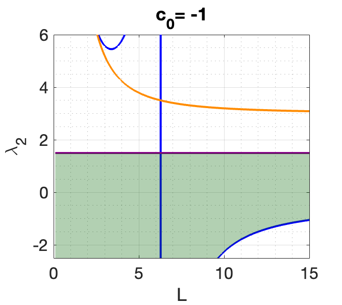
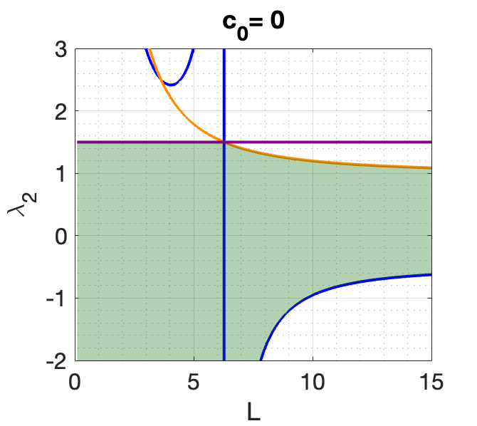
(c)	(d)
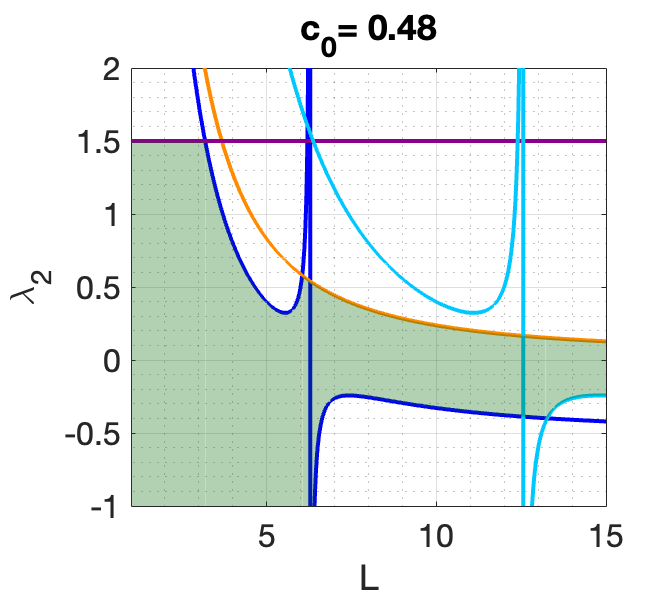
	30mm

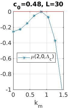
Figure 2: (a–c) Instability curves in the $L$–$\lambda_{2}$ plane ($\lambda_{1}$ according to (2)) for different values of $c_{0}$, delimiting the $\lambda_{2}$ parameter range for stability of ${\cal C}_{L}$. The blue curve correspond to the mode $(m,n)=(1,0)$ (minimal wave number pearling instability), the orange to $(m,n)=(1,1)$ (minimal wave number coiling/buckling) and the violet $\lambda_{2}=3/2$ to $(m,n)=(0,2)$ (wrinkling, independent of $L$). Lighter blue in (c) correspond to $(m,n)=(2,0)$, which gives the only finite wave number (independent of $L$) instability. (d) illustrates the long wave nature of the (1,0) pearling instability at $(c_{0},L)=(0,30)$ (as $k_{m}=0$ is forbidden by the area (or volume) constraint, and the finite wave number nature of the (2,0) pearling instability at $(c_{0},L)=(0.48,30)$.

Next we consider the modes $m\neq 0\neq n$, in particular $(m,n)=(1,1)$, where

$$\mu(1,1,\Lambda) =-\frac{1}{2}((k_{1}^{2}+1)^{2}+(\lambda_{2}+1)(k_{1}^{2}+1)-\left(\lambda_{2}+\frac{1}{2}\right)-(1-2c_{0})k_{1}^{2}$$

$$=-\frac{1}{2}(k_{1}^{2}+1)^{2}+(\lambda_{2}-2c_{0})k_{1}^{2}+\frac{1}{2}.$$

One sees directly that $\mu(1,1,\Lambda)$ is strictly increasing in $\lambda_{2}$ and has a zero for

$$\lambda_{2}^{(1,1)}=\frac{1}{2}k_{1}^{2}+1-2c_{0},$$ (47)

where $\lambda_{2}$ is strictly decreasing in $L$ because so is $k_{m}=2m\pi/L$. Hence, if $c_{0}>-1/4$, then there exists an $L$ large enough so that the cylinder destabilizes due to the $(m,n)=(1,1)$ mode with $L$ explicitly computable.

For $m\geq 1$ and $n=0$ (pearling), the eigenvalues

$$\mu(m,0,\Lambda)=-\frac{1}{2}k_{m}^{4}+(\lambda_{2}+2c_{0})k_{m}^{2}-\lambda_{2}-\frac{1}{2}$$

behave as follows. Depending on $L$, either $k_{m}<1$ such that $\mu(m,0,\Lambda)$ is strictly decreasing in $\lambda_{2}$, or $k_{m}>1$ such that $\mu(m,0,\Lambda)$ is strictly increasing in $\lambda_{2}$. In either case, for $m=1$ the eigenvalue has a zero at

$$\lambda_{2}^{(m,0)}=\Big{[}1-k_{m}^{2}\Big{]}^{-1}\Bigg{(}-\frac{1}{2}k_{m}^{4}+2c_{0}k_{m}^{2}-\frac{1}{2}\Bigg{)}$$ (48)

for all $L\in{\mathbb{R}}\backslash\{2\pi m\}$. First we note that the asymptote at $L=2\pi m$ is odd, where for $c_{0}<\frac{m}{2}$, $\lim_{k_{m}\searrow 1}\lambda_{2}=-\infty$ and for $c_{0}>\frac{m}{2}$ the other way around. In the latter case there always exists a $L$ such that the $m$’th mode destabilizes the cylinder, so we do not focus further on that case. A straightforward analysis of (48) shows that it admits two positive solutions

$$L=\begin{cases}L_{G}=2\pi\left(\frac{1+\sqrt{2}\sqrt{1-2c_{0}}}{4c_{0}-1}\right)^{1/2}\quad\text{ for }c_{0}\in(1/4,1/2],\\ L_{S_{1}}=2\pi\left(\frac{1-\sqrt{2}\sqrt{1-2c_{0}}}{4c_{0}-1}\right)\quad\text{ for }c_{0}\in(-\infty,1/2],\\ L_{S_{2}}=\sqrt{2}\pi,{\hskip 56.9055pt}\text{for }c_{0}=1/4,\end{cases}$$

where for $i=1,2$ it holds that $L_{S_{i}}<2\pi$ and are minima. For $c_{0}\leq\frac{1}{2}$ and $L>2\pi$ the eigenvalue $\mu(1,0,\Lambda)$ has negative slope at (48), hence for smaller $\lambda_{2}$ the cylinder is destabilized. In the case of $c_{0}\leq\frac{1}{4}$, $\lambda_{2}$ is monotonously increasing in $L$, yielding a maximum wavelength instability. In the regime where $L_{G}$ exists, the ${\cal C}_{L}$ destabilizes to a finite wave length.

In the following Corollary of Theorem 3.1 we summarize the above, where maximal wave length (or long wave instability) refers to the minimal allowed $k_{1}=2\pi/L$, since $k_{0}=0$ is prohibited by the volume and area constraints.

Corollary 3.2.

The cylinder ${\cal C}_{L}$ is volume and area preserving stable for every $L>0$ if:

1. $c_{0}\in(1/4,1/2)$ and $\lambda_{2}\in(\lambda_{2}^{(1,0)},\lambda_{2}^{(1,1)})$; ${\cal C}_{L}$ destabilizes at $\lambda_{2}^{(1,0)}$ with finite wave length $L_{G}$ wrt the mode $\psi_{20}$ (pearling), and at $\lambda_{2}^{(1,1)}$ wrt the mode $\psi_{11}$ (buckling and coiling) of maximal wave length.

2. $c_{0}\in[-1/4,1/4]$ and $\lambda_{2}\in(\lambda_{2}^{(1,0)},\lambda_{2}^{(1,1)})$; ${\cal C}_{L}$ destabilizes at $\lambda_{2}^{(1,0)}$ wrt to the mode $\psi_{10}$ (pearling), and at $\lambda_{2}^{(1,1)}$ wrt the mode $\psi_{11}$ (buckling and coiling), both of maximal wave length.

3. $c_{0}\in(-\infty,-1/4]$ and $\lambda_{2}\in(\lambda_{2}^{(1,0)},\lambda_{2}^{(0,2)})$; ${\cal C}_{L}$ destabilizes at $\lambda_{2}^{(1,0)}$ wrt the mode $\psi_{10}$ (pearling) with maximal wave length, and at $\lambda_{2}^{(0,2)}$ wrt the mode $\psi_{01}$ (wrinkling, homogeneous in $x$).

If $c_{0}>1/2$ there is always a positive eigenvalue for every $\lambda_{2}$, hence the cylinder is spectrally unstable.

4 Bifurcations from ${\cal C}_{L}$

We now compute the branches bifurcating at the instabilities given in Corollary 3.2. In §4.1 we give the general symmetry based bifurcation results, and in §4.2 we derive the associated amplitude equations and moreover discuss the stability of the bifurcating branches.

4.1 General bifurcation results

As a bifurcation problem, the desired primary bifurcation parameter is either ${\cal V}$ or ${\cal A}$. However, these parameters do not change along the trivial $u=0$ branch, and therefore we first choose $\lambda_{2}$ as the primary bifurcation parameter and only consider (42), which we write as

$$\eta(u){\partial}_{t}u =G(u,\Lambda),$$ (49a)

$$0 ={\cal A}(u)-{\cal A}_{0}.$$ (49b)

The linearization of (49) is the first $2\times 2$ block of ${\partial}_{U}{\cal G}$, hence with eigenvalues (39) with $(m,n)\in{\mathbb{Z}}^{2}\backslash\{(0,0),(0,\pm 1)\}$, and eigenvectors

$$\Psi_{mn}(x,\varphi)=\begin{pmatrix}A_{mn}e^{{\rm i}(k_{m}x+n\varphi)}+\mathrm{c.c.}\\ 0\end{pmatrix}.$$ (50)

Here $\mu_{00}$ is not present since it corresponds to changes of radius along the cylinder branch. Solving (2) gives (possible) bifurcation points (for completeness with $r$–dependence)

$$\lambda_{2}=\Bigg{[}\frac{(1-n^{2})}{r^{2}}-k_{m}^{2}\Bigg{]}^{-1}\bigg{(}-\frac{1}{2}\Big{[}k_{m}^{2}+\frac{n^{2}}{r^{2}}\Big{]}^{2}+\frac{1}{r^{2}}\Big{[}k_{m}^{2}+\frac{n^{2}}{r^{2}}\Big{]}-\left(\frac{1}{r}-2c_{0}\right)\frac{k_{m}^{2}}{r}-\frac{1}{2r^{4}}\bigg{)}.$$ (51)

Due to symmetries the bifurcation points have multiplicities at least two, and hence the equivariant branching lemma [CL00, GS02, Hoy06] gives the needed framework for the bifurcation analysis.

Theorem 4.1.

At (51) in the system (49) we have equivariant pitchfork bifurcations of steady state solutions $X(\varepsilon)=\mathcal{C}_{r}(L)-u(\varepsilon)N$, $\Lambda(\varepsilon)=\Lambda_{0}+{\cal O}(\varepsilon^{2})$, for some $0<|\varepsilon|<\varepsilon_{0}$ sufficiently small. The maps $\varepsilon\mapsto(u(\varepsilon),\Lambda(\varepsilon))\in H^{4}\times{\mathbb{R}}^{2}$, or, equivalently $\varepsilon\mapsto(X(\varepsilon),\Lambda(\varepsilon))\in H^{4}_{\text{per}}(\mathcal{C}_{r}(L),{\mathbb{R}}^{3})\times{\mathbb{R}}^{2}$ are analytic, and we characterize the bifurcations as follows:

1. $n=0$ (pearling):

   $$u=\left(A_{m}e^{{\rm i}k_{m}x}+\mathrm{c.c.}\right)\varepsilon+{\cal O}(\varepsilon^{2})$$ (52)

   with some amplitude $A_{m}\in{\mathbb{C}}$, equivariant wrt translations in $x$.

2. $m=0$ (wrinkling):

   $$u=\left(A_{n}e^{{\rm i}n\varphi}+\mathrm{c.c.}\right)\varepsilon+{\cal O}(\varepsilon^{2})$$ (53)

   with some amplitude $A_{n}\in{\mathbb{C}}$, equivariant wrt rotations in $\varphi$.

3. $m\neq 0\neq n$ (buckling and coils): Two types branches bifurcate. Buckling

   $$u=\left(A_{mn}e^{{\rm i}(k_{m}x+n\varphi)}+\mathrm{c.c.}\right)\varepsilon+{\cal O}(\varepsilon^{2}),$$ (54)

   equivariant wrt to translations in $x$ and rotations in $\phi$. The other branch are coils as equal amplitude superpositions of buckling,

   $$u=\left(A_{mn}e^{{\rm i}(k_{m}x+n\varphi)}+A_{m-n}e^{{\rm i}(k_{m}x-n\varphi)}+\mathrm{c.c.}\right)\varepsilon+{\cal O}(\varepsilon^{2}),$$ (55)

   equivariant wrt to translations in $x$, or, equivalently wrt rotations in $\phi$, which yield the same group orbit.

Proof.

The proof proceeds via the equivariant branching lemma, see for example [CL00, Theorem 2.3.2]. By Equation 29, $B(u)$ is elliptic, hence the linearization of $G(u,\Lambda)$ is elliptic as well, and hence the upper left $2\times 2$ block of ${\partial}_{U}{\cal G}$ is a Fredholm operator. At every $\lambda_{2}$ from (51), the zero eigenvalue is of finite multiplicity, namely multiplicity 2 in (a,b), and multiplicity 4 in (c), and the symmetries of the bifurcating branches are as follows:

1. $X(\varepsilon)$ admits a new non trivial symmetry wrt translations in $x$. Assume that $A_{-m}=A_{m}$ with $A_{m}\in{\mathbb{R}}$, so that $u=\cos(k_{m}x)$. The (not normalized) normal vector is

   $$\nu={\partial}_{x}X(\varepsilon)\times{\partial}_{\varphi}X(\varepsilon) =\begin{pmatrix}1\\ -k_{m}\sin(k_{m}x)\cos(\varphi)\\ -k_{m}\sin(k_{m}x)\sin(\varphi)\end{pmatrix}\times\begin{pmatrix}0\\ -(1+\cos(k_{m}x))\sin(\varphi)\\ (1+\cos(k_{m}x))\sin(\varphi)\end{pmatrix}$$

   $$=-(1+\cos(k_{m}x))\begin{pmatrix}k_{m}\sin(k_{m}x)\\ \cos(\varphi)\\ \sin(\varphi)\end{pmatrix}.$$

   Hence $\left\langle\nu,e_{j}\right\rangle\neq 0$ for $j=1,2,3$, hence $\rm{span}\{\left\langle\nu,e_{j}\right\rangle\}$ is a subset of the generator of the center manifold of $X(\varepsilon)$. Following this with

   $$X(\varepsilon)\times e_{1}=\begin{pmatrix}0\\ -(1+\cos(x))\sin(\varphi)\\ (1+\cos(x))\cos(\varphi)\end{pmatrix},$$

   we have that $\left\langle X(\varepsilon)\times e_{1},\nu\right\rangle=0$.

2. As for (a) we can calculate the center manifold in the bifurcating branch, with

   $$\nu={\partial}_{x}X(\varepsilon)\times{\partial}_{\varphi}X(\varepsilon)=\begin{pmatrix}0\\ 2\sin(2\varphi)\sin(\varphi)+\cos(2\varphi)\cos(\varphi)\\ 2\sin(2\varphi)\cos(\varphi)+\cos(2\varphi)\sin(\varphi)\end{pmatrix}$$

   and

   $$\left\langle X(\varepsilon)\times e_{1},\nu\right\rangle=\left\langle\begin{pmatrix}0\\ (1+\cos(2\varphi))\sin(\varphi)\\ -(1+\cos(2\varphi))\cos(\varphi)\end{pmatrix},\nu\right\rangle=\cos(2\varphi)(1+\cos(2\varphi))\cos(\varphi)\sin(\varphi).$$

   Hence in the center manifold of $X(\varepsilon)$ are besides the translation in $y$ and $z$ direction also rotations around the $x$ axis.

3. The 4D kernel generates two different types of branches. For the coils we have

   $${\partial}_{x}X(\varepsilon) =\begin{pmatrix}1\\ 0\\ 0\end{pmatrix}-k_{m}\sin(k_{m}x+n\varphi)\begin{pmatrix}0\\ \cos(\varphi)\\ \sin(\varphi)\end{pmatrix}$$

   $${\partial}_{\varphi}X(\varepsilon) =(1+\cos(k_{m}x+n\varphi)\begin{pmatrix}0\\ -\sin(\varphi)\\ \cos(\varphi)\end{pmatrix}-n\sin(k_{m}x+n\varphi)\begin{pmatrix}0\\ \cos(\varphi)\\ \sin(\varphi)\end{pmatrix}$$

   so the normal vector is

   $$\nu= (1+\cos(k_{m}x+n\varphi)\begin{pmatrix}0\\ -\cos(\varphi)\\ -\sin(\varphi)\end{pmatrix}-n\sin(k_{m}x+n\varphi)\begin{pmatrix}0\\ -\sin(\varphi)\\ \cos(\varphi)\end{pmatrix}$$

   $$-k_{m}\sin(k_{m}x+n\varphi)(1+\cos(k_{m}x+n\varphi))\begin{pmatrix}1\\ 0\\ 0\end{pmatrix}$$

   Obviously, this results in a non trivial translational symmetry in $x$. Similarly

   $$X(\varepsilon)\times e_{1}=\begin{pmatrix}0\\ -(1+\cos(k_{m}x+n\varphi))\sin(\varphi)\\ (1+\cos(k_{m}x+n\varphi))\cos(\varphi)\end{pmatrix},$$

   such that $\left\langle X(\varepsilon)\times e_{1},\nu\right\rangle=n\sin(k_{m}x+n\varphi)(1+\cos(k_{m}x+n\varphi))$ yields the same action as the translation. For the buckling solutions similar computations show that $\mathrm{span}\{\left\langle\nu,e_{1}\right\rangle,\left\langle X(\varepsilon)\times e_{1},\nu\right\rangle\}$ is two dimensional, hence the full symmetry is needed.

∎

4.2 Reduced equation

To further describe the bifurcations from Theorem 4.1, we derive the reduced equations (or amplitude equations AEs) at ${\cal C}_{L}$. These are straight forward computations, but somewhat cumbersome in our geometric setting and thus we partly use Maple. Here we explain the basic steps, and the computations for the pearling and wrinkling instability, but for the coils vs buckling we relegate some details to Appendix LABEL:aeapp. Additionally we give the numerical values of the coefficients of the AEs for some of examples, which will later be compared to numerics for the full problem.

According to Theorem 4.1, at “simple” (strictly speaking of multiplicity two, but from here we factor out the translation or rotation) bifurcation points (51), i.e., $(m,n)=(m,0)$ or $(m,n)=(0,n)$, the bifurcating steady state branch is tangential to solutions of $D{\cal G}(0,\Lambda)[(\psi,0)]=0$ where ${\cal G}$ is the rhs of (49). We thus introduce the small parameter

$$\varepsilon=\sqrt{\left|\frac{\lambda_{2}-\lambda_{2}(m,n)}{\beta_{2}}\right|},$$ (56)

where $\beta_{2}=\pm 1$ is introduced for later convenience to deal with sub–and supercritical pitchforks, and altogether we use the ansatz

$$u=\varepsilon A\psi_{m,n}+\varepsilon^{2}\sum_{(i,j)\in{\cal B}}A_{i,j}\psi_{i,j}+\mathrm{c.c.}+{\cal O}(\varepsilon^{3}),$$ (57)

$$\lambda_{2}=\lambda_{2}(m,n)+\beta_{2}\varepsilon^{2}+{\cal O}(\varepsilon^{3}),\quad\lambda_{1}=\lambda_{1}(m,n)+\alpha_{2}\varepsilon^{2}+{\cal O}(\varepsilon^{3}),\quad$$ (58)

where ${\cal B}$ is the index set of the modes generated from the critical modes in quadratic interactions, $A=A(T)$, $A_{i,j}=A_{i,j}(T)$, and $T=\varepsilon^{2}t$. The $O(2)\times O(2)$ symmetry of the system (translations and reflections in $x$, and in $\varphi$, where for the simple bifurcations only one is nontrivial, translation for pearling, and rotation for wrinkles) is inherited by the reduced equation which hence has the form $\ddT A=Ag(A,\overline{A},(\alpha_{j})_{j=1,\dots,N-1},(\beta_{j})_{j=1,\dots,N-1}),$ where $g$ is an even function in all variables, i.e., in lowest order

$$\ddT A=A\left(a\beta_{2}+b|A|^{2}\right).$$ (59)

At the “double” BPs $m\neq 0\neq n$ two types of branches bifurcate, and we give the ansatz below.

Near a bifurcation point from a stable branch, the critical mode determines the evolution, while all others are exponentially damped. Hence, in a standard AE setting, the signs of $a$, $\beta_{2}$ and $b$ in (59) determine the stability on the bifurcating branch. Here, from (59) we get stability information for steady states under area constraint, with $\lambda_{2}$ as extrinsic fixed parameter, but this can be extended to stability under area and volume constraints as follows. Close to the bifurcation point $\lambda_{2}(m,n)$ the solution reads $X(\varepsilon)={\cal C}_{L}-\varepsilon A\psi N$. Then the solution is linearly stable iff ${\partial}_{U}{\cal G}(X(\varepsilon),\Lambda)$ (which includes the $q_{1}$ area constraint) has only negative eigenvalues. For admissible (area and volume preserving) perturbations $\phi:{\cal C}_{L}\rightarrow{\mathbb{R}}$ of $X(\varepsilon)$, we have the necessary and sufficient conditions

$$\int_{X(\varepsilon)}H(\varepsilon A\psi)\phi\,{\rm d}S=\int_{X(\varepsilon)}\varepsilon A\psi g^{-1/2}(\varepsilon A\psi)\phi\,{\rm d}S=0.$$

For the mean curvature we have $H(\varepsilon A\psi)=\frac{1}{2}-\varepsilon A(\mu(m,n)+1)\psi+{\cal O}(\varepsilon^{2})$, and hence admissible perturbations must be orthogonal to $\psi$. Thus, near bifurcation points associated with loss of stability of ${\cal C}_{L}$ we have the following results:

• Branches bifurcating from simple bifurcation points (pearling or wrinkling), are stable wrt (7).

• Solutions on branches from a double bifurcation point (buckling and coiling), can only be destabilized by the other kernel vectors. We will see examples of this in §5.

4.2.1 Pearling instability

For the pearling instability (with for notational simplicity $m=1$) we have

$$\varepsilon\,u=\varepsilon A\,\psi_{10}+\varepsilon^{2}\left(\frac{1}{2}A_{0}\psi_{00}+A_{2}\,\psi_{20}\right)+\mathrm{c.c.}+{\cal O}(\varepsilon^{3}),\quad\varepsilon=\sqrt{\left|\frac{\lambda_{2}(1,0)-\lambda_{2}}{\beta_{2}}\right|},$$

with $A=A(T),\ T=\varepsilon^{2}t$. Plugging into (49) and sorting by powers of $\varepsilon$, with the abbreviations $\lambda_{2}=\lambda_{2}(1,0)$ and $k=k_{1}$, we obtain the following:

• $\displaystyle 0=-\frac{1}{2}\left(\left(k^{4}+\left(-4c_{0}-2\lambda_{2}\right)k^{2}+2\lambda_{2}+1\right)\right)A.$

• $\displaystyle 0=\left(-\lambda_{2}-\frac{1}{2}\right)A_{0}+\frac{1}{2}\left(\left(k^{4}+\left(-8c_{0}-2\lambda_{2}-1\right)k^{2}+4\lambda_{2}+5\right){|A|}^{2}\right)-\beta_{2}-\alpha_{2}.$

• $\displaystyle 0=\left(-\frac{7k^{4}}{4}{+}\frac{\left(-3-8c_{0}+2\lambda_{2}\right)k^{2}}{4}{+}\lambda_{2}{+}\frac{5}{4}\right)A^{2}+\left(-8k^{4}{+}\frac{\left(32c_{0}{+}16\lambda_{2}\right)k^{2}}{4}{-}\lambda_{2}{-}\frac{1}{2}\right)A_{2}$.

• $${\hskip-11.38109pt}\ddT A= \left(\frac{5k^{6}}{2}{+}\frac{\left(1{-}8c_{0}{-}3\lambda_{2}\right)k^{4}}{2}{+}\frac{\left(\frac{7}{2}{+}12c_{0}{+}\lambda_{2}\right)k^{2}}{2}{-}\frac{27}{4}{-}3\lambda_{2}\right)A{|A|}^{2}{+}\left(\frac{\left({-}4c_{0}{-}1\right)k^{2}}{2}{+}2\lambda_{2}{+}\frac{5}{2}\right)AA_{0}$$

  $${+}\left(4k^{4}{+}4\left({-}\frac{3}{8}{-}\frac{5c_{0}}{2}{-}\frac{\lambda_{2}}{2}\right)k^{2}{+}4\left(\frac{5}{8}{+}\frac{\lambda_{2}}{2}\right)\right)\overline{A}A_{2}+\left(-k^{2}+1\right)\alpha_{2}A.$$

From the area constraint we get the condition $0=A_{0}+k^{2}|A|^{2}$ for the $\psi_{00}$ mode, which gives

$$\alpha_{2}=\frac{1}{2}\left(k^{4}-8k^{2}c_{0}+4\lambda_{2}+5\right){|A|}^{2}-\beta_{2}.$$

We used directly the $\varepsilon$ scale of $\lambda_{2}$, hence we only get back the zero eigenvalue at $\varepsilon\psi_{1}$. The above equations at $\varepsilon^{2}\psi_{00}$ and $\varepsilon^{2}\psi_{20}$ give

$$A_{0} =\frac{1}{2\lambda_{2}+1}\left(\left(k^{4}+\left(-8c_{0}-2\lambda_{2}-1\right)k^{2}+4\lambda_{2}+5\right){|A|}^{2}+-2\alpha_{2}-2\beta_{2}\right),\text{ and}$$ (60)

$$A_{2} =-\frac{A^{2}\left(7k^{4}+\left(3+8c_{0}-2\lambda_{2}\right)k^{2}-4\lambda_{2}-5\right)}{2\left(16k^{4}+\left(-16c_{0}-8\lambda_{2}\right)k^{2}+2\lambda_{2}+1\right).}$$ (61)

The dependence on $\beta_{2}$ here comes from the dependence of $\lambda_{1}$ on $\lambda_{2}$. Combining everything leads at $\varepsilon^{3}\psi_{10}$ to the solvability condition (59) with

$$a= k^{2}-1,$$

$$b= \frac{5}{\left(k^{2}{-}1\right)k^{2}\left(4k^{4}{-}5k^{2}{+}4c_{0}{-}1\right)}\Bigg{(}\frac{3}{20}{+}k^{14}{+}\left(4c_{0}{-}\frac{73}{20}\right)k^{12}{+}\left(\frac{8c_{0}}{5}{-}\frac{13}{10}\right)k^{10}{+}\left(\frac{32}{5}c_{0}^{2}{-}\frac{52}{5}c_{0}{+}\frac{73}{20}\right)k^{8}$$

$${+}\left(\frac{16}{5}c_{0}^{2}{-}8c_{0}{+}\frac{31}{5}\right)k^{6}{+}\left(\frac{4c_{0}}{5}{-}\frac{43}{20}\right)k^{4}{+}\left(\frac{12c_{0}}{5}{-}\frac{3}{2}\right)k^{2}\Bigg{)}.$$

Recall that here $k=k_{m}=2m\pi/L$, hence $a<0$ for $L>2m\pi$, and similarly $b<0$ for non small $L$. For instance, $a\approx-0.6$ and $b\approx-3$ in Fig.5, where we compare the AE predictions for $m=1$ pearling with $c_{0}=0$ and $L=10$ with numerics. In any case for $ab>0$ we set $\beta_{2}=-1$ (subcritical case), and otherwise $\beta_{2}=1$ (supercritical case), giving the amplitude $A=\sqrt{\left|\frac{a}{b}\right|}$, with also $\alpha_{2}$ uniquely determined. The change of the volume can be approximated by inserting the amplitude Ansatz, giving $0=A_{0}+A^{2}+\beta_{2}$ at $\varepsilon^{2}\psi_{00}$, and comparison with (60) shows that preserving the area and the volume is not possible along the pearling branch.

4.2.2 Wrinkling instability

For the primary wrinkling instability at $\lambda_{2}(0,2)=3/2$ we have the ansatz

$$\varepsilon\,u(\varphi)=\varepsilon Ae^{2{\rm i}\varphi}+\varepsilon^{2}\left(\frac{1}{2}A_{0}+A_{4}e^{4{\rm i}\varphi}\right)+\mathrm{c.c.}+{\cal O}(\varepsilon^{3}),$$

again with $\varepsilon=\sqrt{\frac{|\lambda_{2}-\lambda_{2}^{(0,2)}|}{\beta_{2}}}$ and $A=A(T)$, $T=\varepsilon^{2}t$, and obtain the following.

• $\displaystyle 0=3A\left(\lambda_{2}-\frac{3}{2}\right)$.

• $\displaystyle 0=\frac{1}{4}\left(-40\lambda_{2}+82\right){|A|}^{2}-\left(\lambda_{2}+\frac{1}{2}\right)A_{0}-\beta_{2}-\alpha_{2}$.

• $\displaystyle 0=\left(-9\lambda_{2}+\frac{369}{4}\right)A^{2}+\left(15\lambda_{2}-\frac{225}{2}\right)A_{4}$.

• $\displaystyle\ddT A=-6\left(\lambda_{2}-\frac{11}{4}\right)AA_{0}+\frac{1}{4}\left(-120\lambda_{2}+1170\right)\overline{A}A_{4}-3A\alpha_{2}-3\left(-\lambda_{2}+\frac{221}{4}\right){|A|}^{2}A$.

From the area constraint at $\varepsilon^{2}\psi_{00}$ we have $0=8|A|^{2}+2A_{0}$, leading to $\alpha_{2}=\frac{3\left(15-4\lambda_{2}\right){|A|}^{2}}{2}-\beta_{2}$. Thus $\lambda^{(0,2)}_{2}=\frac{3}{2}$, $A_{0}=\frac{11}{4}|A|^{2}-\frac{\beta_{2}}{2}-\frac{\alpha_{2}}{2}$, $A_{4}=\frac{7}{8}A^{2}$ and finally $\alpha_{2}=\frac{27}{2}|A|^{2}-\beta_{2}$. This ultimately leads to the solvability condition

$$\ddT A=(3\beta_{2}-15.19|A|^{2})A,$$ (62)

which is notably independent of $c_{0}$ and $L$, and yields supercritical wrinkling bifurcations for $\beta_{2}=1$.

4.2.3 Coiling/buckling instability

For the instability with critical wave vector $(m,n)=(1,1)$ and $(m,n)=(1,-1)$ we choose the ansatz

$$\varepsilon\,u(x,\varphi)=\varepsilon\left(A\psi_{11}+B\psi_{1-1}\right)+\varepsilon^{2}\left(\frac{1}{2}A_{00}+A_{22}\psi_{22}+B_{22}\psi_{2-2}+A_{20}\psi_{20}+A_{02}\psi_{02}\right)+\mathrm{c.c.}+{\cal O}(\varepsilon^{3}),$$ (63)

with $\varepsilon=\sqrt{\frac{|\lambda_{2}-\lambda_{2}^{mm}|}{\beta_{2}}}$ and $T=\varepsilon^{2}t$. Using the amplitude formalism, this gives a cubic system of reduced equations for $A,B$, which by $O(2)\times O(2)$ symmetry must read

$$\ddT A =A(a\beta_{2}+b_{1}|A|^{2}+b_{2}|B|^{2}),$$ (64a)

$$\ddT B =B(a\beta_{2}+b_{2}|A|^{2}+b_{1}|B|^{2}).$$ (64b)

From that we can directly recover the two types of solutions: Buckling with $\displaystyle A=\sqrt{\left|\frac{a}{b_{1}}\right|}$ and $B=0$ or the other way round; coiling with $\displaystyle A=B=\pm\sqrt{\left|\frac{a}{b_{1}+b_{2}}\right|}$. Here again $\beta_{2}=\pm 1$, depending on the signs of $a$, $b_{1}$, and $b_{1}+b_{2}$.

We have $a=k_{m}^{2}$, but the computation of the coefficients $b_{1}$ and $b_{2}$ naturally is more cumbersome than for the scalar case (pearling and wrinkling), and therefore relegated to Appendix LABEL:aeapp. Here we instead briefly comment on the bifurcation directions, and stability of the bifurcating branches under volume and area preserving flows, see also Fig.3. The Jacobian of the rhs of (64) at a steady state $(A,B)$ is

$$\begin{pmatrix}a+3b_{1}A^{2}+b_{2}B^{2}&2b_{2}AB\\ 2b_{2}AB&a+b_{2}A^{2}+3b_{1}B^{2}\end{pmatrix}.$$

For $a>0$, on the coil solution branch the eigenvalues are $\sigma_{1}=(a\beta_{2}+3{\rm sign}(b_{1})|a\beta_{2}|)$ and $\sigma_{2}=(a\beta_{2}+\frac{b_{2}}{|b_{1}|}|a\beta_{2}|)$. Hence the coils are stable for $\frac{b_{2}}{|b_{1}|}<-{\rm sign}(\beta_{2})$.

For the buckling the Jacobian has the eigenvalues

$$\sigma_{1}=2\frac{b_{2}+b_{1}}{|b_{1}+b_{2}|}\quad\sigma_{2}=\frac{b_{2}-b_{1}}{|b_{1}+b_{2}|},$$

where $\sigma_{1}$ corresponds to the eigenvector $v_{1}=(1,1)^{T}$ and $\sigma_{2}$ to $v_{2}=(1,-1)^{T}$. Hence the relevant eigenvalue is $\sigma_{2}$, which is negative for $b_{2}<b_{1}$. In §5 we give two comparisons of the predictions from (64) with numerics, namely $c_{0}$ and $L=10$ yielding $(a,b_{1},b_{2})\approx(0.39,-0.67,-0.82)$ in Fig.4, and $c_{0}=0.48$ and $L=10$ yielding $(a,b_{1},b_{2})=(0.39,-0.083,0.56)$ in Fig.9. In both cases we get the correct branching and stability predictions, and also very good quantitative agreement.

Figure 3: Schematic linearized stability diagram of the amplitude equation depending on $b_{1}$ and $b_{2}$ . Orange stands for the coil and green for the wave branch. Thick lines indicate stable solutions.

5 Numerical examples

We now use numerical continuation and bifurcation methods to corroborate the local results from §4, and to extend them to a more global picture. This includes the study of secondary bifurcations with interesting stable shapes far away from the cylinder. The numerical setup follows the stability analysis in subsection 3.3 and §4.2. Namely, we throughout fix the period $L$, and the area ${\cal A}={\cal A}(X)$, and initially use $\lambda_{2}$ as the primary bifurcation parameter and $\lambda_{1}$ and ${\cal V}(X)$ as secondary (dependent) parameters. The linearized stability of the solutions, however, is then computed for fixed ${\cal A}(X)$ and ${\cal V}(X)$ while $\lambda_{1}$ and $\lambda_{2}$ are free parameters. Due to the radius-length scaling invariance of the Helfrich energy (3) and the area and volume constraint in the dynamical problem, it is useful to introduce the reduced volume

$$v={\cal V}(X)/{\cal V}_{0},$$ (65)

where ${\cal V}_{0}$ is the volume of the straight cylinder with the same ${\cal A}(X)$, compare [JSR93], and we normalize the energy

$$\tilde{E}(X)=\frac{1}{{\cal A}}\int_{X}(H-c_{0})^{2}\,{\rm d}S.$$ (66)

Also for our numerics we focus on the three exemplary cases

(a) $$c_{0}=0 c_{0}=-1 c_{0}=0.48$$, (b) ,  and (c)

from Fig.2, and mostly we use $L=10$. For (a) and (b) this is no significant restriction as in these cases the primary bifurcations (to pearling, buckling and coiling in (a), and to pearling and wrinkling in (b)) are of long wave type for any (sufficiently large) $L$, i.e., a different $L$ gives the same types of primary bifurcations with different axial (maximal) periods $L$ (and the wrinkling is independent of $L$). However, for (c) and sufficiently large $L$ (preferably an integer multiple of the critical period $\ell\approx 7.5$) we have a finite wave number pearling instability. Thus, besides the case $L{=}10$ (for comparison with (a) and (b)), for (c) we shall consider different multiples of 7.5 for $L$, namely $L{=}15,L{=}30$, and $L{=}45$, allowing 2, 4, and 6, pearls on the primary branch. The influence of $L$ will then be the behavior of this branch away from bifurcation, which loses stability in a bifurcation to a single pearl branch, and this BP moves closer to the primary BP with increasing $L$. This is further discussed in §LABEL:dsec.

In the numerics we (as always) have to find a compromise between speed and accuracy. For the default $L=10$ we start with an initial discretization of the straight cylinder ${\cal C}_{L}$ by $n_{p}\approx 3000$ mesh points; the continuation of the nontrivial branches then often requires mesh refinement (and coarsening), typically leading to meshes of 4000 to 5000 points. For the longer cylinders for $c_{0}=0.48$ we increase this to up to 12000 mesh points. A simple measure of numerical resolution is the comparison of the $\lambda_{2}$ values of the numerical BPs from ${\cal C}_{L}$ with their analytical values from §3.1, and here we note that in all cases we have agreement of at least 4 digits. Moreover, we also compare some numerical nontrivial branches with their descriptions by the AEs, and find excellent agreement.

Remark .

Some cylindrical solutions have similarities with axisymmetric closed vesicle solutions of (LABEL:helf0). We recall from [JSR93] or [MU24], that from the sphere the first bifurcation is to prolates (rods) and oblates (wafers). For mildly negative or positive $c_{0}$ the prolates are stable near bifurcation and the oblates unstable, and continuing the prolates they become dumbbells (two balls connected by a thin neck), from which pea shaped vesicles bifurcate which become stable as one of the ball shrinks. For sufficiently negative $c_{0}$, the oblates are stable near bifurcation, and continuing the branch they become discocytes of biconcave red blood cell shape. Here we see some reminiscent behavior, e.g., secondary bifurcations of stable wrinkles with “embedded biconcave shapes” for sufficiently negative $c_{0}$, see, e.g., Fig.7E, and secondary bifurcations to “unequal pearls” from the pearling at positive $c_{0}$ (see Figures 10–12). $\rfloor$

We complement our results by some (area and volume conserving) numerical flows close to steady states, and for these perturb steady states $X_{0}$ in two different ways: one is

$$\tilde{X}_{0}=X_{0}+\delta u_{0}N_{0},\quad u_{0}=\frac{1}{1+\xi x^{2}}\cos(\varphi),$$ (67)

where $x$ is the coordinate along the cylinder axis, and $\varphi$ the polar angle orthogonal to it, and $\delta\in{\mathbb{R}}$ and $\xi>0$ are parameters, with typically $\xi=1$ and $\delta=-0.125$ or $\delta=-0.25$ (recall that $N$ is the inner normal). The other way is

$$\tilde{X}_{0}=X_{0}+\delta u_{0}N_{0},\quad\quad\text{with $u_{0}=\psi_{\text{crit}}$},$$ (68)

where $\psi_{\text{crit}}$ is (the $u$ component of) the eigenvector to the largest eigenvalue of the Jacobian at $X_{0}$, and typically $\delta=-0.5$. Due to the negative $\delta$ combined with the inner normal $N$, perturbations of type (67) in general induce a small increase of the initial volume ${\cal V}_{0}={\cal V}+{\cal V}_{\delta}$ and area ${\cal A}_{0}={\cal A}+{\cal A}_{\delta}$, which are conserved under the flow. On the other hand, perturbations of type (68) are area and volume preserving to linear order.

Our numerical flows $t\mapsto(X(t),\Lambda(t))=\Psinum(t;h)X_{0}$ are ad hoc approximations with a time stepsize $h$ and tolerance tol (see Appendix A.1), and we summarize the results from our flow experiments as follows:

1. Linearly stable $X_{0}$ (at $({\cal V},{\cal A})$) are also stable under the flow at the perturbed $({\cal V}_{0},{\cal A}_{0})$, and the solution flows back to the respective type (pearling, coiling, …) at $({\cal V}_{0},{\cal A}_{0})$, with a small change in $(\lambda_{1},\lambda_{2})$. See, e.g., Fig.6(a,b).

2. If $X_{0}$ at $({\cal V},{\cal A})$ is linearly unstable, then we generally expect $X(t)$ to flow to the nearest stable steady state (of in general a different class), see Fig.6(c₂). However, if we have a significant perturbation of $({\cal A}_{0},{\cal V}_{0})$, then $X(t)$ may still flow to a similar steady state close to $X_{0}$ by adapting $(\lambda_{1},\lambda_{2})$, see, e.g., Fig.6($c_{1}$). This underlines the fact that $\lambda_{1,2}$ are dynamical variables.

3. Naturally, we want $E$ to decrease monotonously in $t$, cf.(LABEL:helf1b), which if violated gives an easy indicator of poor numerics. The monotonous decrease of $E$ often requires rather small stepsizes and tolerances, and a result is that in many examples a single numerical flow to steady state is as expensive as the computation of the full BD of steady states, which we take as a strong argument for our steady state continuation and bifurcation approach.

5.1 $c_{0}=0$

For $L=10$ and $c_{0}=0$, Corollary 3.2 gives that the cylinder destabilizes at $\lambda_{2}\approx-0.95$ to pearling, $(m,n)=(1,0)$, and at $\lambda_{2}\approx 1.19$ to modes $(m,n)=(1,1)$. Figure 4 shows the BDs and samples starting in (a₁) with the energy $E$ over the reduced volume $v$.

(a1) (a2)

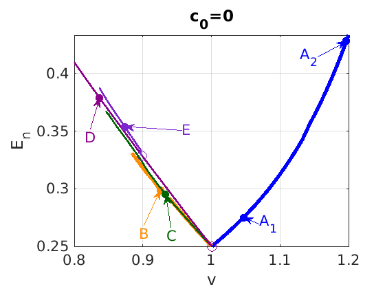
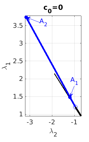
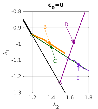
(b)

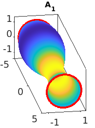
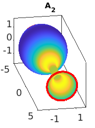
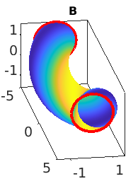
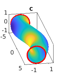
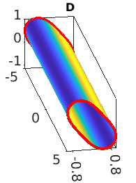
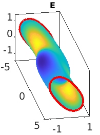
Figure 4: Basic BD for $c_{0}=0$, $L=10$. (a₁) Energy $E$ over reduced volume $v$. The family of cylinders $\mathcal{C}_{10}$ parameterized by $\lambda_{1}$ corresponds to the point where all primary branches bifurcate; A=pearls, B=coils, C=buckling, D=wrinkling; E is a secondary bifurcation from D, yielding a mix of buckling and wrinkling. (a₂) Relations between $\lambda_{1}$ and $\lambda_{2}$. The cylinders are the black branch, stable for $\lambda_{2}\in(-0.95,1.19)$. Bifurcation of A at $\lambda_{2}\approx-0.95$, bifurcation of B,C at $\lambda_{2}\approx 1.19$, and bifurcation of D at $\lambda_{2}=3/2$. Samples in (b); here the colors indicate $u$ from the current continuation step, with blue for $u<0$ (yellow for $u>0$) indicating that $X$ moves outward (inward) along the branch. The periodic boundaries are shown in red for better visibility.

Here all branches bifurcate from $v=1$, but (a₂) shows that they are well separated in the $(\lambda_{1},\lambda_{2})$ plane. As stated in subsubsection 4.2.1, the blue pearling branch starts stable close to the bifurcation point (sample A₁), and stays stable up to rather strong deformations of the original cylinder, sample A₂. The area constraint prevents the branch from growing to arbitrary volumes, but due to neck development the continuation becomes more difficult for larger $v$. From the mode $(m,n)=(1,1)$ at $\lambda_{2}\approx 1.19$ we find buckling and coiling. The coefficients in (64) are $(a,b_{1},b_{2})=(0.39,-0.4,-0.67)$, and as predicted (see Remark 5.1) the coiling (sample B) is stable close to bifurcation, while the buckling (sample C) is unstable. This behavior continues to small $v$, with no secondary bifurcations.

Additionally we show one wrinkling branch (sample D) as a later bifurcation from the cylinder, and a secondary bifurcation to a wrinkling–buckling mix (sample E). However, these solutions are all linearly unstable in the $\lambda_{1,2}$ range shown, at the given ${\cal V}$ and ${\cal A}$.

(a)
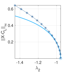
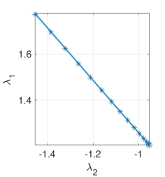
(b)

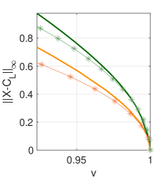
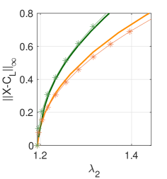
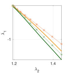
Figure 5: $c_{0}=0$, comparison of numerics and AE predictions (lines with *), (a) pearling, (b) coils (orange) and buckling (green). Left and center: Amplitude over reduced volume $v$, and over $\lambda_{2}$. Right: $\lambda_{1}$ over $\lambda_{2})$.

Remark .

The amplitude formalism in subsection 4.2 is only expected to be valid in a small neighborhood of the bifurcation points. In Fig. 5 we show comparisons between the numerical computations and the AE predictions. Here the amplitude formalism for the pearling

$$u=\varepsilon A\psi_{10}+{\cal O}(\varepsilon^{2}) \lambda_{2}=\lambda_{2}(1,0)-\varepsilon^{2} \lambda_{1}=\lambda_{1}(1,0)+\alpha_{2}\varepsilon^{2}+{\cal O}(\varepsilon^{4})$$, ,  ,

yields $\displaystyle\ddT A=A(0.61-2.96A^{2})$ and $\alpha_{2}=0.66A^{2}-1$, and that for the wrinkling $u=\varepsilon A\psi_{01}+{\cal O}(\varepsilon^{2})$, $\lambda_{2}=\lambda_{2}(0,1)+\varepsilon^{2}$, $\lambda_{1}=\lambda_{1}(0,1){+}\alpha_{2}\varepsilon^{2}{+}{\cal O}(\varepsilon^{4})$ yields the universal AE (62), i.e., $\displaystyle\ddT A=A(3{-}15.19A^{2})$ and $\alpha_{2}=\frac{27}{2}A^{2}{-}1$. For both, pearling and wrinkling, we find an excellent match with the numerics. $\rfloor$

In Fig.6 we show numerical flows from the steady states A–C from Fig.4, perturbed according to (67), with parameters given in Table 1. In all cases we integrate until $\|{\partial}_{t}u\|_{\infty}<0.001$. The plots on the left show the initially perturbed $X_{0}$, and $X$ at the end of the DNS colored by the last update $\delta u$, such that $u_{t}\approx\delta u/h$, where $h$ is the current stepsize. The plots on the right show the evolution of $E(t)$ and $\lambda_{1,2}$, and the relative errors in ${\cal A}$ and ${\cal V}$ (with the error in ${\cal V}$ always two orders of magnitude larger than that in ${\cal A}$).

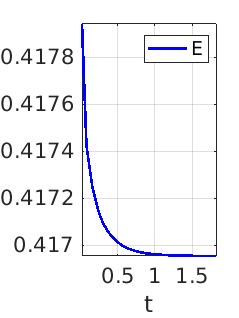
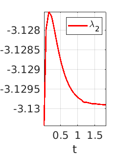
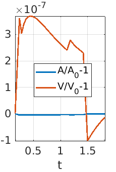
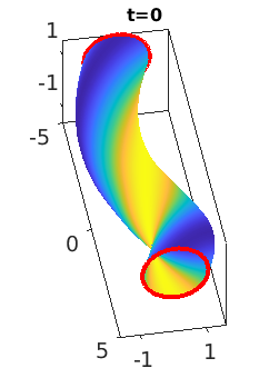
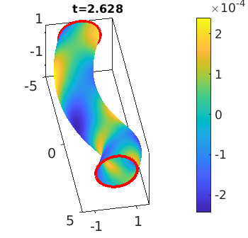
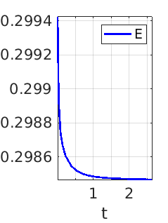
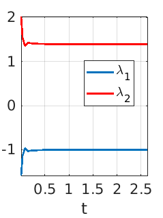
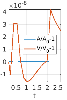
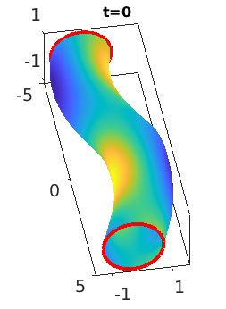
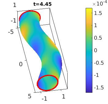
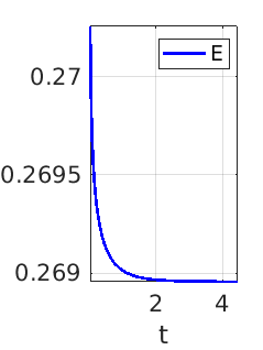
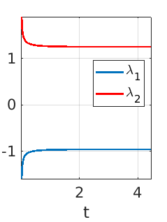
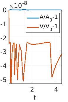
(a), from Fig.4A2   (b), from Fig.4B (c1), from Fig.4C, perturbation by (67) (c2), from Fig.4C, perturbation by (68)

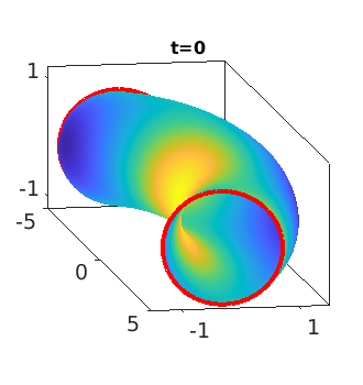
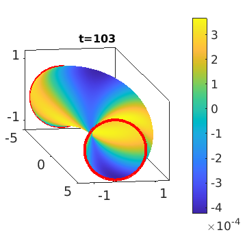
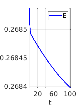
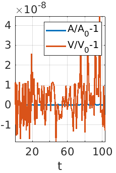
Figure 6: Numerical flows from perturbations of states from Fig.4; initial and ’final’ state, and evolution of $E$, $\lambda_{1,2}$ (only $\lambda_{2}$ in (a) and (c₂)), and deviations from intial area and volume; very slow evolution in (c₂).

The first two flows start near stable steady states $(X_{0},\lambda_{1,0},\lambda_{2,0})$, and as expected flow back to near $X_{0}$ rather quickly, with partly significant changes of $(\lambda_{1},\lambda_{2})$. However, the third flow (c₁) is somewhat surprising. State C from Fig.4 is linearly unstable, but the perturbed $X_{0}$ flows to another buckling by adjusting $\lambda_{1,2}$ at the increased area and volume, where this buckling is stable. On the other hand, in (c₂) for the (linearly) area and volume preserving initial perturbation into the most unstable direction (which point towards coils), the behavior is different: The solution now converges to a coil, with a rather small flow throughout; $\lambda_{1}$ hardly changes at all, $\lambda_{2}$ only very slightly, and the convergence is very slow (since the leading eigenvalue of the target coil is negative but very close to zero). For all flows, we can use the final state as an initial guess for steady state continuation (e.g., in $\lambda_{2}$), and the obtained numerical steady states then are (volume preserving) linearly stable.

Table 1: Spectral data ($n_{\text{unst}}$=number of ($V$-preserving) unstable directions, $\mu_{\text{crit}}$=least stable/most unstable eigenvalue), perturbation parameter $\delta$ ($\xi{=}1$ throughout), and results for DNS in Fig.6; $A_{0}{=}20\pi,V_{0}{=}10\pi$. Initial perturbations for A–C of type (67), and for C^∗ of type (68). $(\lambda_{1},\lambda_{2})_{0}$ are the values at the (perturbed) steady state.

IC type	A2 (pearling)	B (coiling)	C (buckling)	C (buckling)∗
$n_{\text{unst}},\mu_{\text{crit}}$	0, -2.22	0, -0.018	1, 0.012	1, 0.012
$\delta$	-0.125	-0.25	-0.25	0.5
$(A-A_{0})/A_{0}$	0.0012	0.0003	0.0125	0.0024
$(V-V_{0})/V_{0}$	0.0011	0.0004	0.02	0.004
$(\lambda_{1},\lambda_{2})_{0}$	(3.734, -3.165)	(-0.999, 1.387)	(-0.972, 1.29)	(-0.972, 1.29)
$(\lambda_{1},\lambda_{2})_{\text{end}}$	(3.701, -3.133)	(-0.999, 1.389)	(-1.003, 1.367)	(-0.965, 1.25)

(a1) (a2)

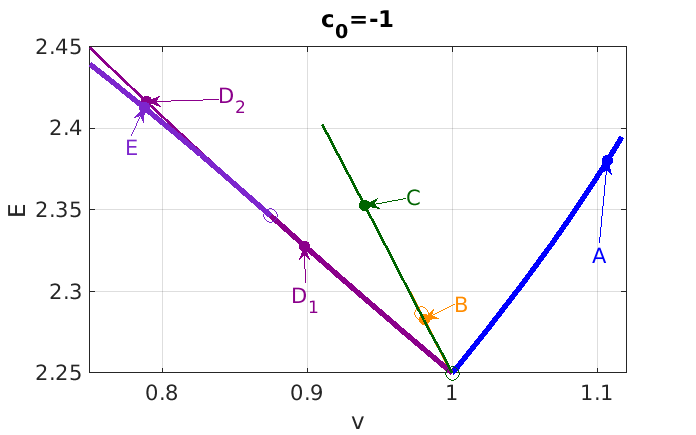
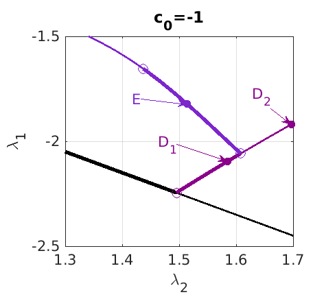
(b)

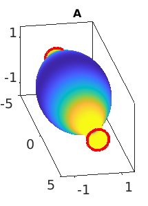
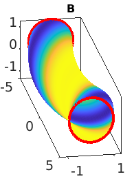
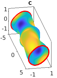
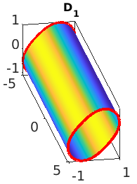
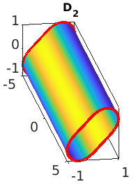
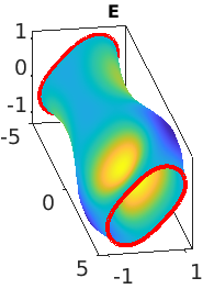
(c)

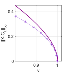
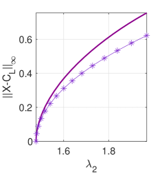
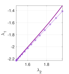
Figure 7: Basic BD (a) for $c_{0}=-1$, $L=10$, and samples (b). (a₁) Energy $E$ over $v$; (a₂) $\lambda_{1}$ over $\lambda_{2}$ for the wrinkling D and ’embedded oblates’ E. (c) Comparison with AE prediction for primary wrinkling.

5.2 $c_{0}=-1$

For (strongly) negative $c_{0}$, the wrinkling branches and their secondary bifurcations become relevant. Fig.7(a,b) shows basic results for $c_{0}{=}-1$ and $L{=}10$, and (c) a comparison with the AE predictions from (62) for wrinkling, again with very good agreement, cf. Remark 5.1. As before, at negative $\lambda_{2}\approx-2.254$ and $\lambda_{1}\approx 1.5$ (cf.Fig.2), $\mathcal{C}_{r}$ looses stability to pearling, but now at positive $\lambda_{2}=3/2$ and $\lambda_{1}=-9/4$ it looses stability to the wrinkling branch (samples D_1,2), while the bifurcation to buckling and coiling is at a later $(\lambda_{1},\lambda_{2})\approx(-3.77,3.021)$ and yields initially unstable branches. The wrinkling is initially stable, but at $\lambda_{2}\approx 1.6$ loose stability to “oblates embedded in wrinkling”, see sample E, and Remark 5.

Figure 8 shows some numerical flows from states from Fig.7, focusing on wrinkling perturbed according to (67) (pearling is again stable, also under rather large perturbations). D₂ at its given $({\cal A}_{0},{\cal V}_{0})$ is linearly (weakly) unstable, and the perturbation yields a slow evolution to an oblate wrinkling, with a very small change in $E$. In (b) and (c) we perturb a coiling and a buckling, and in both cases flow to wrinkling, and the bottom line of Fig.8 and similar experiments is that (stable) wrinkling and oblate wrinkling have rather large domains of attraction.

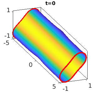
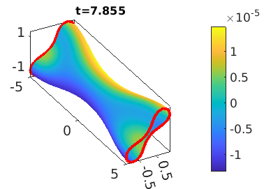
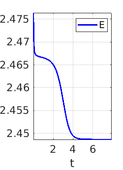
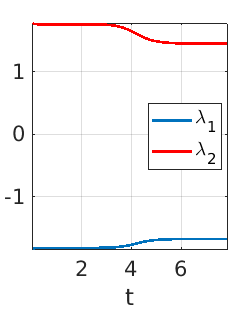
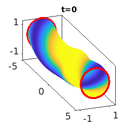
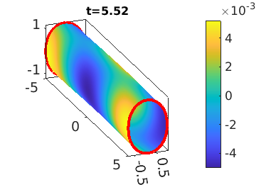
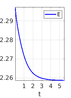
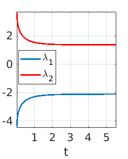
(a), from Fig.7D2 (b), from Fig.7B   (c), from Fig.7C

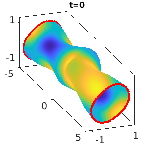
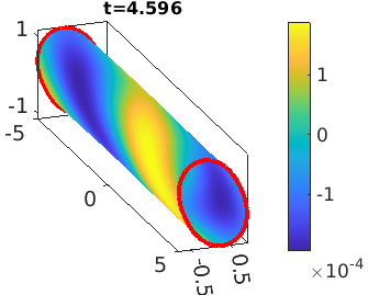
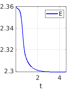
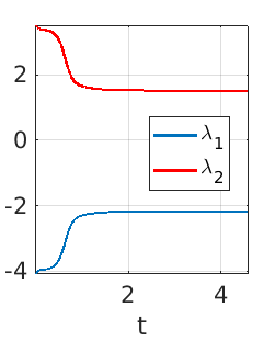
Figure 8: Numerical flows near states from Fig.7; initial perturbations of type (67) with $\delta=-0.25$. Flow to “embedded oblate”, here at the boundary, in (a), and to wrinkling in (b,c).

5.3 $c_{0}=0.48$

Lastly, we consider positive $c_{0}$, specifically $c_{0}=0.48$. By Corollary 3.2, the cylinder destabilizes in a finite wave length pearling instability, and in a long wave instability to coiling and buckling. The finite pearling period is $\ell:=\ell_{p}\approx 7.5$, and thus we will be mostly interested in length $L$ as multiples of $7.5$.

However, for comparison with the cases $c_{0}=0$ and $c_{0}=-1$ we first again choose $L=10$, and in Fig.9 give the BD of buckling and coils. The coefficients for the AE description (64) now are $(a,b_{1},b_{2})=(0.39,-0.083,0.56)$, and in agreement with Fig.3 the buckling are now stable at bifurcation and the coils unstable. Moreover, we find interesting 2ndary bifurcations on both branches, where the buckling looses (coiling gains) stability, and these two BPs are connected by a stable intermediate branch, see sample C. The comparison with the AEs in (c) again shows the agreement close to bifurcation, but naturally the (cubic order) AEs cannot capture the fold of the coiling in $\lambda_{2}$.

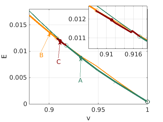
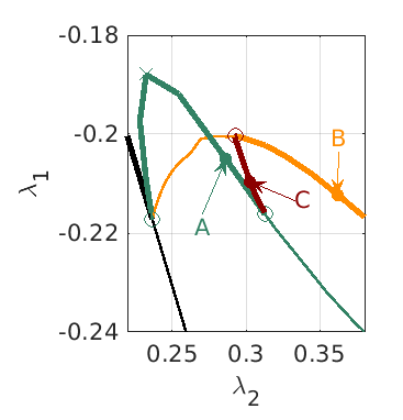
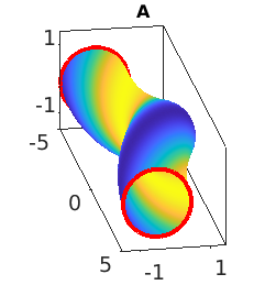
(a) (b) 0mm 0mm

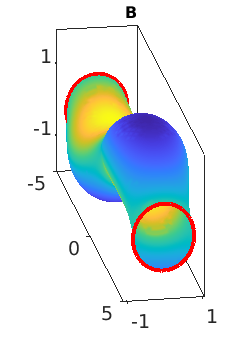
(c) (d) 0mm

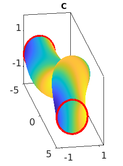
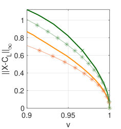
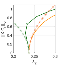
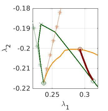
Figure 9: $c_{0}=0.48$, $L=10$. Numerical BDs and samples in (a,b,c), where C shows a stable connection between the stable regimes of coiling and buckling. Comparison to AE predictions in (d).

Figure 10 shows the BD and samples for $L=15$. To the right of $v=1$ bifurcates the $m=2$ pearling branch (at $\lambda_{2}\approx-0.243$), and is initially stable (sample A₁). However, shortly after ($\lambda_{2}\approx-0.3756$) there is a secondary bifurcation to a stable branch with double the period, sample B. On the other hand, the primary $m=1$ pearling branch, sample C, (bifurcating at $\lambda_{2}\approx-0.421$) is unstable throughout. The $(m,n)=(1,1)$ coiling (sample D) and buckling (sample E) bifurcate at $\lambda_{2}\approx 0.138$, and again the coiling is stable, and stays stable to rather small $v$, while the buckling is unstable. Wrinkling does not occur in the parameter regime considered; however, the (compared to $L=10$ before) slightly larger $L=15$ lets the pearling and coiling/buckling BPs move closer together, which is why we chose to present the $(m,n)=(2,1)$ coiling F (unstable). Figure 11 shows the flow from a perturbation of A₂ to a B type solution but rather close to the BP. Therefore, the convergence to steady state is again very slow, as near bifurcation the stable B branch has a leading eigenvalue close to $0$.

(a1) (a2)

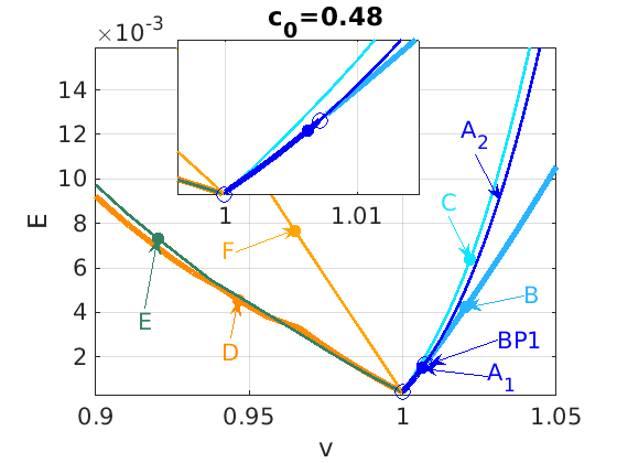
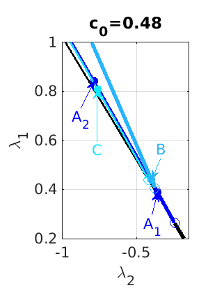
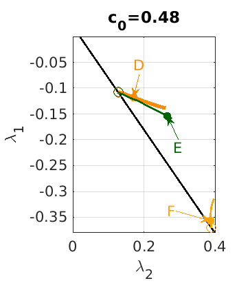
(c)

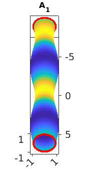
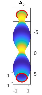
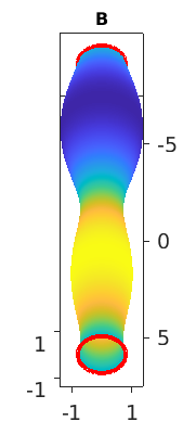
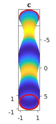
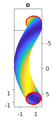
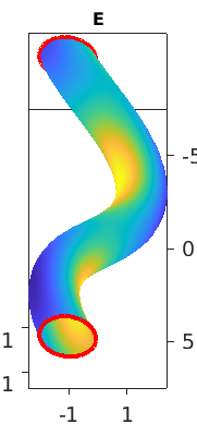
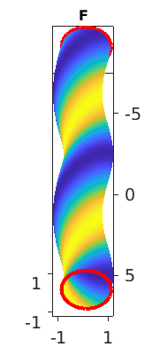
Figure 10: Basic BD for $c_{0}=0.48$, $L=15$. (a) Energy $E$ over reduced volume $v$, and $\lambda_{1}$ over $\lambda_{2}$. (b) Samples from primary pearling, A₁ stable, A₂ unstable. (c) further samples: B is period doubling from A branch, stable; C is the primary $m=1$ pearling bifurcation, unstable; D is a (1,1)–coiling, stable; E is a (1,1)–buckling, unstable; F is a (2,1)–coiling.

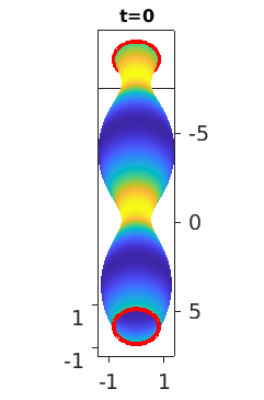
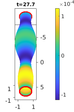
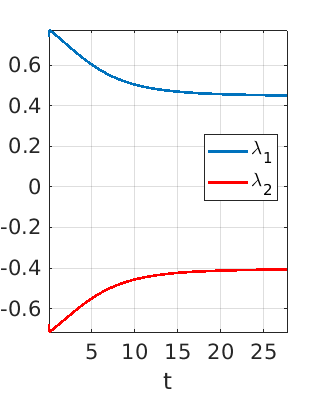
Figure 11: Sample flow from perturbation of A₂ of type (68) with $\delta=0.5$, going to B type solution.

The main point of Fig.10 is that the choice of $c_{0}=0.48$ together with $L=15$ yields the destabilization of the cylinder to the $m=2$ pearling, but these solutions are only stable in a somewhat narrow range (in $v$, say). To further assess this, in Fig.12 we consider the primary pearling with $\ell=7.5$ on twice the domain $L=30$. The result shows that the range of stable $\ell=7.5$ pearls shrinks with increasing $L$, and this continues for further increase of $L$, yielding the following dependence of the reduced volume $v_{s}$ of single pearling BPs from primary $\ell=7.5$ pearling on $L$:

$$L$$ 15 39 45 60

1.0081 1.0063 1.0046 1.0035

(71)

We also ran some numerical flows from perturbations of A in Fig.12, and similarly at larger $L$, with results as in Fig.11, i.e., convergence to the single pearl solutions. However, these DNS are very expensive, partly due to the larger domain and hence larger scale discretization, but more importantly due to the very slow convergence of the flows.

(a) (b)

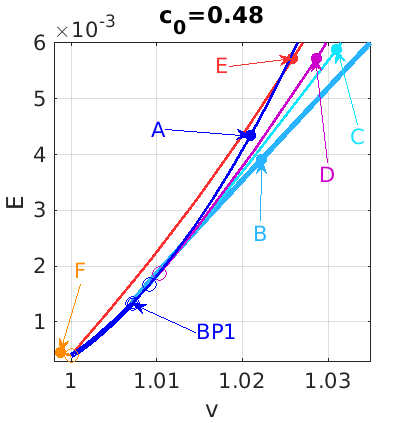
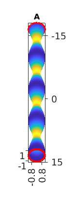
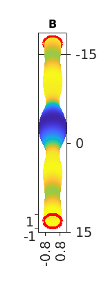
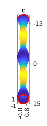
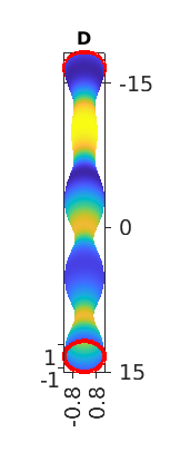
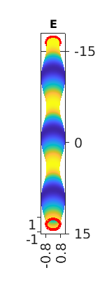
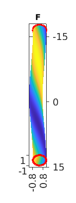
Figure 12: $c_{0}=0.48$, $L=30$. The $m=4$ (period $\ell=7.5$) pearling A now looses stability at BP1 much closer to its primary bifurcation, to a single “localized” pearling branch, sample B. Further branches: C: $m=2$ ($\ell=15$) primary pearling; E: $m=3$ ($\ell=10)$ primary pearling; D: 2ndary pearling from 2nd BP on $m=1$ branch. F: primary $(m,n)=(1,1)$ coiling.

Appendix A Appendix

A.1 Numerical continuation via pde2path

The basis of the numerical setup is explained in [MU24] partially recalled below and adaptations are described. The legacy version of those algorithms are downloadable at [Uec24] and the source of this implementation is given in the supplementary martial (pde2pathrequired). For the numerical implementation, we recall some discrete differential geometric operators, mostly from [MDSB03]. Let (X, tri) a triangulation of the immersed surface $X$. Here node coordinates are X${}_{j}\in{\mathbb{R}}^{1\times 3}$ with $j\in\{1,\ldots,n_{p}\}$ ($n_{p}$ is the number of points) and tri$\in{\mathbb{R}}^{n_{t}\times 3}$ ($n_{t}$ us the number of triangles). Using linear hat functions $\phi_{i}:X\rightarrow{\mathbb{R}}$ with $\phi_{i}($X${}_{j})=\delta_{ij}$ with $i\in\{1,\ldots,n_{p}\}$, the operator

$$L_{kl}=\int_{X}\nabla\phi_{k}\nabla\phi_{l}\,{\rm d}S=-\frac{1}{2}(\cot\alpha_{kl}+\cot\beta_{kl}).$$ (72)

The stability analysis here is done in a slightly different setting as in the legacy version of pde2path. Usually the stability is checkt for the given active parameter set p.nc.ilam.m, in our case $(\lambda_{1},\lambda_{2},\text{PC})$, where PC stands for the Lagrange multipliers of the phase conditions, where the primary $\lambda_{1}$ is assumed to be fixed. However in the dynamical problem, the Lagrange multipliers are in general time dependent. The disinherit, stability information is for fixed $A$ and $V$. Hence after a successful continuation step, a new Jacobian is build according to the p.nc.ilam$=(V,\lambda_{1},\lambda_{2},\text{PC})$.

Remark .

During the continuation of bifurcating branches, it is not necessary that the boundary of $X$ stays in a plane, similar to the cylinder. This however is allowed and makes no problem in the continuation. But for mesh refinement along the branch the legendary box2per setting looks for periodic boundary nodes in a plane. For that reason we only allow an $(y,z)$ displacement at the boundary, by setting $N_{x}=0$. Note that the computations for $H(X)$ this is not done for accurate computations also at the boundary.

A.1.1 Mesh handling

The initial cylinder in discretized by a standard mesh from pde2path, mapped via a local map on the cylinder. The number of nodes in $x$ and $y$ direction is chosen that the quotient

$$q=\frac{e_{M}}{R},$$ (73)

with $e_{M}$ the maximal edge length and $R=A/C$ the ratio of area and circumcenter, is minimal. The triangulation is oriented inwards, matching with the above convention.
On the bifurcation branches some triangles may distort, due to the change of X. We establish an mesh adaption consisting of refinement and coarsening of X and tri from the prior step wrt. the periodic boundary nodes. As a control function we use the are of a triangle and refine the area is above a threshold. This is typically 1.3 times the size of a triangle on the original cylinder.The refinement algorithm Trefinelong.m is based on the RGB refinement in [FS21], but force that the longest side has to be refined, see LABEL:reffig(b) , creating a mesh with valences 4 and 8. However this increases (73) in a regular sized mesh, while for acute triangles the refinement produces two obtuse ones. A retriangulation retrigX.m swaps edges so we get only valence 5 or 6 and lowers (73) again, see LABEL:reffig(c) , except at the boundary, see [PS04]. However this strategy has proven to be the most efficient way, in order to avoid long cascades of triangles from the RGB refinement. For the conservation of the periodic boundary, we enforce the same refinement at both boundary triangles. In some cases one boundary side is refined while the local structure do not allow the same refinement at a the other boundary. In that case we collapse the excess node along the side of its nearest boundary neighbor.
For the coarsening (73) is the control parameter, activated if $q>8$. The strategy select triangles smaller then a threshold $A_{t}$, (legacy version max(A)/2, but set to max(A)/3 and acute (ratio of circumcenter to area) as coarsened triangles. Then the obtuse neighbor triangles of those are found. The acute triangles are collapsed along the shortest edge. Then edges are flipped until one gets a triangular mesh. This is iterated as long as all triangles are larger than $A_{t}$.

References

- [CL00] P. Chossat and R. Lauterbach. Methods in equivariant bifurcations and dynamical systems. World Scientific Publishing Co., Inc., River Edge, NJ, 2000.
- [FS21] S. A. Funken and A. Schmidt. A coarsening algorithm on adaptive red-green-blue refined meshes. Numer. Algorithms, 87(3):1147–1176, 2021.
- [FVKG22] B. Foster, N. Verschueren, E. Knobloch, and L. Gordillo. Pressure-driven wrinkling of soft inner-lined tubes. New J. Phys., 24(January):Paper No. 013026, 15, 2022.
- [GNPS96] R.E. Goldstein, P. Nelson, T. Powers, and U. Seifert. Front progagation in the pearling instability of tubular vesicles. J.Phys.II, 6:767–796, 1996.
- [GS02] M. Golubitsky and I. Stewart. The symmetry perspective. Birkhäuser, Basel, 2002.
- [Hel73] W. Helfrich. Elastic properties of lipid bilayers: Theory and possible experiments. Zeitschrift für Naturforschung, 28:693, 1973.
- [Hoy06] R.B. Hoyle. Pattern formation. Cambridge University Press., 2006.
- [JSR93] F. Jülicher, U. Seifert, and R.Lipowsky. Phasediagrams and shape transformations of toroidal vesicles. J.Phys.II, 3:1681–1705, 1993.
- [KN06] Yoshihito Kohsaka and Takeyuki Nagasawa. On the existence of solutions of the Helfrich flow and its center manifold near spheres. Differential and Integral Equations, 19(2):121 – 142, 2006.
- [KPW10] Matthias Köhne, Jan Prüss, and Mathias Wilke. On quasilinear parabolic evolution equations in weighted -spaces. J. Evol. Equ., 10(2):443–463, 2010.
- [LS13] Jeremy LeCrone and Gieri Simonett. On well-posedness, stability, and bifurcation for the axisymmetric surface diffusion flow. SIAM J. Math. Anal., 45(5):2834–2869, 2013.
- [LS16] Jeremy LeCrone and Gieri Simonett. On the flow of non-axisymmetric perturbations of cylinders via surface diffusion. J. Differential Equations, 260(6):5510–5531, 2016.
- [Lun95] A. Lunardi. Analytic semigroups and optimal regularity in parabolic problems. Birkhäuser Verlag, Basel, 1995.
- [MDSB03] M. Meyer, M. Desbrun, P. Schröder, and A. H. Barr. Discrete differential-geometry operators for triangulated 2-manifolds. In Visualization and mathematics III, Math. Vis., pages 35–57. Springer, Berlin, 2003.
- [MRS13] M. Meyries, Jens D. M. Rademacher, and E. Siero. Quasi-linear parabolic reaction-diffusion systems: A user’s guide to well-posedness, spectra, and stability of travelling waves. SIAM J. Appl. Dyn. Syst., 13:249–275, 2013.
- [MU24] Alexander Meiners and Hannes Uecker. Numerical continuation and bifurcation for differential geometric PDEs. Numer. Math. Theory Methods Appl., 17(3):555–606, 2024.
- [NT03] T. Nagasawa and I. Takagi. Bifurcating critical points of bending energy under constraints related to the shape of red blood cells. Calc. Var. PDEs, 16(1):63–111, 2003.
- [PP22] B. Palmer and Á. Pámpano. The Euler-Helfrich functional. Calc. Var. Partial Differential Equations, 61(3):Paper No. 79, 28, 2022.
- [PS04] P. Persson and G. Strang. A simple mesh generator in matlab. SIAM Review, 46(2):329–345, 2004.
- [Sim95] Gieri Simonett. Center manifolds for quasilinear reaction-diffusion systems. Differential and Integral Equations, 8(4):753 – 796, 1995.
- [Uec24] H. Uecker. www.staff.uni-oldenburg.de/hannes.uecker/pde2path, 2024.
- [ZcH89] Ou-Yang Zhong-can and Wolfgang. Helfrich. Bending energy of vesicle membranes: General expressions for the first, second, and third variation of the shape energy and applications to spheres and cylinders. Physical review. A, General physics, 39 10:5280–5288, 1989.