CuPID: Leveraging Masked Single-Lead ECG Modelling
for Enhancing the Representations

Abstract

Wearable sensing devices, such as Electrocardiogram (ECG) heart-rate monitors, will play a crucial role in the future of digital health. This continuous monitoring leads to massive unlabeled data, incentivizing the development of unsupervised learning frameworks. While Masked Data Modelling (MDM) techniques have enjoyed wide use, their direct application to single-lead ECG data is suboptimal due to the decoder’s difficulty handling irregular heartbeat intervals when no contextual information is provided. In this paper, we present Cueing the Predictor Increments the Detailing (CuPID), a novel MDM method tailored to single-lead ECGs. CuPID enhances existing MDM techniques by cueing spectrogram-derived context to the decoder, thus incentivizing the encoder to produce more detailed representations. This has a significant impact on the encoder’s performance across a wide range of different configurations, leading CuPID to outperform state-of-the-art methods in a variety of downstream tasks.

1 Introduction

The wearable sensing field has seen remarkable advancements in recent years, and is expected to play a crucial role in the future of digital health. One widely used type of wearable health sensor is the heart monitor that captures cardiac activity as single-lead Electrocardiogram (ECG) signals during free-living conditions, such as in the patient’s home. Mapping these signals with significant clinical outcomes has the potential to provide outstanding benefits such as simplifying the diagnostic process (Himmelreich et al., 2019) or enabling users to engage proactively in tracking their cardiac health (Abdou & Krishnan, 2022). In this context, models that extract information from single-lead ECG into generalizable representations are mandated to address distinct downstream tasks. In addition, this continuous monitoring leads to massive unlabeled datasets. This makes Self-Supervised Learning (SSL) framework particularly well-suited for addressing this clinical challenge.

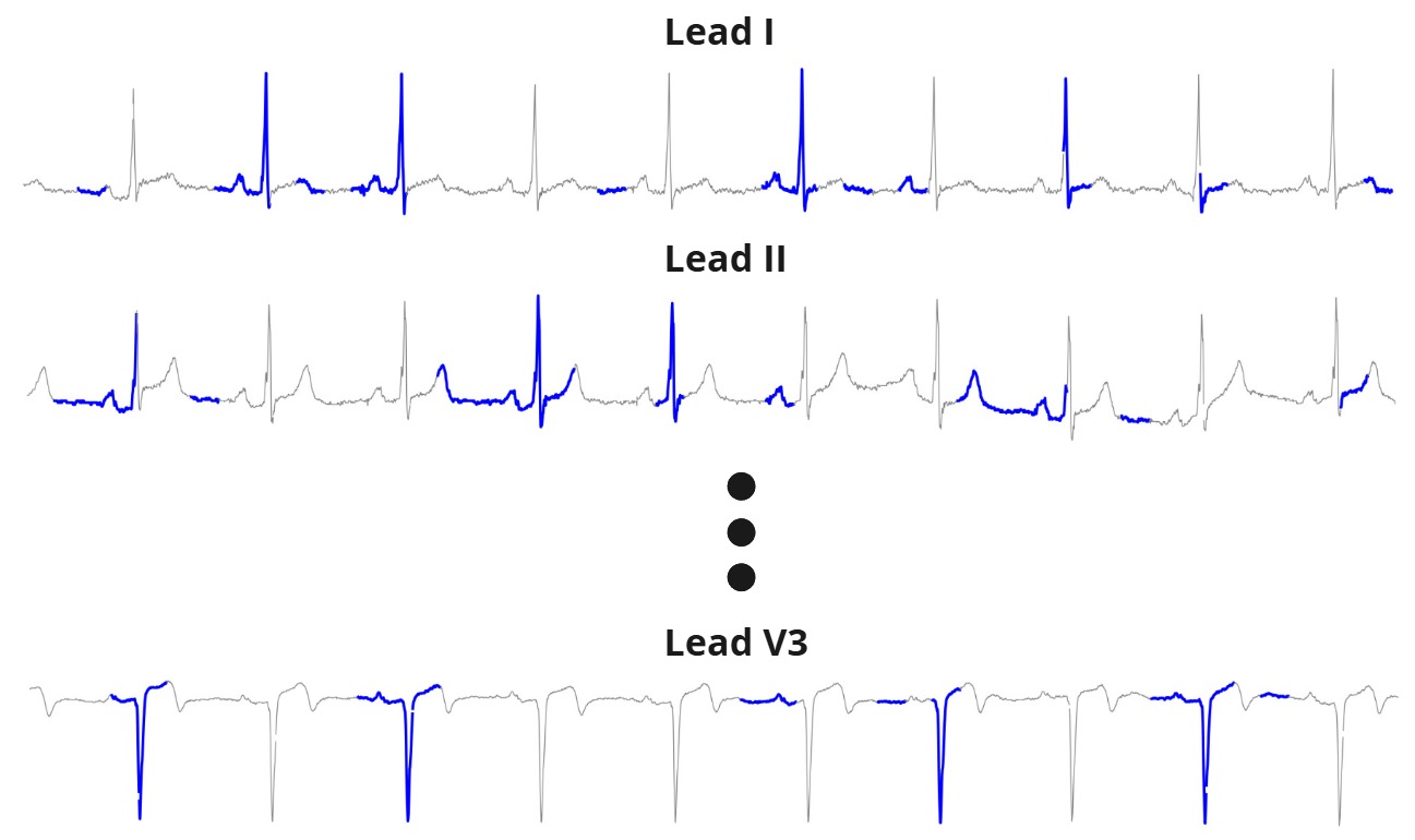
Figure 1: Example of the commonly used masking strategy proposed in (Na et al., 2024) for 12-Lead ECG processing. Unmasked portions are displayed in blue. Most of the ECG waves remain unmasked in at least one of the leads.

Recently, Masked Data Modelling (MDM) methods have been gaining attention in the SSL field (He et al., 2021; Gupta et al., 2023; Assran et al., 2023). They rely on masking a portion of the input and driving a transformer-based encoder, typically a Vision Transformer (ViT) (Dosovitskiy et al., 2021) to compute detailed representations that enable a decoder to infer the unseen patches. In the realm of 12-lead ECG processing, MDM methods have been applied recently with promising results (Na et al., 2024). They prove that independently masking the different leads outperforms the strategy of consistently masking across time proposed in Masked Time Autoencoder (MTAE) (Zhang et al., 2023).

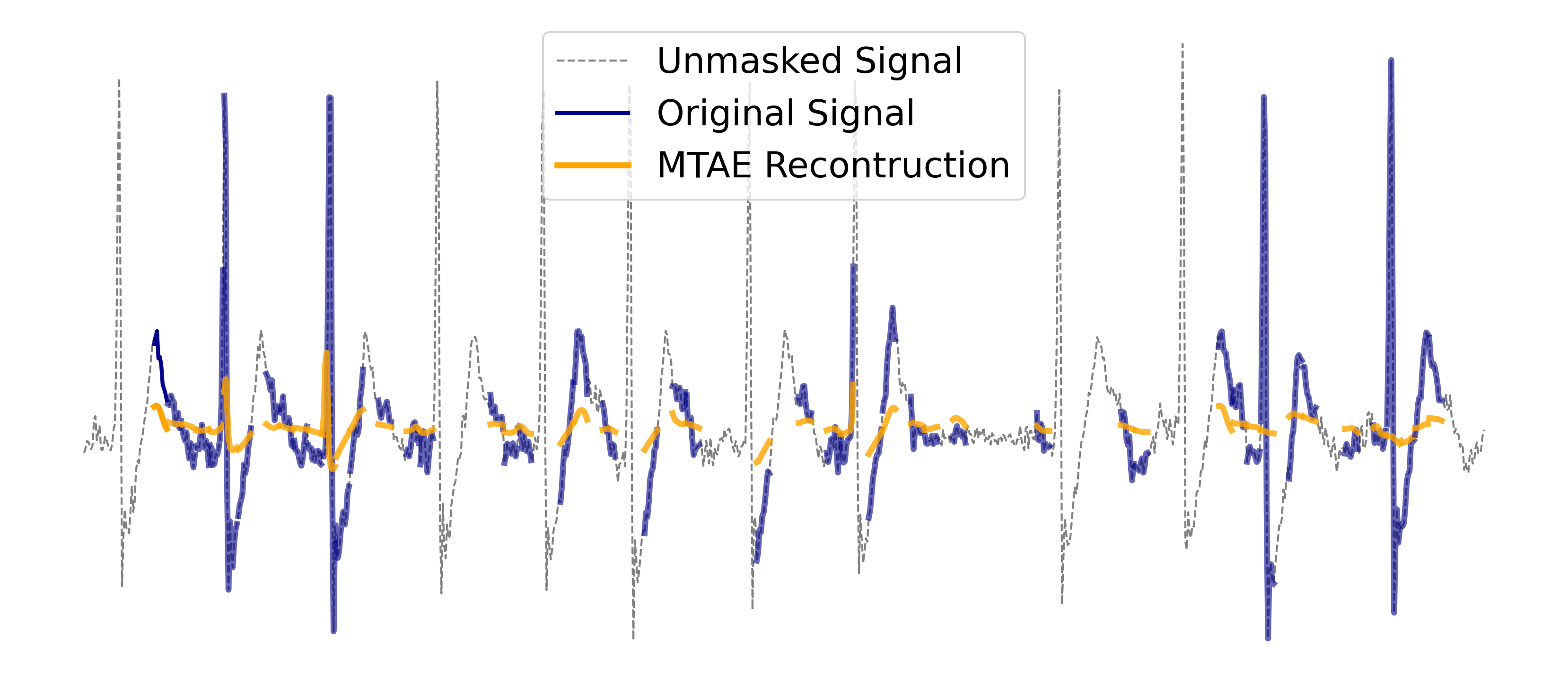
(a)

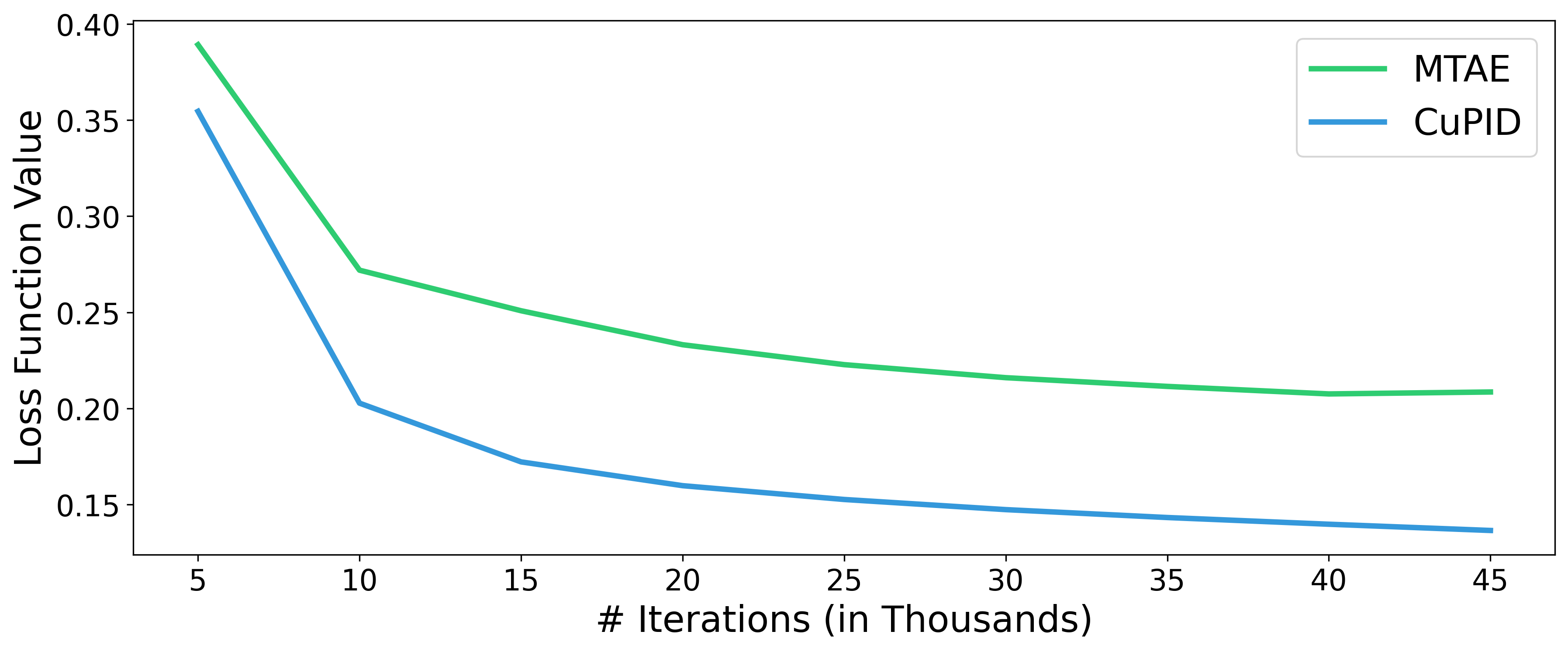
(b)

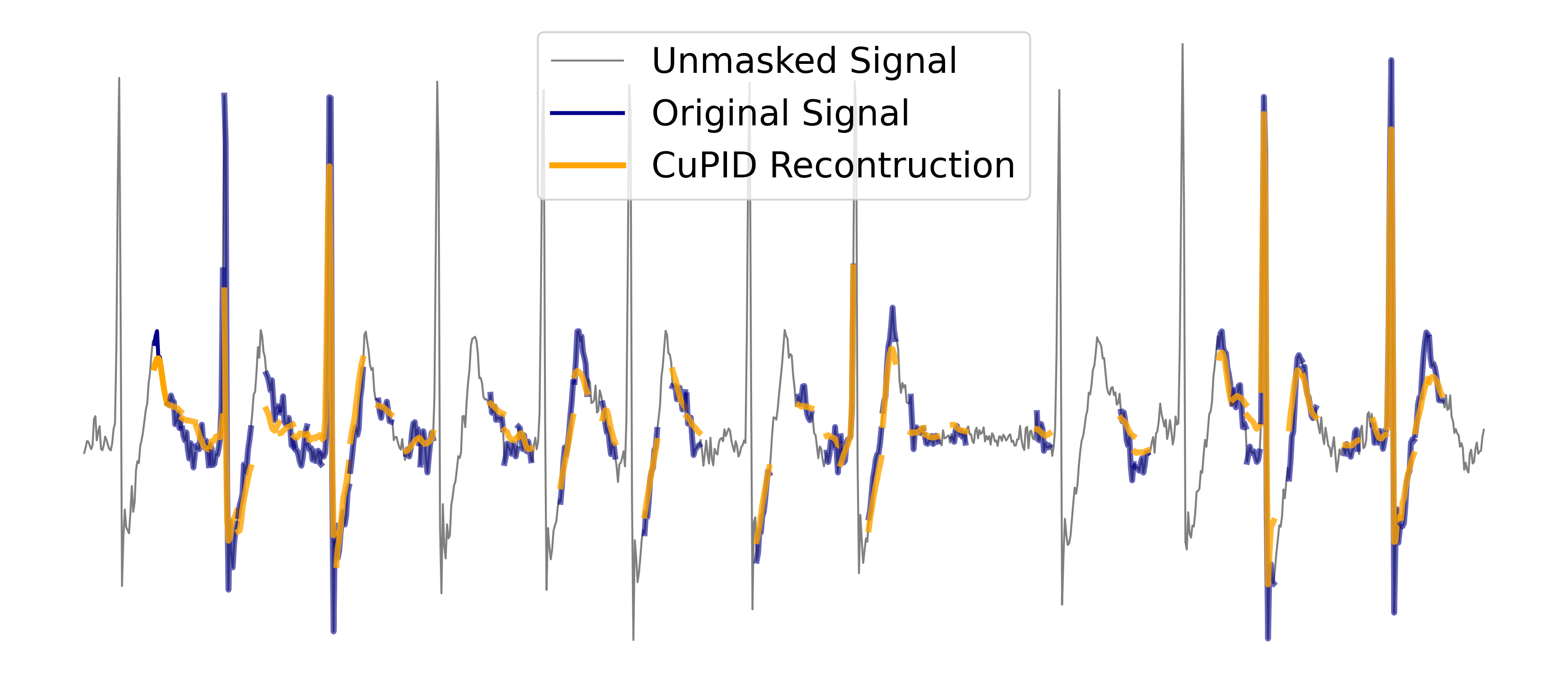
(c)

(d)

Figure 2: Reconstruction comparison between CuPID and MTAE. Figures 2(a) and 2(c) display a reconstruction from MTAE and CuPID, where the unmasked part, the ground truth, and the inference computed by both methods are represented in gray, blue, and orange, respectively. Figure 2(b) illustrates loss function evolution across pre-training. Figure 2(d) compares the performance of CuPID and MTAE, across different heartbeat irregularity levels, measured in SDNN (Standard Deviation of Normal Intervals).

This lead-independent masking strategy, represented in Figure 1, allows the encoder to model the temporal positions of the distinct ECG waves by integrating the unmasked portions of the various leads. This contextual information is crucial, as it enables the decoder to deal with fluctuations in the time intervals between heartbeats. However, this masking strategy can not be applied to single-lead ECG data, our data of interest, which just accommodates one signal. The decoder encounters challenges in handling irregular heartbeat intervals, as it lacks contextual information from other leads. Since not inferring exactly this position has a big impact on the loss, the decoder is cautious when reconstructing the masked patches. Figure 2(a) displays how it estimates a value near the average rather than matching precisely the signal’s morphology.

This paper presents Cueing the Predictor Increments the Detailing (CuPID), which is a novel SSL method that addresses the issue mentioned above by cueing the decoder with contextual information provided by the spectrogram of the input signal. The spectrogram is expected to mirror the contextual information provided by other leads in the 12-Lead ECG framework. It is fed into the attention mechanism of the decoder as the Key (K) to ensure that its role is merely informative and its value can not be used directly to reconstruct the representations. It leads to a significant decrease in the loss function values, as shown in Figure 2(b), and reconstructions are adjusted more to the morphology of the original signal, as captured in Figure 2(c). Figure 2(d) shows how this behavior is consistent across different levels of irregularity in heartbeat intervals.

Although these results are insignificant on their own since CuPID’s decoder is provided with additional information, we hypothesize: (I) The decoder’s inability to reconstruct the original signal due to the irregularity in the heartbeat intervals limits the encoder’s learning potential. (ii) Cueing the decoder with the spectrogram endows it with the potential to solve the task. It drives the encoder to compute detailed patch representations which can be used to accurately reconstruct the input. (iii) The more informative the patch representations are, the more performant the encode will be at the time of addressing downstream tasks.
To assess our hypothesis, we have conducted an extensive evaluation where CuPID is compared against the existing state-of-the-art SSL methods tailored for single-lead ECG analysis. Up to three distinct databases; MIT-BIH Atrial Fibrillation (MIT-AFIB) (Moody & Mark, 1983), Physionet Challenge 2017 (Clifford et al., 2017), and Long Term AF (LT-AF) (Petrutiu et al., 2007), are considered. Remarkably, CuPID achieves significantly superior performance when compared with single-lead ECG methods. Finally, the benefit of incorporating the spectrogram compared with the MTAE baseline is assessed for different configurations.

In summary, the contributions of this paper are:

• We have discussed the limitations of applying MDM techniques directly to single-lead ECG signals due to the idiosyncrasy of this kind of data.

• We introduce CuPID, a novel SSL method that addresses these limitations by helping the decoder during the pre-training. This is made by incorporating the spectrogram of the input signal to the attention mechanism as the Key, limiting its role to be merely informative.

• We provide a model that achieves markedly enhanced results in a variety of downstream tasks that are relevant for cardiovascular remote monitoring.

2 Related Work

2.1 Masked Data Modelling (MDM)

Masked Data Modelling (MDM) has been a commonly used technique in the Natural Language Processing (NLP) field. Methods such as Bidirectional Encoder Representations from Transformers (BERT) (Devlin et al., 2019) that rely on hiding a series of words within a sentence and optimizing a decoder to infer these words have proven to be the most effective pre-training method in the field.

In recent times, this pre-training mechanism has been adapted in the field of computer vision. Existing methods, such as, Masked Autoencoders (MAE) (He et al., 2021) or Siamese Masked Autoencoders (SiamMAE) (Gupta et al., 2023) incorporate a decoder trained to reconstruct masked patches from the original input. This approach has shown promising results in the field of computer vision, outperforming gold-standard Energy-Based Modelling (EBM) methods such as Variance-Invariance-Covariance Regularization (VIC-REG) (Bardes et al., 2022), Self-Distillation with no Labels (DINO) (Caron et al., 2021), or Bootstrap Your Own Latent (BYOL) (Grill et al., 2020).

2.2 SSL in 12-Lead ECG Signal Processing

In the realm of 12-lead ECG signals, research has effectively utilized the MDM framework. The availability of various leads broadens the scope for the strategy of input masking. Techniques like MTAE, MLAE, and MLTAE, all introduced by MAE family of ECG (MaeFE) (Zhang et al., 2023), suggest three masking strategies: temporal masking, spatial masking across different leads, or a combination of both. Spatio-Temporal Masked Electrocardiogram Modeling (ST-MEM) (Na et al., 2024) reaches the state-of-the-art performance by employing a joint decoder that reconstructs the original input attending to each lead independently. It proves that adopting this combined strategy by independently masking the different leads achieves the best results.

Among the four listed methods, only MTAE is suitable for single-lead ECG signals, as the other three require multiple leads. MTAE is not only included in the evaluation, but also in the ablation studies since this method is CuPID’s analogous version without the use of the spectrogram.

2.3 SSL in Single-Lead ECG Signal Processing

Most-widely used single-lead ECG SSL methods follows a EBM approach; (i) Contrastive Learning of Cardiac Signals Across Space (CLOCS) (Kiyasseh et al., 2021) utilizes two consecutive ECG time strips as positive pairs, (ii) Mixing-Up (Wickstrøm et al., 2022) introduces a more tailored data augmentation product of two time series from the same recording, (iii) Patient Contrastive Learning (PCLR) (Diamant et al., 2022) which considers two time strips from the same subject but different recordings. While all these methods utilize the Contrastive Learning (Chen et al., 2020) as a common framework for learning the invariant attributes considering non-overlapping inputs as positive pairs, Distilled Embedding for Almost-Periodic Time Series (DEAPS) (Atienza et al., 2024) follows a non-contrastive learning approach. (iv) It drives the model to capture the also dynamic patterns of the single-lead ECGs.

All of these SSL methods will compose the set of baselines for the CuPID’s evaluation, where the representations computed by each pre-trained model will be employed for addressing several downstream tasks.

2.4 Use of Spectogram for ECG Processing

Spectrograms have enjoyed wide use in ECG signal processing due to their ability to provide a time-varying spectral density description of the data. Consequently, it is often used as a substitute for the ECG signal as input for deep learning models designed to address various arrhythmia classification tasks (Eleyan et al., 2024; Bing et al., 2022). Additionally, the spectrogram can be treated as an image, enabling the application of SSL techniques developed for computer vision to this type of data (Thinh et al., 2022).

All the previously mentioned methods actively utilize the spectrogram to map input to clinical outcomes. CuPID stands out since the spectrogram is only employed during pre-training to provide the decoder with the temporal context of the ECG waves. The encoder does not receive the spectrogram, and thus, it is not used during inference.

3 Cueing the Predictor Increments the Detailing (CuPID)

Figure 3: CuPID architecture. The left side of the Figure shows how the spectrogram is incorporated into the decoder’s attention mechanism. This incorporation sets CuPID apart from the standard framework for MDM. The encoder is the model used to address the downstream tasks, while the decoder is discarded after the pre-training. Therefore, this spectrogram is not provided during the evaluation. The right side of the diagram provides a closer look at CuPID’s decoder. Due to the challenges of using the spectrogram as a Key, the spectrogram is incorporated from the second block of the decoder. Its first block mirrors the standard decoder block for MDM framework.

The core idea behind CuPID is cueing the decoder with the contextual information provided by the spectrogram. Its workflow is illustrated in Figure 3. From left to right the original signal input is patched and embedded using a linear layer. A portion of these tokens (Represented as gray blocks in the figure) is randomly masked with a fixed ratio. Only the unmasked tokens are passed through the encoder. Learnable mask tokens with their respective positional encoding are placed in the original position of the masked segments. What sets CuPID apart is that it uses the spectrogram as the Key for the attention mechanism, as represented in Figure 3. This decoder reconstructs the original input. The $\mathcal{L}_{1}$ metric is computed between this reconstruction and the original input. This loss function is only calculated on the masked patches. It is important to note that the decoder is discarded after training, with the encoder being used for downstream tasks. Therefore, the spectrogram is only utilized during pre-training and not during inference.

3.1 Role of Spectrogram for the decoder

Due to the lack of contextual information, the baseline decoder faces challenges when handling irregular heartbeat intervals. The core idea behind CuPID is to provide the decoder with the needed contextual information from an alternative source. The spectrogram is identified as an effective tool for this purpose. This section delves deeper into the rationale behind this decision and its implementation.

Spectrogram as Choice:

A spectrogram is a visual representation of the spectrum of frequencies in a signal as they vary over time. They are commonly generated using the Fast Fourier Transform (FFT), which converts a time-domain signal into its frequency components.

We identify the spectrogram as a tool that has the potential to provide the decoder with the needed contextual information since: (i) The spectrogram retains the temporal aspect of the signal, allowing us to isolate the frequency component of each patch by dividing it into consistent patches aligned with the original input ones. (ii) The distinct waves accommodated in the ECG signal operate in distinct frequencies. This feature is leveraged by traditional signal processing methods to perform ECG signal delineation (Martinez et al., 2004). Therefore, by providing the frequency component of each mask token, the decoder can determine if a wave is present there and identify the kind of wave it should reconstruct.

Limiting the Information Provided by the Spectrogram:

Just as the time domain input is transformed into the frequency domain when computing the spectrogram, it can also be converted back to the time domain. It means that the decoder could potentially reconstruct the original input without using the encoder’s representations. To prevent this, the spectrogram is used just as the K in the attention mechanism when fed into the decoder. This transformer-based decoder relies on the standard attention mechanism formulated on (Vaswani et al., 2017). It is composed of three components, i.e., query ($Q$), key ($K$), and value ($V$) and it is expressed as the following:

$$\operatorname{Attention}(Q,K,V)=\operatorname{softmax}\left(\frac{QK^{T}}{\sqrt{d_{k}}}\right)V,$$ (1)

where the query ($Q$) refers to the token that is attending the others for information, the key ($K$) represents what information can be found in the specific token, and the value ($V$) accommodates the information. It is worth highlighting that the $K$ only has the potential of informing what kind of information it could be found in the respective token, but not providing information by itself. This information is provided by the corresponding $V$. In other words, even though the spectrogram gathers all the information needed for reconstructing the input, this information can not be applied directly.

Challenges of Using the Spectrogram as the Key:

CuPID does not mask the spectrogram when fed into the decoder. The purpose of incorporating the spectrogram is to enhance mask tokens with contextual information about the temporal location and the kind of ECG waves each accommodates for an accurate reconstruction. Therefore, masking the spectrogram would be counterproductive.

However, a primary issue arises when using the spectrogram without masking it. Since this spectrogram is fed as the K into the attention mechanism of the decoder, it cannot distinguish between informative tokens and mask tokens, as this distinction is not present in the spectrogram. Therefore, a token might be retrieving information from a mask token even when it is merely a mask and contains no actual information. To overcome this issue, CuPID delays incorporating the spectrogram into the decoder’s second block. Consequently, the regular concatenation of encoder representations and mask tokens is used as the K in the first encoder block. By doing this, CuPID ensures that each mask token retains some information after the initial block, which can then be distilled in subsequent blocks with the context information provided by the spectrogram.

Decoder Workflow and Loss Function:

Considering these two crucial aspects, Figure 3 depicts the CuPID decoder. In the initial block, the inference follows a conventional approach, while the spectrogram is integrated into subsequent blocks as the $K$ in the attention mechanism. This decoder computes the single-lead ECG reconstruction, which is compared to its corresponding original input using the $\mathcal{L}_{1}$ metric. This metric serves as the sole loss function of the model and is represented by the following formula:

$$\mathcal{L}_{1}(X,\hat{Y},\mathcal{M})=\frac{1}{sum(\mathcal{M})}\cdot\sum_{i=1}^{n}\left|Y_{i}-\hat{Y}_{i}\right|\cdot\mathcal{M}_{i},$$ (2)

where $X$, $\hat{Y}$, $\mathcal{M}$, and $n$ represent the original input, the decoder reconstruction, the mask, and the number of patches.

3.2 Implementation Details

To ensure the replication of the method, we meticulously outline the hyperparameter configuration.

Model Architecture: As is standard practice when evaluating MDM approaches, the standard ViT (Dosovitskiy et al., 2021) architecture is used as the encoder module. To align the encoder size with the data complexity and meet the efficiency requirements for constant monitoring, CuPID introduces a very lightweight model. In detail, the ViT architecture proposed by CuPID for processing the single-lead ECG signals count with four regular transformer blocks with four heads each and a model dimension of 128. The input consists of a one-dimensional 10-second signal sampled at 100 Hz. This signal is split into patches with a length of 20 samples. The influence of the patch size is studied in Section 5.

CuPID Implementation and Optimization: The decoder consists of a ViT model with two blocks and a dimension of 128. The training procedure consists of 45,000 iterations. We use a batch size of 256, AdamW (Loshchilov & Hutter, 2019) optimizer with a learning rate of $1e-3$. To compute the spectrogram consistent with both the decoder dimensions and the patch length, the number of coefficient bins is set to 255 and the window length to 40. The masking ratio is set to 0.4. The masking ratio and the length of the training process have been determined by a sensitivity study (See Section 5). The training procedure and the evaluations are performed on a desktop computer, with a Nvidia GeForce RTX 3070 GPU.

4 Evaluation

To assess our hypotheses, we have conducted an extensive evaluation. This included five different baselines from key studies in single-lead ECG processing, three commonly used benchmarking datasets, and both linear probing and fine-tuning experiments. This section presents the details of the evaluation, along with the results and their discussion.

4.1 Baselines.

Table 1: Performance comparison of various methods under linear probing and fine-tuning on three ECG datasets. Best values in bold and second best underlined.

	MIT-AFIB			LT-AF			Physionet 2017
Methods	Accuracy	F1	AUC	Accuracy	F1	AUC	Accuracy	F1	AUC
Linear Probing
PCLR	0.691 $\pm$ 0.113	0.636 $\pm$ 0.095	0.731 $\pm$ 0.113	0.808 $\pm$ 0.058	0.568 $\pm$ 0.048	0.869 $\pm$ 0.034	0.6454 $\pm$ 0.0104	0.5597 $\pm$ 0.0094	0.7621 $\pm$ 0.0129
Mix-Up	0.691 $\pm$ 0.056	0.579 $\pm$ 0.232	0.746 $\pm$ 0.103	0.813 $\pm$ 0.045	0.593 $\pm$ 0.060	0.889 $\pm$ 0.031	0.6546 $\pm$ 0.0186	0.5817 $\pm$ 0.0188	0.7906 $\pm$ 0.0109
DEAPS	0.790 $\pm$ 0.079	0.687 $\pm$ 0.189	0.851 $\pm$ 0.100	0.829 $\pm$ 0.045	0.592 $\pm$ 0.051	0.893 $\pm$ 0.033	0.6791 $\pm$ 0.0126	0.6228 $\pm$ 0.0081	0.7897 $\pm$ 0.0082
CLOCS	0.680 $\pm$ 0.088	0.567 $\pm$ 0.218	0.709 $\pm$ 0.108	0.748 $\pm$ 0.023	0.534 $\pm$ 0.032	0.843 $\pm$ 0.032	0.6117 $\pm$ 0.0112	0.4650 $\pm$ 0.0186	0.7473 $\pm$ 0.0135
MTAE	0.808 $\pm$ 0.937	0.758 $\pm$ 0.071	0.878 $\pm$ 0.080	0.875 $\pm$ 0.035	0.636 $\pm$ 0.043	0.919 $\pm$ 0.024	0.6064 $\pm$ 0.0117	0.4820 $\pm$ 0.0056	0.7623 $\pm$ 0.0106
CuPID (Ours)	0.860 $\pm$ 0.041	0.782 $\pm$ 0.107	0.933 $\pm$ 0.010	0.880 $\pm$ 0.030	0.671 $\pm$ 0.042	0.934 $\pm$ 0.021	0.7119 $\pm$ 0.0102	0.6611 $\pm$ 0.0150	0.8108 $\pm$ 0.0064
Fine-Tuning
PCLR	0.779 $\pm$ 0.097	0.728 $\pm$ 0.098	0.897 $\pm$ 0.031	0.867 $\pm$ 0.035	0.581 $\pm$ 0.025	0.840 $\pm$ 0.036	0.760 $\pm$ 0.012	0.714 $\pm$ 0.012	0.839 $\pm$ 0.012
Mix-Up	0.726 $\pm$ 0.067	0.656 $\pm$ 0.052	0.848 $\pm$ 0.071	0.849 $\pm$ 0.042	0.567 $\pm$ 0.031	0.801 $\pm$ 0.034	0.809 $\pm$ 0.011	0.777 $\pm$ 0.013	0.872 $\pm$ 0.002
DEAPS	0.778 $\pm$ 0.079	0.717 $\pm$ 0.074	0.873 $\pm$ 0.041	0.887 $\pm$ 0.031	0.626 $\pm$ 0.058	0.898 $\pm$ 0.039	0.822 $\pm$ 0.011	0.800 $\pm$ 0.019	0.871 $\pm$ 0.011
CLOCS	0.721 $\pm$ 0.072	0.657 $\pm$ 0.092	0.708 $\pm$ 0.126	0.850 $\pm$ 0.039	0.612 $\pm$ 0.067	0.858 $\pm$ 0.043	0.735 $\pm$ 0.013	0.676 $\pm$ 0.021	0.826 $\pm$ 0.013
MTAE	0.757 $\pm$ 0.077	0.714 $\pm$ 0.035	0.816 $\pm$ 0.047	0.879 $\pm$ 0.031	0.611 $\pm$ 0.023	0.852 $\pm$ 0.037	0.674 $\pm$ 0.018	0.585 $\pm$ 0.034	0.789 $\pm$ 0.011
CuPID (Ours)	0.888 $\pm$ 0.074	0.860 $\pm$ 0.081	0.955 $\pm$ 0.017	0.889 $\pm$ 0.024	0.616 $\pm$ 0.040	0.887 $\pm$ 0.044	0.805 $\pm$ 0.017	0.773 $\pm$ 0.023	0.876 $\pm$ 0.012

CuPID has been evaluated against the following methods that compel the set of baselines for the evaluation; CLOCS (Kiyasseh et al., 2021), PCLR (Diamant et al., 2022), MTAE, from (Zhang et al., 2023); DEAPS (Atienza et al., 2024); and Mix-up (Wickstrøm et al., 2022). To ensure fairness in the evaluation, all the methods have been trained using the same optimizer for the same number of epochs. The hyperparameter configuration for each baseline has been set up according to the specifics of each paper.

4.2 Pre-Training Dataset

The different methods necessitate specific properties in the pre-training dataset. For instance, PCLR requires ECG recordings from the same patient across different years, while DEAPS needs recordings longer than 2 minutes. Since all methods should be pre-trained using the same dataset to ensure a fair evaluation, the SHHS dataset Sleep Heart Health Study (SHHS) (Zhang et al., 2018; Quan et al., 1998) is used as the only pre-training data source. It has been identified as the only large publicly available dataset that meets the conditions for all methods used in the evaluation. The details of SHHS are provided in the Appendix B.

4.3 Downstream Datasets.

This section describes the datasets used for the various downstream tasks. These datasets, commonly employed for benchmarking ECG methods, have been carefully selected to offer different perspectives on the different method’s performance, as detailed below. All these databases are publicly available on Physionet (Goldberger et al., 2000).

MIT-BIH Atrial Fibrillation (MIT-AFIB) (Moody & Mark, 1983):

This dataset accommodates long-term recordings of 23 subjects transitioning between Normal Sinus Rhythm (NSR) to paroxysmal Atrial Fibrillation (AFib) episodes and vice versa. To achieve strong performance on this downstream task, the encoder is expected to learn detailed representations during the pre-training step to discretize between the different states the subject experiences throughout the recording. This is necessary because the limited number of subjects seems insufficient for the encoder to learn these distinctions during the fine-tuning procedure.

Long Term AF (LT-AF) (Petrutiu et al., 2007):

This dataset compels long-term recordings of 84 subjects. It is composed of subjects suffering spontaneous bradycardia episodes and subjects with sustained AFib in addition to subjects suffering paroxysmal AFib episodes that are also contained in the previous dataset. This dataset includes more subjects than the previous one, although the number of subjects remains limited. It provides a different view of the method’s performance since it introduces a new class of arrhythmia and is unbalanced. All this underscores the importance of pre-training. The encoder, similar to the previous dataset, cannot be expected to learn new features during fine-tuning that distinguish between the three classes.

Physionet Challenge 2017 (Clifford et al., 2017): This dataset comprises over 8,000 recordings aimed at distinguishing between Sinus Rhythm, AF, and other arrhythmias. Despite having the fewest instances, it can be assumed that each instance corresponds to a different subject. Existing literature (Guldenring et al., 2022) indicates that ECG datasets scale more with the number of subjects rather than the number of instances per subject. Therefore, this downstream task will provide additional insights into how the performance of different methods scales when fine-tuning with a sufficiently large dataset.

Table 2: Ablation study results for different parameter settings on three ECG datasets. The final row represents the mean MAE and CuPID across all experiments. Accuracy is the metric chosen for displaying the results.

Hyperparameters		MIT-AFIB		LF-AF		Physionet 2017
PS	MR	MTAE	CuPID	MTAE	CuPID	MTAE	CuPID
10	0.3	0.733 $\pm$ 0.050	0.776 $\pm$ 0.093	0.830 $\pm$ 0.040	0.875 $\pm$ 0.034	0.648 $\pm$ 0.017	0.684 $\pm$ 0.017
10	0.4	0.777 $\pm$ 0.068	0.793 $\pm$ 0.094	0.819 $\pm$ 0.035	0.876 $\pm$ 0.030	0.694 $\pm$ 0.014	0.681 $\pm$ 0.014
10	0.5	0.656 $\pm$ 0.064	0.821 $\pm$ 0.075	0.817 $\pm$ 0.041	0.856 $\pm$ 0.034	0.658 $\pm$ 0.025	0.676 $\pm$ 0.025
10	0.6	0.788 $\pm$ 0.070	0.751 $\pm$ 0.101	0.848 $\pm$ 0.028	0.855 $\pm$ 0.049	0.615 $\pm$ 0.018	0.686 $\pm$ 0.018
10	0.7	0.803 $\pm$ 0.076	0.737 $\pm$ 0.102	0.835 $\pm$ 0.043	0.808 $\pm$ 0.064	0.653 $\pm$ 0.012	0.636 $\pm$ 0.012
20	0.3	0.703 $\pm$ 0.054	0.780 $\pm$ 0.078	0.852 $\pm$ 0.039	0.889 $\pm$ 0.029	0.685 $\pm$ 0.013	0.683 $\pm$ 0.013
20	0.4	0.808 $\pm$ 0.093	0.860 $\pm$ 0.041	0.875 $\pm$ 0.035	0.880 $\pm$ 0.030	0.703 $\pm$ 0.012	0.715 $\pm$ 0.012
20	0.5	0.815 $\pm$ 0.070	0.836 $\pm$ 0.090	0.870 $\pm$ 0.040	0.882 $\pm$ 0.026	0.701 $\pm$ 0.012	0.727 $\pm$ 0.012
20	0.6	0.819 $\pm$ 0.087	0.812 $\pm$ 0.086	0.860 $\pm$ 0.324	0.876 $\pm$ 0.038	0.678 $\pm$ 0.011	0.709 $\pm$ 0.011
20	0.7	0.723 $\pm$ 0.093	0.752 $\pm$ 0.072	0.857 $\pm$ 0.025	0.849 $\pm$ 0.024	0.683 $\pm$ 0.024	0.695 $\pm$ 0.024
25	0.3	0.768 $\pm$ 0.068	0.833 $\pm$ 0.080	0.835 $\pm$ 0.043	0.868 $\pm$ 0.051	0.670 $\pm$ 0.015	0.697 $\pm$ 0.015
25	0.4	0.793 $\pm$ 0.091	0.821 $\pm$ 0.057	0.846 $\pm$ 0.041	0.852 $\pm$ 0.043	0.673 $\pm$ 0.013	0.693 $\pm$ 0.013
25	0.5	0.818 $\pm$ 0.050	0.815 $\pm$ 0.076	0.854 $\pm$ 0.040	0.869 $\pm$ 0.045	0.732 $\pm$ 0.013	0.727 $\pm$ 0.013
25	0.6	0.799 $\pm$ 0.066	0.860 $\pm$ 0.050	0.861 $\pm$ 0.044	0.870 $\pm$ 0.036	0.714 $\pm$ 0.024	0.709 $\pm$ 0.024
25	0.7	0.773 $\pm$ 0.088	0.810 $\pm$ 0.102	0.847 $\pm$ 0.010	0.863 $\pm$ 0.040	0.667 $\pm$ 0.014	0.695 $\pm$ 0.014
Mean ($\Delta$)		0.772 $\pm$ 0.073	0.804 $\pm$ 0.080 ($\uparrow$4.2%)	0.847 $\pm$ 0.055	0.865 $\pm$ 0.038 ($\uparrow$2.1%)	0.679 $\pm$ 0.016	0.694 $\pm$ 0.016 ($\uparrow$2.3%)

4.4 Experiments

We carried out a 5-fold cross-validation for MIT-AFIB and LT-AF datasets. The training, validation, and test datasets were split with a ratio of 60-20-20, ensuring no patient overlap between the different partitions. It will artificially boost the performance. For the Physionet Challenge 2017 dataset, we adhered to the recommended train-test split.

In practical applications, just a single encoder should be used to derive useful representations that can be utilized across multiple downstream tasks to meet the real time monitoring efficiency needs. Consequently, we argue that linear probing evaluation holds greater importance, as fine-tuning the model creates task-specific encoders, requiring a distinct model for each task.

However, to scientifically assess CuPID, we have conducted both linear probing and fine-tuning experiments for all the previously mentioned datasets. For linear probing evaluation, a Logistic Regression model has been fitted on top of the representations. For the fine-tuning evaluation, the encoder weights were updated using an Adam (Kingma & Ba, 2017) optimizer with a learning rate of 1e-4. The fine-tuning training finishes with an early-stopping patience of 5 based on the loss function values on the validation split, ensuring no decisions were influenced by the test split performance.

4.5 Discussion of the Results

Table 1 illustrates that CuPID excels in all metrics across every downstream task in the linear proving evaluation. These results are noteworthy because, as previously mentioned, effective remote monitoring requires a single encoder capable of handling a diverse range of downstream tasks.

Regarding CuPID fine-tuning results, Table 1 indicates that the performance improvement for datasets MIT-AFIB and LT-AF is minimal compared to linear probing. These findings align with recent studies (Bergamaschi et al., 2024), which suggest that in highly limited cohort conditions, fine-tuning can yield worse results than linear probing. As previously mentioned, these outcomes are supported by research (Guldenring et al., 2022), which demonstrates that an ECG dataset scales with the number of patients rather than the number of instances. Notably, these datasets consist of 23 and 84 patients, respectively. Conversely, CuPID’s performance improves when the dataset is composed of a larger number of subjects, such as Physionet Challenge 2017. CuPID outperforms the baseline set on most metrics, and delivers competitive results for the rest of them.

Lastly, we would like to highlight that CuPID consistently outperforms its analogue version, MTAE, which does not leverage the decoder with the contextual information provided by the spectrogram. A more detailed comparison between these two methods will be provided in the next section. These findings provide robust evidence in favor of the hypotheses posited by this study: (I) The decoder’s inability to reconstruct the original signal due to the irregularity in the heartbeat intervals limits the encoder’s learning potential. (ii) Cueing the decoder with the spectrogram endows it with the potential to solve the task. It drives the encoder to compute detailed patch representations which can be used to accurately reconstruct the input. (iii) The more informative the patch representations are, the more performant the encode will be at the time of addressing downstream tasks.

5 Ablation and Sensitivity Studies

This section aims to evaluate the impact of various hyperparameters on model performance and to determine whether incorporating the spectrogram in the decoder offers benefits across different hyperparameter configurations. Specifically, we will assess the influence of patch size, masking ratio, training duration, and encoder size. For all evaluated hyperparameter combinations, CuPID’s performance will be compared to its analogue version without the incorporation of the spectrogram, MTAE. This evaluation will be conducted across the three downstream tasks. Due to the impracticality of fine-tuning numerous configurations, this evaluation will be conducted using linear probing. However recent literature (Balestriero et al., 2023) suggests is a valuable indicator of the quality of the representations.

Influence of the Masking Ratio and Patch Size:

Table 2 presents the performance of CuPID and MTAE across various configurations for the downstream datasets. These results validate the selection of a patch size of 20 and a masking ratio of 0.4 for both methods, as this combination consistently yields the best overall metrics. Notably, CuPID outperforms MTAE in 34 out of 45 possible combinations (over 75%). This results in overall improvements ranging from 2.1% to 4.2% for each dataset. Additionally, CuPID achieves the best metrics for each dataset.

Influence of the Training Procedure Duration:

We have evaluated the impact of pre-training duration. Figure 5 illustrates that performance in various downstream tasks improves up to the 45K iteration, after which a general decline is observed across different datasets for both methods. These findings support the selection of this iteration count and align with relevant studies (He et al., 2021) indicating that model performance deteriorates beyond a certain point. Notably, as shown in Figure 5, CuPID outperforms in most checkpoints evaluated during the pre-training process across different datasets.

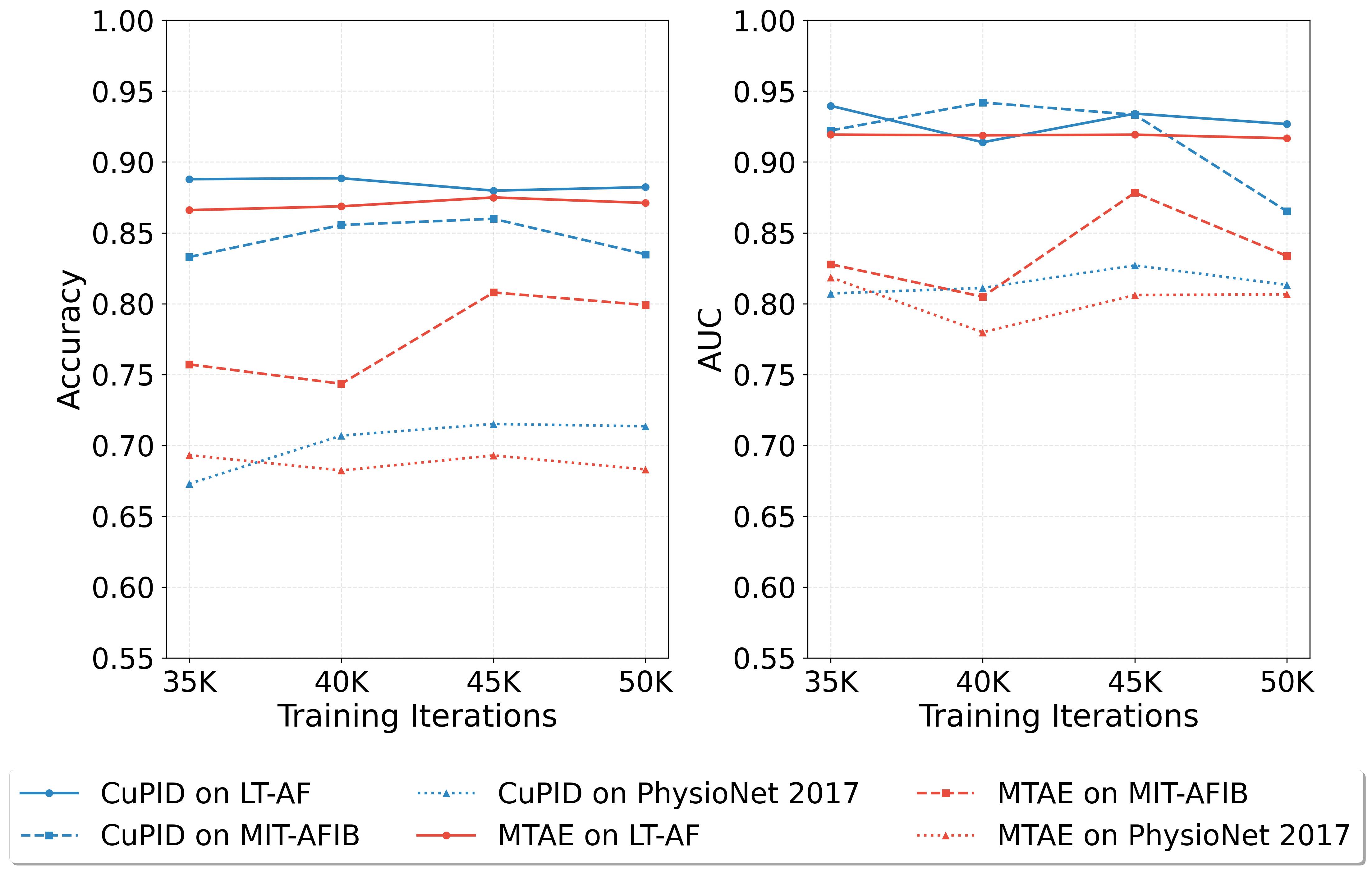
Figure 4: Evolution of the performance over training procedure

Influence of the Model Size:

We evaluated the performance of both models with various encoder sizes. Table 5 indicates that models larger than the proposed one do not show significant improvement. This suggests that an encoder with 4 transformer blocks is adequate to capture the complexity of single-lead ECG signals. Notably, CuPID consistently achieves better results across different datasets and model sizes.

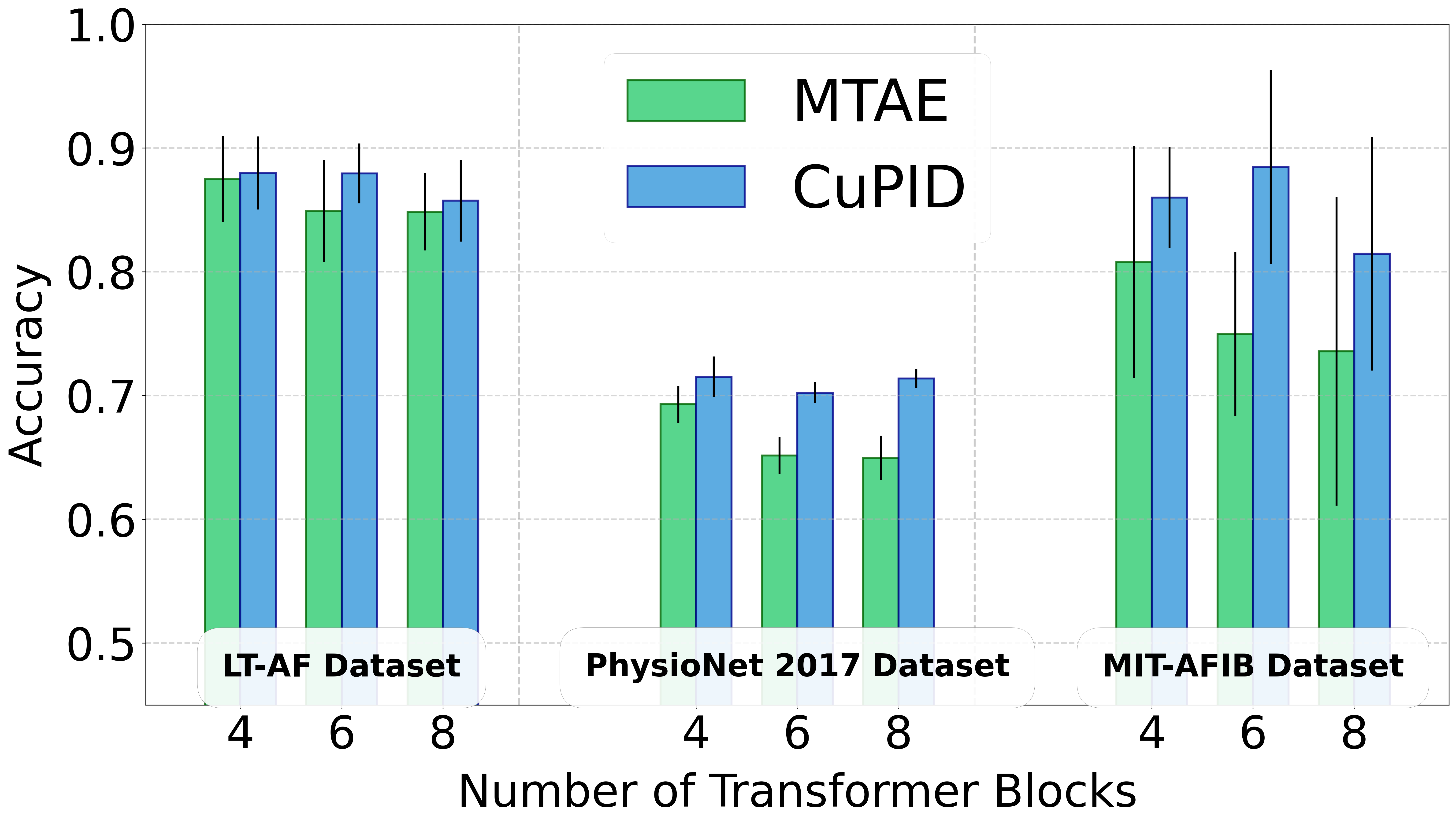
Figure 5: Impact of the model size on the model.

6 Conclusion

This research provides strong evidence that directly applying the Masked Data Modelling (MDM) framework to single-lead ECG signals is suboptimal. Due to the lack of contextual information provided by the unmasked patches of the other leads, the baseline decoder faces challenges when handling irregular heartbeat intervals. This leads the predictor to be cautious when reconstructing the masked patches and to not drive the encoder to compute detailed patch representations that can be used for addressing downstream tasks. To overcome this issue, we introduce CuPID, a novel SSL technique for ECG analysis. By cueing the predictor with the contextual information given by the spectrogram of the input signal, CuPID enforces the encoder to compute more informative representations. It results in a significant performance improvement when addressing downstream tasks.

Limitations:

We have evaluated CuPID solely using one pre-training dataset. As discussed in the manuscript, this is due to SHHS is the only dataset that fits the requirements of all the SSL methods that compose set of baselines.

7 Reproducibility Statement

The attached code as a part of the supplementary material encompasses the implementation of CuPID and several other baselines. Moreover, comprehensive details on training hyperparameters, schemes, and hardware specifications are provided. In addition the pseudocode for the method is provided in the Appendix. Finally, we furnish the pre-trained model’s parameters to facilitate others in achieving reproducible results, together with the code used for processing each database.

Appendix A Data Preprocessing

To ensure the complete reproducibility of this work, this section presents a detailed description of the preprocessing steps employed for the training and evaluation databases utilized in the proposed method.

A.1 SHHS Data Selection

Only the subjects that appear in both recording cycles are used during the training procedure. This leads to 2643 subjects. ECG signals are extracted from the Polysomnography (PSG) recordings. The quality of every 10 seconds-data strips has been evaluated with the algorithm proposed by Zhao and Zhang (Zhao & Zhang, 2018). We use SHHS since it contains two records belonging to the same subject. This makes this specific database special, and this is the reason that it has been the only database used during the optimization.

A.2 Data cleaning

In addition, all signals from the utilized datasets were resampled to a frequency of 100Hz. Then, a $5^{th}$ order Butterworth high-pass filter with a cutoff frequency of 0.5Hz was applied to eliminate any DC-offset and baseline wander. Finally, each dataset underwent normalization to achieve unit variance, ensuring that the signal samples belong to a $\mathcal{N}(0,1)$ distribution. This normalization process aimed to mitigate variations in device amplifications.

Appendix B Details of SHHS Dataset

Table 3: Demographic and Clinical Distribution in the SHHS Dataset

Category	Percentage (%)
Prevalent Atrial Fibrillation (AFib)
No	49.8
Yes	0.8
Unknown	49.4
Race Distribution
White	84.5
Black	8.9
Other	6.6
Age (at Visit 1)	63.1 $\pm$ 11.2 years
Sex Distribution
Male	47.6
Female	52.4

Appendix C Details of Datasets used for Main Evaluation of Single-Lead ECG Baselines

Table 4: Statistics of the PhysioNet 2017 Training Set

Label	Total Recordings	Mean Time (s)	SD Time (s)
Normal	5,154	31.9	10.0
AF	771	31.6	12.5
Other rhythm	2,557	34.1	11.8
Noisy	46	27.1	9.0
Total	8,528	32.5	10.9

Table 5: Statistics of the MIT-BIH Atrial Fibrillation (MIT-AFIB) Database

Label	Total ECGs	Record Count (%)	Avg. ECGs per Record
Normal Sinus Rhythm (NSR)	50,115	21 (91.3%)	0.401 $\pm$ 0.357
Atrial Fibrillation (AFib)	33,694	23 (100%)	0.656 $\pm$ 0.320

Table 6: Statistics of the Long Term AF (LT-AF) Database

Label	Total ECGs	Record Count (%)	Avg. ECGs per Record
Normal Sinus Rhythm (NSR)	270,702	53 (63.1%)	0.672 $\pm$ 0.315
Atrial Fibrillation (AFib)	368,272	84 (100%)	0.546 $\pm$ 0.422
Bradycardia	19,197	35 (41.7%)	0.072 $\pm$ 0.100

C.1 Pseudocode

Algorithm CuPID Training Algorithm

 Input: Number of iterations $K$, Batch size $B$

 Input: Encoder $\mathcal{F}(x)$, Predictor $\mathcal{P}(h,s)$

 Input: Parameters $\theta$, Optimizer $\text{opt}(\theta,\nabla\theta)$

 Input: Spectrogram Transform $S(x)$, Mask Function $\mathcal{RM}(X)$

 Input: Mask Tokens $M_{t}$, Loss Function $\mathcal{L}_{1}(X,Y,M)$

 for $k=0$ to $K$ do

  Sample mini-batch: $X\leftarrow\{X^{1},\dots,X^{N}\}_{b=0}^{B}$

  Apply random masking: $(H_{m},M)\leftarrow\mathcal{RM}(X)$

  Compute encoder representations: $H_{m}\leftarrow\mathcal{F}(H_{m})$

  Attach mask tokens: $H\leftarrow\text{Rec}(H_{m},M_{t})$

  Compute spectrogram: $S\leftarrow S(X)$

  Compute predictor output: $Y\leftarrow\mathcal{P}(H,S)$

  Compute loss: $l\leftarrow\mathcal{L}_{1}(X,Y,M)$

  Compute gradients: $\nabla\theta\leftarrow\frac{\partial l}{\partial\theta}$

  Update parameters: $\theta\leftarrow\text{opt}(\theta,\nabla\theta)$

 end for

Algorithm CuPID Predictor Algorithm

 Input: Predictor Layers $\mathcal{P}$, Final Layer $O(H)$

 Input: Predictor Input $H$, Spectrogram $S$

 for each $(idx,P_{t})$ in $\mathcal{P}$ do

  if $idx=0$ then

   $H\leftarrow P_{t}(H,H,H)$

  else

   $H\leftarrow P_{t}(H,S,H)$ {Feed Spectrogram as Key}

  end if

 end for

 $Y\leftarrow O(H)$

 return $Y$

References

- Abdou & Krishnan (2022) Abdou, A. and Krishnan, S. Horizons in single-lead ecg analysis from devices to data. Frontiers in Signal Processing, 2, 2022. ISSN 2673-8198. doi: 10.3389/frsip.2022.866047. URL https://www.frontiersin.org/articles/10.3389/frsip.2022.866047.
- Assran et al. (2023) Assran, M., Duval, Q., Misra, I., Bojanowski, P., Vincent, P., Rabbat, M., LeCun, Y., and Ballas, N. Self-supervised learning from images with a joint-embedding predictive architecture, 2023. URL https://arxiv.org/abs/2301.08243.
- Atienza et al. (2024) Atienza, A., Bardram, J., and Puthusserypady, S. Contrastive learning is not optimal for quasiperiodic time series. In Larson, K. (ed.), Proceedings of the Thirty-Third International Joint Conference on Artificial Intelligence, IJCAI-24, pp. 3661–3668. International Joint Conferences on Artificial Intelligence Organization, 8 2024. doi: 10.24963/ijcai.2024/405. URL https://doi.org/10.24963/ijcai.2024/405. Main Track.
- Balestriero et al. (2023) Balestriero, R., Ibrahim, M., Sobal, V., Morcos, A., Shekhar, S., Goldstein, T., Bordes, F., Bardes, A., Mialon, G., Tian, Y., Schwarzschild, A., Wilson, A. G., Geiping, J., Garrido, Q., Fernandez, P., Bar, A., Pirsiavash, H., LeCun, Y., and Goldblum, M. A cookbook of self-supervised learning, 2023.
- Bardes et al. (2022) Bardes, A., Ponce, J., and LeCun, Y. Vicreg: Variance-invariance-covariance regularization for self-supervised learning, 2022.
- Bergamaschi et al. (2024) Bergamaschi, T. S., Stultz, C. M., and Alam, R. Heart block identification from 12-lead ecg: Exploring the generalizability of self-supervised ai. In 2024 IEEE 20th International Conference on Body Sensor Networks (BSN), pp. 1–4, 2024. doi: 10.1109/BSN63547.2024.10780740.
- Bing et al. (2022) Bing, P., Liu, Y., Liu, W., Zhou, J., and Zhu, L. Electrocardiogram classification using tsst-based spectrogram and convit. Frontiers in Cardiovascular Medicine, 9, 2022. ISSN 2297-055X. doi: 10.3389/fcvm.2022.983543. URL https://www.frontiersin.org/journals/cardiovascular-medicine/articles/10.3389/fcvm.2022.983543.
- Caron et al. (2021) Caron, M., Touvron, H., Misra, I., Jégou, H., Mairal, J., Bojanowski, P., and Joulin, A. Emerging properties in self-supervised vision transformers, 2021.
- Chen et al. (2020) Chen, T., Kornblith, S., Norouzi, M., and Hinton, G. A simple framework for contrastive learning of visual representations, 2020.
- Clifford et al. (2017) Clifford, G. D., Liu, C., Moody, B., Li-wei, H. L., Silva, I., Li, Q., Johnson, A. E., and Mark, R. G. Af classification from a short single lead ecg recording: The physionet/computing in cardiology challenge 2017. In 2017 Computing in Cardiology (CinC), pp. 1–4. IEEE, Sep 2017. doi: 10.22489/CinC.2017.065-469.
- Devlin et al. (2019) Devlin, J., Chang, M.-W., Lee, K., and Toutanova, K. Bert: Pre-training of deep bidirectional transformers for language understanding, 2019. URL https://arxiv.org/abs/1810.04805.
- Diamant et al. (2022) Diamant, N., Reinertsen, E., Song, S., Aguirre, A. D., Stultz, C. M., and Batra, P. Patient contrastive learning: A performant, expressive, and practical approach to electrocardiogram modeling. PLOS Computational Biology, 18(2):1–16, 02 2022. doi: 10.1371/journal.pcbi.1009862. URL https://doi.org/10.1371/journal.pcbi.1009862.
- Dosovitskiy et al. (2021) Dosovitskiy, A., Beyer, L., Kolesnikov, A., Weissenborn, D., Zhai, X., Unterthiner, T., Dehghani, M., Minderer, M., Heigold, G., Gelly, S., Uszkoreit, J., and Houlsby, N. An image is worth 16x16 words: Transformers for image recognition at scale, 2021.
- Eleyan et al. (2024) Eleyan, A., Bayram, F., and Eleyan, G. Spectrogram-based arrhythmia classification using three-channel deep learning model with feature fusion. Applied Sciences, 14(21):9936, 2024. doi: 10.3390/app14219936.
- Goldberger et al. (2000) Goldberger, A., Amaral, L., Glass, L., Havlin, S., Hausdorg, J., Ivanov, P., Mark, R., Mietus, J., Moody, G., Peng, C.-K., Stanley, H., and Physiobank, P. Components of a new research resource for complex physiologic signals. PhysioNet, 101, 01 2000.
- Grill et al. (2020) Grill, J.-B., Strub, F., Altché, F., Tallec, C., Richemond, P. H., Buchatskaya, E., Doersch, C., Pires, B. A., Guo, Z. D., Azar, M. G., Piot, B., Kavukcuoglu, K., Munos, R., and Valko, M. Bootstrap your own latent: A new approach to self-supervised learning, 2020.
- Guldenring et al. (2022) Guldenring, D., Rababah, A. S., Finlay, D. D., Bond, R. R., Kennedy, A., Doggart, P., and McLaughlin, J. A. D. Influence of the training set size on the subject-to-subject variability of the estimation performance of linear ecg-lead transformations. 2022 Computing in Cardiology (CinC), 498:1–4, 2022. URL https://api.semanticscholar.org/CorpusID:257316995.
- Gupta et al. (2023) Gupta, A., Wu, J., Deng, J., and Fei-Fei, L. Siamese masked autoencoders, 2023.
- He et al. (2021) He, K., Chen, X., Xie, S., Li, Y., Dollár, P., and Girshick, R. Masked autoencoders are scalable vision learners, 2021.
- Himmelreich et al. (2019) Himmelreich, J. C., Karregat, E. P., Lucassen, W. A., van Weert, H. C., de Groot, J. R., Handoko, M. L., Nijveldt, R., and Harskamp, R. E. Diagnostic accuracy of a smartphone-operated, single-lead electrocardiography device for detection of rhythm and conduction abnormalities in primary care. The Annals of Family Medicine, 17(5):403–411, 2019. ISSN 1544-1709. doi: 10.1370/afm.2438. URL https://www.annfammed.org/content/17/5/403.
- Kingma & Ba (2017) Kingma, D. P. and Ba, J. Adam: A method for stochastic optimization, 2017.
- Kiyasseh et al. (2021) Kiyasseh, D., Zhu, T., and Clifton, D. A. Clocs: Contrastive learning of cardiac signals across space, time, and patients, 2021.
- Loshchilov & Hutter (2019) Loshchilov, I. and Hutter, F. Decoupled weight decay regularization, 2019. URL https://arxiv.org/abs/1711.05101.
- Martinez et al. (2004) Martinez, J., Almeida, R., Olmos, S., Rocha, A., and Laguna, P. A wavelet-based ecg delineator: evaluation on standard databases. IEEE Transactions on Biomedical Engineering, 51(4):570–581, 2004. doi: 10.1109/TBME.2003.821031.
- Moody & Mark (1983) Moody, G. and Mark, R. A new method for detecting atrial fibrillation using r-r intervals. Computers in Cardiology, pp. 227–230, 1983.
- Na et al. (2024) Na, Y., Park, M., Tae, Y., and Joo, S. Guiding masked representation learning to capture spatio-temporal relationship of electrocardiogram. In International Conference on Learning Representations, 2024. URL https://openreview.net/forum?id=WcOohbsF4H.
- Petrutiu et al. (2007) Petrutiu, S., Sahakian, A., and Swiryn, S. Abrupt changes in fibrillatory wave charactedstics at the termination of paroxysmal atrial fibrillation in humans. Europace : European pacing, arrhythmias, and cardiac electrophysiology : journal of the working groups on cardiac pacing, arrhythmias, and cardiac cellular electrophysiology of the European Society of Cardiology, 9:466–70, 08 2007. doi: 10.1093/europace/eum096.
- Quan et al. (1998) Quan, S., Howard, B., Iber, C., Kiley, J., Nieto, F., O’Connor, G., Rapoport, D., Redline, S., Robbins, J., Samet, J., and Wahl, P. The sleep heart health study: Design, rationale, and methods. Sleep, 20:1077–85, 01 1998. doi: 10.1093/sleep/20.12.1077.
- Thinh et al. (2022) Thinh, P., Le, D., Brijesh, P., Adjeroh, D., Wu, J., and Jensen, M. Multimodality multi-lead ecg arrhythmia classification using self-supervised learning, 09 2022.
- Vaswani et al. (2017) Vaswani, A., Shazeer, N., Parmar, N., Uszkoreit, J., Jones, L., Gomez, A. N., Kaiser, L. u., and Polosukhin, I. Attention is all you need. In Guyon, I., Luxburg, U. V., Bengio, S., Wallach, H., Fergus, R., Vishwanathan, S., and Garnett, R. (eds.), Advances in Neural Information Processing Systems, volume 30. Curran Associates, Inc., 2017. URL https://proceedings.neurips.cc/paper_files/paper/2017/file/3f5ee243547dee91fbd053c1c4a845aa-Paper.pdf.
- Wickstrøm et al. (2022) Wickstrøm, K., Kampffmeyer, M., Mikalsen, K. Ø., and Jenssen, R. Mixing up contrastive learning: Self-supervised representation learning for time series. Pattern Recognition Letters, 155:54–61, mar 2022. doi: 10.1016/j.patrec.2022.02.007. URL https://doi.org/10.1016%2Fj.patrec.2022.02.007.
- Zhang et al. (2018) Zhang, G.-Q., Cui, L., Mueller, R., Tao, S., Kim, M., Rueschman, M., Mariani, S., Mobley, D., and Redline, S. The national sleep research resource: Towards a sleep data commons. Journal of the American Medical Informatics Association, pp. 572–572, 08 2018. doi: 10.1145/3233547.3233725.
- Zhang et al. (2023) Zhang, H., Liu, W., Shi, J., Chang, S., Wang, H., He, J., and Huang, Q. Maefe: Masked autoencoders family of electrocardiogram for self-supervised pretraining and transfer learning. IEEE Transactions on Instrumentation and Measurement, 72:1–15, 2023. doi: 10.1109/TIM.2022.3228267.
- Zhao & Zhang (2018) Zhao, Z. and Zhang, Y. Sqi quality evaluation mechanism of single-lead ecg signal based on simple heuristic fusion and fuzzy comprehensive evaluation. Frontiers in Physiology, 9, 06 2018. doi: 10.3389/fphys.2018.00727.