The two filter formula reconsidered:
Smoothing in partially observed Gauss–Markov models without information parametrization

Abstract

In this article, the two filter formula is re-examined in the setting of partially observed Gauss–Markov models. It is traditionally formulated as a filter running backward in time, where the Gaussian density is parametrized in “information form”. However, the quantity in the backward recursion is strictly speaking not a distribution, but a likelihood. Taking this observation seriously, a recursion over log-quadratic likelihoods is formulated instead, which obviates the need for “information” parametrization. In particular, it greatly simplifies the square-root formulation of the algorithm. Furthermore, formulae are given for producing the forward Markov representation of the a posteriori distribution over paths from the proposed likelihood representation.

1 Introduction

Consider the following partially observed Markov process

$$x_{0} \sim\pi_{0}(\cdotp)$$ (1a)

$$x_{t}\mid x_{t-1} \sim\pi_{t\mid t-1}(\cdotp\mid x_{t-1})$$ (1b)

$$y_{t}\mid x_{t} \sim h_{t\mid t}(\cdotp\mid x_{t}),$$ (1c)

where $x_{t}$ is the state at time $t$, taking values in $\mathbb{R}^{n}$, and $y_{t}$ is the measurement or observation at time $t$, taking values in $\mathbb{R}^{m}$, with $m\leq n$. Let $t_{i}\leq\bar{t}_{i}$ for $i=1,2,3$, denote their corresponding ranges by $t_{i}\colon\bar{t}_{i}$, and denote the distribution of $x_{t_{2}\mathrel{\mathop{\ordinarycolon}}\bar{t}_{2}}$ conditioned on $x_{t_{1}\mathrel{\mathop{\ordinarycolon}}\bar{t}_{1}}$ and $y_{t_{3}\mathrel{\mathop{\ordinarycolon}}\bar{t}_{3}}$ by

$$\pi^{t_{3}\mathrel{\mathop{\ordinarycolon}}\bar{t}_{3}}_{t_{2}\mathrel{\mathop{\ordinarycolon}}\bar{t}_{2}\mid t_{1}\mathrel{\mathop{\ordinarycolon}}\bar{t}_{1}}(x_{t_{2}\mathrel{\mathop{\ordinarycolon}}\bar{t}_{2}}\mid x_{t_{1}\mathrel{\mathop{\ordinarycolon}}\bar{t}_{1}},y_{t_{3}\mathrel{\mathop{\ordinarycolon}}\bar{t}_{3}}),$$ (2)

where the ranges $t_{1}\mathrel{\mathop{\ordinarycolon}}\bar{t}_{1}$ and $t_{2}\mathrel{\mathop{\ordinarycolon}}\bar{t}_{2}$ are non-overlapping. Similarly, denote the distribution of $y_{t_{2}\mathrel{\mathop{\ordinarycolon}}\bar{t}_{2}}$ conditioned on $x_{t_{1}\mathrel{\mathop{\ordinarycolon}}\bar{t}_{1}}$ and $y_{t_{3}\mathrel{\mathop{\ordinarycolon}}\bar{t}_{3}}$ by

$$h^{t_{3}\mathrel{\mathop{\ordinarycolon}}\bar{t}_{3}}_{t_{2}\mathrel{\mathop{\ordinarycolon}}\bar{t}_{2}\mid t_{1}\mathrel{\mathop{\ordinarycolon}}\bar{t}_{1}}(y_{t_{2}\mathrel{\mathop{\ordinarycolon}}\bar{t}_{2}}\mid x_{t_{1}\mathrel{\mathop{\ordinarycolon}}\bar{t}_{1}},y_{t_{3}\mathrel{\mathop{\ordinarycolon}}\bar{t}_{3}})$$ (3)

where the ranges $t_{1}\mathrel{\mathop{\ordinarycolon}}\bar{t}_{1}$ and $t_{2}\mathrel{\mathop{\ordinarycolon}}\bar{t}_{2}$ are non-overlapping. Lastly, the distribution of $y_{t_{2}\mathrel{\mathop{\ordinarycolon}}\bar{t}_{2}}$ conditioned on $y_{t_{3}\mathrel{\mathop{\ordinarycolon}}\bar{t}_{3}}$ is denoted by

$$L_{t_{2}\mathrel{\mathop{\ordinarycolon}}\bar{t}_{2}\mid t_{3}\mathrel{\mathop{\ordinarycolon}}\bar{t}_{3}}(y_{t_{2}\mathrel{\mathop{\ordinarycolon}}\bar{t}_{2}}\mid y_{t_{3}\mathrel{\mathop{\ordinarycolon}}\bar{t}_{3}}),$$ (4)

where the ranges $t_{1}\mathrel{\mathop{\ordinarycolon}}\bar{t}_{1}$ and $t_{2}\mathrel{\mathop{\ordinarycolon}}\bar{t}_{2}$ are non-overlapping. Given a sequence of measurements $y_{1\mathrel{\mathop{\ordinarycolon}}T}$ the marginal likelihood, $L_{1\mathrel{\mathop{\ordinarycolon}}T}$, and path posterior, $\pi^{1\mathrel{\mathop{\ordinarycolon}}T}_{0\mathrel{\mathop{\ordinarycolon}}T}$, are given by marginalization and Bayes’ rule:

$$L_{1\mathrel{\mathop{\ordinarycolon}}T}(y_{1\mathrel{\mathop{\ordinarycolon}}T}) =\int\pi_{0}(x_{0})\prod_{t=1}^{T}h_{t\mid t}(y_{t}\mid x_{t})\pi_{t\mid t-1}(x_{t}\mid x_{t-1})\operatorname{d\!}x_{0\mathrel{\mathop{\ordinarycolon}}T}$$ (5a)

$$\pi^{1\mathrel{\mathop{\ordinarycolon}}T}_{0\mathrel{\mathop{\ordinarycolon}}T}(x_{0\mathrel{\mathop{\ordinarycolon}}T}\mid y_{1\mathrel{\mathop{\ordinarycolon}}T}) =L_{1\mathrel{\mathop{\ordinarycolon}}T}^{-1}(y_{1\mathrel{\mathop{\ordinarycolon}}T})\pi_{0}(x_{0})\prod_{t=1}^{T}h_{t\mid t}(y_{t}\mid x_{t})\pi_{t\mid t-1}(x_{t}\mid x_{t-1}).$$ (5b)

As the measurement sequence shall be considered fixed it will henceforth be omitted in the expressions (2), (3), (4), and (5). The problem is thus to efficiently compute $L_{1\mathrel{\mathop{\ordinarycolon}}T}$ and interesting quantities from $\pi^{1\mathrel{\mathop{\ordinarycolon}}T}_{0\mathrel{\mathop{\ordinarycolon}}T}$, such as the smoothing distributions, $\pi^{1\mathrel{\mathop{\ordinarycolon}}T}_{t}$, or the a posteriori transition distributions $\pi^{1\mathrel{\mathop{\ordinarycolon}}T}_{t\mid s}$. There are essentially two methods to do this, the forward-backward method (Askar and Derin,, 1981) and backward-forward method (Cappé et al.,, 2005), a catalogue of different forward-backward and backward-forward methods is provided by Ait-El-Fquih and Desbouvries, (2008). The forward-backward method has the advantage that it recursively computes the filtering distributions $\pi^{1\mathrel{\mathop{\ordinarycolon}}t}_{t}$ forward in time; it is thus suitable for on-line inference (Kailath et al.,, 2000, Anderson and Moore,, 2012, Särkkä and Svensson,, 2023). It can also compute the backward transition distributions, $\pi^{1\mathrel{\mathop{\ordinarycolon}}t}_{t\mid t+1}$, from which the smoothing distributions can be computed by the Rauch–Tung–Striebel algorithm (Rauch et al.,, 1965). On the other hand, the backward-forward method computes the likelihoods of the future $h_{t\mathrel{\mathop{\ordinarycolon}}T\mid t-1}$ backward in time. It can also compute the forward transition distributions, $\pi^{t\mathrel{\mathop{\ordinarycolon}}T}_{t\mid t-1}$, from which the smoothing distributions can be computed once $\pi^{1\mathrel{\mathop{\ordinarycolon}}T}_{0}$ has been obtained (see theorem 1 below). Both methods can also be combined to compute the smoothing distributions via the two-filter formula Bresler, (1986)

$$\pi^{1\mathrel{\mathop{\ordinarycolon}}T}_{t}(x)\propto h_{t+1\mathrel{\mathop{\ordinarycolon}}T\mid t}(x)\pi^{1\mathrel{\mathop{\ordinarycolon}}t}_{t}(x)\propto h_{t\mathrel{\mathop{\ordinarycolon}}T\mid t}(x)\pi^{1\mathrel{\mathop{\ordinarycolon}}t-1}_{t}(x)$$ (6)

The two filter formula has been used to construct algorithms for approximate inference in Markovian switching systems (Helmick et al.,, 1995), jump Markov linear systems (Balenzuela et al.,, 2022), navigation problems (Liu et al.,, 2010), and in sequential Monte Carlo (Särkkä et al.,, 2012, Lindsten et al.,, 2013, 2015). The abstract formulae for computing the likelihoods $h_{t\mathrel{\mathop{\ordinarycolon}}T\mid t}$, the a posteriori transition distributions $\pi^{t\mathrel{\mathop{\ordinarycolon}}T}_{t\mid t-1}$, and the marginal likelihood, $L_{1\mathrel{\mathop{\ordinarycolon}}T}$ are given by theorem 1 (Cappé et al.,, 2005, chapter 3).

Theorem 1 (The backward-forward method).

Consider the partially observed Markov process in (1), then $h_{t\mathrel{\mathop{\ordinarycolon}}T\mid t}$ satisfy the following recursion:

$$h_{t\mathrel{\mathop{\ordinarycolon}}T\mid t-1}(x_{t-1}) =\int h_{t\mathrel{\mathop{\ordinarycolon}}T\mid t}(x_{t})\pi_{t\mid t-1}(x_{t}\mid x_{t-1})\operatorname{d\!}x_{t}$$ (7a)

$$h_{t-1\mathrel{\mathop{\ordinarycolon}}T\mid t-1}(x_{t-1}) =h_{t-1\mid t-1}(x_{t-1})h_{t\mathrel{\mathop{\ordinarycolon}}T\mid t-1}(x_{t-1}),$$ (7b)

and the marginal likelihood, $L_{1\mathrel{\mathop{\ordinarycolon}}T}$ is given by

$$L_{1\mathrel{\mathop{\ordinarycolon}}T}=\int h_{1\mathrel{\mathop{\ordinarycolon}}T\mid 0}(x_{0})\pi_{0}(x_{0})\operatorname{d\!}x_{0}.$$ (8)

Additionally, the posterior over paths is given by

$$\pi^{1\mathrel{\mathop{\ordinarycolon}}T}_{0}(x_{0}) =\frac{h_{1\mathrel{\mathop{\ordinarycolon}}T\mid 0}(x_{0})\pi_{0}(x_{0})}{L_{1\mathrel{\mathop{\ordinarycolon}}T}}$$ (9a)

$$\pi^{t\mathrel{\mathop{\ordinarycolon}}T}_{t\mid t-1}(x_{t}\mid x_{t-1}) =\frac{h_{t\mathrel{\mathop{\ordinarycolon}}T\mid t}(x_{t})\pi_{t\mid t-1}(x_{t}\mid x_{t-1})}{h_{t\mathrel{\mathop{\ordinarycolon}}T\mid t-1}(x_{t-1})}$$ (9b)

$$\pi^{1\mathrel{\mathop{\ordinarycolon}}T}_{0\mathrel{\mathop{\ordinarycolon}}T}(x_{0\mathrel{\mathop{\ordinarycolon}}T}) =\pi^{1\mathrel{\mathop{\ordinarycolon}}T}_{0}(x_{0})\Pi_{t=1}^{T}\pi^{t\mathrel{\mathop{\ordinarycolon}}T}_{t\mid t-1}(x_{t}\mid x_{t-1}).$$ (9c)

In this article, the backward-forward algorithm is re-examined when (1) is Gauss–Markov. More specifically, $\pi_{0}$, $\pi_{t\mid t-1}$, and $h_{t\mid t}$ are then given by

$$\pi_{0}(x) =\mathcal{N}(x;\mu_{0},\Sigma_{0})$$ (10a)

$$\pi_{t\mid t-1}(x\mid z) =\mathcal{N}(x;\mu_{t\mid t-1}(z),Q_{t,t-1})$$ (10b)

$$h_{t\mid t}(y\mid x) =\mathcal{N}(y;C_{t}x,R_{t}),$$ (10c)

where the conditional mean function, $\mu_{t\mid t-1}$ is given by

$$\mu_{t\mid t-1}(z)=\Phi_{t,t-1}z+u_{t,t-1}.$$ (11)

The general idea has been around since Mayne, (1966), Fraser and Potter, (1969) and invovles treating $h_{t\mathrel{\mathop{\ordinarycolon}}T\mid t}$ as a distributon and computing it recursively backward in time starting from $h_{T\mid T}$ by what is essentially a Kalman filter (Kalman,, 1961). The method is related to the Lagrange multiplier method for the maximum a posteriori trajectory (Watanabe,, 1985). However, $h_{t\mathrel{\mathop{\ordinarycolon}}T\mid t}$ is not a distribution, and may not be normalizable on $\mathbb{R}^{n}$ (Cappé et al.,, 2005). This problem is circumvented by propagating an information vector, $\xi^{t\mathrel{\mathop{\ordinarycolon}}T}_{t}$, and information matrix, $\Lambda^{t\mathrel{\mathop{\ordinarycolon}}T}_{t}$ instead of a mean vector and covariance matrix (Fraser and Potter,, 1969). The information matrix is related to the covariance matrix by inversion. More specifically, $h_{t\mathrel{\mathop{\ordinarycolon}}T\mid t}$ is parametrized according to (Balenzuela et al.,, 2022)

$$\begin{split}\log h_{t\mathrel{\mathop{\ordinarycolon}}T\mid s}(x)&=\log\mathcal{N}\big{(}x;(\Lambda^{t\mathrel{\mathop{\ordinarycolon}}T}_{t\mid s})^{-1}\xi^{t\mathrel{\mathop{\ordinarycolon}}T}_{t\mid s},(\Lambda^{t\mathrel{\mathop{\ordinarycolon}}T}_{t\mid s})^{-1}\big{)}+\texttt{const}\\ &=-\frac{1}{2}\langle x,\Lambda^{t\mathrel{\mathop{\ordinarycolon}}T}_{t\mid s}x\rangle+\langle\xi^{t\mathrel{\mathop{\ordinarycolon}}T}_{t\mid s},x\rangle+\texttt{const}\end{split}$$ (12)

where the inverse is strictly formal since $\Lambda^{t\mathrel{\mathop{\ordinarycolon}}T}_{t\mid s}$ may not be invertible. As remarked by Balenzuela et al., (2018, 2022), the constant of proportionality, say $\tilde{c}_{t\mid s}$, is often omitted from the computation. This is troublesome in parameter estimation problems as it is required for computing the marginal likelihood, $L_{1\mathrel{\mathop{\ordinarycolon}}T}$ (c.f. theorem 1). The backward recursion for the parametrization (12) is essentially a so-called information filter is run backwards in time (Anderson and Moore,, 2012, sec 6.3). Some formulas in the literature require $\Phi_{t,t-1}$ to be invertible (Kailath et al.,, 2000, section 10.4.2). Other formulas require that $Q_{t,t-1}$ be invertible (Kitagawa,, 2023, section 3.2). These assumptions are restrictive and not even required (Fraser and Potter,, 1969, Särkkä and García-Fernández,, 2020, Balenzuela et al.,, 2018, 2022).

1.1 Contribution

By regarding the backward method as a recursion over likelihoods rather than as a recursion over distributions, an algorithm is obtained which obviates the need for “information” parametrization. More specifically, $h_{t\mathrel{\mathop{\ordinarycolon}}T\mid t}$ is parametrized according to

$$h_{t\mathrel{\mathop{\ordinarycolon}}T\mid t}(x)=c_{t\mathrel{\mathop{\ordinarycolon}}T\mid t}\exp\Big{[}-\frac{1}{2}\mathinner{\lvert\bar{y}_{t\mathrel{\mathop{\ordinarycolon}}T\mid t}-\bar{C}_{t\mathrel{\mathop{\ordinarycolon}}T\mid t}x\rvert}^{2}\Big{]}.$$

This has the consequence that $h_{t\mathrel{\mathop{\ordinarycolon}}T\mid t-1}$ and $\pi^{t\mathrel{\mathop{\ordinarycolon}}T}_{t\mid t-1}$ can be computed by a method that is algebraically equivalent to the classical Kalman update in mean/covariance parametrization. In particular, the author is not aware of anyone giving a method for computing $\pi^{t\mathrel{\mathop{\ordinarycolon}}T}_{t\mid t-1}$ from the backwards recursion. The price to be paid for this convenience is that the formula for computing $h_{t-1\mathrel{\mathop{\ordinarycolon}}T\mid t-1}$ from $h_{t\mathrel{\mathop{\ordinarycolon}}T\mid t-1}$ and $h_{t\mid t}$ is slightly more complicated. More specifically, a QR factorization is required to ensure that the dimensionality $\bar{m}_{t\mid t}$ of $\bar{y}_{t\mathrel{\mathop{\ordinarycolon}}T\mid t}$ does not grow beyond $n$. Additionally, a method only operating on covariance square-roots is developed, assuming that the square-roots $R_{t}^{1/2}$ and $Q_{t,t-1}^{1/2}$ are given.

The remainder of this article is organizes as follows. In section 2 the forward-backward method in the proposed likelihood parametrization is developed, in section 3 this is generalized to only operate on Cholesky factors of covariances, and in section 4 it is shown that the two filter formula becomes algebraically equivalent to the classical Kalman update in the proposed parametrization. Section 5 discusses the interpretation of the likelihood as a density and maximum likelihood estimation of the state based on future measurements. In section 6, the proposed algorithm is demonstrated in a state estimation problem with flat initial distribution, and a concluding discussion is given in section 7.

2 The new backward-forward recursion

In this section, a method for implementing theorem 1 is derived. The novelity lies in that $h_{t\mathrel{\mathop{\ordinarycolon}}T\mid s}$ for $s=t-1,t$ is identified with a linear Gaussian likelihood with identity covariance. Consequently, the likelihood recursion (7) reduces to a recursion over a measurement vector $\bar{y}_{t\mathrel{\mathop{\ordinarycolon}}T\mid s}$ and a measurement matrix $\bar{C}_{t\mathrel{\mathop{\ordinarycolon}}T\mid s}$. The following assumption is not essential to carry out this program, but simplifies the exposition greatly.

Assumption 1.

The measurement covariance matrices $\{R_{t}\}_{t=1}^{T}$ are positive definite.

2.1 The backward recursion

Let $y$ be a vector and $C$ and $R$ matrices of appropriate dimensions. Denote by $\mathcal{Q}(x;y,C,R)$ the following quadratic function:

$$\mathcal{Q}(x;y,C,R)=(y-Cx)^{*}R^{-1}(y-Cx).$$ (13)

When $R$ is the identity matrix, $R=\mathrm{I}$, it is omitted from the notation like so:

$$\mathcal{Q}(x;y,C,\mathrm{I})=\mathcal{Q}(x;y,C).$$ (14)

Note that when $R$ is positive definite then (13) is overparametrized in the sense that $R$ has a unique Cholesky factorization $R=R^{1/2}R^{*/2}$, therefore

$$\begin{split}\mathcal{Q}(x;y,C,R)&=(y-Cx)^{*}R^{-1}(y-Cx)=\mathinner{\lvert R^{-1/2}y-R^{-1/2}Cx\rvert}^{2}\\ &=\mathcal{Q}(x;R^{-1/2}y,R^{-1/2}C).\end{split}$$ (15)

This section is dedicated to proving the following theorem and in the process deriving a recursion for the parameters in (16b) and (16c). The method of proof is by induction.

Theorem 2.

Let assumption 1 be in effect, then $\pi^{t\mathrel{\mathop{\ordinarycolon}}T}_{t\mid t-1}$ and $h_{t\mathrel{\mathop{\ordinarycolon}}T\mid s}$ for $s=t-1,t$ and $t\leq T$ have the following representation:

$$\mu^{t\mathrel{\mathop{\ordinarycolon}}T}_{t\mid t-1}(z) =\Phi^{t\mathrel{\mathop{\ordinarycolon}}T}_{t,t-1}z+u^{t\mathrel{\mathop{\ordinarycolon}}T}_{t,t-1}$$ (16a)

$$\pi^{t\mathrel{\mathop{\ordinarycolon}}T}_{t\mid t-1}(x\mid z) =\mathcal{N}(x;\mu^{t\mathrel{\mathop{\ordinarycolon}}T}_{t\mid t-1}(z),Q^{t\mathrel{\mathop{\ordinarycolon}}T}_{t,t-1})$$ (16b)

$$h_{t\mathrel{\mathop{\ordinarycolon}}T\mid s}(x) =c_{t\mathrel{\mathop{\ordinarycolon}}T\mid s}\exp\Big{[}-\frac{1}{2}\mathcal{Q}(x;\bar{y}_{t\mathrel{\mathop{\ordinarycolon}}T\mid s},\bar{C}_{t\mathrel{\mathop{\ordinarycolon}}T\mid s})\Big{]},$$ (16c)

where $\bar{y}_{t\mathrel{\mathop{\ordinarycolon}}T\mid s}\in\mathbb{R}^{\bar{m}_{t\mathrel{\mathop{\ordinarycolon}}T\mid s}}$ and $\bar{C}_{t\mathrel{\mathop{\ordinarycolon}}T\mid s}\in\mathbb{R}^{\bar{m}_{t\mathrel{\mathop{\ordinarycolon}}T\mid s}\times n}$ and $m\leq\bar{m}_{t\mathrel{\mathop{\ordinarycolon}}T\mid s}\leq n$.

The formula (16c) clearly hold when $T=t=s$, since by assumption 1 and (15)

$$\begin{split}h_{t\mid t}(x)&=\mathcal{N}(y_{t};C_{t}x,R_{t})=\mathinner{\!\left\lvert 2\pi R_{t}\right\rvert}^{-1/2}\exp\Big{[}-\frac{1}{2}\mathcal{Q}(x;y_{t},C_{t},R_{t})\Big{]}\\ &=\mathinner{\!\left\lvert 2\pi R_{t}\right\rvert}^{-1/2}\exp\Big{[}-\frac{1}{2}\mathcal{Q}(x;R_{t}^{-1/2}y_{t},R_{t}^{-1/2}C_{t})\Big{]}=c_{t\mid t}\exp\Big{[}-\frac{1}{2}\mathcal{Q}(x;\bar{y}_{t\mid t},\bar{C}_{t\mid t})\Big{]},\end{split}$$

where the parameters are given by

$$c_{t\mid t} =\mathinner{\!\left\lvert 2\pi R_{t}\right\rvert}^{-1/2},$$ (17a)

$$\bar{y}_{t\mid t} =R_{t}^{-1/2}y_{t},$$ (17b)

$$\bar{C}_{t\mid t} =R_{t}^{-1/2}C_{t}.$$ (17c)

In particular that means that the terminal condition to the the recurrence in theorem 1, $h_{T\mathrel{\mathop{\ordinarycolon}}T\mid T}=h_{T\mid T}$, satisfies (16c). The following proposition shows that (16b) and (16c) hold for $s=t-1$ provided that (16c) hold for $s=t$.

Proposition 1.

Assume that the likelihood, $h_{t\mathrel{\mathop{\ordinarycolon}}T\mid t}$, satisfies (16c), then the likelihood, $h_{t\mathrel{\mathop{\ordinarycolon}}T\mid t-1}$, and the transition distribution, $\pi^{t\mathrel{\mathop{\ordinarycolon}}T}_{t\mid t-1}$, satisfies (16c) and (16b), respectively, with parameters:

$$\hat{R}_{t\mathrel{\mathop{\ordinarycolon}}T\mid t-1} =\mathrm{I}+\bar{C}_{t\mathrel{\mathop{\ordinarycolon}}T\mid t}Q_{t,t-1}\bar{C}_{t\mathrel{\mathop{\ordinarycolon}}T\mid t}^{*},$$ (18a)

$$\bar{y}_{t\mathrel{\mathop{\ordinarycolon}}T\mid t-1} =\hat{R}_{t\mathrel{\mathop{\ordinarycolon}}T\mid t-1}^{-1/2}\big{(}\bar{y}_{t\mathrel{\mathop{\ordinarycolon}}T\mid t}-\bar{C}_{t\mathrel{\mathop{\ordinarycolon}}T\mid t}u_{t,t-1}\big{)}$$ (18b)

$$\bar{C}_{t\mathrel{\mathop{\ordinarycolon}}T\mid t-1} =\hat{R}_{t\mathrel{\mathop{\ordinarycolon}}T\mid t-1}^{-1/2}\bar{C}_{t\mathrel{\mathop{\ordinarycolon}}T\mid t}\Phi_{t,t-1}$$ (18c)

$$\log c_{t\mathrel{\mathop{\ordinarycolon}}T\mid t-1} =\log c_{t\mathrel{\mathop{\ordinarycolon}}T\mid t-1}-\frac{1}{2}\log\mathinner{\lvert\hat{R}_{t\mathrel{\mathop{\ordinarycolon}}T\mid t-1}\rvert}$$ (18d)

$$\bar{K}^{t\mathrel{\mathop{\ordinarycolon}}T}_{t\mid t-1} =Q_{t,t-1}\bar{C}_{t\mathrel{\mathop{\ordinarycolon}}T\mid t}^{*}\hat{R}_{t\mathrel{\mathop{\ordinarycolon}}T\mid t-1}^{-1}$$ (18e)

$$\Phi^{t\mathrel{\mathop{\ordinarycolon}}T}_{t,t-1} =\big{(}\mathrm{I}-\bar{K}^{t\mathrel{\mathop{\ordinarycolon}}T}_{t\mid t-1}\bar{C}_{t\mathrel{\mathop{\ordinarycolon}}T\mid t}\big{)}\Phi_{t,t-1}$$ (18f)

$$u^{t\mathrel{\mathop{\ordinarycolon}}T}_{t,t-1} =u_{t,t-1}+\bar{K}^{t\mathrel{\mathop{\ordinarycolon}}T}_{t\mid t-1}\big{(}\bar{y}_{t\mathrel{\mathop{\ordinarycolon}}T\mid t}-\bar{C}_{t\mathrel{\mathop{\ordinarycolon}}T\mid t}u_{t,t-1}\big{)}$$ (18g)

$$Q^{t\mathrel{\mathop{\ordinarycolon}}T}_{t,t-1} =Q_{t,t-1}-\bar{K}^{t\mathrel{\mathop{\ordinarycolon}}T}_{t\mid t-1}\hat{R}_{t\mathrel{\mathop{\ordinarycolon}}T\mid t-1}(\bar{K}^{t\mathrel{\mathop{\ordinarycolon}}T}_{t\mid t-1})^{*},$$ (18h)

where $\bar{y}_{t\mathrel{\mathop{\ordinarycolon}}T\mid t-1}\in\mathbb{R}^{\bar{m}_{t\mathrel{\mathop{\ordinarycolon}}T\mid t-1}}$, $\bar{C}_{t\mathrel{\mathop{\ordinarycolon}}T\mid s}\in\mathbb{R}^{\bar{m}_{t\mathrel{\mathop{\ordinarycolon}}T\mid t-1}\times n}$, and $\hat{R}_{t\mathrel{\mathop{\ordinarycolon}}T\mid s}\in\mathbb{R}^{\bar{m}_{t\mathrel{\mathop{\ordinarycolon}}T\mid t-1}\times n}$ with

$$\bar{m}_{t\mathrel{\mathop{\ordinarycolon}}T\mid t-1}=\bar{m}_{t\mathrel{\mathop{\ordinarycolon}}T\mid t}.$$ (19)

Proof.

The likelihood, $h_{t\mathrel{\mathop{\ordinarycolon}}T\mid t}$, is by assumption given by

$$h_{t\mathrel{\mathop{\ordinarycolon}}T\mid t}(x)=c_{t\mathrel{\mathop{\ordinarycolon}}T\mid t}\exp\Big{[}-\frac{1}{2}\mathcal{Q}(x;\bar{y}_{t\mathrel{\mathop{\ordinarycolon}}T\mid t},\bar{C}_{t\mathrel{\mathop{\ordinarycolon}}T\mid t})\Big{]}=c_{t\mathrel{\mathop{\ordinarycolon}}T\mid t}(2\pi)^{\bar{m}_{t\mid t}}\mathcal{N}(\bar{y}_{t\mathrel{\mathop{\ordinarycolon}}T\mid t};\bar{C}_{t\mathrel{\mathop{\ordinarycolon}}T\mid t}x,\mathrm{I}).$$

The computation of $h_{t\mathrel{\mathop{\ordinarycolon}}T\mid t-1}$ and $\pi^{t\mathrel{\mathop{\ordinarycolon}}T}_{t\mid t-1}$ is then by by theorem 1, up to a multiplicative constant, equivalent to inference and marginalization in the following model

$$x_{t}\mid x_{t-1} \sim\mathcal{N}(\mu_{t\mid t-1}(x_{t-1}),Q_{t,t-1})$$

$$\bar{y}_{t\mathrel{\mathop{\ordinarycolon}}T\mid t}\mid x_{t},x_{t-1} \sim\mathcal{N}(\bar{y}_{t\mathrel{\mathop{\ordinarycolon}}T\mid t};\bar{C}_{t\mathrel{\mathop{\ordinarycolon}}T\mid t}x_{t},\mathrm{I}),$$

conditionally on $x_{t-1}$. The solution is given by (Särkkä and Svensson,, 2023, c.f. lemma A.2 and A.3)

$$x_{t}\mid x_{t-1},\bar{y}_{t\mathrel{\mathop{\ordinarycolon}}T\mid t} \sim\mathcal{N}(\mu^{t\mathrel{\mathop{\ordinarycolon}}T}_{t\mid t-1}(x_{t-1}),Q^{t\mathrel{\mathop{\ordinarycolon}}T}_{t,t-1})$$

$$\bar{y}_{t\mathrel{\mathop{\ordinarycolon}}T\mid t}\mid x_{t-1} \sim\mathcal{N}\big{(}\bar{C}_{t\mathrel{\mathop{\ordinarycolon}}T\mid t}\big{(}\Phi_{t,t-1}x_{t-1}+u_{t,t-1}\big{)},\hat{R}_{t\mathrel{\mathop{\ordinarycolon}}T\mid t-1}\big{)},$$

with the conditional mean function given by

$$\begin{split}\mu^{t\mathrel{\mathop{\ordinarycolon}}T}_{t\mid t-1}(x)&=\mu_{t\mid t-1}(x)+\bar{K}^{t\mathrel{\mathop{\ordinarycolon}}T}_{t\mid t-1}\big{(}\bar{y}_{t\mathrel{\mathop{\ordinarycolon}}T\mid t}-\bar{C}_{t\mathrel{\mathop{\ordinarycolon}}T\mid t}\mu_{t,t-1}(x)\big{)}\\ &=\Phi^{t\mathrel{\mathop{\ordinarycolon}}T}_{t,t-1}x+u^{t\mathrel{\mathop{\ordinarycolon}}T}_{t,t-1}.\end{split}$$

The last equality is obtained by using (11) and simply matching terms. Furthermore, re-introducing the constant of proportionality gives $h_{t\mathrel{\mathop{\ordinarycolon}}T\mid t-1}$ as

$$\begin{split}h_{t\mathrel{\mathop{\ordinarycolon}}T\mid t-1}(x)&=c_{t\mathrel{\mathop{\ordinarycolon}}T\mid t}(2\pi)^{\bar{m}_{t\mid t}}\mathcal{N}\big{(}\bar{y}_{t\mathrel{\mathop{\ordinarycolon}}T\mid t};\bar{C}_{t\mathrel{\mathop{\ordinarycolon}}T\mid t}\big{(}\Phi_{t,t-1}x+u_{t,t-1}\big{)},\hat{R}_{t\mathrel{\mathop{\ordinarycolon}}T\mid t-1}\big{)}\\ &=c_{t\mathrel{\mathop{\ordinarycolon}}T\mid t}(2\pi)^{\bar{m}_{t\mid t}}\mathcal{N}(\bar{y}_{t\mathrel{\mathop{\ordinarycolon}}T\mid t-1};\bar{C}_{t\mathrel{\mathop{\ordinarycolon}}T\mid t-1}x,\mathrm{I})\\ &=c_{t\mathrel{\mathop{\ordinarycolon}}T\mid t}\mathinner{\lvert\hat{R}_{t\mathrel{\mathop{\ordinarycolon}}T\mid t-1}\rvert}^{-1/2}\exp\Big{[}-\frac{1}{2}\mathcal{Q}(x;\bar{y}_{t\mathrel{\mathop{\ordinarycolon}}T\mid t-1},\bar{C}_{t\mathrel{\mathop{\ordinarycolon}}T\mid t-1})\Big{]},\end{split}$$

which concludes the proof. ∎

With proposition 1 established, it remains to show that if $h_{t\mathrel{\mathop{\ordinarycolon}}T\mid t-1}$ satisfies (16c), then so does $h_{t-1\mathrel{\mathop{\ordinarycolon}}T\mid t-1}$. Under this presupposition, then by theorem 1 and (17), $h_{t-1\mathrel{\mathop{\ordinarycolon}}T\mid t-1}$ is given by

$$\begin{split}h_{t-1\mathrel{\mathop{\ordinarycolon}}T\mid t-1}(x)&=h_{t\mathrel{\mathop{\ordinarycolon}}T\mid t-1}(x)h_{t-1\mid t-1}(x)\\ &=c_{t\mathrel{\mathop{\ordinarycolon}}T\mid t-1}\exp\Big{[}-\frac{1}{2}\mathcal{Q}(x;\bar{y}_{t\mathrel{\mathop{\ordinarycolon}}T\mid t-1},\bar{C}_{t\mathrel{\mathop{\ordinarycolon}}T\mid t-1})\Big{]}\\ &\quad\times c_{t-1\mid t-1}\exp\Big{[}-\frac{1}{2}\mathcal{Q}(x;\bar{y}_{t-1\mid t-1},\bar{C}_{t-1\mid t-1})\Big{]}\end{split}$$ (20)

Now let $\hat{m}_{t-1}=\bar{m}_{t\mathrel{\mathop{\ordinarycolon}}T\mid t-1}+m$ and define $\hat{y}_{t\mathrel{\mathop{\ordinarycolon}}T\mid t-1}\in\mathbb{R}^{\hat{m}_{t-1}}$ and $\hat{C}_{t\mathrel{\mathop{\ordinarycolon}}T\mid t-1}\in\mathbb{R}^{\hat{m}_{t-1}\times n}$ by

$$\hat{y}_{t-1\mathrel{\mathop{\ordinarycolon}}T\mid t-1} =\begin{pmatrix}\bar{y}_{t\mathrel{\mathop{\ordinarycolon}}T\mid t-1}\\ \bar{y}_{t-1\mid t-1}\end{pmatrix}$$ (21a)

$$\hat{C}_{t-1\mathrel{\mathop{\ordinarycolon}}T\mid t-1} =\begin{pmatrix}\bar{C}_{t\mathrel{\mathop{\ordinarycolon}}T\mid t-1}\\ \bar{C}_{t-1\mid t-1}\end{pmatrix},$$ (21b)

then the sum of quadratic functions in (20) evalutes to

$$\mathcal{Q}(x;\bar{y}_{t\mathrel{\mathop{\ordinarycolon}}T\mid t-1},\bar{C}_{t\mathrel{\mathop{\ordinarycolon}}T\mid t-1})+\mathcal{Q}(x;\bar{y}_{t-1\mid t-1},\bar{C}_{t-1\mid t-1})=\mathcal{Q}(x;\hat{y}_{t-1\mathrel{\mathop{\ordinarycolon}}T\mid t-1},\hat{C}_{t-1\mathrel{\mathop{\ordinarycolon}}T\mid t-1}).$$

If $\hat{m}_{t-1}\leq n$ this immediately gives an expression for $h_{t-1\mathrel{\mathop{\ordinarycolon}}T\mid t-1}$ which satisfies the statement of theorem 1. The following proposition summarizes this observation.

Proposition 2.

Assume $h_{t\mathrel{\mathop{\ordinarycolon}}T\mid t-1}$ satisfies (16c) and that $\hat{m}_{t-1}=\bar{m}_{t\mathrel{\mathop{\ordinarycolon}}T\mid t-1}+m\leq n$, then $h_{t-1\mathrel{\mathop{\ordinarycolon}}T\mid t-1}$ satisfies (16c) with parameters

$$\bar{y}_{t-1\mathrel{\mathop{\ordinarycolon}}T\mid t-1} =\hat{y}_{t-1\mathrel{\mathop{\ordinarycolon}}T\mid t-1}$$ (22)

$$\bar{C}_{t-1\mathrel{\mathop{\ordinarycolon}}T\mid t-1} =\hat{C}_{t-1\mathrel{\mathop{\ordinarycolon}}T\mid t-1}$$ (23)

$$c_{t-1\mathrel{\mathop{\ordinarycolon}}T\mid t-1} =c_{t\mathrel{\mathop{\ordinarycolon}}T\mid t-1}c_{t\mid t},$$ (24)

$$m_{t-1\mathrel{\mathop{\ordinarycolon}}T\mid t-1} =\bar{m}_{t\mathrel{\mathop{\ordinarycolon}}T\mid t-1}+m.$$ (25)

The overdetermined case, when $\bar{m}_{t\mathrel{\mathop{\ordinarycolon}}T\mid t-1}+m>n$, requires slightly more effort.

Proposition 3.

Assume $h_{t\mathrel{\mathop{\ordinarycolon}}T\mid t-1}$ satisfies (16c) and $\hat{m}_{t-1}=\bar{m}_{t\mathrel{\mathop{\ordinarycolon}}T\mid t-1}+m>n$. Let $V_{t}U_{t}$ be a QR factorization of $\hat{C}_{t-1\mathrel{\mathop{\ordinarycolon}}T\mid t-1}$ and partition the factors according to

$$\hat{C}_{t-1\mathrel{\mathop{\ordinarycolon}}T\mid t-1}=V_{t}U_{t}=\begin{pmatrix}V_{t,1}&V_{t,2}\end{pmatrix}\begin{pmatrix}\bar{C}_{t-1\mathrel{\mathop{\ordinarycolon}}T\mid t-1}\\ 0_{(\hat{m}_{t-1}-n)\times n}\end{pmatrix},$$ (26)

where $V_{t,1}\in\mathbb{R}^{\hat{m}_{t-1}\times n}$, $V_{t,2}\in\mathbb{R}^{\hat{m}_{t-1}\times(\hat{m}_{t-1}-n)}$, and $\bar{C}_{t-1\mathrel{\mathop{\ordinarycolon}}T\mid t-1}\in\mathbb{R}^{n\times n}$. Furthermore, define $\bar{y}_{t-1\mathrel{\mathop{\ordinarycolon}}T\mid t-1}$ and $e_{t-1}$ by

$$\bar{y}_{t-1\mathrel{\mathop{\ordinarycolon}}T\mid t-1} =V_{t,1}^{*}\hat{y}_{t-1\mathrel{\mathop{\ordinarycolon}}T\mid t-1}$$ (27)

$$e_{t-1} =V_{t,2}^{*}\hat{y}_{t-1\mathrel{\mathop{\ordinarycolon}}T\mid t-1},$$ (28)

then $h_{t-1\mathrel{\mathop{\ordinarycolon}}T\mid t-1}$ satisfies (16c) with remaining parameters given by

$$c_{t-1\mathrel{\mathop{\ordinarycolon}}T\mid t-1} =c_{t\mathrel{\mathop{\ordinarycolon}}T\mid t-1}c_{t\mid t}\exp\Big{[}-\frac{\mathinner{\lvert e_{t-1}\rvert}^{2}}{2}\Big{]}$$ (29)

$$\bar{m}_{t-1\mathrel{\mathop{\ordinarycolon}}T\mid t-1} =n.$$ (30)

Proof.

By assumption and theorem 1, $h_{t-1\mathrel{\mathop{\ordinarycolon}}T\mid t-1}$ is given by

$$\begin{split}h_{t-1\mathrel{\mathop{\ordinarycolon}}T\mid t-1}(x)&=h_{t\mathrel{\mathop{\ordinarycolon}}T\mid t-1}(x)h_{t-1\mid t-1}(x)\\ &=c_{t\mathrel{\mathop{\ordinarycolon}}T\mid t-1}c_{t\mid t}\exp\Big{[}-\frac{1}{2}\mathcal{Q}(x;\hat{y}_{t-1\mathrel{\mathop{\ordinarycolon}}T\mid t-1},\hat{C}_{t-1\mathrel{\mathop{\ordinarycolon}}T\mid t-1})\Big{]}\\ &=c_{t\mathrel{\mathop{\ordinarycolon}}T\mid t-1}c_{t\mid t}\exp\Big{[}-\frac{1}{2}\mathcal{Q}(x;\hat{y}_{t-1\mathrel{\mathop{\ordinarycolon}}T\mid t-1},V_{t}U_{t})\Big{]}\\ &=c_{t\mathrel{\mathop{\ordinarycolon}}T\mid t-1}c_{t\mid t}\exp\Big{[}-\frac{1}{2}\mathcal{Q}(x;V_{t}^{*}\hat{y}_{t-1\mathrel{\mathop{\ordinarycolon}}T\mid t-1},U_{t})\Big{]}\\ &=c_{t\mathrel{\mathop{\ordinarycolon}}T\mid t-1}c_{t\mid t}\exp\Big{[}-\frac{\mathinner{\lvert e_{t-1}\rvert}^{2}}{2}\Big{]}\exp\Big{[}-\frac{1}{2}\mathcal{Q}(x;\bar{y}_{t-1\mathrel{\mathop{\ordinarycolon}}T\mid t-1},\bar{C}_{t-1\mathrel{\mathop{\ordinarycolon}}T\mid t-1})\Big{]},\end{split}$$

which is the desired result. ∎

With propositions 1, 2, and (3) established, theorem 2 hold by induction. It remains to give formulae for the forward recursion. This is done in the following.

2.2 The forward recursion

The previous section established expressions for $\pi^{t\mathrel{\mathop{\ordinarycolon}}T}_{t\mid t-1}$ and $h_{t\mathrel{\mathop{\ordinarycolon}}T\mid s}$ for $s=t-1,t$, the parameters of which are obtained by alternating between proposition 1 and proposition 2 or 3. It remains to compute the a posteriori time marginals, $\{\pi^{1\mathrel{\mathop{\ordinarycolon}}T}_{t}\}_{t=0}^{T}$, and the marginal likelihood, $L_{1\mathrel{\mathop{\ordinarycolon}}T}$. They are all clearly Gaussian and will be denoted by

$$\pi^{1\mathrel{\mathop{\ordinarycolon}}T}_{t}(x)=\mathcal{N}(x;\mu^{1\mathrel{\mathop{\ordinarycolon}}T}_{t},\Sigma^{1\mathrel{\mathop{\ordinarycolon}}T}_{t}),\quad t=0,1,\ldots,T$$ (31)

According to theorem 1, $L_{1\mathrel{\mathop{\ordinarycolon}}T}$ and $\pi^{1\mathrel{\mathop{\ordinarycolon}}T}_{0}$ are simply obtained by Bayes’ rule. By the same argument as in proposition 1, mutatis mutandis, they are given by

$$S_{0} =\bar{C}_{1\mathrel{\mathop{\ordinarycolon}}T\mid 0}\Sigma_{0}\bar{C}_{1\mathrel{\mathop{\ordinarycolon}}T\mid 0}^{*}+\mathrm{I}$$ (32a)

$$K^{1\mathrel{\mathop{\ordinarycolon}}T}_{0} =\Sigma_{0}\bar{C}_{1\mathrel{\mathop{\ordinarycolon}}T\mid 0}^{*}S_{0}^{-1}$$ (32b)

$$\mu^{1\mathrel{\mathop{\ordinarycolon}}T}_{0} =\mu_{0}+K^{1\mathrel{\mathop{\ordinarycolon}}T}_{0}\big{(}\bar{y}_{1\mathrel{\mathop{\ordinarycolon}}T\mid 0}-\bar{C}_{1\mathrel{\mathop{\ordinarycolon}}T\mid 0}\mu_{0}\big{)}$$ (32c)

$$\Sigma^{1\mathrel{\mathop{\ordinarycolon}}T}_{0} =\Sigma_{0}-K^{1\mathrel{\mathop{\ordinarycolon}}T}_{0}S_{0}(K^{1\mathrel{\mathop{\ordinarycolon}}T}_{0})^{*}$$ (32d)

$$L_{1\mathrel{\mathop{\ordinarycolon}}T} =c_{1\mathrel{\mathop{\ordinarycolon}}T\mid 0}(2\pi)^{\bar{m}_{t\mid 0}/2}\mathcal{N}(\bar{y}_{1\mathrel{\mathop{\ordinarycolon}}T\mid 0};\bar{C}_{1\mathrel{\mathop{\ordinarycolon}}T\mid 0}\mu_{0},S_{0})$$ (32e)

Furthermore, the remaining time marginals are then obtained by

$$\mu^{1\mathrel{\mathop{\ordinarycolon}}T}_{t} =\Phi^{t\mathrel{\mathop{\ordinarycolon}}T}_{t,t-1}\mu^{1\mathrel{\mathop{\ordinarycolon}}T}_{t-1}+u^{t\mathrel{\mathop{\ordinarycolon}}T}_{t,t-1}$$ (33a)

$$\Sigma^{1\mathrel{\mathop{\ordinarycolon}}T}_{t} =\Phi^{t\mathrel{\mathop{\ordinarycolon}}T}_{t,t-1}\Sigma^{1\mathrel{\mathop{\ordinarycolon}}T}_{t-1}(\Phi^{t\mathrel{\mathop{\ordinarycolon}}T}_{t,t-1})^{*}+Q^{t\mathrel{\mathop{\ordinarycolon}}T}_{t,t-1}.$$ (33b)

3 The backward-forward recursion in Cholesky form

In order to ensure excellent numerical performance of the algorithm it is preferable to only work with Cholesky factors of the covariance matrices (Kailath et al.,, 2000, section 12). Computing $h_{t-1\mathrel{\mathop{\ordinarycolon}}T\mid t-1}$ from $h_{t-1\mathrel{\mathop{\ordinarycolon}}T\mid t-1}$ and $h_{t-1\mid t-1}$ does not involve any covariances as at all. Hence the only problem in the backward recursion is to compute $h_{t\mathrel{\mathop{\ordinarycolon}}T\mid t-1}$ from $h_{t\mathrel{\mathop{\ordinarycolon}}T\mid t}$ and $\pi_{t\mid t-1}$ without ever forming a covariance matrix. This can be done by so-called array algorithms (Kailath et al.,, 2000, Anderson and Moore,, 2012), the key idea is that for a given matrix $A$ an upper triangular Cholesky factor of $A^{*}A$ may be obtained by the QR decomposition $A=QU$. For an arbitrary matrix $A$, write $A\cong U$ when $U$ is the upper triangular factor in the QR factorization of $A$.

Proposition 4.

Consider the same setting as propositon 1, then

$$\begin{pmatrix}\mathrm{I}&0\\ Q_{t,t-1}^{*/2}\bar{C}_{t\mathrel{\mathop{\ordinarycolon}}T\mid t}^{*}&Q_{t,t-1}^{*/2}\end{pmatrix}\cong\begin{pmatrix}\hat{R}_{t\mathrel{\mathop{\ordinarycolon}}T\mid t-1}^{*/2}&(\hat{K}^{t\mathrel{\mathop{\ordinarycolon}}T}_{t\mid t-1})^{*}\\ 0&(Q_{t,t-1}^{t\mathrel{\mathop{\ordinarycolon}}T})^{*/2}\end{pmatrix},$$ (34)

where $\hat{K}^{t\mathrel{\mathop{\ordinarycolon}}T}_{t\mid t-1}$ is related to $\bar{K}^{t\mathrel{\mathop{\ordinarycolon}}T}_{t\mid t-1}$ by

$$\bar{K}^{t\mathrel{\mathop{\ordinarycolon}}T}_{t\mid t-1}=\hat{K}^{t\mathrel{\mathop{\ordinarycolon}}T}_{t\mid t-1}\hat{R}_{t\mathrel{\mathop{\ordinarycolon}}T\mid t-1}^{-1/2},$$ (35)

and the parameters of $h_{t\mathrel{\mathop{\ordinarycolon}}T\mid t-1}$ are given by

$$\bar{y}_{t\mathrel{\mathop{\ordinarycolon}}T\mid t-1} =\hat{R}_{t\mathrel{\mathop{\ordinarycolon}}T\mid t-1}^{-1/2}\big{(}\bar{y}_{t\mathrel{\mathop{\ordinarycolon}}T\mid t}-\bar{C}_{t\mathrel{\mathop{\ordinarycolon}}T\mid t}u_{t,t-1}\big{)}$$ (36)

$$\bar{C}_{t\mathrel{\mathop{\ordinarycolon}}T\mid t-1} =\hat{R}_{t\mathrel{\mathop{\ordinarycolon}}T\mid t-1}^{-1/2}\bar{C}_{t\mathrel{\mathop{\ordinarycolon}}T\mid t}\Phi_{t,t-1}$$ (37)

$$\log c_{t\mathrel{\mathop{\ordinarycolon}}T\mid t-1} =\log c_{t\mathrel{\mathop{\ordinarycolon}}T\mid t-1}-\log\mathinner{\lvert\hat{R}_{t\mathrel{\mathop{\ordinarycolon}}T\mid t-1}^{1/2}\rvert}.$$ (38)

Furthermore, the remaining parameters of $\pi^{t\mathrel{\mathop{\ordinarycolon}}T}_{t\mid t-1}$ are given by

$$\Phi^{t\mathrel{\mathop{\ordinarycolon}}T}_{t,t-1} =\Phi_{t,t-1}-\hat{K}^{t\mathrel{\mathop{\ordinarycolon}}T}_{t\mid t-1}\bar{C}_{t\mathrel{\mathop{\ordinarycolon}}T\mid t-1}$$ (39)

$$u^{t\mathrel{\mathop{\ordinarycolon}}T}_{t,t-1} =u_{t,t-1}+\hat{K}^{t\mathrel{\mathop{\ordinarycolon}}T}_{t\mid t-1}\bar{y}_{t\mathrel{\mathop{\ordinarycolon}}T\mid t-1}.$$ (40)

Remark 1.

Pay attention to the time index of $\bar{y}$ and $\bar{C}$ in the expressions for $\Phi^{t\mathrel{\mathop{\ordinarycolon}}T}_{t,t-1}$ and $u^{t\mathrel{\mathop{\ordinarycolon}}T}_{t,t-1}$ in proposition 4. It differs from the corresponding expression in proposition 1.

Proof.

The identities (34) and (35) are known (Anderson and Moore,, 2012, section 6.5). The proof concludes by inserting these into the relations given by proposition 1 and identifying terms. ∎

The parameters of the initial distribution are obtained by the same argument as proposition 4. More specifically, substitue $Q_{t,t-1}$ and $\bar{C}_{t\mathrel{\mathop{\ordinarycolon}}T\mid t}$ on the left-hand side of (34) with $\Sigma_{0}$ and $\bar{C}_{1\mathrel{\mathop{\ordinarycolon}}T\mid 0}$ to obtain $S_{0}^{1/2}$, $\hat{K}_{0}^{1\mathrel{\mathop{\ordinarycolon}}T}$, and $(\Sigma^{1\mathrel{\mathop{\ordinarycolon}}T}_{0})^{*/2}$ as the right-hand side of (34). The remaining parameter, $\mu^{1\mathrel{\mathop{\ordinarycolon}}T}_{0}$, is then obtained by using the relation between $\hat{K}_{0}^{1\mathrel{\mathop{\ordinarycolon}}T}$ and $K_{0}^{1\mathrel{\mathop{\ordinarycolon}}T}$ corresponding to (35) and substitution into (32)

$$\mu^{1\mathrel{\mathop{\ordinarycolon}}T}_{0}=\mu_{0}+\hat{K}_{0}^{1\mathrel{\mathop{\ordinarycolon}}T}S_{0}^{-1/2}\big{(}\bar{y}_{1\mathrel{\mathop{\ordinarycolon}}T\mid 0}-\bar{C}_{1\mathrel{\mathop{\ordinarycolon}}T\mid 0}\mu_{0}\big{)}.$$ (41)

Furthermore, the mean of the smoothing marginals is still obtained by (33), while the Cholesky factor of the covariances clearly satisifes the following recursion:

$$\begin{pmatrix}\Phi^{t\mathrel{\mathop{\ordinarycolon}}T}_{t,t-1}(\Sigma^{1\mathrel{\mathop{\ordinarycolon}}T}_{t-1})^{1/2}&(Q^{t\mathrel{\mathop{\ordinarycolon}}T}_{t,t-1})^{1/2}\end{pmatrix}^{*}\cong(\Sigma^{1\mathrel{\mathop{\ordinarycolon}}T}_{t})^{*/2}.$$ (42)

That is, $(\Sigma^{1\mathrel{\mathop{\ordinarycolon}}T}_{t})^{*/2}$ is the upper triangular factor i the QR factorization of the left-hand side of the preceeding expression.

4 The two-filter formula

Assume the filtering densities $\pi^{1\mathrel{\mathop{\ordinarycolon}}t}_{t}$ have been obtained, by for example running a standard Kalman filter (Särkkä and Svensson,, 2023) or a square-root variant (Anderson and Moore,, 2012, section 6.5), then they are given by

$$\pi^{1\mathrel{\mathop{\ordinarycolon}}t}_{t}(x)=\mathcal{N}(x;\mu_{t}^{1\mathrel{\mathop{\ordinarycolon}}t},\Sigma^{1\mathrel{\mathop{\ordinarycolon}}t}_{t}).$$ (43)

Furthermore, by theorem 2, the two-filter formula (6) reduces to

$$\pi^{1\mathrel{\mathop{\ordinarycolon}}T}_{t}(x)\propto h_{t+1\mathrel{\mathop{\ordinarycolon}}T\mid t}(x)\pi^{1\mathrel{\mathop{\ordinarycolon}}t}_{t}(x)\propto\mathcal{N}(\bar{y}_{t+1\mathrel{\mathop{\ordinarycolon}}T\mid t};\bar{C}_{t+1\mathrel{\mathop{\ordinarycolon}}T\mid t}x,\mathrm{I})\mathcal{N}(x;\mu^{1\mathrel{\mathop{\ordinarycolon}}t}_{t},\Sigma^{1\mathrel{\mathop{\ordinarycolon}}t}_{t}).$$ (44)

This is equivalent to obtaining the posterior in the following model,

$$x_{t} \sim\mathcal{N}(\mu^{1\mathrel{\mathop{\ordinarycolon}}t}_{t},\Sigma^{1\mathrel{\mathop{\ordinarycolon}}t}_{t}),$$ (45)

$$\bar{y}_{t+1\mathrel{\mathop{\ordinarycolon}}T\mid t}\mid x_{t} \sim\mathcal{N}(\bar{y}_{t+1\mathrel{\mathop{\ordinarycolon}}T\mid t};\bar{C}_{t+1\mathrel{\mathop{\ordinarycolon}}T\mid t}x_{t},\mathrm{I}),$$ (46)

hence the mean, $\mu^{1\mathrel{\mathop{\ordinarycolon}}T}_{t}$ and covariance, $\Sigma^{1\mathrel{\mathop{\ordinarycolon}}T}_{t}$, of $\pi^{1\mathrel{\mathop{\ordinarycolon}}t}_{t}$ can be obtained by a classical Kalman update or its’ square-root variant. (Anderson and Moore,, 2012).

5 Relationship to information parametrization, maximum likelihood estimation, and the likelihood as a density

The purpose of this section is to relate the present parametrization of $h_{t\mathrel{\mathop{\ordinarycolon}}T\mid s}$ with the information parametrization and to clarify its interpretation as a density. From the preceeding discussion, the likelihood $h_{t\mathrel{\mathop{\ordinarycolon}}T\mid s}$ for $s=t-1,t$ is given by

$$h_{t\mathrel{\mathop{\ordinarycolon}}T\mid s}(x)=c_{1\mathrel{\mathop{\ordinarycolon}}T\mid s}\exp\Big{[}-\frac{1}{2}\mathcal{Q}(x;\bar{y}_{t\mathrel{\mathop{\ordinarycolon}}T\mid s},\bar{C}_{t\mathrel{\mathop{\ordinarycolon}}T\mid s})\Big{]}.$$ (47)

The quadratic form above is given by

$$\mathcal{Q}(x;\bar{y}_{t\mathrel{\mathop{\ordinarycolon}}T\mid s},\bar{C}_{t\mathrel{\mathop{\ordinarycolon}}T\mid s})=\langle x,\bar{C}_{t\mathrel{\mathop{\ordinarycolon}}T\mid s}^{*}\bar{C}_{t\mathrel{\mathop{\ordinarycolon}}T\mid s}x\rangle-2\langle\bar{C}_{t\mathrel{\mathop{\ordinarycolon}}T\mid s}^{*}\bar{y}_{t\mathrel{\mathop{\ordinarycolon}}T\mid s},x\rangle+\mathtt{const}.$$ (48)

The correspondence to the information parametrization is then (c.f. (12))

$$\xi^{t\mathrel{\mathop{\ordinarycolon}}T}_{s} =\bar{C}_{t\mathrel{\mathop{\ordinarycolon}}T\mid s}^{*}\bar{y}_{t\mathrel{\mathop{\ordinarycolon}}T\mid s},$$ (49a)

$$\Lambda^{t\mathrel{\mathop{\ordinarycolon}}T}_{s} =\bar{C}_{t\mathrel{\mathop{\ordinarycolon}}T\mid s}^{*}\bar{C}_{t\mathrel{\mathop{\ordinarycolon}}T\mid s}.$$ (49b)

Hence, $\bar{C}_{t\mathrel{\mathop{\ordinarycolon}}T\mid s}$ may be viewed as a $\bar{m}_{t\mid s}\times n$ square-root of $\Lambda^{t\mathrel{\mathop{\ordinarycolon}}T}_{s}$. The relationship between $\xi^{t\mathrel{\mathop{\ordinarycolon}}T}_{s}$ and $\bar{y}_{t\mathrel{\mathop{\ordinarycolon}}T\mid s}$ is a bit more opaque and perhaps best understood in terms of the mean/covariance parametrization. Let $\mu^{t\mathrel{\mathop{\ordinarycolon}}T}_{s}$ be the minimum norm solution to the following equation

$$0=\nabla\log h_{t\mathrel{\mathop{\ordinarycolon}}T\mid s}(x)=\bar{C}_{t\mathrel{\mathop{\ordinarycolon}}T\mid s}^{*}(\bar{y}_{t\mathrel{\mathop{\ordinarycolon}}T\mid s}-\bar{C}_{t\mathrel{\mathop{\ordinarycolon}}T\mid s}x),$$ (50)

then $\mu^{t\mathrel{\mathop{\ordinarycolon}}T}_{s}$ is the maximum likelihood estimate of $x_{s}$ based on data $y_{t\mathrel{\mathop{\ordinarycolon}}T}$ of smallest norm. Now define $\Sigma^{t\mathrel{\mathop{\ordinarycolon}}T}_{s}$ by

$$\Sigma^{t\mathrel{\mathop{\ordinarycolon}}T}_{s}=(\Lambda^{t\mathrel{\mathop{\ordinarycolon}}T}_{s})^{+}=(\bar{C}_{t\mathrel{\mathop{\ordinarycolon}}T\mid s}^{*}\bar{C}_{t\mathrel{\mathop{\ordinarycolon}}T\mid s})^{+}=\bar{C}_{t\mathrel{\mathop{\ordinarycolon}}T\mid s}^{+}(\bar{C}_{t\mathrel{\mathop{\ordinarycolon}}T\mid s}^{*})^{+}$$ (51)

where ⁺ denotes a generalized matrix inverse and the last equality is taken known from e.g. Greville, (1966). An explicit expression of $\mu^{t\mathrel{\mathop{\ordinarycolon}}T}_{s}$ is then given by

$$\mu^{t\mathrel{\mathop{\ordinarycolon}}T}_{s}=\Sigma^{t\mathrel{\mathop{\ordinarycolon}}T}_{s}\bar{C}_{t\mathrel{\mathop{\ordinarycolon}}T\mid s}^{*}\bar{y}_{t\mathrel{\mathop{\ordinarycolon}}T\mid s}=\bar{C}_{t\mathrel{\mathop{\ordinarycolon}}T\mid s}^{+}(\bar{C}_{t\mathrel{\mathop{\ordinarycolon}}T\mid s}^{*})^{+}\bar{C}_{t\mathrel{\mathop{\ordinarycolon}}T\mid s}^{*}\bar{y}_{t\mathrel{\mathop{\ordinarycolon}}T\mid s}=(\Sigma^{t\mathrel{\mathop{\ordinarycolon}}T}_{s})^{1/2}(\bar{C}_{t\mathrel{\mathop{\ordinarycolon}}T\mid s}^{*})^{+}\bar{C}_{t\mathrel{\mathop{\ordinarycolon}}T\mid s}^{*}\bar{y}_{t\mathrel{\mathop{\ordinarycolon}}T\mid s}.$$ (52)

The observation vector $\bar{y}_{t\mathrel{\mathop{\ordinarycolon}}T\mid s}$ has identity covariance conditioned on $x_{s}$ (by construction), hence the conditional covariance of $\mu^{t\mathrel{\mathop{\ordinarycolon}}T}_{s}$ is given by

$$\Sigma^{t\mathrel{\mathop{\ordinarycolon}}T}_{s}\bar{C}_{t\mathrel{\mathop{\ordinarycolon}}T\mid s}^{*}\bar{C}_{t\mathrel{\mathop{\ordinarycolon}}T\mid s}\Sigma^{t\mathrel{\mathop{\ordinarycolon}}T}_{s}=(\Lambda^{t\mathrel{\mathop{\ordinarycolon}}T}_{s})^{+}\Lambda^{t\mathrel{\mathop{\ordinarycolon}}T}_{s}(\Lambda^{t\mathrel{\mathop{\ordinarycolon}}T}_{s})^{+}=(\Lambda^{t\mathrel{\mathop{\ordinarycolon}}T}_{s})^{+}=\Sigma^{t\mathrel{\mathop{\ordinarycolon}}T}_{s},$$ (53)

which justifies the notation $\Sigma^{t\mathrel{\mathop{\ordinarycolon}}T}_{s}$ for $(\Lambda^{t\mathrel{\mathop{\ordinarycolon}}T}_{s})^{+}$. In view of (52), the observation vector $\bar{y}_{t\mathrel{\mathop{\ordinarycolon}}T\mid s}$ may then be interpreted as a the mean vector $\mu^{t\mathrel{\mathop{\ordinarycolon}}T}_{s}$ “whitened” by $\Sigma^{t\mathrel{\mathop{\ordinarycolon}}T}_{s}$.

It is now tempting to interpret $h_{t\mathrel{\mathop{\ordinarycolon}}T\mid s}$ as an unnormalized Gaussian density with mean $\mu^{t\mathrel{\mathop{\ordinarycolon}}T}_{s}$ and covariance $\Sigma^{t\mathrel{\mathop{\ordinarycolon}}T}_{s}$. This can indeed be done, but the density will not not be supported on the whole of $\mathbb{R}^{n}$ but rather on an affine subset, $\Omega_{t\mathrel{\mathop{\ordinarycolon}}T\mid s}$, which is given by (Rao,, 1973, Chapter 8)

$$\Omega_{t\mathrel{\mathop{\ordinarycolon}}T\mid s}=\big{\{}x\colon x=\mu^{t\mathrel{\mathop{\ordinarycolon}}T}_{s}+v,\quad v\in\operatorname{range}\Sigma^{t\mathrel{\mathop{\ordinarycolon}}T}_{s}\big{\}}.$$ (54)

The integral of $h_{t\mathrel{\mathop{\ordinarycolon}}T\mid s}$ over $\Omega_{t\mathrel{\mathop{\ordinarycolon}}T\mid s}$ is then given by

$$\begin{split}\int_{\Omega_{t\mathrel{\mathop{\ordinarycolon}}T\mid s}}h_{t\mathrel{\mathop{\ordinarycolon}}T\mid s}(x)\operatorname{d\!}x&=c_{1\mathrel{\mathop{\ordinarycolon}}T\mid s}\int_{\Omega_{t\mid s}}\exp\Big{[}-\frac{1}{2}(x-\mu^{t\mathrel{\mathop{\ordinarycolon}}T}_{s})^{*}(\Sigma^{t\mathrel{\mathop{\ordinarycolon}}T}_{s})^{+}(x-\mu^{t\mathrel{\mathop{\ordinarycolon}}T}_{s})\Big{]}\operatorname{d\!}x\\ &=c_{1\mathrel{\mathop{\ordinarycolon}}T\mid s}\mathinner{\lvert 2\pi\Sigma^{t\mathrel{\mathop{\ordinarycolon}}T}_{s}\rvert}^{1/2}_{+},\end{split}$$ (55)

where $\mathinner{\!\left\lvert\cdotp\right\rvert}_{+}$ denotes the product of all non-zero eigenvalues, the so-called pseudo-determinant. The notation $\operatorname{d\!}x$ is here overloaded to also mean the Lebesgue measure on $\Omega_{t\mathrel{\mathop{\ordinarycolon}}T\mid s}$. Thus the inference problem can be solved even when $\pi_{0}$ is flat (improper) on $\Omega_{t\mid s}$. In particular, the following result is obtained by the preceeding discussion.

Proposition 5.

Let the a priori initial distribution be given by

$$\pi_{0}(x)=\chi_{\Omega_{1\mathrel{\mathop{\ordinarycolon}}T\mid 0}}(x),$$ (56)

where $\chi_{A}$ is the indicator function on the set $A$. Then the marginal likelihood, $L_{1\mathrel{\mathop{\ordinarycolon}}T}$, and the a posteriori initial density, $\pi^{1\mathrel{\mathop{\ordinarycolon}}T}_{0}$, are given by

$$L_{1\mathrel{\mathop{\ordinarycolon}}T} =c_{1\mathrel{\mathop{\ordinarycolon}}T\mid 0}\mathinner{\lvert 2\pi\Sigma^{t\mathrel{\mathop{\ordinarycolon}}T}_{0}\rvert}^{1/2}_{+}$$ (57a)

$$\pi^{1\mathrel{\mathop{\ordinarycolon}}T}_{0}(x) =\begin{cases}\mathcal{N}(x;\mu^{t\mathrel{\mathop{\ordinarycolon}}T}_{0},\Sigma^{t\mathrel{\mathop{\ordinarycolon}}T}_{0}),\quad x\in\Omega_{1\mathrel{\mathop{\ordinarycolon}}T\mid 0}\\ 0,\quad x\in\Omega_{1\mathrel{\mathop{\ordinarycolon}}T\mid 0}^{\mathsf{c}}\end{cases}.$$ (57b)

Note that $\pi_{0}^{1\mathrel{\mathop{\ordinarycolon}}T}$ can still be obtained by similar means as in proposition 5 when $\pi_{0}$ is flat on all of $\mathbb{R}^{n}$. The difference being that $\pi^{1\mathrel{\mathop{\ordinarycolon}}T}_{0}$ will remain flat on $\Omega_{1\mathrel{\mathop{\ordinarycolon}}T\mid 0}^{\mathsf{c}}$ rather than being unsupported. However, the marginal likelihood, $L_{1\mathrel{\mathop{\ordinarycolon}}T}$, will be infinite. Therefore, in such a siutation it is perhaps more appropriate to treat $x_{0}$ as a parameter in which case the marginal likelihood may identified with $h_{1\mathrel{\mathop{\ordinarycolon}}T\mid 0}$.

6 An example of unknown origin

Consider an object moving in the plane and denote its position at time $\tau$ by $p(\tau)$. Let the dynamics of the object be governed by the following continuous-time model

$$\operatorname{d\!}\ddot{p}(\tau)=\begin{pmatrix}\sigma_{1}&0\\ 0&\sigma_{2}\end{pmatrix}\operatorname{d\!}w(\tau),\quad\tau\geq 0,$$ (58)

where $\ddot{p}$ is the acceleration and $w$ is a two dimensional standard Wiener process. Starting at time $\tau=127$, the position of the object is measured at every time unit up until $\tau=256$ according to

$$y(\tau_{k})=p(\tau_{k})+\begin{pmatrix}\sqrt{\lambda_{1}}&0\\ 0&\sqrt{\lambda_{2}}\end{pmatrix}v(\tau_{k}),$$ (59)

where $v(\tau_{k})$ is a sequence of two dimensional independent standard Gaussian vectors, $\tau_{k}=k$. Collecting the acceleration, $\ddot{p}(\tau)$, the velocity, $\dot{p}(\tau)$, and the position, $p(\tau)$, into a state vector $x(\tau)$ gives a continuous-discrete stochastic state-space model representation of (58) and (59). Furthermore, by discretizing the continuous-time process and setting $x_{k}=x(\tau_{k})$ and taking $x_{0}$ as completely unknown gives the following discrete-time model:

$$x_{0} \sim\chi_{\mathbb{R}^{6}}(\cdotp)$$ (60a)

$$x_{k}\mid x_{k-1} \sim\mathcal{N}(\Phi x_{k-1},Q),\quad k=1,2,\ldots,256,$$ (60b)

$$y_{k}\mid x_{k} \sim\mathcal{N}(Cx_{k},R),\quad k=127,128,\ldots,256.$$ (60c)

The problem is to determine the position, $p(\tau_{k})$, of the object for $k=0,1,\ldots,126$, that is at times before the measurement process started.

Two options based on the backward-forward method are considered:

1. The complete forward-backward algorithm using proposition 5 to compute $\pi_{0}^{127\mathrel{\mathop{\ordinarycolon}}256}$

2. Computing the maximum likelihood estiamte of $x_{k}$ by maximizing $h_{127\mathrel{\mathop{\ordinarycolon}}256\mid k}$.

The results are shown in figures 1 and 2, respectively. As expected, the estimation quality of running the complete forward-backward algorithm is better than just doing maximum likelihood estimation.

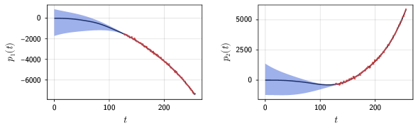
Figure 1: The position of the object (black), the position observations (red), and a $\pm 2\sigma$ credible interval of the position (blue). The estimate was obtained by the forward-backward algorithm.

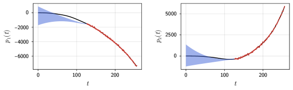
Figure 2: The position of the object (black), the position observations (red), and a $\pm 2\sigma$ confidence interval of the position (blue). The estimate was obtained by maximum likelihood.

7 Discussion

This article presents a new backward-forward method was developed for inference in partially observed Gauss–Markov models. The benefit is that all computations are carried out with respect to the covariance parametrization or its’ square-root variant. Furthermore, simple expressions for the forward a posteriori transition distributions, $\pi^{t\mathrel{\mathop{\ordinarycolon}}T}_{t\mid t-1}$, were obtained. This in turn gives a forward Markov representation of the path posterior, $\pi^{1\mathrel{\mathop{\ordinarycolon}}T}_{0\mathrel{\mathop{\ordinarycolon}}T}$, which may be simpler to work with in certain applications such as parameter estimation using variational methods.

References

• Ait-El-Fquih and Desbouvries, (2008) Ait-El-Fquih, B. and Desbouvries, F. (2008). On Bayesian fixed-interval smoothing algorithms. IEEE Transactions on Automatic Control, 53(10):2437–2442.
• Anderson and Moore, (2012) Anderson, B. D. O. and Moore, J. B. (2012). Optimal filtering. Courier Corporation.
• Askar and Derin, (1981) Askar, M. and Derin, H. (1981). A recursive algorithm for the Bayes solution of the smoothing problem. IEEE Transactions on Automatic Control, 26(2):558–561.
• Balenzuela et al., (2018) Balenzuela, M. P., Dahlin, J., Bartlett, N., Wills, A. G., Renton, C., and Ninness, B. (2018). Accurate Gaussian mixture model smoothing using a two-filter approach. In 2018 IEEE Conference on Decision and Control (CDC), pages 694–699. IEEE.
• Balenzuela et al., (2022) Balenzuela, M. P., Wills, A. G., Renton, C., and Ninness, B. (2022). A new smoothing algorithm for jump Markov linear systems. Automatica, 140:110218.
• Bresler, (1986) Bresler, Y. (1986). Two-filter formulae for discrete-time non-linear Bayesian smoothing. International Journal of Control, 43(2):629–641.
• Cappé et al., (2005) Cappé, O., Moulines, E., and Rydén, T. (2005). Inference in Hidden Markov Models. Springer.
• Fraser and Potter, (1969) Fraser, D. and Potter, J. (1969). The optimum linear smoother as a combination of two optimum linear filters. IEEE Transactions on Automatic Control, 14(4):387–390.
• Greville, (1966) Greville, T. N. E. (1966). Note on the generalized inverse of a matrix product. SIAM Review, 8(4):518–521.
• Helmick et al., (1995) Helmick, R. E., Blair, W. D., and Hoffman, S. A. (1995). Fixed-interval smoothing for Markovian switching systems. IEEE Transactions on Information Theory, 41(6):1845–1855.
• Kailath et al., (2000) Kailath, T., Sayed, A. H., and Hassibi, B. (2000). Linear estimation. Prentice Hall.
• Kalman, (1961) Kalman, R. E. (1961). New results in linear filtering and prediction theory. Transactions of the ASME, Journal of Basic Engineering, 82:35–45.
• Kitagawa, (2023) Kitagawa, G. (2023). Revisiting the two-filter formula for smoothing for state-space models. arXiv preprint arXiv:2307.03428.
• Lindsten et al., (2013) Lindsten, F., Bunch, P., Godsill, S. J., and Schön, T. B. (2013). Rao-Blackwellized particle smoothers for mixed linear/nonlinear state-space models. In 2013 IEEE International Conference on Acoustics, Speech and Signal Processing, pages 6288–6292. IEEE.
• Lindsten et al., (2015) Lindsten, F., Bunch, P., Särkkä, S., Schön, T. B., and Godsill, S. J. (2015). Rao-Blackwellized particle smoothers for conditionally linear Gaussian models. IEEE Journal of Selected Topics in Signal Processing, 10(2):353–365.
• Liu et al., (2010) Liu, H., Nassar, S., and El-Sheimy, N. (2010). Two-filter smoothing for accurate INS/GPS land-vehicle navigation in urban centers. IEEE Transactions on Vehicular Technology, 59(9):4256–4267.
• Mayne, (1966) Mayne, D. Q. (1966). A solution of the smoothing problem for linear dynamic systems. Automatica, 4(2):73–92.
• Rao, (1973) Rao, C. R. (1973). Linear Statistical Inference and Its Applications, volume 2. Wiley New York.
• Rauch et al., (1965) Rauch, H. E., Tung, F., and Striebel, C. T. (1965). Maximum likelihood estimates of linear dynamic systems. AIAA journal, 3(8):1445–1450.
• Särkkä et al., (2012) Särkkä, S., Bunch, P., and Godsill, S. J. (2012). A backward-simulation based Rao-Blackwellized particle smoother for conditionally linear Gaussian models. IFAC Proceedings Volumes, 45(16):506–511.
• Särkkä and García-Fernández, (2020) Särkkä, S. and García-Fernández, Á. F. (2020). Temporal parallelization of Bayesian smoothers. IEEE Transactions on Automatic Control, 66(1):299–306.
• Särkkä and Svensson, (2023) Särkkä, S. and Svensson, L. (2023). Bayesian Filtering and Smoothing. Cambridge University Press.
• Stillfjord and Tronarp, (2023) Stillfjord, T. and Tronarp, F. (2023). Computing the matrix exponential and the Cholesky factor of a related finite horizon Gramian. arXiv preprint arXiv:2310.13462.
• Watanabe, (1985) Watanabe, K. (1985). On the relationship between the Lagrange multiplier method and the two-filter smoother. International Journal of Control, 42(2):391–410.