Parameter-Varying Feedforward Control: A Kernel-Based Learning Approach

Abstract

The increasing demands for high accuracy in mechatronic systems necessitate the incorporation of parameter variations in feedforward control. The aim of this paperis to develop a data-driven approach for direct learning of parameter-varying feedforward control to increase tracking performance. The developed approach is based on kernel-regularized function estimation in conjunction with iterative learning to directly learn parameter-varying feedforward control from data. This approach enables high tracking performance for feedforward control of linear parameter-varying dynamics, providing flexibility to varying reference tasks. The developed framework is validated on a benchmark industrial experimental setup featuring a belt-driven carriage.

[1]organization=Department of Mechanical Engineering, Control Systems Technology Section, Eindhoven University of Technology, addressline=Groene Loper 5, city=Eindhoven, postcode=5612 AE, country=The Netherlands.

[2]organization=Sioux Technologies, addressline=Esp 130, city=Eindhoven, postcode=5633 AA, country=The Netherlands.

[3]organization=Delft Center for Systems and Control, Delft University of Technology, addressline=Mekelweg 2, city=Delft, postcode=2628 CN, country=The Netherlands.

1 Introduction

Feedforward control is capable of suppressing known disturbances in motion control, specifically a reference trajectory. Feedforward control is widely applied in numerous applications, including nanopositioning [1] and robotics [2]. The reference tracking performance of feedforward control is directly determined by the accuracy of estimating the system’s inverse dynamics [3]. As systems are designed progressively more complex, accurately describing their inverse dynamics becomes increasingly challenging.

Increasing complex dynamics in mechatronic systems can effectively be modeled using Linear Parameter-Varying (LPV) descriptions [4, 5]. Forward LPV models can be identified through various methods [6, 7, 8, 9]. The tracking performance of inversion-based LPV feedforward control is then directly determined by the quality of the identified forward LPV model [10, 11, 12]. The two-step approach of forward LPV identification and inversion often degrades performance due to the intricate link between tracking performance and inverse quality, and properties such as stability are not guaranteed since inversion is typically done through optimization methods.

The limitations of inversion-based feedforward control for LPV systems have led to several approaches that directly optimize the feedforward controller based on the tracking performance. In Butcher2009 [13], LPV feedforward controllers are directly determined based on input-output data, while DeRozario2018a [14] optimizes an LPV feedforward controller using Iterative Learning Control (ILC) [15]. Both Butcher2009 [13] and DeRozario2018a [14] restrict the dependence on the scheduling sequence to a generally unknown predefined structure, resulting in limited tracking performance. Furthermore, Kon2023a [16] employs a neural network to directly identify an LPV feedforward controller. However, its practical applicability remains limited due to the added complexity of estimating the zero dynamics of LPV systems and since the neural network is not directly capable of utilizing physical insights, which can improve estimation quality. Overall, the applicability of current approaches for direct optimization of LPV feedforward controllers based on tracking performance is limited, as the structure of the dependency on the scheduling sequence must be known in advance, and no physical insights can be utilized.

Although several techniques have been developed for LPV feedforward control, there is currently no method that directly optimizes the tracking performance without constraining the dependence on the scheduling sequence, while also allowing for the incorporation of physical insights. In this paper, feedforward parameter functions are identified through kernel-regularized function estimation [17], and the estimates are refined by iteratively minimizing the tracking error. The main advantage of kernel-regularized function estimation is that it does not restrict the estimated function to a specific structure, but is searched over a possibly infinite-dimensional functional space that admits a finite-dimensional representation [17]. Furthermore, physical insights of the system can be utilized through high-level properties of the estimated function, such as periodicity. Additionally, the iterative nature enhances estimation quality, improving tracking performance. The following contributions are distinguished.

• Iteratively learning the feedforward parameter functions, which enhances estimation quality and improves tracking performance.

• Identifying feedforward parameter functions through kernel-regularized estimation, allowing any dependence on the scheduling sequence to be modeled.

• Experimental characterization and validation of the developed framework for a low-cost belt-driven carriage, which exhibits position-dependent behavior.

This work extends earlier research presented in VanHaren2022a [18, 19] by generalizing these studies to iteratively learn continuous parameter variations and apply a generic parameterization in the feedforward controller, including experimental validation.

Notation

The discrete-time index is denoted by $k\in\mathbb{Z}_{[0,N-1]}$. The amount of samples in a measurement period is equal to $N$. Scalars and row and column vectors are denoted by lowercase letters, e.g., $x$. Matrices are denoted by capitals, e.g., $X$. Functions and time-dependent signals are denoted explicitly, e.g., $x(k)$. Time-dependent signals are vectorized as

$$x=\begin{bmatrix}x^{\top}(0)&x^{\top}(1)&\ldots&x^{\top}(N-1)\end{bmatrix}^{\top}.$$ (1)

Systems are denoted calligraphically, e.g., $\mathcal{H}$. LPV systems are described using the discrete-time state-space

$$\mathcal{H}\left(\rho\right):\quad\begin{cases}x(k+1)&=A(\rho(k))x(k)+B(\rho(k))u(k),\\ y(k)&=C(\rho(k))x(k)+D(\rho(k))u(k),\end{cases}$$ (2)

with scheduling sequence $\rho(k)$. The response of system $\mathcal{H}(\rho)$ to input $u(k)$ is denoted with $y(k)=\mathcal{H}(\rho)u(k)$. Let $x(k)=0$ for $k=0$, and $u(k)=0$ for $k<0$ and $k\geq N$, to obtain the finite-time LPV convolution

$$\leavevmode\resizebox{394.59578pt}{}{$\displaystyle\underbrace{\begin{bmatrix}y(0)\\ y(1)\\ \vdots\\ y(N\scalebox{0.5}[1.0]{$-$}1)\end{bmatrix}}_{y}\!=\!\underbrace{\begin{bmatrix}D\left(\rho\left(0\right)\right)&0&\!\!\!\!\cdots\!\!\!\!\!&0\\ C\left(\rho\left(1\right)\right)B\left(\rho\left(0\right)\right)&D\left(\rho\left(1\right)\right)&\!\!\!\!\cdots\!\!\!\!\!&0\\ \vdots&\vdots&\!\!\!\!\ddots\!\!\!\!\!&\vdots\\ C\left(\rho\left(N\scalebox{0.5}[1.0]{$-$}1\right)\right)\!\prod_{k=1}^{N\scalebox{0.5}[1.0]{$-$}2}A\left(\rho\left(k\right)\right)\!B\left(\rho\left(0\right)\right)\!\!\!\!\!\!\!\!&\cdots&\!\!\!\!\cdots\!\!\!\!\!&D\left(\rho\left(N\scalebox{0.5}[1.0]{$-$}1\right)\right)\end{bmatrix}}_{H}\underbrace{\begin{bmatrix}u(0)\\ u(1)\\ \vdots\\ u(N\scalebox{0.5}[1.0]{$-$}1)\end{bmatrix}}_{u},$}$$ (3)

with LPV convolution matrix $H$. Linear Time-Invariant (LTI) systems are described using the forward shift operator $qu(k)=u(k+1)$.

2 Problem Formulation

In this section, a motivating application and the problem setting are shown for LPV feedforward control. Finally, the problem addressed in this paperis defined.

2.1 Motivating Application

The problem addressed in this paperis directly motivated by the belt-driven carriage in Figure 1, which represents a transmission used regularly for mechatronic systems. Specifically, the belt-driven carriage in Figure 1 exhibits position-dependent dynamics, which are commonly observed in mechatronic systems and can be accurately modeled using LPV system descriptions.

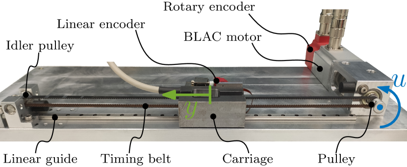
(a) Photograph of experimental setup.

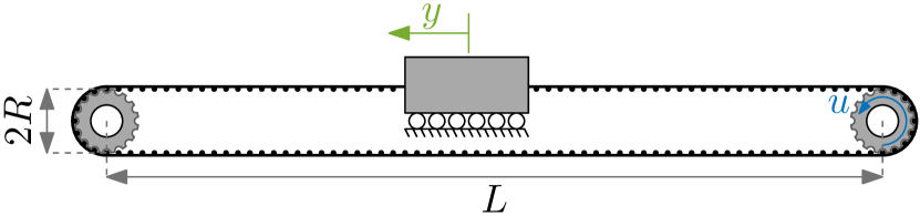
(b) Sketch of experimental setup.

Figure 1: Experimental setup considered, where the position of the belt-driven carriage $y$ is to be controlled using the input to the motor $u$.

The objective of the setup is to accurately position the carriage in the $y$-direction by using the BrushLess AC (BLAC) motor. The BLAC motor is connected to the carriage via a toothed pulley and a timing belt. The belt-driven carriage suffers from position-dependent dynamics due to several effects, including pulley out-of-roundness, pulley-teeth interactions, motor cogging, misalignment of the linear guide, and position-dependent drivetrain stiffness [20, Section 4.2], which is shown in Example 1.

Example 1.

By modeling the timing belt in Figure 1 as an elastic element under pretension with Young’s modulus $E$ and cross-sectional area $A$, the perceived stiffness at the driven pulley is

$$k(\rho)=\frac{EA}{\frac{1}{2}L+\rho R}+\frac{EA}{1\frac{1}{2}L-\rho R},$$ (4)

for scheduling $\rho$ being the angular rotation of the driven pulley, resulting in quasi-LPV behavior. The system is modeled as a mass-spring system with continuous-time inverse dynamics [19]

$$u(t) =\left(mR+\frac{J}{R}\right)\frac{d^{2}y\left(t\right)}{dt^{2}}+\frac{mJ}{R}\frac{d^{2}}{dt^{2}}\left(\frac{1}{k\left(\rho\left(t\right)\right)}\frac{d^{2}y\left(t\right)}{dt^{2}}\right)$$ (5)

$$=\sum_{i\in\{2,3,4\}}\frac{d^{i}y(t)}{dt^{i}}\theta_{i}\left(\rho(t)\right),$$

consisting of derivatives of the desired output $\frac{d^{i}y(t)}{dt^{i}}$ and LPV parameter functions $\theta_{i}\left(\rho(t)\right)$.

LPV descriptions of complex mechatronic systems, including belt-driven carriages such as the system in Figure 1, directly motivate the development of parameter-varying feedforward control.

2.2 Problem Setting

The control structure is seen in Figure 2.

Figure 2: Control structure considered.

The considered class of LPV systems $\mathcal{G}$ is described using the convolution in (3). The system is operating in feedback with LTI controller $\mathcal{C}$, as seen in Figure 2. The tracking error, assuming zero initial state and error, is given by the interconnection of the system $\mathcal{G}$ and controller $\mathcal{C}$ by

$$e(k)=\mathcal{S}\left(\rho\right)\left(r(k)-\nu(k)\right)-\mathcal{J}\left(\rho\right)f(k),$$ (6)

with LPV sensitivity $\mathcal{S}(\rho)$ and process sensitivity $\mathcal{J}(\rho)$. LTI feedforward is not capable of compensating for the LPV dynamics in (6), resulting in residual error. Motivated by the inverse dynamics of LPV systems, for example (5) in Example 1, the goal in this paperis to decrease the tracking error using the parameter-varying feedforward signal

$$f(k)=\psi\left(r\left(k\right)\right)\theta(\rho(k)),$$ (7)

with basis functions $\psi\left(r\left(k\right)\right)\in\mathbb{R}^{1\times n_{\theta}}$ and feedforward parameter functions $\theta(\rho(k))\in\mathbb{R}^{n_{\theta}\times 1}$. The feedforward parameterization (7) is flexible to task variations due to the dependency on $r(k)$ in the basis function $\psi(r(k))$.

2.3 Problem Definition

The problem considered in this paperis as follows. Given a reference signal $r(k)$, corresponding choice of basis functions $\psi\left(r\left(k\right)\right)\in\mathbb{R}^{1\times n_{\theta}}$, a model of the system $\widehat{\mathcal{G}}$, and the measured scheduling sequence $\rho(k)$, determine the $n_{\theta}$ feedforward parameter functions $\theta(\rho(k))\in\mathbb{R}^{n_{\theta}\times 1}$, such that the tracking error (6) is minimized using the feedforward parameterization (7).

3 Learning Feedforward Parameter Functions

In this section, feedforward parameter functions are iteratively learned through kernel-regularized estimation. The non-parametric nature of kernel-regularized estimation enables modeling any dependence on the scheduling sequence, and iterative learning improves estimation quality, both contributing to C1 and C2. Furthermore, the design of kernels and the developed procedure are presented.

3.1 Iterative Learning of Feedforward Parameter Functions

The key idea is to iteratively learn the feedforward parameter functions $\theta(\rho(k))$ in (7) such that the tracking performance is minimized. Hence, the feedforward parameters are iteratively updated over iterations or trials $j$ as

$$\theta_{j+1}(\rho^{*})=\theta_{j}(\rho^{*})+\theta_{j}^{\Delta}(\rho^{*}),$$ (8)

with some arbitrary scheduling value $\rho^{*}$. The tracking error is directly reduced by learning the function $\theta_{j}^{\Delta}(\rho^{*})$ iteratively by minimizing the predicted tracking error in the next trial. To achieve this, the error (6) in the next trial $\hat{e}_{j+1}$ for feedforward signal (7) is predicted by assuming a trial-invariant scheduling sequence $\rho_{j+1}=\rho_{j}$, reference signal $r_{j+1}=r_{j}$ and noise $\nu_{j+1}=\nu_{j}$, i.e.,

$$\hat{e}_{j+1}(k)=\mathcal{S}\left(\rho_{j}\right)\left(r_{j}(k)-\nu_{j}(k)\right)-\widehat{\mathcal{J}}\left(\rho_{j}\right)\psi\left(r_{j}\left(k\right)\right)\theta_{j+1}\left(\rho_{j}\left(k\right)\right),$$ (9)

where $\widehat{\mathcal{J}}\left(\rho_{j}\right)$ is a model of the true system $\mathcal{J}\left(\rho_{j}\right)$, determined using the measured scheduling sequence $\rho_{j}$. Predicting this error based on past data is enabled by substituting $e_{j}$ from (6), resulting in

$$\hat{e}_{j+1}(k) =e_{j}(k)-\widehat{\mathcal{J}}\left(\rho_{j}\right)\psi\left(r_{j}\left(k\right)\right)\left(\theta_{j+1}\left(\rho_{j}\left(k\right)\right)-\theta_{j}\left(\rho_{j}\left(k\right)\right)\right)$$ (10)

$$=e_{j}(k)-\widehat{\mathcal{J}}\left(\rho_{j}\right)\psi\left(r_{j}\left(k\right)\right)\theta_{j}^{\Delta}\left(\rho_{j}\left(k\right)\right).$$

The iterative procedure is effective since it directly minimizes the regularized least-squares tracking error, and uses next to the model of the process sensitivity the measured data, thus reducing the requirements on the modeling quality [21].

3.2 Iterative Kernel-Regularized Learning of Feedforward Parameter Functions

Unlike traditional estimation methods that restrict the estimated function $\theta_{j}^{\Delta}(\rho^{*})$ in (8) to a specific structure, the function $\theta_{j}^{\Delta}(\rho^{*})$ is estimated in a possibly infinite-dimensional function space $\mathscr{H}$ and can be evaluated at any arbitrary $\rho^{*}\in\mathbb{R}$. Specifically, the feedforward parameter functions are estimated by iteratively minimizing the predicted least-squares tracking error (10) with a regularization term $J$ to prevent overfitting and ill-posedness, i.e.,

$$\min_{\theta_{j}^{\Delta}\in\mathscr{H}}\sum_{k=0}^{N-1}\hat{e}_{j+1}^{2}(k)+\gamma J\left(\theta_{j}^{\Delta}\right).$$ (11)

The regularizer $J$ can be chosen to penalize unwanted behavior of the estimated functions $\theta_{j}^{\Delta}$. For example, the energy of the estimated functions $\theta_{j}^{\Delta}$ can be reduced by penalizing with $J(\theta_{j}^{\Delta})=\int{\left(\theta_{j}^{\Delta}(\rho)\right)^{\top}\theta_{j}^{\Delta}(\rho)\;d\rho}$.

Properties of the estimated function are effectively enforced through designing $\mathscr{H}$ as a Hilbert space, and choosing the regularizer as the squared norm in this space,

$$\min_{\theta_{j}^{\Delta}\in\mathscr{H}}\sum_{k=0}^{N-1}\hat{e}_{j+1}^{2}(k)+\gamma\|\theta_{j}^{\Delta}\|_{\mathscr{H}}^{2},$$ (12)

with Reproducing Kernel Hilbert Space (RKHS) norm $\|\theta_{j}^{\Delta}\|_{\mathscr{H}}^{2}=\left\langle\theta_{j}^{\Delta},\theta_{j}^{\Delta}\right\rangle_{\mathscr{H}}$ [17]. The RKHS $\mathscr{H}$ is associated with a kernel function that is capable of reproducing every function in the space, in this case the $n_{\theta}\times n_{\theta}$ kernel function matrix

$$K\left(\rho^{*},\rho\right)=\begin{bmatrix}k_{11}\left(\rho^{*},\rho\right)&k_{12}\left(\rho^{*},\rho\right)&\cdots&k_{1n_{\theta}}\left(\rho^{*},\rho\right)\\ k_{21}\left(\rho^{*},\rho\right)&k_{22}\left(\rho^{*},\rho\right)&\cdots&k_{2n_{\theta}}\left(\rho^{*},\rho\right)\\ \vdots&\vdots&\ddots&\vdots\\ k_{n_{\theta}1}\left(\rho^{*},\rho\right)&k_{n_{\theta}2}\left(\rho^{*},\rho\right)&\cdots&k_{n_{\theta}n_{\theta}}\left(\rho^{*},\rho\right)\end{bmatrix},$$ (13)

where each kernel function $k_{ij}$ describes the correlation between feedforward parameters $i$ and $j$. As a result, the kernel functions enable to enforce desired properties of the estimated function $\theta_{j}^{\Delta}\left(\rho^{*}\right)$, such as smoothness or periodicity.

Remark 2.

Cross-correlation between different feedforward parameters, which is commonly observed for motion systems [19], is directly enabled by setting $k_{ij}\neq 0\;\forall i\neq j$.

Since the kernel-regularized estimates of the feedforward parameter functions are estimated in the possibly infinite dimensional space $\mathscr{H}$, the function estimates are not restricted to a specific class of functions and are thus capable of modeling any feedforward parameter function.

Although the feedforward parameter functions are modeled in a possibly infinite dimensional space $\mathscr{H}$, it admits a finite-dimensional solution through the representer theorem [17, (63)]

$$\theta_{j}^{\Delta}\left(\rho^{*}\right)=\sum_{k=0}^{N-1}K\left(\rho^{*},\rho_{j}(k)\right)\psi^{\top}\left(r_{j}\left(k\right)\right)\widehat{\mathcal{J}}\left(\rho_{j}\right)\hat{c}_{j}(k),$$ (14)

where kernel function matrix $K(\rho^{*},\rho_{j}(k))\in\mathbb{R}^{n_{\theta}\times n_{\theta}}$ is determined with (13). The (modified) representers $\hat{c}_{j}=\begin{bmatrix}\hat{c}_{j}(0)&\hat{c}_{j}(1)&\cdots&\hat{c}_{j}(N-1)\end{bmatrix}^{\top}\in\mathbb{R}^{N}$ are given by [17, (64) and (70b)]

$$\hat{c}_{j}=\left(\widehat{J}_{j}\Psi_{j}K_{j}\Psi_{j}^{\top}{\widehat{J}_{j}}^{\top}+\gamma I_{N}\right)^{-1}e_{j},$$ (15)

with convolution matrix $\widehat{J}_{j}\in\mathbb{R}^{N\times N}$ of LPV system $\widehat{\mathcal{J}}$ evaluated at the measured scheduling sequence $\rho_{j}$ using (3), and the kernel matrix $K_{j}\in\mathbb{R}^{Nn_{\theta}\times Nn_{\theta}}$ is evaluated by

Note that the feedforward parameters for the next trial in (14) are calculated based on the scheduling sequence measured in the current trial. The basis function matrix $\Psi_{j}\in\mathbb{R}^{N\times Nn_{\theta}}$ is constructed such that $f_{j}=\Psi_{j}\theta_{j}$ as

$$\Psi_{j}=\begin{bmatrix}\psi\left(r_{j}\left(0\right)\right)&0&\cdots&0\\ 0&\psi\left(r_{j}\left(1\right)\right)&\cdots&0\\ \vdots&\vdots&\ddots&\vdots\\ 0&\cdots&0&\psi\left(r_{j}\left(N-1\right)\right)\end{bmatrix}.$$ (17)

The feedforward parameters for the next trial (8) are estimated by propagating the feedforward update using the representer theorem (14) over the trials, resulting in

$$\theta_{j+1}\left(\rho^{*}\right)=\sum_{i=0}^{j}\sum_{k=0}^{N-1}K\left(\rho^{*},\rho_{i}(k)\right)\hat{c}_{i}(k).$$ (18)

Kernel-regularized learning of LPV feedforward parameter functions in (18) estimates the functions without restricting the dependence on the scheduling sequence, while allowing for the incorporation of prior knowledge.

Remark 3.

For the special case where the scheduling sequence during iterative learning is constant, i.e., $\rho_{j}(k)=\rho(k)\;\forall j$, the parameter update (18) simplifies to

$$\theta_{j+1}\left(\rho^{*}\right)=\theta_{j}\left(\rho^{*}\right)+\sum_{k=0}^{N-1}K\left(\rho^{*},\rho(k)\right)\hat{c}_{j}(k).$$ (19)

Remark 4.

The convergence of learning feedforward parameter functions (18) is primarily influenced by

1. the quality of model $\widehat{\mathcal{J}}$;

2. the choice of kernel functions in (13); and

3. the regularization coefficient $\gamma$ in (12) and (15).

Generally, the regularization parameter $\gamma$ can be increased to ensure convergence of the framework. Furthermore, ILC with basis functions and its associated convergence properties [22] are recovered by $K\left(\rho^{*},\rho\right)=I$ and $\gamma=0$.

3.3 Design of Kernel Functions

The developed update law requires the design of kernel functions $k_{ij}\left(\rho^{*},\rho\right)$ in matrix $K\left(\rho^{*},\rho\right)$ in (13). Many different kernel functions are possible, and the suitable choice depends on the problem at hand. Three examples of high-level properties that can be enforced on the feedforward parameters through the use of kernel functions are the following.

1. Constant feedforward parameter functions are realized by the constant kernel

   $$k_{ij}^{c}\left(\rho^{*},\rho\right)=\sigma^{2},$$ (20)

   with hyperparameter $\sigma^{2}$ determining the average distance of the function to its mean. The constant kernel recovers LTI ILC with basis functions [21], where Tikhonov regularized estimates are used for the feedforward parameters.

2. Smooth feedforward parameter functions are estimated using the squared-exponential kernel

   $$k_{ij}^{SE}\left(\rho^{*},\rho\right)=\sigma^{2}\exp\left(-\frac{\left(\rho^{*}-\rho\right)^{2}}{2\ell^{2}}\right),$$ (21)

   where $\sigma^{2}$ has the same function as for the kernel (20), and the hyperparameter $\ell$ determines the level of smoothness of the estimated function.

3. Periodic feedforward parameter functions are realized through the periodic kernel

   $$k_{ij}^{per}\left(\rho^{*},\rho\right)=\sigma^{2}\exp\left(-\frac{2\sin^{2}\left(\pi\left|\rho^{*}-\rho\right|/p\right)}{\ell^{2}}\right),$$ (22)

   where $\sigma^{2}$ and $\ell$ have the same role as in the squared-exponential kernel (21), and the hyperparameter $p$ forces the feedforward parameter functions to be periodic with period $p$.

In addition, multiple kernels can be combined such that they have the properties of various kernels, and can be trivially extended for multidimensional inputs [23, 24].

Remark 5.

The LPV feedforward signal should in some cases be dynamically dependent, meaning that it should be dependent on derivatives or time-shifted values of $\rho$ [16, 19]. The kernel functions can be straightforwardly extended by using these values as additional input to the kernel.

3.4 Procedure

The developed procedure that iteratively learns feedforward parameter functions through kernel-regularized estimation is summarized in Procedure 6.

 

Procedure 6 (Iterative kernel-regularized learning of LPV feedforward parameters).

 

Inputs: Model $\widehat{\mathcal{J}}$, reference signal $r_{j}$, choice of basis functions in $\psi$, which (measured) signals are the scheduling sequence $\rho_{j}$, kernel function matrix $K(\rho_{j}^{*},\rho_{j})$ from (13) and corresponding hyperparameters.

1. Initialize $\theta_{0}\left(\rho^{*}\right)$, e.g., $\theta_{0}\left(\rho^{*}\right)=0\;\forall\rho^{*}$.

2. For $j\in\mathbb{Z}_{[0,N_{trial}-1]}$

   1. Compute basis functions $\psi(r_{j}(k))$ in (7) using the reference $r_{j}(k)$, and construct basis function matrix $\Psi_{j}$ using (17).

   2. Compute $f_{j}(k)$ with (7).

   3. Apply $f_{j}(k)$ and $r_{j}(k)$ to the system in Figure 2, and measure error $e_{j}(k)$ and scheduling sequence $\rho_{j}(k)$.

   4. Construct convolution matrix $\widehat{J}_{j}$ using (3) with model $\widehat{\mathcal{J}}$ and measured scheduling sequence $\rho_{j}(k)$.

      • If no LPV model is available, set $\widehat{\mathcal{J}}\left(\rho_{j}\right)$ to an LTI approximate, i.e., $\widehat{\mathcal{J}}(q)$.

   5. Determine kernel matrix $K_{j}$ based on measured scheduling sequence $\rho_{j}$ using (16).

   6. Calculate the representers $\hat{c}_{j}$ for trial $j$ using (15).

   7. Compute the feedforward parameters for the next trial $j+1$ based on the current measured scheduling sequence $\rho_{j}$, meaning $\theta_{j+1}(\rho_{j}(k))$, using (18).

 

4 Experimental Setup Characterization

In this section, the experimental setup is introduced and characterized, leading to an appropriate parameter-varying feedforward parameterization, hence contributing to C3. Specifically, several preliminary experiments are performed to determine which feedforward structure and kernels will be used.

4.1 Experimental Setup

The experimental setup considered is a 1 degree-of-freedom belt-driven carriage, which is mounted on a linear guide, as shown in Section 2.1 and Figure 1. The BLAC motor is equipped with a rotary encoder having a resolution of 8192 counts per revolution, in addition to a linear encoder on the linear guide with a resolution of 100 nm. The timing belt has a tooth pitch of 2 mm, which is made of rubber with an added carbon fiber core for additional stiffness. The pulleys have 15 teeth per revolution, and hence, a circumference of 0.03 m. The distance between the pulleys is $L=0.3$ m. The goal is to track a third-order scanning motion with the carriage using the input to the motor $u$, consisting of a large constant velocity part, which is seen in Figure 3.

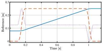
Figure 3: Reference $r$ ( ), scaled reference velocity $\dot{r}$ ( ), and scaled reference acceleration ( ) applied to the experimental setup.

The performance is evaluated during constant velocity, since this type of drivetrain is typically used in scanning applications such as printing systems.

The control scheme in Figure 2 is used, where the LTI feedback controller is a discrete-time lead filter with an additional low-pass filter described by the transfer function

$$\mathcal{C}(q)=\frac{2169q^{-1}-381q^{-2}-1747q^{-3}}{1-2.421q^{-1}+1.961q^{-2}-0.5337q^{-3}}.$$ (23)

The settings during experimentation are shown in Table 1.

Table 1: Experimental settings.

Variable	Abbrevation	Value	Unit
Sampling time	$T_{s}$	$2.5\cdot 10^{-4}$	s
Number of samples	N	4630	-
Reference stroke	-	0.171	m
Maximum velocity	-	0.2	m/s
Maximum acceleration	-	4	m/s2

4.2 Characterization of Position-Dependent Dynamics

The tracking error with zero feedforward $f_{j}=0$ for 5 repetitions of the reference in Figure 3 is shown in Figure 4.

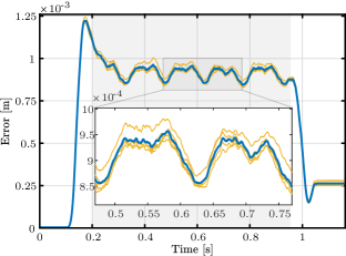
Figure 4: During constant velocity ( ), the experimental tracking error for 5 repetitions of the reference in Figure 3 with zero feedforward $f_{j}=0$ ( ) and their sample mean ( ) show highly repeatable position-dependent effects.

The following is observed from the tracking error in Figure 4.

• The tracking error is highly repeatable, and hence, an iterative approach is suitable.

• The large offset in the tracking error indicates that both Coulomb and viscous friction feedforward might be necessary.

• During acceleration, the error reaches its maximum, motivating the need for acceleration feedforward.

• The tracking error has a period of 0.15 s during a constant velocity of 0.2 m/s, resulting in a spatial period of 0.03 m, which is the circumference of the pulley.

The spatial periodic effect is further analyzed with a power spectrum of the tracking error during constant velocity as a function of the number of pulley revolutions in Figure 5.

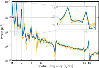
Figure 5: Power spectrum of the tracking error during constant velocity for 5 times tracking the reference in Figure 3 with zero feedforward $f_{j}=0$ ( ) and their sample mean ( ) shows highly repetitive behavior in spatial domain.

The spatial power spectrum shows that during constant velocity, the error is dominated by the zero frequency, the fundamental frequency [1/rev], its second harmonic [2/rev] and marginally by its fourth harmonic [4/rev]. The zero frequency contribution is mainly caused by the lack of Coulomb friction feedforward, which is also seen from the constant offset of the tracking error in Figure 4. The fundamental frequency, and second and fourth harmonic are most likely caused due position-dependent effects introduced by pulley out-of-roundness or motor cogging.

5 Experimental Application

In this section, both LTI feedforward control and the developed LPV feedforward control methods are compared on the experimental setup, further contributing to C3. Both the learning procedure and the tracking results are shown.

5.1 Experimental Learning Settings

The model of the process sensitivity $\widehat{\mathcal{J}}$ is determined by using a simplified LTI model of the system $\mathcal{G}$ in feedback with the controller $\mathcal{C}$ in (23). The simplified LTI model $\widehat{\mathcal{G}}$ is determined by using the measured frequency response function in Figure 6.

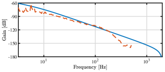
Figure 6: The LTI model $\widehat{\mathcal{G}}(q)$ ( ) is constructed to approximate the measured frequency response function ( ) of the experimental belt-driven carriage.

As a result, the simplified LTI model $\widehat{\mathcal{G}}$ consists of a mass with a damper attached to the fixed world, and is discretized with a zero order hold, resulting in

$$\widehat{\mathcal{G}}(q)=\frac{2.82q^{-1}+2.798q^{-2}}{1-1.978q^{-1}+0.9775q^{-2}}\cdot 10^{-8}.$$ (24)

After interconnecting $\widehat{\mathcal{G}}$ with the controller $\mathcal{C}$ from (23), the LTI model of the process sensitivity is

The reference tracking task is constant during learning $r_{j}=r\;\forall j$ and the same as in Section 4.1, shown in Figure 3. The reference signal is used as scheduling sequence $\rho_{j}=r\;\forall j$, since this is relatively close to the position of the carriage $y$, and it is known in advance of the tracking experiment.

The observations in Section 4.2 motivate using viscous friction, Coulomb friction, and acceleration feedforward in (7), which is widely applied in feedforward control [25], i.e.,

$$f_{j}\left(k\right)=\theta^{a}_{j}\left(\rho\left(k\right)\right)\ddot{r}\left(k\right)+\theta^{v}_{j}\left(\rho\left(k\right)\right)\dot{r}\left(k\right)+\theta^{c}_{j}\left(\rho\left(k\right)\right)\operatorname{sign}\left(\dot{r}\left(k\right)\right),$$ (26)

with discrete-time derivatives $\ddot{r}(k)$ and $\dot{r}(k)$. The corresponding basis functions and feedforward parameters from (7) are

$$\psi\left(r\left(k\right)\right) =\begin{bmatrix}\left(\frac{q-q^{-1}}{2T_{s}}\right)^{2}r(k)&\frac{q-q^{-1}}{2T_{s}}r(k)&\operatorname{sign}\left(\frac{q-q^{-1}}{2T_{s}}r(k)\right)\end{bmatrix},$$ (27)

$$\theta_{j}\left(\rho\left(k\right)\right) =\begin{bmatrix}\theta^{a}_{j}\left(\rho\left(k\right)\right)&\theta^{v}_{j}\left(\rho\left(k\right)\right)&\theta^{c}_{j}\left(\rho\left(k\right)\right)\end{bmatrix}^{\top},$$

where discrete-time derivatives $\ddot{r}(k)$ and $\dot{r}(k)$ from (26) are computed using the central difference. The $3\times 3$ kernel function matrix (13) is defined such that the estimated feedforward parameters $\theta_{j}\left(\rho\left(k\right)\right)$ do not correlate, and the acceleration and Coulomb friction feedforward parameter functions are enforced to be constant using the kernel (20), i.e.,

$$K\left(\rho^{*},\rho\right)=\begin{bmatrix}k^{c}\left(\rho^{*},\rho\right)&0&0\\ 0&k_{22}\left(\rho^{*},\rho\right)&0\\ 0&0&k^{c}\left(\rho^{*},\rho\right)\end{bmatrix}.$$ (28)

The hyperparameters of the constant kernels for the acceleration and coulomb friction feedforward parameter functions are respectively $\sigma^{2}=1$ and $\sigma^{2}=3$. The amount of trials is set to 10 and the regularization coefficient $\gamma$ from (12) to $\gamma=5\cdot 10^{-5}$.

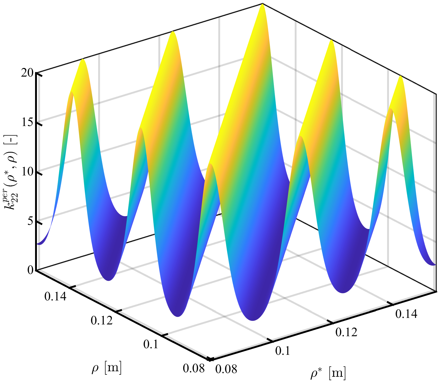
Figure 7: Surface plot of kernel function $k_{22}^{per}(\rho^{*},\rho)$ evaluated at a scheduling sequence $\rho^{*}\!,\rho\in\mathbb{R}_{[0.08,0.16]}$ ( ), which enforces a smooth and periodic function having a period of $p=0.03$ m.

LTI feedforward control and the developed LPV feedforward control are compared by using a constant or varying viscous friction feedforward parameter function. Specifically, the compared methods use the following kernel functions for the viscous friction feedforward parameter.

• LTI feedforward: constant kernel from (20), $k_{22}\left(\rho^{*},\rho\right)=k^{c}\left(\rho^{*},\rho\right)$, with hyperparameter $\sigma^{2}=20$.

• LPV feedforward: periodic kernel from (22), $k_{22}\left(\rho^{*},\rho\right)=k^{per}_{22}\left(\rho^{*},\rho\right),$ with hyperparameters $\sigma^{2}=20$, $\ell=1$ m and $p=3\cdot 10^{-2}$ m.

The spatial periodic effect of the tracking error in Section 4.2 motivates to select $k_{22}$ being periodic in the pulley circumference. A surface plot of the kernel function $k^{per}_{22}$ is shown in Figure 7. LTI feedforward control recovers LTI ILC with basis functions [21], where Tikhonov regularization is used to estimate the feedforward parameters.

5.2 Experimental Results

The learned viscous, Coulomb, and acceleration feedforward parameter functions are shown in Figure 8 and Figure 9.

Figure 8: Feedforward parameter function $\theta_{j}^{v}(\rho(k))$ over the trials estimated by the developed LPV feedforward method ( ) and LTI feedforward method $\theta_{j}^{v}$ ( ).

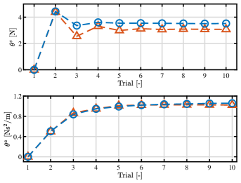
Figure 9: Constant feedforward parameters $\theta^{c}_{j}$ and $\theta^{a}_{j}$ estimated by LTI feedforward control ( ) and LPV feedforward control ( ).

The viscous friction feedforward parameter function clearly shows the periodic behavior enforced by the periodic kernel. The Coulomb friction and acceleration feedforward parameters do not show any significant difference between the LTI and LPV feedforward methods.

The feedforward signal in the final trial from (26) using the feedforward parameters from Figure 8 and Figure 9 for the reference in Figure 3 is shown in Figure 10.

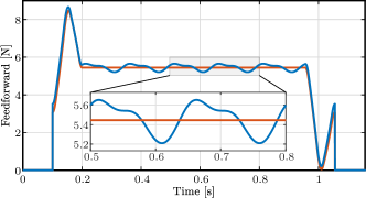
Figure 10: The feedforward signal during the final trial $f_{10}$ shows the periodic effect obtained by the LPV feedforward signal ( ) compared to the LTI feedforward signal ( ).

The reference tracking performance is illustrated through the Root-Mean-Squared (RMS) tracking errors in Figure 11, the tracking error in the final trial in Figure 12, and the power spectrum of the final tracking error in Figure 13. The following observations are made concerning the tracking performance.

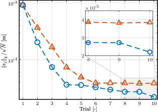
Figure 11: The RMS error during constant velocity converges faster and to a lower value for the developed iterative kernel-regularized estimates of LPV parameters ( ) compared to the LTI feedforward parameters ( ).

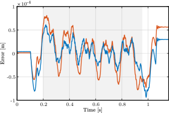
Figure 12: During constant velocity ( ), the tracking error in the final trial $e_{10}$ is reduced by the developed iterative kernel-regularized estimates of LPV feedforward parameters ( ) compared to the LTI feedforward parameters ( ).

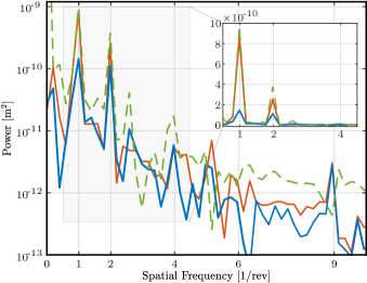
Figure 13: The power of the tracking error for the final trial $e_{10}$ is significantly lower for the developed LPV feedforward control ( ) compared to LTI feedforward control ( ) and zero feedforward $f_{j}=0$ ( ).

• The RMS error during constant velocity decreased from $3.85\cdot 10^{-5}$ m for LTI feedforward parameters to $2.2\cdot 10^{-5}$ m, which is an improvement of 43 %, as shown in Figure 11.

• Figure 12 demonstrates the improved tracking accuracy. In addition, it shows a reduction of the maximum absolute error during constant velocity in the final trial, with $\left\|e_{10}\right\|_{\infty}$ decreasing from $8.1\cdot 10^{-5}$ m to $6.1\cdot 10^{-5}$ m, which is an improvement of 25 %.

• The amplitude of the first and second harmonic are decreased by respectively a factor 6 and 2.3 in terms of their power, as shown in Figure 13.

The observations show that learning feedforward parameter functions using the developed iterative kernel-regularized estimator increases performance significantly for motion systems.

6 Conclusions

The results in this paperenable data-driven learning of parameter-variations in feedforward control, which can significantly improve the tracking performance of LPV systems. The key idea is to iteratively learn LPV feedforward parameter functions using kernel-regularized estimation. Kernel-regularized function estimation is advantageous since it is non-parametric, meaning no specific structure needs to be enforced on the dependency on the scheduling sequence. The iterative learning approach directly optimizes the tracking error, which enhances the estimation quality without the need for accurate system models. The developed framework is experimentally validated on a belt-driven motion system, demonstrating effective compensation of position-dependent drivetrain dynamics. The developed method demonstrates significant potential for industrial applications, particularly in mechatronic systems, by enabling improved tracking performance.

Max van Haren is currently working toward the Ph.D. degree in mechanical engineering with the Control Systems Technology section, Eindhoven University of Technology. He received the M.Sc. degree (cum laude) in mechanical engineering in 2021 from the Eindhoven University of Technology, Eindhoven, The Netherlands. His research interests include control and identification of mechatronic systems, including sampled-data, multirate, and linear parameter-varying systems.

Lennart Blanken is currently a System Designer Mechatronics with Sioux Technologies, Eindhoven, The Netherlands. Additionally, he is an assistant professor with the Department of Mechanical Engineering at the Eindhoven University of Technology. He received the M.Sc. degree (cum laude) and Ph.D. degree in mechanical engineering from the Eindhoven University of Technology, Eindhoven, The Netherlands, in 2015 and 2019, respectively. His research interests include advanced feedforward control, learning control, repetitive control, and their applications to mechatronic systems.

Tom Oomen is full professor with the Department of Mechanical Engineering at the Eindhoven University of Technology. He is also a part-time full professor with the Delft University of Technology. He received the M.Sc. degree (cum laude) and Ph.D. degree from the Eindhoven University of Technology, Eindhoven, The Netherlands. He held visiting positions at KTH, Stockholm, Sweden, and at The University of Newcastle, Australia. He is a recipient of the 7th Grand Nagamori Award, the Corus Young Talent Graduation Award, the IFAC 2019 TC 4.2 Mechatronics Young Research Award, the 2015 IEEE Transactions on Control Systems Technology Outstanding Paper Award, the 2017 IFAC Mechatronics Best Paper Award, the 2019 IEEJ Journal of Industry Applications Best Paper Award, and recipient of a Veni and Vidi personal grant. He is currently a Senior Editor of IEEE Control Systems Letters (L-CSS) and Co-Editor-in-Chief of IFAC Mechatronics, and he has served on the editorial board of IEEE Transactions on Control Systems Technology. He has also been vice-chair for IFAC TC 4.2 and a member of the Eindhoven Young Academy of Engineering. His research interests are in the field of data-driven modeling, learning, and control, with applications in precision mechatronics.

References

- [1] G. M. Clayton, S. Tien, K. K. Leang, Q. Zou, S. Devasia, A Review of Feedforward Control Approaches in Nanopositioning for High-Speed SPM, Journal of Dynamic Systems, Measurement, and Control 131 (6) (2009). https://doi.org/10.1115/1.4000158.
- [2] M. Grotjahn, B. Heimann, Model-based Feedforward Control in Industrial Robotics, The International Journal of Robotics Research 21 (1) (2002) 45–60. https://doi.org/10.1177/027836402320556476.
- [3] S. Devasia, Should model-based inverse inputs be used as feedforward under plant uncertainty?, IEEE Transactions on Automatic Control 47 (11) (2002). https://doi.org/10.1109/TAC.2002.804478.
- [4] M. Groot Wassink, M. van de Wal, C. Scherer, O. Bosgra, LPV control for a wafer stage: beyond the theoretical solution, Control Engineering Practice 13 (2) (2005). https://doi.org/10.1016/j.conengprac.2004.03.008.
- [5] C. Hoffmann, H. Werner, A survey of linear parameter-varying control applications validated by experiments or high-fidelity simulations, IEEE Transactions on Control Systems Technology 23 (2) (2015) 416–433. https://doi.org/10.1109/TCST.2014.2327584.
- [6] B. Bamieh, L. Giarré, Identification of linear parameter varying models, International Journal of Robust and Nonlinear Control 12 (9) (2002) 841–853. https://doi.org/10.1002/rnc.706.
- [7] F. Previdi, M. Lovera, Identification of non-linear parametrically varying models using separable least squares, International Journal of Control 77 (16) (2004) 1382–1392. https://doi.org/10.1080/0020717041233318863.
- [8] R. Tóth, Modeling and Identification of Linear Parameter-Varying Systems, Springer, 2010. https://doi.org/10.1007/978-3-642-13812-6.
- [9] Y. Zhao, B. Huang, H. Su, J. Chu, Prediction error method for identification of LPV models, Journal of Process Control 22 (1) (2012) 180–193. https://doi.org/10.1016/j.jprocont.2011.09.004.
- [10] J. Theis, H. Pfifer, A. Knoblach, F. Saupe, H. Werner, Linear Parameter-Varying Feedforward Control: A Missile Autopilot Design, in: Proceedings of the AIAA Guidance, Navigation, and Control Conference, 2015. https://doi.org/10.2514/6.2015-2001.
- [11] R. de Rozario, T. Oomen, M. Steinbuch, Iterative Learning Control and feedforward for LPV systems: Applied to a position-dependent motion system, in: Proceedings of the American Control Conference, 2017, pp. 3518–3523. https://doi.org/10.23919/ACC.2017.7963491.
- [12] T. Bloemers, I. Proimadis, Y. Kasemsinsup, R. Toth, Parameter-Dependent Feedforward Strategies for Motion Systems, in: Proceedings of the American Control Conference, 2018, pp. 2017–2022. https://doi.org/10.23919/ACC.2018.8431116.
- [13] M. Butcher, A. Karimi, Data-driven tuning of linear parameter-varying precompensators, International Journal of Adaptive Control and Signal Processing 21 (2009). https://doi.org/10.1002/acs.1151.
- [14] R. de Rozario, R. Pelzer, S. Koekebakker, T. Oomen, Accommodating Trial-Varying Tasks in Iterative Learning Control for LPV Systems, Applied to Printer Sheet Positioning, in: Proceedings of the American Control Conference, 2018, pp. 5213–5218. https://doi.org/10.23919/ACC.2018.8430906.
- [15] D. A. Bristow, M. Tharayil, A. G. Alleyne, A survey of iterative learning control, IEEE Control Systems 26 (3) (2006) 96–114. https://doi.org/10.1109/MCS.2006.1636313.
- [16] J. Kon, J. van de Wijdeven, D. Bruijnen, R. Tóth, M. Heertjes, T. Oomen, Direct Learning for Parameter-Varying Feedforward Control: A Neural-Network Approach, in: Proceedings of the 62nd IEEE Conference on Decision and Control, 2023, pp. 3720–3725. https://doi.org/10.1109/CDC49753.2023.10383877.
- [17] G. Pillonetto, F. Dinuzzo, T. Chen, G. De Nicolao, L. Ljung, Kernel methods in system identification, machine learning and function estimation: A survey, Automatica 50 (3) (2014) 657–682. https://doi.org/10.1016/j.automatica.2014.01.001.
- [18] M. van Haren, M. Poot, J. Portegies, T. Oomen, Position-Dependent Snap Feedforward: A Gaussian Process Framework, in: Proceedings of the American Control Conference, 2022, pp. 4778–4783. https://doi.org/10.23919/ACC53348.2022.9867449.
- [19] M. van Haren, L. Blanken, T. Oomen, A kernel-based identification approach to LPV feedforward: With application to motion systems, in: Proceedings of the 22nd World Congress of the IFAC, 2023, pp. 6063–6068. https://doi.org/10.1016/j.ifacol.2023.10.662.
- [20] R. Perneder, I. Osborne, Handbook Timing Belts, Springer, 2012. https://doi.org/10.1007/978-3-642-17755-2.
- [21] S. H. van der Meulen, R. L. Tousain, O. H. Bosgra, Fixed Structure Feedforward Controller Design Exploiting Iterative Trials: Application to a Wafer Stage and a Desktop Printer, Journal of Dynamic Systems, Measurement, and Control 130 (5) (2008) 051006/1–051006/16. https://doi.org/10.1115/1.2957626.
- [22] J. van de Wijdeven, O. Bosgra, Using basis functions in iterative learning control: analysis and design theory, International Journal of Control 83 (4) (2010). https://doi.org/10.1080/00207170903334805.
- [23] C. E. Rasmussen, Gaussian Processes for Machine Learning, MIT Press, 2006.
- [24] D. K. Duvenaud, Automatic Model Construction with Gaussian Processes, Ph.D. thesis, University of Cambridge (2014).
- [25] M. Steinbuch, R. Merry, M. Boerlage, M. Ronde, M. van de Molengraft, Advanced Motion Control Design, in: The Control Handbook, Control System Applications, 2nd Edition, CRC Press, 2010, pp. 27/1–25. https://doi.org/10.1201/b10382-35.