Abstract

This paper proposes AAPG-SPIDER, an Adaptive Accelerated Proximal Gradient (AAPG) method with variance reduction for minimizing composite nonconvex finite-sum functions. It integrates three acceleration techniques: adaptive stepsizes, Nesterov’s extrapolation, and the recursive stochastic path-integrated estimator SPIDER. While targeting stochastic finite-sum problems, AAPG-SPIDER simplifies to AAPG in the full-batch, non-stochastic setting, which is also of independent interest. To our knowledge, AAPG-SPIDER and AAPG are the first learning-rate-free methods to achieve optimal iteration complexity for this class of composite minimization problems. Specifically, AAPG achieves the optimal iteration complexity of $\mathcal{O}(N\epsilon^{-2})$, while AAPG-SPIDER achieves $\mathcal{O}(N+\sqrt{N}\epsilon^{-2})$ for finding $\epsilon$-approximate stationary points, where $N$ is the number of component functions. Under the Kurdyka-Lojasiewicz (KL) assumption, we establish non-ergodic convergence rates for both methods. Preliminary experiments on sparse phase retrieval and linear eigenvalue problems demonstrate the superior performance of AAPG-SPIDER and AAPG compared to existing methods.

1 Introduction

We consider the following composite nonconvex finite-sum minimization problem (where ‘$\triangleq$’ denotes definition):

$$\min_{\mathbf{x}}\,f(\mathbf{x})+h(\mathbf{x}),\,\text{where}\,f(\mathbf{x})\triangleq\frac{1}{N}\sum_{i=1}^{N}f_{i}(\mathbf{x}).$$ (1)

Here, $\mathbf{x}\in\mathbb{R}^{n}$. The function $f(\cdot)$ is assumed to be differentiable, possibly nonconvex. The function $h(\mathbf{x})$ is assumed to be closed, proper, lower semi-continuous, potentially nonconvex, and possibly nonsmooth. Furthermore, we assume the generalized proximal operator of $h(\mathbf{x})$ is easy to compute.

Problem (1) has diverse applications in machine learning. The function $f(\mathbf{x})$ captures empirical loss, including neural network activations, while nonsmooth regularization $h(\mathbf{x})$ prevents overfitting and improves generalization. It incorporates prior information, such as structured sparsity, low-rank properties, discreteness, orthogonality, and non-negativity, enhancing model accuracy. These capabilities extend to various applications, including sparse phase retrieval Cai et al. (2024); Shechtman et al. (2014), eigenvalue problems Wen & Yin (2013), $\ell_{2}$-weight decay in neural networks Zhang et al. (2019), and network quantization Bai et al. (2019).

Table 1: Comparison among existing methods for composite nonconvex funite-sum minimization. The notation $\tilde{\mathcal{O}}(\cdot)$ hides polylogarithmic factors, while $\mathcal{O}(\cdot)$ hides constants.

	Adaptive Stepsize	Nonconvex $h(\mathbf{x})$	Nesterov Extrapol.	Diagonal Precond.	Iteration Complexity	Last-Iterate Convergence Rate
APG Li & Lin (2015)	✘	✔	✔	✘	$\mathcal{O}(N/\epsilon)$	✔
ProxSVRG J. Reddi et al. (2016)	✘	✘	✔	✘	$\mathcal{O}(N+N^{2/3}\epsilon^{-2})$	unknown
SVRG-APG Li et al. (2017)	✘	✔	✔	✘	unknowna	✔
SPIDER Fang et al. (2018)	✘	✘	✘	✔	$\mathcal{O}(N+\sqrt{N}\epsilon^{-2})$	unknown
SpiderBoost Wang et al. (2019)	✘	✔	✔	✘	$\mathcal{O}(N+\sqrt{N}\epsilon^{-2})$	unknown
ProxSARAH Pham et al. (2020)	✘	✘	✘	✘	$\mathcal{O}(N+\sqrt{N}\epsilon^{-2})$	unknown
AdaGrad-Norm Ward et al. (2020)	✔	✘	✘	✘	$\mathcal{O}(N\epsilon^{-2})$	unknown
AGD Kavis et al. (2022a)	✔	✘	✔	✘	$\mathcal{O}(N\epsilon^{-2})$	unknown
ADA-SPIDER Kavis et al. (2022b)	✔	✘	✘	✘	$\tilde{\mathcal{O}}(N+\sqrt{N}\epsilon^{-2})$	unknown
AAPG [ours]	✔	✔	✔	✔	$\mathcal{O}(N\epsilon^{-2})$	✔ [Theorem 4.8]
AAPG-SPIDER [ours]	✔	✔	✔	✔	$\mathcal{O}(N+\sqrt{N}\epsilon^{-2})$	✔ [Theorem 4.13]

Note $a$: This work only demonstrates that any cluster point is a critical point but fail to establish the iteration complexity.

Stochastic Gradient Descent and Variance Reduction Methods. In many applications, the finite-sum minimization problem often involves both $n$ and $N$ being large. First-order methods have become the standard choice for solving Problem (1) due to their efficiency. Vanilla gradient descent (GD) requires $\mathcal{O}(N\epsilon^{-2})$ gradient evaluations, while Stochastic Gradient Descent (SGD) demands $\mathcal{O}(N\epsilon^{-4})$ gradient computations in total Ghadimi & Lan (2013); Ghadimi et al. (2016); Ghadimi & Lan (2016). To harness the advantages of both GD and SGD, the variance reduction (VR) framework Johnson & Zhang (2013); Schmidt et al. (2013) was introduced. This framework combines the faster convergence of GD with the lower per-iteration complexity of SGD by decomposing the finite-sum structure into manageable components. VR methods generate low-variance gradient estimates by balancing periodic full-gradient computations with stochastic mini-batch gradients. Notable approaches, including SAGA Defazio et al. (2014); J. Reddi et al. (2016), SVRG Johnson & Zhang (2013); Li & Li (2018), SARAH Nguyen et al. (2017), SPIDER Fang et al. (2018), SNVRG Zhou et al. (2020), and PAGE Li et al. (2021), have been developed. While earlier work achieved an iteration complexity of $\mathcal{O}(N+N^{2/3}\epsilon^{-2})$ with a suboptimal dependence on $N$, recent methods Fang et al. (2018); Pham et al. (2020) have improved this to the optimal iteration complexity of $\mathcal{O}(N+N^{1/2}\epsilon^{-2})$.

Adaptive Stepsizes. The choice of stepsize is critical in optimization, affecting both convergence speed and stability. Traditional fixed or manually tuned stepsizes often underperform on complex non-convex problems, resulting in suboptimal outcomes. Adaptive stepsize methods McMahan & Streeter (2010); Duchi et al. (2011), such as Adam Kingma & Ba (2015); Chen et al. (2022), and AdaGrad Duchi et al. (2011), mitigate these issues by dynamically adjusting the stepsize based on gradient information. Recent advancements, including Polyak stepsize Wang et al. (2023); Jiang & Stich (2024), Barzilai-Borwein stepsize Zhou et al. (2024), scaled stepsize Oikonomidis et al. (2024), and D-adaptation Defazio & Mishchenko (2023), have primarily focused on convex optimization. This work extends adaptive stepsize techniques Duchi et al. (2011) to address composite non-convex finite-sum minimization problems.

Nesterov Extrapolation. Nesterov’s extrapolation method is a foundational technique in optimization, celebrated for its ability to accelerate gradient-based algorithms Nesterov (2003); Beck & Teboulle (2009). By incorporating a momentum-based step, it achieves an optimal convergence rate for smooth convex functions, outperforming traditional gradient descent. This technique has been extended to solve nonconvex problems Ghadimi & Lan (2016); Li & Lin (2015); Yang (2023); Qian & Pan (2023), particularly in training deep neural networks Sutskever et al. (2013), where it enhances convergence efficiency while keeping the computational cost nearly unchanged.

Diagonal Preconditioner. Diagonal preconditioners are employed by popular adaptive gradient methods such as ADAM. Unlike identity or full matrix preconditioners, diagonal preconditioners approximate the preconditioning matrix using only its diagonal elements, greatly reducing computational cost while preserving the key benefits of adaptivity. By adjusting learning rates for each parameter based on gradient history, diagonal preconditioners assign higher learning rates to parameters with less frequent updates. This adaptive mechanism is especially beneficial for large-scale problems involving sparse or structured models Duchi et al. (2011); Yun et al. (2021).

Theory on Nonconvex Optimization. (i) Iteration complexity. We aim to establish the iteration complexity (or oracle complexity) of nonconvex optimization algorithms, i.e., the number of iteration required to find an $\epsilon$-approximate first-order stationary point $\dot{\mathbf{x}}$ satisfying ${\rm{dist}}(\mathbf{0},\partial(f+g)(\dot{\mathbf{x}}))\leq\epsilon$. However, the iteration complexity of adaptive stepsize methods for solving Problem (1) remains unknown. Existing related work, such as AdaGrad-Norm Ward et al. (2020), AGD Kavis et al. (2022a), and ADA-SPIDER Kavis et al. (2022b), addresses the special case $h(\cdot)=0$, while methods such as APG Li & Lin (2015), ProxSVRG J. Reddi et al. (2016), Spider Fang et al. (2018), SpiderBoost Wang et al. (2019), and ProxSARAH Pham et al. (2020) rely on non-adaptive stepsizes. Our proposed methods, AAPG-SPIDER and AAPG, with and without variance reduction, respectively, address the general case where $h(\mathbf{x})$ is nonconvex, using an adaptive stepsize strategy. Additionally, our methods exploit Nesterov’s extrapolation and leverage diagonal preconditioner techniques. (ii) Last-iterate convergence rate. The work of Attouch & Bolte (2009) establishes a unified framework to prove the convergence rates of descent methods under the Kurdyka-Lojasiewicz (KL) assumption for problem (1). Recent works Qian & Pan (2023); Yang (2023) extend this to nonmonotone descent methods. Inspired by these works, we establish the optimal iteration complexity and derive non-ergodic convergence rates for our methods.

Contributions. We provide a detailed comparison of existing methods for composite nonconvex finite-sum minimization in Table 1. Our main contributions are summarized as follows. (i) We proposes AAPG-SPIDER, an Adaptive Accelerated Proximal Gradient method with variance reduction for composite nonconvex finite-sum optimization. It integrates adaptive stepsizes, Nesterov’s extrapolation, and the SPIDER estimator for fast convergence. In the full-batch setting, it simplifies to AAPG, which is of independently significant (see Section 2). (ii) We show that AAPG-SPIDER and AAPG are the first learning-rate-free methods achieving optimal iteration complexity for this class of composite minimization problems (see Section 3). (iii) Under the Kurdyka-Lojasiewicz (KL) assumption, we establish non-ergodic convergence rates for both methods (see Section 4). (iv) We validate our approaches through experiments on sparse phase retrieval and the linear eigenvalue problem, showcasing its effectiveness (see Section 5).

Notations. Vector operations are performed element-wise. Specifically, for any $\mathbf{x},\mathbf{y}\in\mathbb{R}^{n}$, the operations $(\mathbf{x}+\mathbf{y})$, $(\mathbf{x}-\mathbf{y})$, $(\mathbf{x}\odot\mathbf{y})$, and $(\mathbf{x}\div\mathbf{y})$ represent element-wise addition, subtraction, multiplication, and division, respectively. We use $\|\mathbf{x}\|_{\mathbf{v}}$ to denote the generalized vector norm, defined as $\|\mathbf{x}\|_{\mathbf{v}}=\sqrt{\sum_{i=1}\mathbf{x}_{i}^{2}\mathbf{v}_{i}}$. The notations, technical preliminaries, and relevant lemmas are provided in Appendix Section A.

2 The Proposed Algorithms

This section provides the proposed AAPG-SPIDER algorithm, an Adaptive Accelerated Proximal Gradient method with variance reduction for solving Problem (1). Notably, AAPG-SPIDER reduces to AAPG in the full-batch, non-stochastic setting.

First of all, our algorithms are based on the following assumptions imposed on Problem (1).

Assumption 2.1.

The generalized proximal operator: $\operatorname{\operatorname{Prox}}_{h}(\mathbf{a};\mathbf{v})\triangleq\arg\min_{\mathbf{x}}h(\mathbf{x})+\tfrac{1}{2}\|\mathbf{x}-\mathbf{a}\|_{\mathbf{v}}^{2}$ can be exactly and efficiently for all $\mathbf{a},\mathbf{v}\in\mathbb{R}^{n}$.

Remark 2.2.

(i) Assumption 2.1 is commonly employed in nonconvex proximal gradient methods. (ii) When $\mathbf{v}=\mathbf{1}$, the diagonal preconditioner reduces to the identity preconditioner. Assumption 2.1 holds for certain functions of $h(\mathbf{x})$. Common examples include capped-$\ell_{1}$ penalty Zhang (2010b), log-sum penalty Candes et al. (2008), minimax concave penalty Zhang (2010a), Geman penalty Geman & Yang (1995), $\ell_{p}$ regularization with $p\in\{0,\tfrac{1}{2},\tfrac{2}{3},1\}$, and indicator functions for cardinality constraints, orthogonality constraints in matrices, and rank constraints in matrices. (iii) When $\mathbf{v}$ is a general vector, the variable metric operator can still be evaluated for certain coordinate-wise separable functions of $h(\mathbf{x})$. Examples includes the $\ell_{p}$ norm with $p\in\{0,\tfrac{1}{2},\tfrac{2}{3},1\}$ (with or without bound constraints) Yun et al. (2021) and W-shaped regularizer Bai et al. (2019).

Given any solution $\mathbf{y}^{t}$, we use the SPIDER estimator, introduced by Fang et al. (2018), to approximate its stochastic gradient:

$$\mathbf{g}^{t}=\left\{\begin{array}[]{ll}\nabla f(\mathbf{y}^{t}),&\hbox{$\textrm{mod}(t,q)=0$;}\\ \mathbf{g}^{t-1}+\tilde{\Delta}^{t},&\hbox{else.}\end{array}\right.$$ (4)

where $\tilde{\Delta}^{t}\triangleq\nabla f(\mathbf{y}^{t};\mathcal{I}^{t})-\nabla f(\mathbf{y}^{t-1};\mathcal{I}^{t})$. Here, $\nabla f(\mathbf{y};\mathcal{I}^{t})$ represents the average gradient computed over the examples in $\mathcal{I}^{t}$ at the point $\mathbf{y}$. The mini-batch $\mathcal{I}^{t}$ is selected uniformly at random (with replacement) from the set $\{1,2,...,N\}$ with $|\mathcal{I}^{t}|=b$ for all $t$.

The algorithm, AAPG, and its variant, AAPG-SPIDER, form an adaptive proximal gradient optimization framework designed for composite optimization problems. This framework initializes parameters and iteratively updates the solution by computing gradients (either directly or via a variance-reduced SPIDER estimator) and applying a proximal operator. Both algorithms dynamically update the stepsize factor $\mathbf{v}^{t}$ based on a combination of past differences in iterates. Additionally, the algorithm incorporates momentum-like updates through the extrapolation parameter $\sigma^{t}$ to improve convergence speed. These algorithms are designed for efficient and adaptive optimization in both deterministic and stochastic settings. We present AAPG and AAPG-SPIDER in Algorithm 1.

Algorithm 1 AAPG and AAPG-SPIDER

1: Initialize $\mathbf{x}^{0}$. Let $\mathbf{x}^{-1}=\mathbf{x}^{0}$.

2: Let $\underline{\rm{v}}>0,\alpha>0$, $\beta\geq 0$, and $\theta\in[0,1)$.

3: Set $\mathbf{v}^{0}=\underline{\rm{v}}\mathbf{1}$, $\mathbf{y}^{0}=\mathbf{x}^{0}$, $\sigma^{-1}=\theta$.

4: for $t=0$ to $T$ do

5:  Option AAPG: Compute $\mathbf{g}^{t}=\nabla f(\mathbf{y}^{t})$.

6:  Option AAPG-SPIDER: Compute $\mathbf{g}^{t}$ using (4).

7:  Let $\mathbf{x}^{t+1}\in\operatorname{\operatorname{Prox}}_{h}(\mathbf{y}^{t}-\mathbf{g}^{t}\div{\mathbf{v}^{t}};\mathbf{v}^{t})$, $\mathbf{d}^{t}\triangleq\mathbf{x}^{t+1}-\mathbf{x}^{t}$.

8:  Let $\mathbf{s}^{t}\triangleq\alpha\|\mathbf{r}^{t}\|_{2}^{2}+\beta\mathbf{r}^{t}\odot\mathbf{r}^{t}$, where $\mathbf{r}^{t}\triangleq\mathbf{v}^{t}\odot\mathbf{d}^{t}$.

9:  Set $\mathbf{v}^{t+1}=\sqrt{\mathbf{v}^{t}\odot\mathbf{v}^{t}+\mathbf{s}^{t}}$.

10:  Let $\sigma^{t}\triangleq\theta(1-\sigma^{t-1})\cdot\min(\mathbf{v}^{t}\div\mathbf{v}^{t+1})$.

11:  Set $\mathbf{y}^{t+1}=\mathbf{x}^{t+1}+\sigma^{t}\mathbf{d}^{t}$.

12: end for

Remark 2.3.

(i) The recursive update rule for $\mathbf{v}^{t}$, given by $\mathbf{v}^{t+1}=\sqrt{\mathbf{v}^{t}\odot\mathbf{v}^{t}+\mathbf{s}^{t}}$, can be equivalently expressed as $\mathbf{v}^{t+1}=\textstyle\sqrt{\mathbf{v}^{0}\odot\mathbf{v}^{0}+\textstyle\sum_{i=0}^{t}\mathbf{s}^{t}}$. (ii) The first-order optimality condition of $\mathbf{x}^{t+1}$ is $\mathbf{0}\in\partial h(\mathbf{x}^{t+1})+\mathbf{v}^{t}\odot(\mathbf{x}^{t+1}-\mathbf{a}^{t})$, where $\mathbf{a}^{t}=\mathbf{y}^{t}-\mathbf{g}^{t}\div\mathbf{v}^{t}$. (iii) We examine the special case where $h(\cdot)=0$ and $\beta=\theta=0$ for AAPG, which leads to $\mathbf{y}^{t}=\mathbf{x}^{t}$ and $\mathbf{v}^{t}\odot(\mathbf{x}^{t+1}-\mathbf{x}^{t})=-\mathbf{g}^{t}$. Consequently, the update rule for $\mathbf{v}^{t}$ reduces to $\mathbf{v}^{t+1}=\sqrt{(\mathbf{v}^{0})^{2}+\alpha\textstyle\sum_{i=0}^{t}\|\mathbf{g}^{i}\|_{2}^{2}}$, which is essentially a lazy update of AdaGrad-Norm Ward et al. (2020) that $\mathbf{v}^{t+1}=\sqrt{\textstyle(\mathbf{v}^{0})^{2}+\alpha\textstyle\sum_{i=0}^{t+1}\|\mathbf{g}^{i}\|_{2}^{2}}$. (iv) We address the non-smoothness of $h(\mathbf{x})$ using its (generalized) proximal operator, the basis of proximal gradient methods, which update the parameter via the gradient of $f(\mathbf{x})$ followed by a (generalized) proximal mapping of $h(\mathbf{x})$. (v) The proximal mapping step incorporates an extrapolated point, combining the current and previous points, following the Nesterov’s extrapolation method.

3 Iteration Complexity

This section details the oracle complexity of AAPG and AAPG-SPIDER. AAPG-SPIDER generates a random output $\mathbf{x}^{t}$ with $t=\{0,1,\ldots\}$, based on the observed realizations of the random variable $\varsigma^{t-1}\triangleq\{\mathcal{I}^{0},\mathcal{I}^{1},\ldots,\mathcal{I}^{t-1}\}$. The expectation of a random variable is denoted by $\mathbb{E}_{\varsigma^{t-1}}[\cdot]=\mathbb{E}[\cdot]$, where the subscript is omitted for simplicity.

In the sequel of the paper, we make the following assumptions.

Assumption 3.1.

Each $f_{j}(\cdot)$ is $L$-smooth, meaning that $\|\nabla f_{j}(\mathbf{x})-\nabla f_{j}(\tilde{\mathbf{x}})\|\leq L\|\mathbf{x}-\tilde{\mathbf{x}}\|$ for all $j\in[N]$. This property extends to $f(\mathbf{x})$, which is also $L$-smooth.

Assumption 3.2.

Let $\{\mathbf{x}^{t}\}_{t=0}^{T}$ be generated by Algorithm 1, with $\|\mathbf{x}^{t}\|\leq\overline{\rm{x}}$ for all $t$.

Remark 3.3.

Assumption 3.1 is a standard requirement in the convergence analysis of nonconvex algorithms. Assumption 3.2 is satisfied if the function $(f+h)(\mathbf{x})$ is coercive or if $h(\mathbf{x})$ includes the indicator of a compact set.

We now provide an initial theoretical analysis applicable to both algorithms, followed by a detailed, separate analysis for each.

3.1 Initial Theoretical Analysis

We first establish key properties of $\mathbf{v}^{t}$ and $\sigma^{t}$ utilized in Algorithm 1.

Lemma 3.4.

(Proof in Section B.1, Properties of $\mathbf{v}^{t}$) We define $\mathcal{R}_{t}\triangleq\sum_{i=0}^{t}\|\mathbf{r}^{i}\|_{2}^{2}\in\mathbb{R}$. For all $t\geq 0$, we have:

1. $\sqrt{\underline{\rm{v}}^{2}+\alpha\mathcal{R}_{t}}\leq\mathbf{v}^{t+1}\leq\sqrt{\underline{\rm{v}}^{2}+(\alpha+\beta)\mathcal{R}_{t}}\triangleq\mathcal{V}_{t+1}$.

2. $\tfrac{\max(\mathbf{v}^{t})}{\min(\mathbf{v}^{t})}\leq\dot{\kappa}\triangleq 1+\sqrt{\beta/\alpha}$.

3. $\tfrac{\min(\mathbf{v}^{t+1})}{\min(\mathbf{v}^{t})}\leq\ddot{\kappa}\triangleq 1+2\dot{\kappa}\overline{\rm{x}}\sqrt{\alpha+\beta}$.

Lemma 3.5.

(Proof in Section B.2, Properties of $\sigma^{t}$) For all $t\geq 0$, we have the following results.

1. $\theta(1-\theta)/(\dot{\kappa}\ddot{\kappa})\leq\sigma^{t}\leq\theta$.

2. $(\sigma^{t-1}-1)\mathbf{v}^{t}+\sigma^{t}\mathbf{v}^{t+1}\leq-(1-\theta)^{2}\mathbf{v}^{t}$.

We let $\bar{\mathbf{x}}\in\arg\min_{\mathbf{x}}F(\mathbf{x})$, where $F(\mathbf{x})\triangleq f(\mathbf{x})+h(\mathbf{x})$. We now derive an approximate sufficient descent condition for the sequence

$$\mathcal{Z}_{t}\triangleq\mathbb{E}[F(\mathbf{x}^{t})-F(\bar{\mathbf{x}})+\tfrac{1}{2}\|\mathbf{x}^{t}-\mathbf{x}^{t-1}\|_{\sigma^{t-1}(\mathbf{v}^{t}+L)}^{2}].$$

Lemma 3.6.

(Proof in Section B.3, Properties of $\mathcal{Z}_{t}$) We define $c_{1}\triangleq\tfrac{1}{2}(\tfrac{1-\theta}{\dot{\kappa}})^{2}$, $c_{2}\triangleq\tfrac{3L}{2}$. We have:

$$\mathcal{Z}_{t+1}-\mathcal{Z}_{t}\leq\mathbb{E}[\langle\mathbf{d}^{t},\nabla f(\mathbf{y}^{t})-\mathbf{g}^{t}\rangle+c_{2}\mathbb{S}_{2}^{t}-c_{1}\mathbb{S}_{1}^{t}],$$ (5)

where $\mathbb{S}_{1}^{t}\triangleq\tfrac{\|\mathbf{r}^{t}\|_{2}^{2}}{\min(\mathbf{v}^{t})}$, $\mathbb{S}_{2}^{t}\triangleq\tfrac{\|\mathbf{r}^{t}\|_{2}^{2}}{\min(\mathbf{v}^{t})^{2}}$.

We now derive the upper bounds for the summation of the terms $\mathbb{S}_{1}^{t}$ and $\mathbb{S}_{2}^{t}$ as referenced in Lemma 3.6.

Lemma 3.7.

(Proof in Section B.4) We define $\mathcal{V}_{t}$ as in Lemma 3.4. We have the following results.

1. $\sum_{t=0}^{T}\mathbb{S}_{1}^{t}\leq s_{1}\mathcal{V}_{T+1}$, where $s_{1}\triangleq 2\ddot{\kappa}$.

2. $\sum_{t=0}^{T}\mathbb{S}_{2}^{t}\leq s_{2}\sqrt{\mathcal{V}_{T+1}}$, where $s_{2}\triangleq\tfrac{4\ddot{\kappa}^{2}}{\alpha}\underline{\rm{v}}^{-1/2}$.

3.2 Analysis for AAPG

This subsection provides the convergence analysis of AAPG.

The following lemma is crucial to our analysis.

Lemma 3.8.

(Proof in Section B.5, Boundedness of $\mathcal{Z}_{t}$ and $\mathcal{V}_{t}$) We have the following results for all $t\geq 0$:

1. It holds $\mathcal{Z}_{t}\leq\overline{\mathcal{Z}}$ for some positive constant $\overline{\mathcal{Z}}$.

2. It holds $\mathcal{V}_{t}\leq\overline{\rm{v}}$ for some positive constant $\overline{\rm{v}}$.

Finally, we present the following results on iteration complexity.

Theorem 3.9.

(Proof in Section B.6, Iteration Complexity). Let the sequence $\{\mathbf{x}^{t}\}_{t=0}^{T}$ be generated by AAPG.

1. We have $\sum_{t=0}^{T}\|\mathbf{x}^{t+1}-\mathbf{x}^{t}\|_{2}^{2}\leq\overline{\rm{X}}\triangleq\tfrac{1}{\alpha}((\overline{\rm{v}}/\underline{\rm{v}})^{2}-1)$.

2. We have $\tfrac{1}{T+1}\sum_{t=0}^{T}\|\nabla f(\mathbf{x}^{t+1})+\partial h(\mathbf{x}^{t+1})\|=\mathcal{O}(1/\sqrt{T})$. In other words, there exists $\bar{t}\in[T]$ such that $\|\nabla f(\mathbf{x}^{\bar{t}})+\partial h(\mathbf{x}^{\bar{t}})\|\leq\epsilon$, provided $T\geq\mathcal{O}(\tfrac{1}{\epsilon^{2}})$.

Remark 3.10.

Theorem 3.9 establishes the first optimal iteration complexity result for learning-rate-free methods in deterministically minimizing composite functions.

3.3 Analysis for AAPG-SPIDER

This subsection provides the convergence analysis of AAPG-SPIDER.

We fix $q\geq 1$. For all $t\geq 0$, we denote $r_{t}\triangleq\lfloor\tfrac{t}{q}\rfloor+1$ , leading to $(r_{t}-1)q\leq t\leq r_{t}q-1$.

We introduce an auxiliary lemma from Fang et al. (2018).

Lemma 3.11.

(Lemma 1 in Fang et al. (2018)) The SPIDER estimator produces a stochastic gradient $\mathbf{g}^{t}$ that, for all $t$ with $(r_{t}-1)q\leq t\leq r_{t}q-1$, we have: $\mathbb{E}[\|\mathbf{g}^{t}-\nabla f(\mathbf{y}^{t})\|_{2}^{2}]-\|\mathbf{g}^{t-1}-\nabla f(\mathbf{y}^{t-1})\|_{2}^{2}\leq\tfrac{L^{2}}{b}Y_{t-1}$, where $Y_{i}\triangleq\mathbb{E}[\|\mathbf{y}^{i+1}-\mathbf{y}^{i}\|_{2}^{2}]$.

Based on Lemma 3.6, we have the following results for AAPG-SPIDER.

Lemma 3.12.

(Proof in Appendix B.7) For any positive constant $\phi$, we define $c_{1}\triangleq\tfrac{1}{2}(\tfrac{1-\theta}{\dot{\kappa}})^{2}$, $c^{\prime}_{2}\triangleq\tfrac{(3+\phi)L}{2}$, $c_{3}\triangleq\tfrac{L}{2\phi}\tfrac{q}{b}$. We define $Y_{i}\triangleq\mathbb{E}[\|\mathbf{y}^{i+1}-\mathbf{y}^{i}\|_{2}^{2}]$. For all $t$ with $(r_{t}-1)q\leq t\leq r_{t}q-1$, we have:

1. $\mathbb{E}[\|\mathbf{g}^{t}-\nabla f(\mathbf{y}^{t})\|_{2}^{2}]\leq\tfrac{L^{2}}{b}\sum_{i=(r_{t}-1)q}^{t-1}Y_{i}$.

2. $\mathcal{Z}_{t+1}-\mathcal{Z}_{t}+\mathbb{E}[c_{1}\mathbb{S}_{1}^{t}-c^{\prime}_{2}\mathbb{S}_{2}^{t}]\leq\textstyle\tfrac{c_{3}}{q}\sum_{i=(r_{t}-1)q}^{t-1}Y_{i}$.

Based on Lemma 3.7, we obtain the following results.

Lemma 3.13.

(Proof in Appendix B.8) We define $V_{t}\triangleq\min(\mathbf{v}^{t})$, and $Y_{i}\triangleq\mathbb{E}[\|\mathbf{y}^{i+1}-\mathbf{y}^{i}\|_{2}^{2}]$. We have:

1. $\sum_{t=0}^{T}V_{t}Y_{t}\leq u_{1}\mathbb{E}[\mathcal{V}_{T+1}]$, where $u_{1}\triangleq(8+2\ddot{\kappa})s_{1}$.

2. $\sum_{t=0}^{T}Y_{t}\leq u_{2}\mathbb{E}[\sqrt{\mathcal{V}_{T+1}}]$, where $u_{2}\triangleq 10s_{2}$.

The following lemma simplifies the analysis by reducing double summations involving $V_{i}$ and $Y_{i}$ to single summations, thereby facilitating the bounding of cumulative terms.

Lemma 3.14.

(Proof in Appendix B.9) We define $Y_{i}\triangleq\mathbb{E}[\|\mathbf{y}^{i+1}-\mathbf{y}^{i}\|_{2}^{2}]$, $V_{i}\triangleq\min(\mathbf{v}^{i})$, and $q^{\prime}\triangleq q\ddot{\kappa}^{q-1}$. For all $t$ with $(r_{t}-1)q\leq t\leq r_{t}q-1$, we have:

1. $\sum_{j={(r_{t}-1)q}}^{t}[V_{j}\sum_{i=(r_{j}-1)q}^{j-1}Y_{i}]\leq q^{\prime}\sum_{i=(r_{t}-1)q}^{t-1}V_{i}Y_{i}$.

2. $\sum_{j=(r_{t}-1)q}^{t}[\sum_{i=(r_{j}-1)q}^{j-1}Y_{i}]\leq(q-1)\sum_{i=(r_{t}-1)q}^{t-1}Y_{i}$.

3. $\sum_{t=0}^{T}[\sum_{i=(r_{t}-1)q}^{t-1}Y_{i}]\leq(q-1)\sum_{t=1}^{T}Y_{t}$.

We derive the following critical lemma, which is analogous to Lemma 3.8.

Lemma 3.15.

(Proof in Appendix B.10, Boundedness of $\mathcal{Z}_{t}$ and $\mathcal{V}^{t}$) We have the following results for all $t\geq 0$:

1. It holds $\mathbb{E}[\mathcal{Z}_{t}]\leq\overline{\mathcal{Z}}$ for some positive constant $\overline{\mathcal{Z}}$.

2. It holds $\mathbb{E}[\mathcal{V}^{t}]\leq\overline{\rm{v}}$ for some positive constant $\overline{\rm{v}}$.

Finally, we provide the following results on iteration complexity.

Theorem 3.16.

(Proof in Section B.11, Iteration Complexity). Let the sequence $\{\mathbf{x}^{t}\}_{t=0}^{T}$ be generated by Algorithm 1.

1. We have $\mathbb{E}[\sum_{t=0}^{T}\|\mathbf{x}^{t+1}-\mathbf{x}^{t}\|_{2}^{2}]\leq\overline{\rm{X}}\triangleq\tfrac{1}{\alpha}((\overline{\rm{v}}/\underline{\rm{v}})^{2}-1)$.

2. We have $\mathbb{E}[\tfrac{1}{T+1}\sum_{t=0}^{T}\|\nabla f(\mathbf{x}^{t+1})+\partial h(\mathbf{x}^{t+1})\|]\leq\mathcal{O}(1/\sqrt{T})$. In other words, there exists $\bar{t}\in[T]$ such that $\mathbb{E}[\|\nabla f(\mathbf{x}^{\bar{t}})+\partial h(\mathbf{x}^{\bar{t}})\|]\leq\epsilon$, provided $T\geq\tfrac{1}{\epsilon^{2}}$.

3. Assume $b=q=\sqrt{N}$. The total stochastic first-order oracle complexity required to find an $\epsilon$-approximate critical point, satisfying $\mathbb{E}[\|\nabla f(\mathbf{x}^{\bar{t}})+\partial h(\mathbf{x}^{\bar{t}})\|]\leq\epsilon$, is given by $\mathcal{O}(N+\sqrt{N}\epsilon^{-2})$.

Remark 3.17.

(i) The work of Kavis et al. (2022b) introduces the first learning-rate-free variance-reduced method, ADA-SPIDER, for solving Problem (1) with $h(\cdot)=0$. However, its oracle complexity, $\tilde{\mathcal{O}}(N+\sqrt{N}\epsilon^{-2})$, is sub-optimal. In contrast, the proposed AAPG-SPIDER successfully eliminates the logarithmic factor in ADA-SPIDER, achieving optimal iteration complexity. (ii) Theorem 3.16 establishes the first optimal iteration complexity result for learning-rate-free methods in minimizing composite finite-sum functions.

4 Convergence Rate

This section presents the convergence rates of AAPG and AAPG-SPIDER, leveraging the non-convex analysis tool known as the Kurdyka-Lojasiewicz (KL) assumption Attouch et al. (2010); Bolte et al. (2014); Li & Lin (2015); Li et al. (2023); Qian & Pan (2023).

We make the following additional assumptions.

Assumption 4.1.

The function $\mathcal{Z}(\mathbf{x},\mathbf{x}^{\prime},\sigma,\mathbf{v})\triangleq F(\mathbf{x})-F(\bar{\mathbf{x}})+\tfrac{1}{2}\|\mathbf{x}-\mathbf{x}^{\prime}\|_{\sigma(\mathbf{v}+L)}^{2}$ is a KL function with respect to $\mathbb{W}\triangleq\{\mathbf{x},\mathbf{x}^{\prime},\sigma,\mathbf{v}\}$.

We present the following useful lemma, due to Attouch et al. (2010); Bolte et al. (2014).

Lemma 4.2.

(Kurdyka-Łojasiewicz Inequality). For a KL function $\mathcal{Z}(\mathbb{W})$ with $\mathbb{W}\in\operatorname{dom}(\mathcal{Z})$, there exists $\tilde{\eta}\in(0,+\infty)$, $\tilde{\sigma}\in[0,1)$, a neighborhood $\Upsilon$ of $\mathbb{W}^{\infty}$, and a continuous concave desingularization function $\varphi(s)\triangleq\tilde{c}s^{1-\tilde{\sigma}}$ with $\tilde{c}>0$ and $s\in[0,\tilde{\eta})$ such that, for all $\mathbb{W}\in\Upsilon$ satisfying $\mathcal{Z}(\mathbb{W})-\mathcal{Z}(\mathbb{W}^{\infty})\in(0,\tilde{\eta})$, it holds that:

$$\varphi^{\prime}(\mathcal{Z}(\mathbb{W})-\mathcal{Z}(\mathbb{W}^{\infty}))\cdot{\rm{dist}}(\mathbf{0},\partial\mathcal{Z}(\mathbb{W}))\geq 1.$$

Remark 4.3.

All semi-algebraic and subanalytic functions satisfy the KL assumption. Examples of semi-algebraic functions include real polynomial functions, $\|\mathbf{x}\|_{p}$ for $p\geq 0$, the rank function, the indicator function of Stiefel manifolds, the positive-semidefinite cone, and matrices with constant rank.

We provide the following lemma on subgradient bounds at each iteration.

Lemma 4.4.

(Proof in Appendix C.1, Subgradient Lower Bound for the Iterates Gap) We define $\mathbb{W}^{t}=\{\mathbf{x}^{t},\mathbf{x}^{t-1},\sigma^{t-1},\mathbf{v}^{t}\}$. We have $\|\partial\mathcal{Z}(\mathbb{W}^{t+1})\|\leq\vartheta(\|\mathbf{x}^{t+1}-\mathbf{x}^{t}\|+\|\mathbf{x}^{t}-\mathbf{x}^{t-1}\|)$.

4.1 Analysis for AAPG

This subsection presents the convergence rate for AAPG. We define $X_{t}\triangleq\|\mathbf{x}^{t}-\mathbf{x}^{t-1}\|$. We define $S_{t}\triangleq\sum_{j=t}^{\infty}X_{j+1}$. The following assumption is used in the analysis.

Assumption 4.5.

There exists a sufficiently large index $t_{\star}$ such that $\xi\triangleq c_{1}\min(\mathbf{v}^{t_{\star}})-c_{2}>0$.

Remark 4.6.

Assumption 4.5 holds if $\min(\mathbf{v}^{t_{\star}})>\tfrac{c_{2}}{c_{1}}=\tfrac{3\dot{\kappa}^{2}L}{(1-\theta)^{2}}$, which requires $\min(\mathbf{v}^{t_{\star}})$ to be over a multiple of $L$ and is relatively mild.

We establish a finite-length property of AAPG, which is significantly stronger than the result in Theorem 3.9.

Theorem 4.7.

(Proof in Appendix C.2, Finite-Length Property). We define $\varphi_{t}\triangleq\varphi(\mathcal{Z}(\mathbb{W}^{t})-\mathcal{Z}(\mathbb{W}^{\infty}))$. We define $\vartheta$ in Lemma 4.4. We define $\xi$ in Assumption 4.5. For all $t\geq t_{\star}$, we have:

1. It holds that $X_{t+1}^{2}\leq\tfrac{\vartheta}{\xi}(X_{t}+X_{t-1})(\varphi_{t}-\varphi_{t+1})$.

2. It holds that $\forall i\geq t$, $S_{i}\leq\varpi(X_{i}+X_{i-1})+\varpi\varphi_{i}$, where $\varpi>0$ is some constant. The sequence $\{X_{j}\}_{j=t}^{\infty}$ has the finite length property that $S_{t}$ is always upper-bounded by a certain constant.

3. For all $t\geq 0$, we have: $\|\mathbf{x}^{t}-\mathbf{x}^{\infty}\|\leq S_{t}$.

Finally, we establish the last-iterate convergence rate for AAPG.

Theorem 4.8.

(Proof in Appendix C.3, Convergence Rate). There exists $t^{\prime}$ such that for all $t\geq t^{\prime}$, we have:

1. If $\tilde{\sigma}=0$, then the sequence $\mathbf{x}^{t}$ converges in a finite number of steps.

2. If $\tilde{\sigma}\in(0,\tfrac{1}{2}]$, then there exist $\dot{\varsigma}\in(0,1)$ such that $\|\mathbf{x}^{t}-\mathbf{x}^{\infty}\|=\mathcal{O}(\dot{\varsigma}^{t})$.

3. If $\tilde{\sigma}\in(\tfrac{1}{2},1)$, then it follows that $\|\mathbf{x}^{t}-\mathbf{x}^{\infty}\|\leq\mathcal{O}(t^{-\dot{\varsigma}})$, where $\dot{\varsigma}\triangleq\tfrac{1-\tilde{\sigma}}{2\tilde{\sigma}-1}>0$.

Remark 4.9.

Under Assumption 4.2, with the desingularizing function $\varphi(t)=\tilde{c}t^{1-\tilde{\sigma}}$ for some $\tilde{c}>0$ and $\tilde{\sigma}\in[0,1)$, Theorem 4.8 establishes that AAPG converges in a finite number of iterations when $\tilde{\sigma}=0$, achieves linear convergence for $\tilde{\sigma}\in(0,\tfrac{1}{2}]$, and exhibits sublinear convergence for $\tilde{\sigma}\in(\tfrac{1}{2},1)$ in terms of the gap $\|\mathbf{x}^{t}-\mathbf{x}^{\infty}\|$. These findings are consistent with the results reported in Attouch et al. (2010).

4.2 Analysis for AAPG-SPIDER

This subsection presents the convergence rate for AAPG-SPIDER. We define $X_{i}\triangleq\sqrt{\sum^{iq-1}_{j=iq-q}\|\mathbf{d}^{j}\|_{2}^{2}}$, and $S_{t}\triangleq\sum_{j=t}^{\infty}X_{j}$. The following assumption is introduced.

Assumption 4.10.

There exists a sufficiently large index $t_{\star}$ such that $\xi\triangleq c_{1}\min(\mathbf{v}^{t_{\star}})-c^{\prime}_{2}-2\xi^{\prime}>0$, where $\xi^{\prime}\triangleq 5c_{3}$, $\{c_{2}^{\prime},c_{3}\}$ are defined in Lemma 3.12.

Remark 4.11.

Assume $q=b$ and $\phi=1$, we have $c_{3}=\tfrac{L}{2}$ and $c_{2}^{\prime}=2L$. Assumption 4.10 is satisfied if $\min(\mathbf{v}^{t_{\star}})>\tfrac{10c_{3}+c^{\prime}_{2}}{c_{1}}=\tfrac{14\dot{\kappa}^{2}L}{(1-\theta)^{2}}$, requiring $\min(\mathbf{v}^{t_{\star}})$ to exceed a multiple of $L$, which is relatively mild.

We now establish the finite-length property of AAPG-SPIDER.

Theorem 4.12.

(Proof in Appendix C.4, Finite-Length Property). Assume $q\geq 2$. We define $\vartheta$ in Lemma 4.4. We define $\{\xi,\xi^{\prime}\}$ in Assumption 4.10. We let $\varphi_{t}\triangleq\varphi(\mathcal{Z}(\mathbb{W}^{t})-\mathcal{Z}(\mathbb{W}^{\infty}))$. We have:

1. It holds that $X^{2}_{r_{t}}+\tfrac{\xi^{\prime}}{\xi}(X^{2}_{r_{t}}-X^{2}_{r_{t}-1})\leq\tfrac{2q\vartheta}{\xi}(\varphi^{(r_{t}-1)q}-\varphi^{r_{t}q})(X_{r_{t}}-X_{r_{t}-1})$.

2. It holds that $\forall i\geq 1$, $S_{i}\leq\varpi X_{i-1}+\varpi\varphi_{(i-1)q}$, where $\varpi>0$ is some constant. The sequence $\{X_{t}\}_{t=0}^{\infty}$ has the finite length property that $S_{t}$ is always upper-bounded by a certain constant.

3. For all $t\geq 1$, we have: $\textstyle\|\mathbf{x}^{tq}-\mathbf{x}^{\infty}\|\leq\sqrt{q}S_{t+1}$.

Finally, we establish the last-iterate convergence rate for AAPG-SPIDER.

Theorem 4.13.

(Proof in Appendix C.5, Convergence Rate). Assume $q\geq 2$. There exists $t^{\prime}$ such that for all $t\geq t^{\prime}$, we have:

1. If $\tilde{\sigma}=0$, then the sequence $\mathbf{x}^{t}$ converges in a finite number of steps in expectation.

2. If $\tilde{\sigma}\in(0,\tfrac{1}{2}]$, then there exist $\dot{\tau}\in[0,1)$ such that $\mathbb{E}[\|\mathbf{x}^{tq}-\mathbf{x}^{\infty}\|]\leq\mathcal{O}(\dot{\tau}^{t})$.

3. If $\tilde{\sigma}\in(\tfrac{1}{2},1)$, then it follows that $\mathbb{E}[\|\mathbf{x}^{tq}-\mathbf{x}^{\infty}\|]\leq\mathcal{O}(t^{-\dot{\tau}})$, where $\dot{\tau}\triangleq\tfrac{1-\tilde{\sigma}}{2\tilde{\sigma}-1}>0$.

Remark 4.14.

(i) Theorem 4.13 mirrors Theorem 4.8, and AAPG-SPIDER shares similar convergence rate as AAPG. (ii) Unlike AAPG, which is assessed at every iteration $\mathbf{x}^{t}$, the convergence rate of AAPG-SPIDER is evaluated only at specific checkpoints $\mathbf{x}^{tq}$, where $q\geq 2$. (iii) No existing work examines the last-iterate convergence rate of VR methods, except for the SVRG-APG method Li et al. (2017), a double-looped approach. However, its reliance on objective-based line search limits its practicality for stochastic optimization, and its (Q-linear) convergence rate is established only for the specific case where the KL exponent is $1/2$. Importantly, their results do not extend to our AAPG-SPIDER method.

5 Experiments

This section presents numerical comparisons of AAPG-SPIDER for solving the sparse phase retrieval problem and AAPG for addressing the linear eigenvalue problem, benchmarked against state-of-the-art methods on both real-world and synthetic datasets.

All methods are implemented in MATLAB and tested on an Intel 2.6 GHz CPU with 64 GB of RAM. The experiments are conducted on a set of 8 datasets, including both randomly generated data and publicly available real-world datasets. Details on the data generation process can be found in Appendix Section D. We compare the objective values of all methods after running for $T$ seconds, where $T$ is chosen to be sufficiently large to ensure the convergence of the compared methods. The code is provided in the supplemental material.

5.1 AAPG-SPIDER on Sparse Phase Retrieval

Sparse phase retrieval seeks to recover a signal $\mathbf{x}\in\mathbb{R}^{n}$ from magnitude-only measurements $\mathbf{y}_{i}=|\langle\mathbf{x},\mathbf{A}_{i}\rangle|^{2}$, where $\mathbf{A}_{i}\in\mathbb{R}^{n}$ are known measurement vectors and $\mathbf{y}_{i}$ are their squared magnitudes. To address this problem, we incorporate sparsity regularization, resulting in the following optimization model: $\min_{\mathbf{x}}\,h(\mathbf{x})+\frac{1}{N}\sum_{i=1}^{N}(\langle\mathbf{x},\mathbf{A}_{i}\rangle^{2}-\mathbf{y}_{i})^{2}$. The regularization term $h(\mathbf{x})$ enforces sparsity using the capped-$\ell_{1}$ penalty Zhang (2010b) while incorporating bound constraints. It is defined as $h(\mathbf{x})\triangleq\iota_{\Omega}(\mathbf{x})+\dot{\lambda}\|\max(|\mathbf{x}|,\tau)\|_{1}$, where $\Omega\triangleq\{\mathbf{x}\,|\,\|\mathbf{x}\|_{\infty}\leq\dot{r}\}$ with $\dot{r},\dot{\lambda}>0$.

$\blacktriangleright$ Compared Methods. We compare AAPG-SPIDER with three state-of-the-art general-purpose algorithms designed to solve Problem (1). (i) ProxSARAH Pham et al. (2020), (ii) SpiderBoost and its Nesterov’s extrapolation version SpiderBoost-M Wang et al. (2019), and (iii) SGP-SPIDER a sub-gradient projection method Yang et al. (2020) using the SPIDER estimator.

$\blacktriangleright$ Experimental Settings. We set the parameters for the optimization problem as $(\dot{r},\dot{\delta})=(10,0.1)$ and vary $\dot{\lambda}\in\{0.01,0.001\}$. For ProxSARAH, and SpiderBoost, and SpiderBoost-M, SGP-SPIDER, we report results using a fixed step size of $0.1$. For AAPG-SPIDER, we use the parameter configuration $(\underline{\rm{v}},\alpha,\beta)=(0.05,0.01,1)$, and evaluate its performance for different values of $\theta\in\{0,0.1,0.5,0.9\}$.

$\blacktriangleright$ Experimental Results. The experimental results depicted in Figures 4 and 4 offer the following insights. (i) The proposed method, AAPG-SPIDER, converges more quickly than the other methods. (i) AAPG-SPIDER-($\theta$) consistently outperforms AAPG-SPIDER-($0$), particularly when $\theta$ is close to, but less than, $1$.

5.2 AAPG on Linear Eigenvalue Problem

Given a symmetric matrix $\mathbf{C}\in\mathbb{R}^{\dot{d}\times\dot{d}}$ and an arbitrary orthogonal matrix $\mathbf{V}\in\mathbb{R}^{\dot{d}\times\dot{r}}$, the trace of $\mathbf{V}^{\mathsf{T}}\mathbf{C}\mathbf{V}$ is minimized when the columns of $\mathbf{V}$ forms an orthogonal basis for the eigenspace corresponding to the $\dot{d}$ smallest eigenvalues of $\mathbf{C}$. Let $\bm{\lambda}_{1}\leq\ldots\leq\bm{\lambda}_{n}<0$ be the eigenvalues of $\mathbf{C}$. The problem of finding the $r$ smallest eigenvalues can be formulated as: $\min_{\mathbf{V}\in\mathbb{R}^{\dot{d}\times\dot{r}}}\operatorname{tr}(\mathbf{V}^{\mathsf{T}}\mathbf{C}\mathbf{V})+\operatorname{tr}(\mathbf{C}),\,s.t.\,\mathbf{X}^{\mathsf{T}}\mathbf{X}=\mathbf{I}_{\dot{d}}$.

$\blacktriangleright$ Compared Methods. We compare AAPG with three state-of-the-art methods: APG Li & Lin (2015), FOForth Gao et al. (2018), and OptM Wen & Yin (2013). For FOForth, different retraction strategies are employed to handle the orthogonality constraint, resulting in several variants: FOForth-GR, FOForth-P, and FOForth-QR. Similarly, for OptM, both QR and Cayley retraction strategies are utilized, giving rise to two variants: OptM-QR and OptM-Cayley. It is worth noting that both FOForth and OptM incorporate the Barzilai-Borwein non-monotonic line search in their implementations.

$\blacktriangleright$ Experimental Settings. For both OptM and FOForth, we utilize the implementations provided by their respective authors, using the default solver settings. For AAPG, we configure the parameters as $(\underline{\rm{v}},\alpha,\beta)=(0.001,0.001,0)$. The performance of all methods is evaluated with varying $\dot{r}\in\{20,50\}$.

$\blacktriangleright$ Experimental Results. Figures 4 and 4 show the comparisons of objective values for different methods with varying $\dot{r}\in\{20,50\}$. Several conclusions can be drawn. (i) The methods OptM, FOForth, and APG generally deliver comparable performance, with none consistently achieving better results than the others. (i) The proposed AAPG method typically demonstrates superior performance compared to all other methods. (iii) AAPG-($\theta$) consistently achieves better results than AAPG-($0$), particularly when $\theta$ is close to, but less than, 1. This underscores the importance of Nesterov’s extrapolation strategy in addressing composite minimization problems.

6 Conclusions

This paper introduces AAPG-SPIDER, an Adaptive Accelerated Proximal Gradient method that leverages variance reduction to address the composite nonconvex finite-sum minimization problem. AAPG-SPIDER combines adaptive stepsizes, Nesterov’s extrapolation, and the SPIDER estimator to achieve enhanced performance. In the full-batch, non-stochastic setting, it reduces to AAPG. We show that AAPG attains an optimal iteration complexity of $\mathcal{O}(N/\epsilon^{2})$, while AAPG-SPIDER achieves $\mathcal{O}(N+\sqrt{N}/\epsilon^{2})$ for finding $\epsilon$-approximate stationary points, making them the first learning-rate-free methods to achieve optimal iteration complexity for this class of problems. Under the Kurdyka-Lojasiewicz (KL) assumption, we establish non-ergodic convergence rates for both methods. Preliminary experiments on sparse phase retrieval and linear eigenvalue problems demonstrate the superior performance of AAPG-SPIDER and AAPG over existing methods.

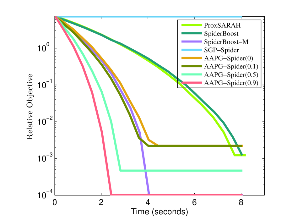
(a) tdt2-9000-1000

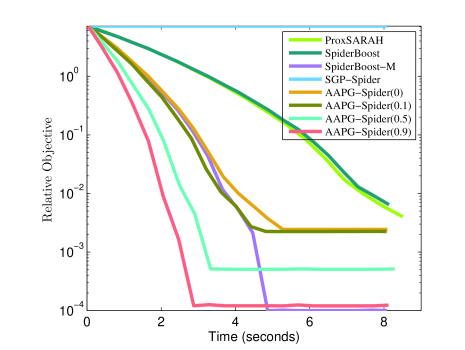
(b) 20news-10000-1000

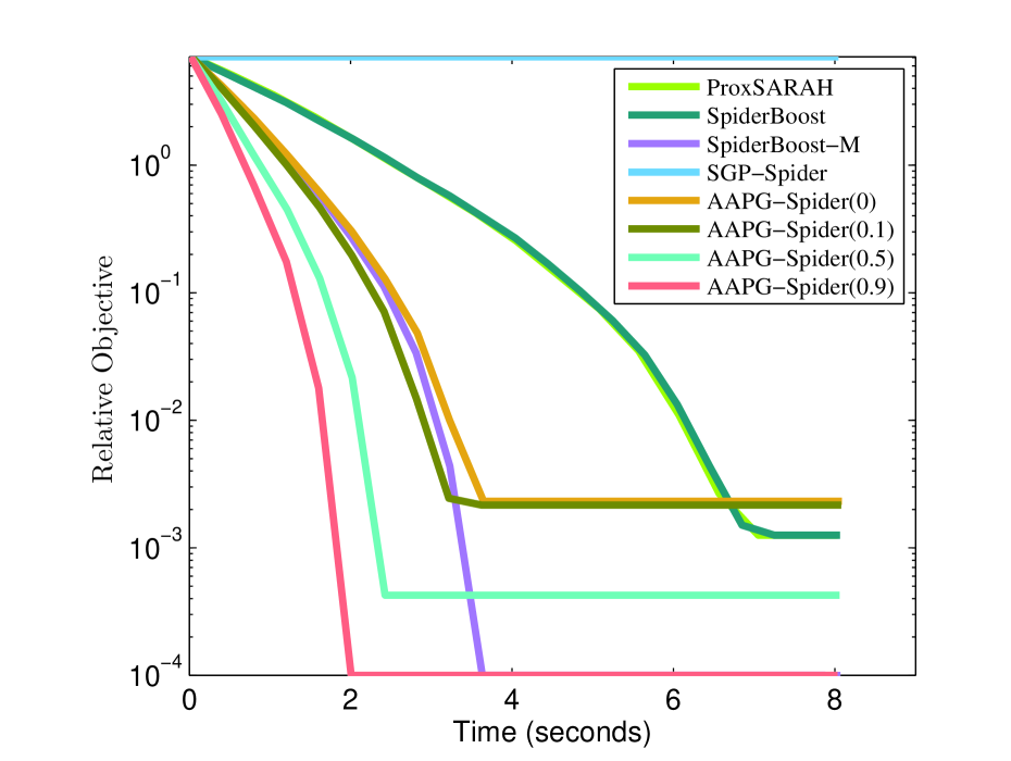
(c) sector-6412-1000

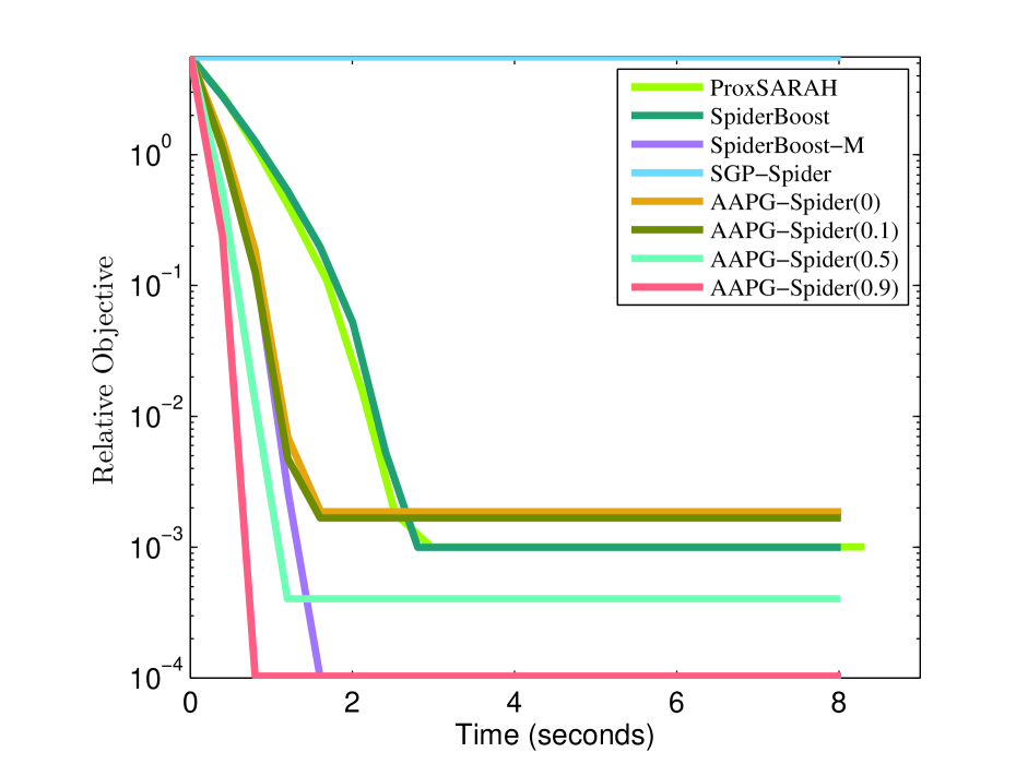
(d) mnist-2000-784

Figure 1: The convergence curve of the compared methods for sparse phase retrieval with $\dot{\lambda}=0.01$.

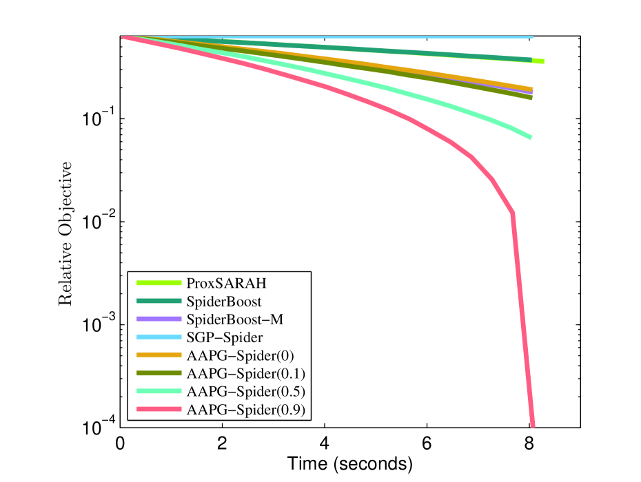
(e) tdt2-9000-1000

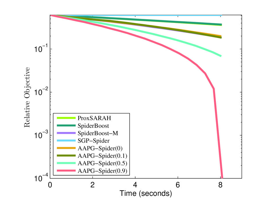
(f) 20news-10000-1000

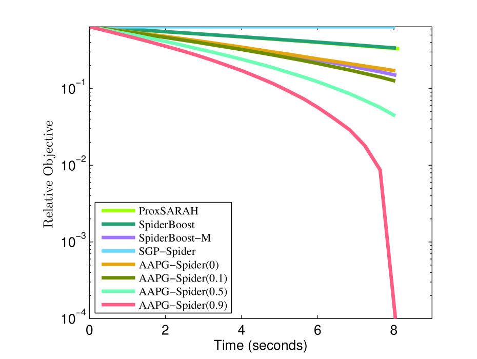
(g) sector-6412-1000

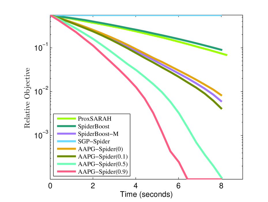
(h) mnist-2000-784

Figure 2: The convergence curve of the compared methods for sparse phase retrieval with $\dot{\lambda}=0.001$.

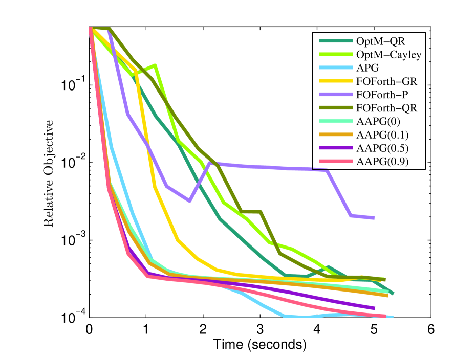
(a) tdt2-3000-3000

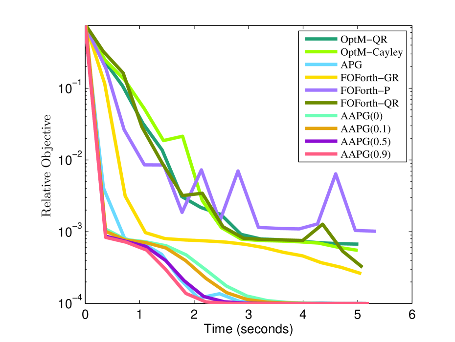
(b) 20news-5000-1000

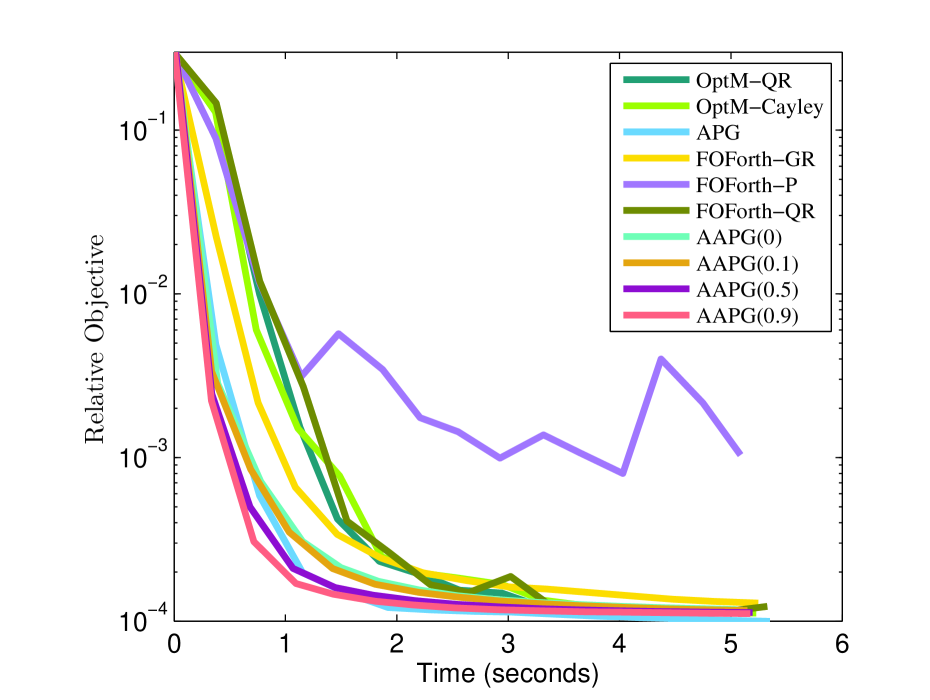
(c) sector-6000-1000

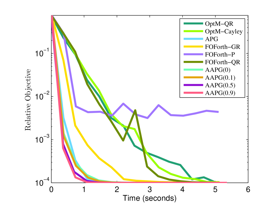
(d) mnist-5000-784

Figure 3: The convergence curve of the compared methods for linear eigenvalue problems with $\dot{r}=20$.

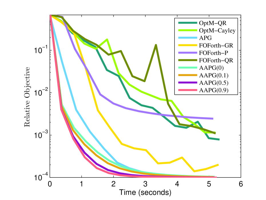
(a) tdt2-3000-3000

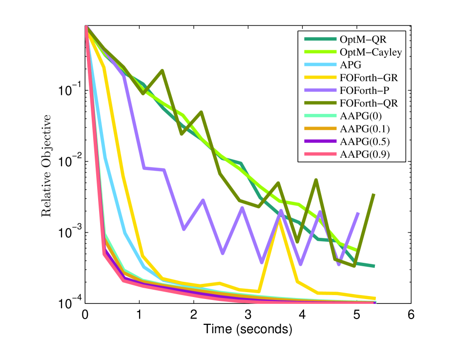
(b) 20news-5000-1000

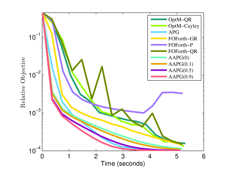
(c) sector-6000-1000

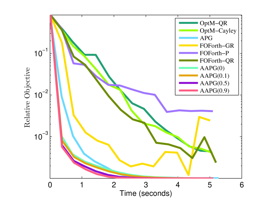
(d) mnist-5000-784

Figure 4: The convergence curve of the compared methods for linear eigenvalue problems with $\dot{r}=50$.

Appendix

The organization of the appendix is as follows:

Appendix A provides notations, technical preliminaries, and relevant lemmas.

Appendix B offers proofs related to Section 3.

Appendix C contains proofs related to Section 4.

Appendix D includes additional experiments details and results.

Appendix A Notations, Technical Preliminaries, and Relevant Lemmas

A.1 Notations

In this paper, bold lowercase letters represent vectors, and uppercase letters denote real-valued matrices. The following notations are used throughout this paper.

• $[n]$: The set $\{1,2,...,n\}$.

• $\|\mathbf{x}\|$: Euclidean norm, defined as $\|\mathbf{x}\|=\|\mathbf{x}\|_{2}=\sqrt{\langle\mathbf{x},\mathbf{x}\rangle}$.

• $\langle\mathbf{a},\mathbf{b}\rangle$ : Euclidean inner product, given by $\langle\mathbf{a},\mathbf{b}\rangle=\sum_{i}{\mathbf{a}_{i}\mathbf{b}_{i}}$.

• $\langle\mathbf{a},\mathbf{b}\rangle_{\mathbf{v}}$ : Generalized inner product, defined as $\langle\mathbf{a},\mathbf{b}\rangle_{\mathbf{v}}=\sum_{i}\mathbf{a}_{i}\mathbf{b}_{i}\mathbf{v}_{i}$.

• $\|\mathbf{x}\|_{\mathbf{v}}$: Generalized vector norm, defined as $\|\mathbf{x}\|_{\mathbf{v}}=\sqrt{\sum_{i=1}\mathbf{x}_{i}^{2}\mathbf{v}_{i}}$.

• $\mathbf{a}\leq\alpha$: For $\mathbf{a}\in\mathbb{R}^{n}$ and $\alpha\in\mathbb{R}$, this means $\mathbf{a}_{i}\leq\alpha$ for all $i\in n$.

• $\iota_{\Omega}(\mathbf{\mathbf{x}})$ : Indicator function of a set $\Omega$ with $\iota_{\Omega}(\mathbf{\mathbf{x}})=0$ if $\mathbf{\mathbf{x}}\in\Omega$ and otherwise $+\infty$.

• $\mathbb{E}[v]$: Expected value of the random variable $v$.

• $\{A_{i}\}_{i=0}^{\infty}$, $\{B_{i}\}_{i=0}^{\infty}$: sequences indexed by the integers $i=0,1,2,3,\ldots$.

• ${\rm{dist}}(\Omega,\Omega^{\prime})$ : distance between two sets with ${\rm{dist}}(\Omega,\Omega^{\prime})\triangleq\inf_{\mathbf{w}\in\Omega,\mathbf{w}^{\prime}\in\Omega^{\prime}}\|\mathbf{w}-\mathbf{w}^{\prime}\|$.

• $\|\partial h(\mathbf{x})\|$: distance from the origin to $\partial h(\mathbf{x})$ with $\|\partial h(\mathbf{x})\|=\inf_{\mathbf{y}\in\partial h(\mathbf{x})}\|\mathbf{y}\|={\rm{dist}}(\mathbf{0},\partial h(\mathbf{x}))$.

• $\mathbf{A}^{\mathsf{T}}$ : the transpose of the matrix $\mathbf{A}$.

• $b$: The mini-batch size parameter of AAPG-SPIDER.

• $q$: The frequency parameter of AAPG-SPIDER (that determines when the full gradient is computed).

A.2 Technical Preliminaries

We introduce key concepts from nonsmooth analysis, focusing on the Fréchet subdifferential and the limiting (Fréchet) subdifferential Mordukhovich (2006); Rockafellar & Wets. (2009); Bertsekas (2015). Let $F:\mathbb{R}^{n}\rightarrow(-\infty,+\infty]$ be an extended real-valued, not necessarily convex function. The domain of $F(\cdot)$ is defined as $\text{dom}(F)\triangleq\{\mathbf{x}\in\mathbb{R}^{n}:|F(\mathbf{x})|<+\infty\}$. The Fréchet subdifferential of $F$ at $\mathbf{x}\in\text{dom}(F)$, denoted as $\hat{\partial}F(\mathbf{x})$, is given by

$$\hat{\partial}{F}(\mathbf{x})\triangleq\{\mathbf{v}\in\mathbb{R}^{n}:\lim_{\mathbf{z}\rightarrow\mathbf{x}}\inf_{\mathbf{z}\neq\mathbf{x}}\frac{{F}(\mathbf{z})-{F}(\mathbf{x})-\langle\mathbf{v},\mathbf{z}-\mathbf{x}\rangle}{\|\mathbf{z}-\mathbf{x}\|}\geq 0\}.$$

The limiting subdifferential of $F(\cdot)$ at $\mathbf{x}\in\text{dom}({F})$, denoted $\partial{F}(\mathbf{x})$, is defined as:

$$\partial{F}(\mathbf{x})\triangleq\{\mathbf{v}\in\mathbb{R}^{n}:\exists\mathbf{x}^{k}\rightarrow\mathbf{x},{F}(\mathbf{x}^{k})\rightarrow{F}(\mathbf{x}),\mathbf{v}^{k}\in\hat{\partial}{F}(\mathbf{x}^{k})\rightarrow\mathbf{v},\forall k\}.$$

It is important to note that $\hat{\partial}{F}(\mathbf{x})\subseteq\partial{F}(\mathbf{x})$. If $F(\cdot)$ is differentiable at $\mathbf{x}$, then $\hat{\partial}{F}(\mathbf{x})=\partial{F}(\mathbf{x})=\{\nabla F(\mathbf{x})\}$, where $\nabla F(\mathbf{x})$ represents the gradient of $F(\cdot)$ at $\mathbf{x}$. For convex function $F(\cdot)$, both $\hat{\partial}{F}(\mathbf{x})$ and $\partial{F}(\mathbf{x})$ reduce to the classical subdifferential for convex functions: $\hat{\partial}{F}(\mathbf{x})=\partial{F}(\mathbf{x})=\{\mathbf{v}\in\mathbb{R}^{n}:F(\mathbf{z})-F(\mathbf{x})-\langle\mathbf{v},\mathbf{z}-\mathbf{x}\rangle\geq 0,\forall\mathbf{z}\in\mathbb{R}^{n}\}$.

A.3 Relevant Lemmas

We provide a set of useful lemmas, each independent of context and specific methodologies.

Lemma A.1.

(Pythagoras Relation) For any vectors $\mathbf{a},\mathbf{v},\mathbf{x},\mathbf{x}^{+}\in\mathbb{R}^{n}$, we have:

$$\tfrac{1}{2}\|\mathbf{x}-\mathbf{a}\|_{\mathbf{v}}^{2}-\tfrac{1}{2}\|\mathbf{x}^{+}-\mathbf{a}\|_{\mathbf{v}}^{2}=\tfrac{1}{2}\|\mathbf{x}-\mathbf{x}^{+}\|_{\mathbf{v}}^{2}+\langle\mathbf{a}-\mathbf{x}^{+},\mathbf{x}^{+}-\mathbf{x}\rangle_{\mathbf{v}}.$$

Lemma A.2.

For all $a,b\geq 0$ and $c,d>0$, we have: $\frac{a+b}{c+d}\leq\max(\tfrac{a}{c},\tfrac{b}{d})$.

Proof.

We consider two cases: (i) $\frac{a}{c}\geq\frac{b}{d}$. We derive: $b\leq\frac{ad}{c}$, leading to $\frac{a+b}{c+d}\leq\frac{a+\frac{ad}{c}}{c+d}=\frac{a}{c}\cdot\frac{c+d}{c+d}=\frac{a}{c}$. (ii) $\frac{a}{c}<\frac{b}{d}$. We have: $a\leq\frac{bc}{d}$, resulting in $\frac{a+b}{c+d}\leq\frac{\frac{bc}{d}+b}{c+d}=\frac{b}{d}\cdot\frac{c+d}{c+d}=\frac{b}{d}$.

∎

Lemma A.3.

Assume $ax^{2}\leq bx+c$, where $b,c,x\geq 0$ and $a>0$. Then, we have: $x\leq\sqrt{{c}/{a}}+{b}/{a}$.

Proof.

Given the quadratic equality $ax^{2}\leq bx+c$, we have $\tfrac{b-\sqrt{b^{2}+4ac}}{2a}\leq x\leq\tfrac{b+\sqrt{b^{2}+4ac}}{2a}$. Since $x\geq 0$, we have $0\leq x\leq\tfrac{b+\sqrt{b^{2}+4ac}}{2a}\leq\tfrac{b+b+2\sqrt{ac}}{2a}={b}/{a}+\sqrt{c/a}$, where the last inequality uses $\sqrt{a+d}\leq\sqrt{a}+\sqrt{d}$ for all $a,d\geq 0$.

∎

Lemma A.4.

Assume that $\{A_{i}\}_{i=0}^{n}$ and $\{B_{i}\}_{i=0}^{n+1}$ are two non-negative sequences with $A_{0}\leq A_{1}\leq\ldots\leq A_{n}$. Then, we have:

$$\textstyle\sum_{t=0}^{n}A_{t}(B_{t}-B_{t+1})\leq[\max_{i=0}^{n}A_{i}]\cdot[\max_{j=0}^{n}B_{j}].$$

Proof.

We have:

$$\textstyle\sum_{t=0}^{n}A_{t}(B_{t}-B_{t+1}) = \textstyle[\sum_{t=1}^{n}(A_{t}-A_{t-1})B_{t}]+A_{0}B_{0}-A_{n}B_{n+1}$$

$$\overset{\text{\char 172}}{\leq} \textstyle[\sum_{t=1}^{n}(A_{t}-A_{t-1})B_{t}]+A_{0}B_{0}$$

$$\overset{\text{\char 173}}{\leq} \textstyle[\sum_{t=1}^{n}(A_{t}-A_{t-1})]\cdot[\max_{j=0}^{n}B_{j}]+A_{0}[\max_{j=0}^{n}B_{j}]$$

$$= \textstyle A_{n}[\max_{j=0}^{n}B_{j}],$$

where step ① uses $A_{n},B_{n+1}\geq 0$; step ② uses $\{A_{t}\}_{t=0}^{n}$ is non-decreasing.

∎

Lemma A.5.

We let $c>0$ and $S_{t}\triangleq\sum_{i=0}^{t}A_{i}$, where $\{A_{i}\}_{i=0}^{\infty}$ and $\{S_{i}\}_{i=0}^{\infty}$ are two non-negative sequences. We have: $\sum_{i=0}^{t}{A_{i}}/{\sqrt{c+S_{i}}}\leq 2\sqrt{c+S_{t}}$.

Proof.

This lemma extends the result of Lemma 5 in McMahan & Streeter (2010).

Initially, we define $h(x)\triangleq\tfrac{x}{\sqrt{y}}+2\sqrt{y-x}-2\sqrt{y}$, where $y>x\geq 0$. We have $\nabla h(x)=y^{-1/2}-(y-x)^{-1/2}\leq 0$. Therefore, $h(x)$ is non-increasing for all $x\geq 0$. Given $h(0)=0$, it holds that

$$h(x)\triangleq\tfrac{x}{\sqrt{y}}+2\sqrt{y-x}-2\sqrt{y}\leq 0.$$ (6)

We complete the proof of the lemma using mathematical induction. (i) The lemma holds $t=0$. (ii) Now, fix some $t$ and assume that the lemma holds for $t-1$. We proceed as follows:

$$\textstyle\sum_{i=0}^{t}{A_{i}}/{\sqrt{c+S_{i}}} = \textstyle{A_{t}}/{\sqrt{c+S_{t}}}+\sum_{i=0}^{t-1}{A_{i}}/{\sqrt{c+S_{i}}}$$

$$\overset{\text{\char 172}}{\leq} {A_{t}}/{\sqrt{c+S_{t}}}+2\sqrt{c+S_{t-1}}$$

$$\overset{\text{\char 173}}{\leq} {A_{t}}/{\sqrt{c+S_{t}}}+2\sqrt{c+S_{t}-A_{t}}$$

$$\overset{\text{\char 174}}{\leq} 2\sqrt{c+S_{t}},$$

where step ① uses the inductive hypothesis that the conclusion of this lemma holds for $t-1$; step ② uses $S_{t}\triangleq\sum_{i=0}^{t}A_{i}$; step ③ uses Inequality (6) with $x=A_{t}\geq 0$ and $y=c+S_{t}>0$.

∎

Lemma A.6.

Let $c>0$ and $S_{t}\triangleq\sum_{i=0}^{t}A_{i}$, where $\{A_{i}\}_{i=0}^{\infty}$ and $\{S_{i}\}_{i=0}^{\infty}$ are two non-negative sequences. We have $\textstyle\sum_{i=0}^{t}\tfrac{A_{i}}{c+S_{i}}\leq\log(1+S_{t}/c)\leq\tfrac{(c+S_{t})^{p}}{pc^{p}}-1$, where $p\in(0,1]$.

Proof.

Notably, the first inequality that $\sum_{i=0}^{t}\tfrac{A_{i}}{c+S_{i}}\leq\log(1+S_{t}/c)$ corrects Lemma 4.2 in Kavis et al. (2022a) and Lemma 3.2 in Ward et al. (2020). Specifically, the claims $\sum_{i=0}^{t}\tfrac{A_{i}}{\sum_{j=0}^{i}A_{j}}\leq 1+\log(1+\sum_{i=0}^{t}A_{i})$ in Kavis et al. (2022a) and $\sum_{i=0}^{t}\tfrac{A_{i}}{\sum_{j=0}^{i}A_{j}}\leq 1+\log(\sum_{i=0}^{t}A_{i})$ in Ward et al. (2020) are incorrect. Consider a counterexample where $t=1$ and $A_{0}=A_{1}=1/4$. In this case, we have $\tfrac{1/4}{1/4}+\tfrac{1/4}{1/4+1/4}>1+\log(1+1/4+1/4)>1+\log(1/4+1/4)$.

Part (a). We complete the proof for the first inequality $\sum_{i=0}^{t}\tfrac{A_{i}}{c+S_{i}}\leq\log(1+S_{t}/c)$ using mathematical induction.

First, we consider $g(x)\triangleq\tfrac{x}{c+x}-\log(1+\tfrac{x}{c})$ with $x\geq 0$. We have $\nabla g(x)=-\tfrac{x}{(x+c)^{2}}\leq 0$. Since $g(0)=0-\log(1)=0$, it follows that for all $x\geq 0$,

$$g(x)\triangleq\tfrac{x}{c+x}-\log(1+\tfrac{x}{c})\leq 0$$ (7)

Second, we prove that $\tfrac{y}{z}+\log(\tfrac{z-y}{z})\leq 0$ for all $0\leq y<z$. We define $x\triangleq\tfrac{y}{z}\in[0,1)$, and it suffices to prove that $p(x)\triangleq x+\log(1-x)\leq 0$ for all $x\in[0,1)$. Given $\nabla p(x)=-\tfrac{x}{1-x}\leq 0$ and $p(0)=0$, we have $p(x)\leq 0$ for all $x\geq 0$.

We now consider $t=0$. We have

$$\tfrac{A_{0}}{c+S_{0}}-\log(1+\tfrac{S_{0}}{c})\overset{\text{\char 172}}{=}\tfrac{A_{0}}{c+A_{0}}-\log(1+\tfrac{A_{0}}{c})\overset{\text{\char 173}}{\leq}0,$$

where step ① uses $A_{0}=S_{0}$; step ② uses $g(A_{0})\leq 0$ for all $A_{0}\geq 0$. We conclude that the conclusion of this lemma holds for $t=0$.

Now, fix some $t$ and assume that the lemma holds for $t-1$. We derive:

$$\textstyle\sum_{i=0}^{t}\tfrac{A_{i}}{c+S_{i}} = \textstyle\tfrac{A_{t}}{c+S_{t}}+\sum_{i=0}^{t-1}\tfrac{A_{i}}{c+S_{i}}$$

$$\overset{\text{\char 172}}{\leq} \textstyle\tfrac{A_{t}}{c+S_{t}}+\log(1+\tfrac{S_{t-1}}{c})$$

$$\overset{\text{\char 173}}{=} \textstyle\tfrac{A_{t}}{c+S_{t}}+\log(1+\tfrac{S_{t}-A_{t}}{c})$$

$$\overset{}{=} \textstyle\log(1+\tfrac{S_{t}}{c})+\tfrac{A_{t}}{c+S_{t}}+\log(1+\tfrac{S_{t}-A_{t}}{c})-\log(1+\tfrac{S_{t}}{c})$$

$$\overset{\text{\char 174}}{=} \textstyle\log(1+\tfrac{S_{t}}{c})+\tfrac{A_{t}}{c+S_{t}}+\log(\tfrac{c+S_{t}-A_{t}}{c+S_{t}})$$

$$\overset{\text{\char 175}}{\leq} \textstyle\log(1+\tfrac{S_{t}}{c}),$$

where step ① uses the inductive hypothesis that the conclusion of this lemma holds for $t-1$; step ② uses $S_{t}\triangleq\sum_{i=0}^{t}A_{i}$; step ③ uses $\log(a)-\log(b)=\log(\tfrac{a}{b})$ for all $a,b>0$; step ④ uses the inequality $\tfrac{y}{z}+\log(\tfrac{z-y}{z})\leq 0$ for all $0\leq y<z$, where $y=A_{t}$ and $z=c+S_{t}$.

Part (b). Now, we prove that $h(b)\triangleq\log(1+\tfrac{b}{c})-\tfrac{(c+b)^{p}}{pc^{p}}+1\leq 0$ for all $p\in(0,1]$ and $b\geq 0$. Since $\nabla h(b)=\tfrac{1}{c+b}(1-\tfrac{(c+b)^{p}}{c^{p}})\leq 0$ and $h(0)=\log(1)-1/p+1\leq 0$, we have $h(b)\leq 0$ for all $b\geq 0$. Applying $b=S_{t}$, we finish the proof of this lemma.

∎

Lemma A.7.

Let $\{Z_{t}\}_{t=0}^{\infty}$ be a non-negative sequence satisfying $Z_{t+1}\leq a+b\sqrt{\max_{i=0}^{t}Z_{i}}$ for all $t\geq 0$, where $a,b\geq 0$. It follows that $Z_{t}\leq\overline{\rm{Z}}$ for all $t\geq 0$, where $\overline{\rm{Z}}\triangleq\max(Z_{0},c)$ and $c\triangleq(\tfrac{1}{2}(b+\sqrt{b^{2}+4a}))^{2}$. Furthermore, an alternative valid upper bound for $Z_{t}$ is given by $\overline{\rm{Z}}_{+}\triangleq\max(Z_{0},2b^{2}+2a)$.

Proof.

We define $M_{t}\triangleq\max_{0\leq i\leq t}Z_{i}$ for all $t\geq 0$.

Part (a). For all $t\geq 0$, we have:

$$M_{t+1}\overset{\text{\char 172}}{=}\max(M_{t},Z_{t+1})\overset{\text{\char 173}}{\leq}\max(M_{t},a+b\sqrt{M_{t}}),$$

where step ① uses the definition of $M_{t}$; step ② uses We have $Z_{t+1}\leq a+b\sqrt{M_{t}}$, which is the assumption of this lemma.

Part (b). We establish a fixed-point upper bound that the sequence $M_{t}$ cannot exceed such that $M_{t}\leq\overline{\rm{M}}$. For $\overline{\rm{M}}$ to be a valid upper bound, it should satisfy the recurrence relation: $\overline{\rm{M}}=a+b\sqrt{\overline{\rm{M}}}$. This is because if $M_{t}\leq\overline{\rm{M}}$, then we have: $M_{t+1}\leq a+b\sqrt{M_{t}}\leq a+b\sqrt{\overline{\rm{M}}}\leq\overline{\rm{M}}$, which would imply by induction that $M_{t}\leq\overline{\rm{M}}$ for all $t\geq 0$. Solving the quadratic equation $\overline{\rm{M}}=a+b\sqrt{\overline{\rm{M}}}$ yields a positive root $(\tfrac{1}{2}(b+\sqrt{b^{2}+4a}))^{2}\triangleq c$. Taking into account the case $M_{0}$, for all $t\geq 0$, we have $M_{t}\leq\max(M_{0},c)=\max(Z_{0},c)\triangleq\overline{\rm{Z}}$.

Part (c). We verify that $Z_{t}\leq\overline{\rm{Z}}$ for all $t\geq 0$ using mathematical induction. (i) The conclusion holds for $t=0$. (ii) Assume that $Z_{t}\leq\overline{\rm{Z}}$ holds for some $t$. We now show that it also holds for $t+1$. We have:

$$Z_{t+1}\overset{\text{\char 172}}{\leq}a+b\sqrt{M_{t}}\overset{\text{\char 173}}{\leq}a+b\sqrt{c}\overset{\text{\char 174}}{=}c,$$

where step ① uses the assumption of this lemma that $Z_{t+1}\leq a+b\sqrt{\max_{i=0}^{t}Z_{i}}$; step ② uses $M_{t}\leq c$; step ③ uses the fact that $x=c$ is the positive root for the equation $a+b\sqrt{x}=x$. Therefore, we conclude that $Z_{t}\leq\max(Z_{0},c)\triangleq\overline{\rm{Z}}$ for all $t\geq 0$.

Part (d). Finally, we have: $c\triangleq(\tfrac{1}{2}(b+\sqrt{b^{2}+4a}))^{2}\leq(\tfrac{1}{2}(b+b+2\sqrt{a})^{2}=(b+\sqrt{a})^{2}\leq 2b^{2}+2a$. Hence, $\overline{\rm{Z}}_{+}\triangleq\max(Z_{0},2b^{2}+2a)$ is also a valid upper bound for $Z_{t}$. ∎

Lemma A.8.

Assume that $(X_{t+1})^{2}\leq(X_{t}+X_{t-1})(P_{t}-P_{t+1})$ and $P_{t}\geq P_{t+1}$, where $\{X_{t},\,P_{t}\}_{t=0}^{\infty}$ are two nonnegative sequences. Then, for all $i\geq 0$, we have: $\sum_{j=i}^{\infty}X_{j+1}\leq X_{i}+X_{i-1}+4P_{i}$.

Proof.

We define $W_{t}\triangleq P_{t}-P_{t+1}$, where $t\geq 0$.

First, for any $i\geq 0$, we have:

$$\textstyle\sum^{T}_{t=i}W_{t}=\sum^{T}_{t=i}(P_{t}-P_{t+1})=P_{i}-P_{T+1}\overset{\text{\char 172}}{\leq}P_{i},$$ (8)

where step ① uses $P_{i}\geq 0$ for all $i$.

Second, we obtain:

$$X_{t+1} \overset{\text{\char 172}}{\leq} \textstyle\sqrt{(X_{t}+X_{t-1})W_{t}}$$ (9)

$$\overset{\text{\char 173}}{\leq} \textstyle\sqrt{\tfrac{\theta}{4}(X_{t}+X_{t-1})^{2}+(W_{t})^{2}/\theta},\,\forall\theta>0$$

$$\overset{\text{\char 174}}{\leq} \textstyle\tfrac{\sqrt{\theta}}{2}(X_{t}+X_{t-1})+\sqrt{1/\theta}\cdot W_{t},\,\forall\theta>0.$$

Here, step ① uses $(X_{t+1})^{2}\leq(X_{t}+X_{t-1})(P_{t}-P_{t+1})$ and $W_{t}\triangleq P_{t}-P_{t+1}$; step ② uses the fact that $ab\leq\frac{\theta}{4}a^{2}+\frac{1}{\theta}b^{2}$ for all $\alpha>0$; step ③ uses the fact that $\sqrt{a+b}\leq\sqrt{a}+\sqrt{b}$ for all $a,b\geq 0$.

Assume $\theta<1$. Telescoping Inequality (9) over $t$ from $i$ to $T$, we obtain:

$$~\textstyle\sqrt{{1}/{\theta}}\sum_{t=i}^{T}W_{t}$$

$$\geq ~\textstyle\left(\sum_{t=i}^{T}X_{t+1}\right)-\tfrac{\sqrt{\theta}}{2}\left(\sum_{t=i}^{T}X_{t}\right)-\tfrac{\sqrt{\theta}}{2}\left(\sum_{t=i}^{T}X_{t-1}\right)$$

$$= ~\textstyle\left(X_{T+1}+X_{T}+\sum_{t=i}^{T-2}X_{t+1}\right)-\tfrac{\sqrt{\theta}}{2}\left(X_{i}+X_{T}+\sum_{t=i}^{T-2}X_{t+1}\right)-\tfrac{\sqrt{\theta}}{2}\left(X_{i-1}+X_{i}+\sum_{t=i}^{T-2}X_{t+1}\right)$$

$$= ~\textstyle X_{T+1}+X_{T}-\tfrac{\sqrt{\theta}}{2}(X_{i}+X_{T}+X_{i-1}+X_{i})+(1-\sqrt{\theta})\sum_{t=i}^{T-2}X_{t+1}$$

$$\overset{\text{\char 172}}{\geq} ~\textstyle 0+X_{T}(1-\tfrac{\sqrt{\theta}}{2})-\tfrac{\sqrt{\theta}}{2}(X_{i}+X_{i-1}+X_{i})+(1-\sqrt{\theta})\sum_{t=i}^{T-2}X_{t+1}$$

$$\overset{\text{\char 173}}{\geq} ~\textstyle-\sqrt{\theta}(X_{i}+X_{i-1})+(1-\sqrt{\theta})\sum_{t=i}^{T-2}X_{t+1},$$

where step ① uses $X_{T+1}\geq 0$; step ② uses $1-\tfrac{\sqrt{\theta}}{2}>0$. This leads to:

$$\textstyle\sum_{t=i}^{T-2}X_{t+1} \leq \textstyle(1-\sqrt{\theta})^{-1}\cdot\{\sqrt{\theta}(X_{i}+X_{i-1})+\sqrt{\tfrac{1}{\theta}}\sum_{t=i}^{T}W_{t}\}$$

$$\overset{\text{\char 172}}{=} \textstyle(X_{i}+X_{i-1})+4\sum_{t=i}^{T}W_{t}$$

$$\overset{\text{\char 173}}{=} \textstyle(X_{i}+X_{i-1})+4P_{i},$$

step ① uses the fact that $(1-\sqrt{\theta})^{-1}\cdot\sqrt{\theta}=1$ and $(1-\sqrt{\theta})^{-1}\cdot\sqrt{1/\theta}=4$ when $\theta=1/4$; step ② uses Inequality (8). Letting $T\rightarrow\infty$, we conclude this lemma.

∎

Lemma A.9.

Assume that $X^{2}_{j}+\gamma(X^{2}_{j}-X^{2}_{j-1})\leq(P_{(j-1)q}-P_{jq})(X_{j}-X_{j-1})$ for all $j\geq 1$, where $\gamma>0$ is a constant, $q\geq 1$ is an integer, and $\{X_{j},\,P_{j}\}_{j=0}^{\infty}$ are two nonnegative sequences with $P_{(j-1)q}\geq P_{jq}$. Then, for all $i\geq 1$, we have: $\sum_{j=i}^{\infty}X_{j}\leq\gamma^{\prime}X_{i-1}+\gamma^{\prime}P_{(i-1)q}$, where $\gamma^{\prime}\triangleq 16(\gamma+1)$.

Proof.

We define $\overline{\rm{P}}\triangleq P_{(i-1)q}$, and $\gamma^{\prime}\triangleq 16(\gamma+1)$.

Using the recursive formulation, we derive the following results:

$$X_{j} \leq \textstyle\sqrt{\tfrac{\gamma}{1+\gamma}X_{j-1}^{2}+\tfrac{1}{1+\gamma}\cdot(P_{(j-1)q}-P_{jq})(X_{j}+X_{j-1})}$$

$$\overset{\text{\char 172}}{\leq} \textstyle\sqrt{\tfrac{\gamma}{1+\gamma}}X_{j-1}+\sqrt{\tfrac{1}{1+\gamma}}\cdot\sqrt{(X_{j}+X_{j-1})\cdot(P_{(j-1)q}-P_{jq})}$$

$$\overset{\text{\char 173}}{\leq} \textstyle\sqrt{\tfrac{\gamma}{1+\gamma}}X_{j-1}+\sqrt{\tfrac{1}{1+\gamma}}\sqrt{\tau(X_{j}+X_{j-1})^{2}+\tfrac{1}{4\tau}(P_{(j-1)q}-P_{jq})^{2}}$$

$$\overset{\text{\char 174}}{\leq} \textstyle\sqrt{\tfrac{\gamma}{1+\gamma}}X_{j-1}+\sqrt{\tfrac{\tau}{1+\gamma}}(X_{j}+X_{j-1})+\sqrt{\tfrac{1}{4\tau(1+\gamma)}}\cdot\left(P_{(j-1)q}-P_{jq}\right),$$

where steps ① and ③ uses $\sqrt{a+b}\leq\sqrt{a}+\sqrt{b}$ for all $a,b\geq 0$; step ② uses $ab\leq\tau a^{2}+\tfrac{1}{4\tau}b^{2}$ for all $a,b\in\mathbb{R}$, and $\tau>0$. This further leads to:

$$\textstyle\sqrt{1+\gamma}X_{j}\leq\sqrt{\gamma}X_{j-1}+\sqrt{\tau}(X_{j}+X_{j-1})+\sqrt{\tfrac{1}{4\tau}}\cdot\left(P_{(j-1)q}-P_{jq}\right).$$

Summing the inequality above over $j$ from $i$ to $T$ yields:

$$\textstyle 0 \leq \textstyle(-\sqrt{1+\gamma}+\sqrt{\tau})\sum_{j=i}^{T}X_{j}+(\sqrt{\gamma}+\sqrt{\tau})\sum_{j=i}^{T}X_{j-1}+\sqrt{\tfrac{1}{4\tau}}\cdot(P_{(i-1)q}-P_{Tq})$$

$$\overset{\text{\char 172}}{\leq} \textstyle(-\sqrt{1+\gamma}+\sqrt{\tau})\sum_{j=i}^{T}X_{j}+(\sqrt{\gamma}+\sqrt{\tau})\sum_{j=i-1}^{T-1}X_{j}+\sqrt{\tfrac{1}{4\tau}}\cdot\overline{\rm{P}}$$

$$\overset{}{=} \textstyle(-\sqrt{\gamma+1}+\sqrt{\gamma}+2\sqrt{\tau})\sum_{j=i}^{T-1}X_{j}+(\sqrt{\gamma}+\sqrt{\tau})X_{i-1}+(\sqrt{\tau}-\sqrt{1+\gamma})X_{T}+\sqrt{\tfrac{1}{4\tau}}\cdot\overline{\rm{P}}$$

$$\overset{\text{\char 173}}{=} \textstyle(-\tfrac{1}{2\sqrt{\gamma+1}}+2\sqrt{\tau})\sum_{j=i}^{T-1}X_{j}+(\sqrt{\gamma}+\sqrt{\tau})X_{i-1}+(\sqrt{\tau}-\sqrt{1+\gamma})X_{T}+\sqrt{\tfrac{1}{4\tau}}\cdot\overline{\rm{P}}$$

$$\overset{\text{\char 174}}{\leq} \textstyle-\tfrac{1}{4\sqrt{\gamma+1}}\sum_{j=i}^{T-1}X_{j}+(\sqrt{\gamma}+\tfrac{1}{8\sqrt{\gamma+1}})X_{i-1}+4\sqrt{1+\gamma}\cdot\overline{\rm{P}},$$

where step ① uses the definition of $\overline{\rm{P}}$; step ② uses the fact that $\sqrt{\gamma+1}-\sqrt{\gamma}\geq\tfrac{1}{2\sqrt{\gamma+1}}$ for all $\gamma>0$; step ③ uses the choice that $\tau=\tfrac{1}{64(\gamma+1)}$, which leads to $\sqrt{\tau}-\sqrt{1+\gamma}\leq 0$.

Finally, we obtain:

$$\textstyle\sum_{j=i}^{T-1}X_{j} \leq 4\sqrt{\gamma+1}\cdot\left((\sqrt{\gamma}+\tfrac{1}{8\sqrt{\gamma+1}})X_{i-1}+4\sqrt{1+\gamma}\cdot\overline{\rm{P}}\right)$$

$$\leq (4(\gamma+1)+\tfrac{1}{2})X_{i-1}+16(\gamma+1)\overline{\rm{P}}$$

$$\leq \gamma^{\prime}X_{i-1}+\gamma^{\prime}\overline{\rm{P}}.$$

∎

Lemma A.10.

Assume that $S_{t}\leq c(S_{t-1}-S_{t})^{u}$, where $c>0$, $u\in(0,1)$, and $\{S_{t}\}_{t=0}^{\infty}$ is a nonnegative sequence. Then we have $S_{T}\leq\mathcal{O}(T^{-\varsigma})$, where $\varsigma=\tfrac{u}{1-u}$.

Proof.

We define $\tau\triangleq\tfrac{1}{u}-1>0$, and $g(s)=s^{-\tau-1}$.

Using the inequality $S_{t}\leq c(S_{t-1}-S_{t})^{u}$, we obtain:

$$c^{1/u}(S_{t-1}-S_{t})\geq(S_{t})^{1/u}\overset{\text{\char 172}}{=}(S_{t})^{\tau+1}\overset{\text{\char 173}}{=}\tfrac{1}{g(S_{t})},$$ (10)

where step ① uses $1/u=\tau+1$; step ② uses the definition of $g(\cdot)$.

We let $\kappa>1$ be any constant, and examine two cases for $g(S_{t})/g(S_{t-1})$.

Case (1). $g(S_{t})/g(S_{t-1})\leq\kappa$. We define $f(s)\triangleq-\tfrac{1}{\tau}\cdot s^{-\tau}$. We derive:

$$1 \overset{\text{\char 172}}{\leq} \textstyle c^{1/u}\cdot(S_{t-1}-S_{t})\cdot g(S_{t})$$

$$\overset{\text{\char 173}}{\leq} \textstyle c^{1/u}\cdot(S_{t-1}-S_{t})\cdot\kappa g(S_{t-1})$$

$$\overset{\text{\char 174}}{\leq} \textstyle c^{1/u}\cdot\kappa\int_{S_{t}}^{S_{t-1}}g(s)ds$$

$$\overset{\text{\char 175}}{=} \textstyle c^{1/u}\cdot\kappa\cdot(f(S_{t-1})-f(S_{t}))$$

$$\overset{\text{\char 176}}{=} \textstyle c^{1/u}\cdot\kappa\cdot\tfrac{1}{\tau}\cdot([S_{t}]^{-\tau}-[S_{t-1}]^{-\tau}),$$

where step ① uses Inequality (10); step ② uses $g(S_{t})\leq\kappa g(S_{t-1})$; step ③ uses the fact that $g(s)$ is a nonnegative and increasing function that $(a-b)g(a)\leq\int_{b}^{a}g(s)ds$ for all $a,b\in[0,\infty)$; step ④ uses the fact that $\nabla f(s)=g(s)$; step ⑤ uses the definition of $f(\cdot)$. This leads to:

$$[S_{t}]^{-\tau}-[S_{t-1}]^{-\tau}\geq\tfrac{\tau}{\kappa c^{1/u}}.$$ (11)

Case (2). $g(S_{t})/g(S_{t-1})>\kappa$. We have:

$$g(S_{t})>\kappa g(S_{t-1}) \overset{\text{\char 172}}{\Rightarrow} [S_{t}]^{-(\tau+1)}>\kappa\cdot[S_{t-1}]^{-(\tau+1)}$$ (12)

$$\overset{\text{\char 173}}{\Rightarrow} ([S_{t}]^{-(\tau+1)})^{\tfrac{\tau}{\tau+1}}>\kappa^{\tfrac{\tau}{\tau+1}}\cdot([S_{t-1}]^{-(\tau+1)})^{\tfrac{\tau}{\tau+1}}$$

$$\overset{}{\Rightarrow} [S_{t}]^{-\tau}>\kappa^{\tfrac{\tau}{\tau+1}}\cdot[S_{t-1}]^{-\tau},$$

where step ① uses the definition of $g(\cdot)$; step ② uses the fact that if $a>b>0$, then $a^{\dot{\tau}}>b^{\dot{\tau}}$ for any exponent $\dot{\tau}\triangleq\tfrac{\tau}{\tau+1}\in(0,1)$. For any $t\geq 1$, we derive:

$$\textstyle[S_{t}]^{-\tau}-[S_{t-1}]^{-\tau} \overset{\text{\char 172}}{\geq} \textstyle(\kappa^{\tfrac{\tau}{\tau+1}}-1)\cdot[S_{t-1}]^{-\tau}$$ (13)

$$\overset{\text{\char 173}}{\geq} \textstyle(\kappa^{\tfrac{\tau}{\tau+1}}-1)\cdot[S_{0}]^{-\tau},$$

where step ① uses Inequality (12); step ② uses $\tau>0$ and $S_{t-1}\leq S_{0}$ for all $t\geq 1$.

In view of Inequalities (11) and (13), we have:

$$[S_{t}]^{-\tau}-[S_{t-1}]^{-\tau}\geq\textstyle\underbrace{\min(\tfrac{\tau}{\kappa c^{1/u}},(\kappa^{\tfrac{\tau}{\tau+1}}-1)\cdot[S_{0}]^{-\tau})}_{\triangleq\ddot{c}}.$$ (14)

Telescoping Inequality (14) over $t$ from $1$ to $T$, we have:

$$\textstyle[S_{T}]^{-\tau}-[S_{0}]^{-\tau}\geq\textstyle T\ddot{c}.$$

This leads to:

$$S_{T}=[S_{T}^{-\tau}]^{-1/\tau}\leq\mathcal{O}([T]^{-1/\tau}).$$

∎

Lemma A.11.

Assume that $S_{t}\leq c(S_{t-2}-S_{t})^{u}$, where $a>0$, $u\in(0,1)$, and $\{S_{t}\}_{t=0}^{\infty}$ is a nonnegative sequence. Then we have $S_{T}\leq\mathcal{O}(T^{-\varsigma})$, where $\varsigma=\tfrac{u}{1-u}>0$.

Proof.

We analyze two cases under the condition $S_{t}\leq c(S_{t-2}-S_{t})^{u}$ for all $t\geq 0$.

Case (1). $t\in\{0,2,4,6,\ldots\}$. We define the sequence $\{\ddot{S}_{t}\}_{t=0}^{T}$ as $\ddot{S}_{i}=S_{2i}$ for $i\geq 0$. It follows that $\ddot{S}_{j}\leq c(\ddot{S}_{j-1}-\ddot{S}_{j})^{u}$ for all $j\geq 1$. By applying Lemma A.10, we obtain $\ddot{S}_{T}\leq\mathcal{O}(T^{-\varsigma})$, leading to $S_{T}=\mathcal{O}(\ddot{S}_{(T/2)})\leq\mathcal{O}((\tfrac{T}{2})^{-\varsigma})=\mathcal{O}(T^{-\varsigma})$.

Case (2). $t\in\{1,3,5,7,\ldots\}$. We define the sequence $\{\dot{S}_{t}\}_{t=0}^{T}$ as $\dot{S}_{i}=S_{2i+1}$ for $i\geq 0$. It follows that $\dot{S}_{j}\leq c(\dot{S}_{j-1}-\dot{S}_{j})^{u}$ for all $j\geq 1$. By applying Lemma A.10, we have $\dot{S}_{T}\leq\mathcal{O}(T^{-\varsigma})$, resulting in $S_{T}=\mathcal{O}(\ddot{S}_{[(T-1)/2]})\leq\mathcal{O}((\tfrac{T-1}{2})^{-\varsigma})=\mathcal{O}(T^{-\varsigma})$.

∎

Appendix B Proof of Section 3

B.1 Proof of Lemma 3.4

Proof.

We define $\mathcal{R}_{t}\triangleq\sum_{i=0}^{t}\|\mathbf{r}^{i}\|_{2}^{2}\in\mathbb{R}$, where $\mathbf{r}^{t}\triangleq\mathbf{v}^{t}\odot\mathbf{d}^{t}$, and $\mathbf{d}^{t}\triangleq\mathbf{x}^{t+1}-\mathbf{x}^{t}$.

We define $\mathbf{s}^{t}\triangleq\alpha\|\mathbf{r}^{t}\|_{2}^{2}+\beta\mathbf{r}^{t}\odot\mathbf{r}^{t}\in\mathbb{R}^{n}$.

Part (a). We notice that the recursive update rule for $\mathbf{v}^{t}$, given by $\mathbf{v}^{t+1}=\sqrt{\mathbf{v}^{t}\odot\mathbf{v}^{t}+\mathbf{s}^{t}}$, can be equivalently expressed as $\mathbf{v}^{t+1}=\textstyle\sqrt{\mathbf{v}^{0}\odot\mathbf{v}^{0}+\textstyle\sum_{i=0}^{t}\mathbf{s}^{t}}$. We derive:

$$\textstyle\mathbf{v}^{t+1}\odot\mathbf{v}^{t+1}=\textstyle{(\mathbf{v}^{0})\odot(\mathbf{v}^{0})+\alpha\underbrace{\textstyle\sum_{i=0}^{t}\|\mathbf{r}^{i}\|_{2}^{2}}_{\textstyle=\mathcal{R}_{t}}\cdot\mathbf{1}+\beta\underbrace{\textstyle\sum_{i=0}^{t}\mathbf{r}^{i}\odot\mathbf{r}^{i}}_{\textstyle\leq\mathcal{R}_{t}\cdot\mathbf{1}}}.$$

This results in the following lower and upper bounds for $\mathbf{v}^{t+1}$ for all $t\geq 0$:

$$\textstyle\sqrt{\underline{\rm{v}}^{2}+\alpha\mathcal{R}_{t}}\leq\mathbf{v}^{t+1}\leq\sqrt{\underline{\rm{v}}^{2}+(\alpha+\beta)\mathcal{R}_{t}}.$$

Part (b). For all $t\geq 1$, we derive:

$$\textstyle\tfrac{\max(\mathbf{v}^{t})}{\min(\mathbf{v}^{t})}\overset{\text{\char 172}}{\leq}\textstyle\sqrt{\tfrac{\underline{\rm{v}}^{2}+(\alpha+\beta)\mathcal{R}_{t-1}}{\underline{\rm{v}}^{2}+\alpha\mathcal{R}_{t-1}}}\overset{\text{\char 173}}{\leq}\textstyle\sqrt{\max(\tfrac{\underline{\rm{v}}^{2}}{\underline{\rm{v}}^{2}},\tfrac{(\alpha+\beta)\mathcal{R}_{t-1}}{\alpha\mathcal{R}_{t-1}})}=\sqrt{\max(1,\tfrac{\alpha+\beta}{\alpha})}\leq 1+\sqrt{\beta/\alpha},$$ (15)

where step ① uses Part (a) of this lemma; step ② uses Lemma A.2 that $\frac{a+b}{c+d}\leq\max(\tfrac{a}{c},\tfrac{b}{d})$ for all $a,b,c,d>0$. Clearly, Inequality (15) is valid for $t=1$ as well.

Part (c). For all $t\geq 0$, we derive the following results:

$$\textstyle\tfrac{\min(\mathbf{v}^{t+1})}{\min(\mathbf{v}^{t})}\overset{\text{\char 172}}{=} ~\textstyle\sqrt{\tfrac{\min(\mathbf{v}^{t}\odot\mathbf{v}^{t}+\alpha\|\mathbf{r}^{t}\|_{2}^{2}\cdot\mathbf{1}+\beta\mathbf{r}^{t}\odot\mathbf{r}^{t})}{\min(\mathbf{v}^{t}\odot\mathbf{v}^{t})}}$$

$$\overset{\text{\char 173}}{\leq} ~\textstyle\sqrt{\tfrac{\min(\mathbf{v}^{t}\odot\mathbf{v}^{t})+(\alpha+\beta)\|\mathbf{r}^{t}\|_{2}^{2}}{\min(\mathbf{v}^{t}\odot\mathbf{v}^{t})}}$$

$$\overset{\text{\char 174}}{\leq} ~\textstyle\sqrt{\tfrac{\min(\mathbf{v}^{t}\odot\mathbf{v}^{t})+(\alpha+\beta)\max(\mathbf{v}^{t})^{2}\|\mathbf{x}^{t+1}-\mathbf{x}^{t}\|_{2}^{2}}{\min(\mathbf{v}^{t}\odot\mathbf{v}^{t})}}$$

$$\overset{\text{\char 175}}{\leq} ~\textstyle\sqrt{\tfrac{\min(\mathbf{v}^{t}\odot\mathbf{v}^{t})+4(\alpha+\beta)\max(\mathbf{v}^{t})^{2}\overline{\rm{x}}^{2}}{\min(\mathbf{v}^{t}\odot\mathbf{v}^{t})}}$$

$$\overset{\text{\char 176}}{\leq} ~\textstyle\sqrt{1+4(\alpha+\beta)\dot{\kappa}^{2}\overline{\rm{x}}^{2}}$$

$$\overset{}{\leq} ~\textstyle 1+2\dot{\kappa}\overline{\rm{x}}\sqrt{\alpha+\beta}\triangleq\ddot{\kappa},$$

where step ① uses the update rule for $\mathbf{v}^{t+1}$ that $\mathbf{v}^{t+1}=\sqrt{\mathbf{v}^{t}\odot\mathbf{v}^{t}+\mathbf{s}^{t}}$; step ② uses the fact that $\mathbf{r}^{t}\odot\mathbf{r}^{t}\leq\|\mathbf{r}^{t}\|_{2}^{2}$; step ③ uses $\mathbf{r}^{t}\triangleq\mathbf{v}^{t}\odot\mathbf{d}^{t}$ with $\mathbf{d}^{t}\triangleq\mathbf{x}^{t+1}-\mathbf{x}^{t}$; step ④ uses $\|\mathbf{x}^{t+1}-\mathbf{x}^{t}\|\leq\|\mathbf{x}^{t+1}\|+\|\mathbf{x}^{t}\|\leq 2\overline{\rm{x}}$; step ⑤ uses $\max(\mathbf{v}^{t})/\min(\mathbf{v}^{t})\leq\dot{\kappa}$ for all $t$.

∎

B.2 Proof of Lemma 3.5

Proof.

We define $\sigma^{t}\triangleq\textstyle\theta(1-\sigma^{t-1})\cdot\min(\mathbf{v}^{t}\div\mathbf{v}^{t+1})$, where $t\geq 0$.

Part (a). We now prove that $\sigma^{t}\in[0,\theta]$. We complete the proof using mathematical induction. First, we consider $t=0$, we have:

$$\sigma^{0} = \textstyle\min(\mathbf{v}^{t}\div\mathbf{v}^{t+1})\cdot\theta(1-\sigma^{-1})$$

$$\overset{\text{\char 172}}{=} \textstyle\min(\mathbf{v}^{t}\div\mathbf{v}^{t+1})\cdot\theta(1-\theta)\overset{\text{\char 173}}{\leq}\theta(1-\theta)\overset{\text{\char 174}}{\leq}\theta,$$

where step ① uses $\sigma^{-1}=\theta$; step ② uses $\min(\mathbf{v}^{t}\div\mathbf{v}^{t+1})\in(0,1]$; step ③ uses $\theta\in[0,1)$. Second, we fix some $t$ and assume that $\sigma^{t-1}\in[0,\theta]$. We analyze the following term for all $t\geq 1$:

$$\sigma^{t}\triangleq\textstyle\theta(1-\sigma^{t-1})\cdot\min(\mathbf{v}^{t}\div\mathbf{v}^{t+1}).$$

Given $\sigma^{t-1}\in[0,\theta]$, $\min(\mathbf{v}^{t}\div\mathbf{v}^{t+1})\in(0,1]$, and $\theta\in[0,1)$, we conclude that $\sigma^{t}\in[0,\theta]$.

We now establish the lower bound for $\sigma^{t}$. For all $t\geq 0$, we have:

$$\sigma^{t} \triangleq \theta(1-\sigma^{t-1})\cdot\min(\mathbf{v}^{t}\div\mathbf{v}^{t+1})$$

$$\overset{\text{\char 172}}{\geq} \theta(1-\theta)\cdot\min(\mathbf{v}^{t}\div\mathbf{v}^{t+1})$$

$$\overset{\text{\char 173}}{\geq} \theta(1-\theta)\cdot\tfrac{\min(\mathbf{v}^{t})}{\max(\mathbf{v}^{t+1})}$$

$$\overset{}{=} \theta(1-\theta)\cdot\tfrac{\min(\mathbf{v}^{t+1})}{\max(\mathbf{v}^{t+1})}\cdot\tfrac{\min(\mathbf{v}^{t})}{\min(\mathbf{v}^{t+1})}$$

$$\overset{\text{\char 174}}{\geq} \theta(1-\theta)\cdot\tfrac{1}{\dot{\kappa}}\cdot\tfrac{1}{\ddot{\kappa}},$$

where step ① uses $\sigma^{t-1}\leq\theta$; step ② uses $\min(\mathbf{a}\div\mathbf{b})\geq\tfrac{\min(\mathbf{a})}{\max(\mathbf{b})}$ for all $\mathbf{a}\geq\mathbf{0}$ and $\mathbf{b}>\mathbf{0}$; step ③ uses $\tfrac{\min(\mathbf{v}^{t+1})}{\max(\mathbf{v}^{t+1})}\geq\tfrac{1}{\dot{\kappa}}$ and $\tfrac{\min(\mathbf{v}^{t})}{\min(\mathbf{v}^{t+1})}\geq\tfrac{1}{\ddot{\kappa}}$ for all $t$, as shown in Lemma 3.4(b,c).

Part (b). For all $t\geq 0$, we derive the following results:

$$(\sigma^{t-1}-1)\mathbf{v}^{t}+\sigma^{t}\mathbf{v}^{t+1}$$

$$\overset{\text{\char 172}}{=} (\sigma^{t-1}-1)\mathbf{v}^{t}+\theta(1-\sigma^{t-1})\cdot\min(\mathbf{v}^{t}\div\mathbf{v}^{t+1})\mathbf{v}^{t+1}$$

$$\overset{\text{\char 173}}{\leq} (\sigma^{t-1}-1)\mathbf{v}^{t}+\theta(1-\sigma^{t-1})\mathbf{v}^{t}$$

$$\overset{}{=} -(1-\theta)(1-\sigma^{t-1})\mathbf{v}^{t}$$

$$\overset{\text{\char 174}}{\leq} \textstyle-(1-\theta)(1-\theta)\mathbf{v}^{t}$$

$$\overset{}{=} \textstyle-(1-\theta)^{2}\mathbf{v}^{t},$$

where step ① uses the choice for $\sigma^{t}$ for all $t\geq 0$; step ② uses $\min(\mathbf{a}\div\mathbf{v})\mathbf{v}\leq\mathbf{a}$ for all $\mathbf{a},\mathbf{v}\in\mathbb{R}^{n}$ with $\mathbf{v}>\mathbf{0}$; step ③ uses $\sigma^{t-1}\leq\theta<1$ for all $t\geq 0$.

∎

B.3 Proof of Lemma 3.6

Proof.

We let $\bar{\mathbf{x}}\in\arg\min_{\mathbf{x}}F(\mathbf{x})$, where $F(\mathbf{x})\triangleq f(\mathbf{x})+h(\mathbf{x})$.

We define $Q_{t}\triangleq\mathbb{E}[\langle\mathbf{d}^{t},\nabla f(\mathbf{y}^{t})-\mathbf{g}^{t}\rangle]$, where $\mathbf{d}^{t}\triangleq\mathbf{x}^{t+1}-\mathbf{x}^{t}$. We define $\mathbf{a}^{t}\triangleq\mathbf{y}^{t}-\mathbf{g}^{t}\div\mathbf{v}^{t}$.

We define $\mathcal{Z}_{t}\triangleq\mathbb{E}[F(\mathbf{x}^{t})-F(\bar{\mathbf{x}})+\tfrac{1}{2}\|\mathbf{x}^{t}-\mathbf{x}^{t-1}\|_{\sigma^{t-1}(\mathbf{v}^{t}+L)}^{2}]$. We define $\mathcal{X}^{t}\triangleq\tfrac{1}{2}\|\mathbf{x}^{t}-\mathbf{x}^{t-1}\|_{\sigma^{t-1}(\mathbf{v}^{t}+L)}^{2}$.

Using the optimality of $\mathbf{x}^{t+1}\in\arg\min_{\mathbf{x}}h(\mathbf{x})+\tfrac{1}{2}\|\mathbf{x}-\mathbf{a}^{t}\|_{\mathbf{v}^{t}}^{2}$, we have the following inequality:

$$\textstyle\mathbb{E}[h(\mathbf{x}^{t+1})+\tfrac{1}{2}\|\mathbf{x}^{t+1}-\mathbf{a}^{t}\|_{\mathbf{v}^{t}}^{2}]\leq\mathbb{E}[h(\mathbf{x}^{t})+\tfrac{1}{2}\|\mathbf{x}^{t}-\mathbf{a}^{t}\|_{\mathbf{v}^{t}}^{2}].$$ (16)

Given $f(\mathbf{x})$ is $L$-smooth, we have:

$$f(\mathbf{x}^{t+1})\leq f(\mathbf{x}^{t})+\langle\mathbf{x}^{t+1}-\mathbf{x}^{t},\nabla f(\mathbf{x}^{t})\rangle+\tfrac{L}{2}\|\mathbf{x}^{t+1}-\mathbf{x}^{t}\|_{2}^{2}.$$ (17)

Adding Inequalities (16) and (17) together yields:

$$~\mathbb{E}[F(\mathbf{x}^{t+1})-F(\mathbf{x}^{t})-\tfrac{L}{2}\|\mathbf{x}^{t+1}-\mathbf{x}^{t}\|_{2}^{2}]$$

$$\overset{}{\leq} ~\textstyle\mathbb{E}[\langle\mathbf{x}^{t+1}-\mathbf{x}^{t},\nabla f(\mathbf{x}^{t})\rangle+\tfrac{1}{2}\|\mathbf{x}^{t}-\mathbf{a}^{t}\|_{\mathbf{v}^{t}}^{2}-\tfrac{1}{2}\|\mathbf{x}^{t+1}-\mathbf{a}^{t}\|_{\mathbf{v}^{t}}^{2}]$$

$$\overset{\text{\char 172}}{=} ~\textstyle\mathbb{E}[\langle\mathbf{x}^{t+1}-\mathbf{x}^{t},\nabla f(\mathbf{x}^{t})\rangle+\tfrac{1}{2}\|\mathbf{x}^{t}-\mathbf{x}^{t+1}\|_{\mathbf{v}^{t}}^{2}+\langle\mathbf{a}^{t}-\mathbf{x}^{t+1},\mathbf{x}^{t+1}-\mathbf{x}^{t}\rangle_{\mathbf{v}^{t}}]$$

$$\overset{\text{\char 173}}{=} ~\textstyle\mathbb{E}[\langle\mathbf{x}^{t+1}-\mathbf{x}^{t},\nabla f(\mathbf{x}^{t})-\nabla f(\mathbf{y}^{t},\xi^{t})\rangle+\tfrac{1}{2}\|\mathbf{x}^{t}-\mathbf{x}^{t+1}\|_{\mathbf{v}^{t}}^{2}+\langle\mathbf{y}^{t}-\mathbf{x}^{t+1},\mathbf{x}^{t+1}-\mathbf{x}^{t}\rangle_{\mathbf{v}^{t}}]$$

$$\overset{\text{\char 174}}{=} ~\textstyle Q_{t}+\langle\mathbf{x}^{t+1}-\mathbf{x}^{t},\nabla f(\mathbf{x}^{t})-\nabla f(\mathbf{y}^{t})\rangle]+\mathbb{E}[\tfrac{1}{2}\|\mathbf{x}^{t}-\mathbf{y}^{t}\|_{\mathbf{v}^{t}}^{2}-\tfrac{1}{2}\|\mathbf{y}^{t}-\mathbf{x}^{t+1}\|_{\mathbf{v}^{t}}^{2}]$$

$$\overset{\text{\char 175}}{\leq} ~\textstyle Q_{t}+\mathbb{E}[L\|\mathbf{x}^{t+1}-\mathbf{x}^{t}\|\|\mathbf{x}^{t}-\mathbf{y}^{t}\|+\tfrac{1}{2}\|\mathbf{x}^{t}-\mathbf{y}^{t}\|_{\mathbf{v}^{t}}^{2}-\tfrac{1}{2}\|\mathbf{y}^{t}-\mathbf{x}^{t+1}\|_{\mathbf{v}^{t}}^{2}]$$

$$\overset{\text{\char 176}}{=} ~Q_{t}+\textstyle\mathbb{E}[\sigma^{t-1}L\|\mathbf{x}^{t+1}-\mathbf{x}^{t}\|\|\mathbf{x}^{t}-\mathbf{x}^{t-1}\|$$

$$~\textstyle+\tfrac{(\sigma^{t-1})^{2}}{2}\|\mathbf{x}^{t}-\mathbf{x}^{t-1}\|_{\mathbf{v}^{t}}^{2}-\tfrac{1}{2}\|\mathbf{x}^{t+1}-\mathbf{x}^{t}-\sigma^{t-1}(\mathbf{x}^{t}-\mathbf{x}^{t-1})\|_{\mathbf{v}^{t}}^{2}]$$

$$\overset{}{=} ~Q_{t}+\mathbb{E}[\sigma^{t-1}L\|\mathbf{x}^{t+1}-\mathbf{x}^{t}\|\|\mathbf{x}^{t}-\mathbf{x}^{t-1}\|-\tfrac{1}{2}\|\mathbf{x}^{t+1}-\mathbf{x}^{t}\|_{\mathbf{v}^{t}}^{2}+\sigma^{t-1}\langle\mathbf{x}^{t+1}-\mathbf{x}^{t},\mathbf{x}^{t}-\mathbf{x}^{t-1}\rangle_{\mathbf{v}^{t}}]$$

$$\overset{\text{\char 177}}{\leq} ~\textstyle Q_{t}+\mathbb{E}[\tfrac{\sigma^{t-1}L}{2}\|\mathbf{x}^{t+1}-\mathbf{x}^{t}\|_{2}^{2}+\tfrac{\sigma^{t-1}L}{2}\|\mathbf{x}^{t}-\mathbf{x}^{t-1}\|_{2}^{2}$$

$$~\textstyle-\tfrac{1}{2}\|\mathbf{x}^{t+1}-\mathbf{x}^{t}\|_{\mathbf{v}^{t}}^{2}+\tfrac{\sigma^{t-1}}{2}\|\mathbf{x}^{t+1}-\mathbf{x}^{t}\|_{\mathbf{v}^{t}}^{2}+\tfrac{\sigma^{t-1}}{2}\|\mathbf{x}^{t}-\mathbf{x}^{t-1}\|_{\mathbf{v}^{t}}^{2}]$$

$$\overset{}{=} ~Q_{t}+\mathbb{E}[\textstyle-\tfrac{1}{2}\|\mathbf{x}^{t+1}-\mathbf{x}^{t}\|_{\mathbf{v}^{t}}^{2}+\underbrace{\tfrac{1}{2}\|\mathbf{x}^{t}-\mathbf{x}^{t-1}\|_{\sigma^{t-1}(\mathbf{v}^{t}+L)}^{2}}_{\triangleq\mathcal{X}^{t}}+\tfrac{1}{2}\|\mathbf{x}^{t+1}-\mathbf{x}^{t}\|_{\sigma^{t-1}(\mathbf{v}^{t}+L)}^{2}],$$ (18)

where step ① uses the Pythagoras Relation as in Lemma A.1 that $\mathbf{x}^{+}=\mathbf{x}^{t+1}$, $\mathbf{x}=\mathbf{x}^{t}$, $\mathbf{a}=\mathbf{a}^{t}$, and $\mathbf{v}=\mathbf{v}^{t}$; step ② uses $\mathbf{a}^{t}\triangleq\mathbf{y}^{t}-\nabla f(\mathbf{y}^{t})\div\mathbf{v}^{t}$; step ③ the definition of $Q_{t}$, and the Pythagoras Relation as in Lemma A.1 that $\mathbf{x}^{+}=\mathbf{x}^{t+1}$, $\mathbf{x}=\mathbf{x}^{t}$, $\mathbf{a}=\mathbf{y}^{t}$, and $\mathbf{v}=\mathbf{v}^{t}$; step ④ uses $L$-smoothness of $f(\cdot)$; step ⑤ uses $\mathbf{y}^{t+1}-\mathbf{x}^{t+1}=\sigma^{t}(\mathbf{x}^{t+1}-\mathbf{x}^{t})$; step ⑥ uses $ab\leq\frac{a^{2}}{2}+\frac{b^{2}}{2}$ for all $a,b\in\mathbb{R}$, and $\langle\mathbf{a},\mathbf{b}\rangle_{\mathbf{v}}\leq\frac{1}{2}\|\mathbf{a}\|_{\mathbf{v}}^{2}+\frac{1}{2}\|\mathbf{b}\|_{\mathbf{v}}^{2}$ for all $\mathbf{a},\mathbf{b},\mathbf{v}\in\mathbb{R}^{n}$ with $\mathbf{v}\geq\mathbf{0}$.

We define $\mathcal{Z}_{t}\triangleq\mathbb{E}[F(\mathbf{x}^{t})-F(\bar{\mathbf{x}})+\tfrac{1}{2}\|\mathbf{x}^{t}-\mathbf{x}^{t-1}\|_{\sigma^{t-1}(\mathbf{v}^{t}+L)}^{2}]$. Given Inequality (B.3), we have the following inequalities for all $t\geq 0$:

$$\textstyle\mathcal{Z}_{t+1}-\mathcal{Z}_{t}-Q_{t}$$

$$\leq~ \textstyle\mathbb{E}[\tfrac{L}{2}\|\mathbf{x}^{t+1}-\mathbf{x}^{t}\|_{2}^{2}-\tfrac{1}{2}\|\mathbf{x}^{t+1}-\mathbf{x}^{t}\|_{\mathbf{v}^{t}}^{2}+\tfrac{1}{2}\|\mathbf{x}^{t+1}-\mathbf{x}^{t}\|_{\sigma^{t-1}(\mathbf{v}^{t}+L)}^{2}+\mathcal{X}^{t+1}]$$

$$\overset{\text{\char 172}}{=}~ \textstyle\mathbb{E}[\tfrac{L}{2}\|\mathbf{x}^{t+1}-\mathbf{x}^{t}\|_{2}^{2}-\tfrac{1}{2}\|\mathbf{x}^{t+1}-\mathbf{x}^{t}\|_{\mathbf{v}^{t}}^{2}+\tfrac{1}{2}\|\mathbf{x}^{t+1}-\mathbf{x}^{t}\|_{[\sigma^{t-1}\mathbf{v}^{t}+\sigma^{t-1}L+\sigma^{t}\mathbf{v}^{t+1}+\sigma^{t}L]}^{2}]$$

$$=~ \textstyle\mathbb{E}[\tfrac{L+\sigma^{t-1}L+\sigma^{t}L}{2}\|\mathbf{x}^{t+1}-\mathbf{x}^{t}\|_{2}^{2}+\tfrac{1}{2}\|\mathbf{x}^{t+1}-\mathbf{x}^{t}\|_{[\sigma^{t-1}\mathbf{v}^{t}+\sigma^{t}\mathbf{v}^{t+1}-\mathbf{v}^{t}]}^{2}]$$

$$\overset{\text{\char 173}}{\leq}~ \mathbb{E}[\tfrac{3L}{2}\|\mathbf{x}^{t+1}-\mathbf{x}^{t}\|_{2}^{2}-\tfrac{1}{2}(1-\theta)^{2}\|\mathbf{x}^{t+1}-\mathbf{x}^{t}\|_{\mathbf{v}^{t}}^{2}]$$

$$\overset{\text{\char 174}}{\leq}~ \textstyle\mathbb{E}[\underbrace{\textstyle\tfrac{3L}{2}}_{\triangleq c_{2}}\cdot\underbrace{\tfrac{1}{\min(\mathbf{v}^{t})^{2}}\|\mathbf{v}^{t}\odot(\mathbf{x}^{t+1}-\mathbf{x}^{t})\|_{2}^{2}}_{\triangleq\mathbb{S}^{t}_{2}}]-\mathbb{E}[\underbrace{\tfrac{1}{2}(\tfrac{1-\theta}{\dot{\kappa}})^{2}}_{\triangleq c_{1}}\cdot\underbrace{\tfrac{1}{\min(\mathbf{v}^{t})}\|\mathbf{v}^{t}\odot(\mathbf{x}^{t+1}-\mathbf{x}^{t})\|_{2}^{2}}_{\triangleq\mathbb{S}^{t}_{1}}],$$

where step ① uses the definition of $\mathcal{X}^{t}\triangleq\tfrac{1}{2}\|\mathbf{x}^{t}-\mathbf{x}^{t-1}\|_{\sigma^{t-1}(\mathbf{v}^{t}+L)}^{2}$; step ② uses $\sigma^{t}\leq 1$ for all $t\geq 0$, and $\sigma^{t}\mathbf{v}^{t+1}+(\sigma^{t-1}-1)\mathbf{v}^{t}\leq-(1-\theta)^{2}\mathbf{v}^{t}$ for all $t\geq 0$ as shown in Lemma 3.5(b); step ③ uses the following two inequalities for all $\mathbf{d}\in\mathbb{R}^{n}$ with $\mathbf{d}=\mathbf{x}^{t+1}-\mathbf{x}^{t}$:

$$\|\mathbf{d}\|_{2}^{2}\leq~ \tfrac{1}{\min(\mathbf{v}^{t})^{2}}\|\mathbf{v}^{t}\odot\mathbf{d}\|_{2}^{2},$$

$$\|\mathbf{d}\|_{\mathbf{v}^{t}}^{2}\dot{\kappa}^{2}\geq~ \|\mathbf{d}\|_{\mathbf{v}^{t}}^{2}\tfrac{\max(\mathbf{v}^{t})^{2}}{\min(\mathbf{v}^{t})^{2}}\geq\|\mathbf{d}\|_{2}^{2}\cdot\min(\mathbf{v}^{t})\cdot\tfrac{\max(\mathbf{v}^{t})^{2}}{\min(\mathbf{v}^{t})^{2}}=\|\mathbf{d}\|_{2}^{2}\cdot\tfrac{\max(\mathbf{v}^{t})^{2}}{\min(\mathbf{v}^{t})}\geq\|\mathbf{v}^{t}\odot\mathbf{d}\|_{2}^{2}\cdot\tfrac{1}{\min(\mathbf{v}^{t})}.$$

∎

B.4 Proof of Lemma 3.7

Proof.

We define $\mathcal{V}_{t+1}\triangleq\sqrt{\underline{\rm{v}}^{2}+(\alpha+\beta)\mathcal{R}_{t}}$, where $\mathcal{R}_{t}\triangleq\sum_{i=0}^{t}\|\mathbf{r}^{i}\|_{2}^{2}$.

Part (a). We derive the following results:

$$\textstyle\sum_{t=0}^{T}\tfrac{\|\mathbf{r}^{t}\|_{2}^{2}}{\min(\mathbf{v}^{t})} \overset{}{=} \textstyle\sum_{t=0}^{T}\tfrac{\|\mathbf{r}^{t}\|_{2}^{2}}{{\min(\mathbf{v}^{t+1})}}\cdot{\tfrac{{\min(\mathbf{v}^{t+1})}}{{\min(\mathbf{v}^{t})}}}$$

$$\overset{\text{\char 172}}{\leq} \textstyle\textstyle\ddot{\kappa}\cdot\sum_{t=0}^{T}\tfrac{\|\mathbf{r}^{t}\|_{2}^{2}}{\sqrt{\underline{\rm{v}}^{2}+\alpha\sum_{j=0}^{t}\|\mathbf{r}^{j}\|_{2}^{2}}}$$

$$\overset{\text{\char 173}}{\leq} \textstyle 2\ddot{\kappa}\cdot\sqrt{\underline{\rm{v}}^{2}+\alpha\sum_{t=0}^{T}\|\mathbf{r}^{t}\|_{2}^{2}},$$

$$\overset{}{\leq} \textstyle\underbrace{2\ddot{\kappa}}_{\triangleq s_{1}}\cdot\underbrace{\textstyle\sqrt{\underline{\rm{v}}^{2}+(\alpha+\beta)\sum_{t=0}^{T}\|\mathbf{r}^{t}\|_{2}^{2}}}_{\triangleq\mathcal{V}_{T+1}},$$

where step ① uses Lemma 3.4(c) that $\min(\mathbf{v}^{t+1})/\min(\mathbf{v}^{t})\leq\ddot{\kappa}$, and Lemma 3.4(a); step ② uses Lemma A.5.

Part (b). We have the following results:

$$\textstyle\sum_{t=0}^{T}\tfrac{\|\mathbf{r}^{t}\|_{2}^{2}}{\min(\mathbf{v}^{t})^{2}} \overset{}{=} \textstyle\sum_{t=0}^{T}\tfrac{\|\mathbf{r}^{t}\|_{2}^{2}}{\min(\mathbf{v}^{t+1})^{2}}\cdot(\tfrac{\min(\mathbf{v}^{t+1})}{\min(\mathbf{v}^{t})})^{2}$$

$$\overset{\text{\char 172}}{\leq} \textstyle\tfrac{\ddot{\kappa}^{2}}{\alpha}\cdot\sum_{t=0}^{T}\tfrac{\|\mathbf{r}^{t}\|_{2}^{2}}{\underline{\rm{v}}^{2}/\alpha+\sum_{j=0}^{t}\|\mathbf{r}^{j}\|_{2}^{2}}$$

$$\overset{\text{\char 173}}{\leq} \textstyle\tfrac{\ddot{\kappa}^{2}}{\alpha}\cdot\tfrac{(\underline{\rm{v}}^{2}/\alpha+\sum_{t=0}^{T}\|\mathbf{r}^{t}\|_{2}^{2})^{1/4}}{{1/4}\cdot(\underline{\rm{v}}^{2}/\alpha)^{1/4}}$$

$$\overset{}{=} \textstyle\tfrac{4\ddot{\kappa}^{2}}{\alpha\cdot\underline{\rm{v}}^{1/2}}\cdot(\underline{\rm{v}}^{2}+\alpha\sum_{t=0}^{T}\|\mathbf{r}^{t}\|_{2}^{2})^{1/4}$$

$$\overset{\text{\char 174}}{\leq} \textstyle\underbrace{\textstyle\tfrac{4\ddot{\kappa}^{2}}{\alpha\cdot\underline{\rm{v}}^{1/2}}}_{\triangleq s_{2}}\cdot\underbrace{\textstyle(\underline{\rm{v}}^{2}+(\alpha+\beta)\sum_{t=0}^{T}\|\mathbf{r}^{t}\|_{2}^{2})^{1/4}}_{\triangleq\sqrt{\mathcal{V}_{T+1}}},$$

where step ① uses Lemma 3.4(a) and Lemma 3.4(c); step ② uses Lemma A.6 with $p=1/4$; step ③ uses $\beta\geq 0$.

∎

B.5 Proof of Lemma 3.8

Proof.

We define $\mathcal{V}_{t+1}\triangleq\sqrt{\underline{\rm{v}}^{2}+(\alpha+\beta)\mathcal{R}_{t}}$, where $\mathcal{R}_{t}\triangleq\sum_{i=0}^{t}\|\mathbf{r}^{i}\|_{2}^{2}$.

We define $\mathbf{r}^{t}\triangleq\mathbf{v}^{t}\odot\mathbf{d}^{t}$, where $\mathbf{d}^{t}\triangleq\mathbf{x}^{t+1}-\mathbf{x}^{t}$.

Initially, for the full-batch, deterministic setting where $\nabla f(\mathbf{y}^{t})=\mathbf{g}^{t}$, we obtain from Lemma 3.6 that

$$0\leq\mathcal{Z}_{t}-\mathcal{Z}_{t+1}+\tfrac{c_{2}\|\mathbf{r}^{t}\|_{2}^{2}}{\min(\mathbf{v}^{t})^{2}}-\tfrac{c_{1}\|\mathbf{r}^{t}\|_{2}^{2}}{\min(\mathbf{v}^{t})}$$ (19)

Multiplying both sides of Inequality (19) by $\min(\mathbf{v}^{t})$ yields:

$$0\leq-c_{1}\|\mathbf{r}^{t}\|_{2}^{2}+\min(\mathbf{v}^{t})(\mathcal{Z}_{t}-\mathcal{Z}_{t+1})+\tfrac{c_{2}\|\mathbf{r}^{t}\|_{2}^{2}}{\min(\mathbf{v}^{t})}.$$

Summing this inequality over $t$ from $t=0$ to $T$, we obtain:

$$\textstyle 0 \leq \textstyle-c_{1}\sum_{t=0}^{T}\|\mathbf{r}^{t}\|_{2}^{2}+\sum_{t=0}^{T}\min(\mathbf{v}^{t})(\mathcal{Z}_{t}-\mathcal{Z}_{t+1})+c_{2}\sum_{t=0}^{T}\tfrac{\|\mathbf{r}^{t}\|_{2}^{2}}{\min(\mathbf{v}^{t})}$$

$$\overset{\text{\char 172}}{\leq} \textstyle-c_{1}\sum_{t=0}^{T}\|\mathbf{r}^{t}\|_{2}^{2}+(\max_{t=0}^{T}\mathcal{Z}_{t})\cdot\min(\mathbf{v}^{T})+c_{2}s_{1}\mathcal{V}_{T+1}$$

$$\overset{\text{\char 173}}{\leq} \textstyle-\tfrac{c_{1}}{\alpha+\beta}[(\mathcal{V}_{T+1})^{2}-\underline{\rm{v}}^{2}]+(\max_{t=0}^{T}\mathcal{Z}_{t})\cdot\mathcal{V}_{T+1}+c_{2}s_{1}\mathcal{V}_{T+1},$$

where step ① uses Lemma A.4 with $A_{i}=\min(\mathbf{v}^{i})$ for all $i\in[T]$ with $A_{1}\leq A_{2}\leq\ldots\leq A_{T}$, and $B_{j}=\mathcal{Z}_{j}$ for all $j\geq 0$, and Lemma 3.7 that $\sum_{t=0}^{T}\mathbb{S}_{1}^{t}\leq s_{1}\mathcal{V}_{T+1}$; step ② uses the definition of $\mathcal{V}_{T}$, along with the facts that $\mathbf{v}^{t}\leq\mathbf{v}^{t+1}\leq\mathcal{V}_{t+1}$ and $\mathcal{Z}_{i}\geq 0$. This leads to the following quadratic inequality for all $T\geq 0$:

$$\textstyle\tfrac{c_{1}}{\alpha+\beta}(\mathcal{V}_{T+1})^{2}\leq\left(c_{2}s_{1}+\max_{t=0}^{T}\mathcal{Z}_{t}\right)\cdot\mathcal{V}_{T+1}+\tfrac{c_{1}}{\alpha+\beta}\underline{\rm{v}}^{2}.$$

Applying Lemma A.3 with $a=\tfrac{c_{1}}{\alpha+\beta}$, $b=c_{2}s_{1}+\max_{t=0}^{T}\mathcal{Z}_{t}$, $c=\tfrac{c_{1}}{\alpha+\beta}\underline{\rm{v}}^{2}$, and $x=\mathcal{V}_{T+1}$ yields:

$$\mathcal{V}_{T+1} \leq \textstyle\sqrt{c/a}+{b}/{a}$$ (20)

$$= \textstyle\underline{\rm{v}}+\tfrac{\alpha+\beta}{c_{1}}\cdot\left(c_{2}s_{1}+\max_{t=0}^{T}\mathcal{Z}_{t}\right)$$

$$= \textstyle\underbrace{\textstyle\underline{\rm{v}}+\tfrac{\alpha+\beta}{c_{1}}\cdot c_{2}s_{1}}_{\triangleq w_{1}}+\underbrace{\tfrac{\alpha+\beta}{c_{1}}}_{\triangleq w_{2}}\cdot\max_{t=0}^{T}\mathcal{Z}_{t},$$

The upper bound for $\mathcal{V}_{T+1}$ is established in Inequality (20), but it depends on the unknown variable $(\max_{t=0}^{T}\mathcal{Z}_{t})$.

Part (a). We now show that $(\max_{t=0}^{T}\mathcal{Z}_{t})$ is always bounded above by a universal constant $\overline{\mathcal{Z}}$. Dropping the negative term $-\tfrac{c_{1}\|\mathbf{r}^{t}\|_{2}^{2}}{\min(\mathbf{v}^{t})}$ on the right-hand side of Inequality (19) and summing over $t$ from $t=0$ to $T$ yields:

$$\textstyle\mathcal{Z}_{T+1} \leq \textstyle\mathcal{Z}_{0}+c_{2}\sum_{t=0}^{T}\tfrac{\|\mathbf{r}^{t}\|_{2}^{2}}{\min(\mathbf{v}^{t})^{2}}$$ (21)

$$\overset{\text{\char 172}}{\leq} \textstyle\mathcal{Z}_{0}+c_{2}s_{2}\sqrt{\mathcal{V}_{T+1}}$$

$$\overset{\text{\char 173}}{\leq} \textstyle\mathcal{Z}_{0}+c_{2}s_{2}\sqrt{w_{1}+w_{2}\max_{t=0}^{T}\mathcal{Z}_{t}}$$

$$\overset{\text{\char 173}}{\leq} \textstyle\underbrace{\textstyle\mathcal{Z}_{0}+c_{2}s_{2}\sqrt{w_{1}}}_{\triangleq\dot{a}}+\underbrace{c_{2}s_{2}\sqrt{w_{2}}}_{\triangleq\dot{b}}\cdot\sqrt{\max_{t=0}^{T}\mathcal{Z}_{t}}$$

$$\overset{\text{\char 175}}{\leq} \textstyle\max(\mathcal{Z}_{0},2\dot{b}^{2}+2\dot{a})$$

$$\overset{\text{\char 176}}{=} \textstyle 2\dot{b}^{2}+2\dot{a}\triangleq\overline{\mathcal{Z}},$$

where step ① uses Lemma 3.7(b); step ② uses Inequality (20); step ③ uses $\sqrt{a+b}\leq\sqrt{a}+\sqrt{b}$ for all $a,b\geq 0$; step ④ uses Lemma A.7 with $a=\dot{a}$ and $b=\dot{b}$; step ⑤ uses the fact that $\dot{a}\geq\mathcal{Z}_{0}$.

Part (b). We derive the following inequalities for all $T\geq 0$:

$$\textstyle\mathcal{V}_{T+1} \overset{\text{\char 172}}{\leq} \textstyle w_{1}+w_{2}\sqrt{\max_{t=0}^{T}\mathcal{Z}_{t}}$$

$$\overset{\text{\char 173}}{\leq} \textstyle w_{1}+w_{2}\overline{\mathcal{Z}}\triangleq\overline{\rm{v}},$$

where step ① uses Inequality (20); step ② uses Inequality (21).

∎

B.6 Proof of Theorem 3.9

Proof.

Part (a). We have the following inequalities:

$$\textstyle\sum_{t=0}^{T}\|\mathbf{x}^{t+1}-\mathbf{x}^{t}\|_{2}^{2} \overset{\text{\char 172}}{\leq} \textstyle\tfrac{1}{\underline{\rm{v}}^{2}}\min(\mathbf{v}^{t})^{2}\sum_{t=0}^{T}\|\mathbf{x}^{t+1}-\mathbf{x}^{t}\|_{2}^{2}$$ (22)

$$\overset{\text{\char 173}}{\leq} \textstyle\tfrac{1}{\underline{\rm{v}}^{2}}\sum_{t=0}^{T}\|\mathbf{v}^{t}\odot(\mathbf{x}^{t+1}-\mathbf{x}^{t})\|_{2}^{2}$$

$$\overset{\text{\char 174}}{=} \textstyle\tfrac{1}{\underline{\rm{v}}^{2}}\sum_{t=0}^{T}\|\mathbf{r}^{t}\|_{2}^{2}=\tfrac{1}{\underline{\rm{v}}^{2}}\mathcal{R}_{T}$$

$$\overset{\text{\char 175}}{\leq} \textstyle\tfrac{1}{\underline{\rm{v}}^{2}}\tfrac{1}{\alpha}(\overline{\rm{v}}^{2}-\underline{\rm{v}}^{2})\triangleq\overline{\rm{X}},$$

where step ① uses $\mathbf{v}^{t}\geq\underline{\rm{v}}$; step ② uses $\min(\mathbf{v})\|\mathbf{d}\|\leq\|\mathbf{d}\|_{\mathbf{v}}$ for all $\mathbf{v},\mathbf{d}\in\mathbb{R}^{n}$ with $\mathbf{v}\geq\mathbf{0}$; step ③ uses the definition of $\mathbf{r}^{t}\triangleq\mathbf{v}^{t}\odot\mathbf{d}^{t}$; step ④ uses Lemma 3.4(a) that $\underline{\rm{v}}^{2}+\alpha\mathcal{R}_{t}\leq(\mathbf{v}^{t+1})^{2}\leq\overline{\rm{v}}^{2}$ for all $t$.

Part (b). First, by the first-order necessarily condition of $\mathbf{x}^{t+1}$ that $\mathbf{x}^{t+1}\in\operatorname{\operatorname{Prox}}_{h}(\mathbf{y}-\mathbf{g}^{t}\div\mathbf{v}^{t};\mathbf{v}^{t})=\arg\min_{\mathbf{x}}h(\mathbf{x})+\tfrac{1}{2}\|\mathbf{x}-(\mathbf{y}-\mathbf{g}^{t}\div\mathbf{v}^{t})\|_{\mathbf{v}^{t}}^{2}$, we have:

$$\mathbf{0}\in\partial h(\mathbf{x}^{t+1})+\mathbf{g}^{t}+\mathbf{v}^{t}\odot(\mathbf{x}^{t+1}-\mathbf{y}^{t}).$$ (23)

Second, we obtain:

$$\textstyle\|\nabla f(\mathbf{x}^{t+1})+\partial h(\mathbf{x}^{t+1})\| \overset{\text{\char 172}}{=} \|\textstyle\nabla f(\mathbf{x}^{t+1})-\nabla f(\mathbf{y}^{t})-\mathbf{v}^{t}\odot(\mathbf{x}^{t+1}-\mathbf{y}^{t})\|$$ (24)

$$\overset{\text{\char 173}}{\leq} \textstyle L\|\mathbf{y}^{t}-\mathbf{x}^{t+1}\|+\max(\mathbf{v}^{t})\|\mathbf{y}^{t}-\mathbf{x}^{t+1}\|$$

$$\overset{\text{\char 174}}{=} \textstyle(L+\max(\mathbf{v}^{t}))\cdot\|\mathbf{x}^{t}+\sigma^{t-1}(\mathbf{x}^{t}-\mathbf{x}^{t-1})-\mathbf{x}^{t+1}\|$$

$$\overset{\text{\char 175}}{\leq} \textstyle(L+{\overline{\rm{v}}})\cdot(\|\mathbf{x}^{t}-\mathbf{x}^{t+1}\|+\|\mathbf{x}^{t}-\mathbf{x}^{t-1}\|),$$

where step ① uses Equality (23) with $\mathbf{g}^{t}=\nabla f(\mathbf{y})$, as in AAPG; step ② uses the triangle inequality, the fact that $f(\mathbf{y})$ is $L$-smooth, and $\|\mathbf{v}^{t}\odot\mathbf{a}\|\leq\max(\mathbf{v}^{t})\|\mathbf{a}\|$ for all $\mathbf{a}\in\mathbb{R}^{n}$; step ③ uses $\mathbf{y}^{t}=\mathbf{x}^{t}+\sigma^{t-1}(\mathbf{x}^{t}-\mathbf{x}^{t-1})$; step ④ uses $\mathbf{v}^{t}\leq\overline{\rm{v}}$, the triangle inequality, and $\sigma^{t-1}\leq 1$ for all $t$.

Third, we obtain the following results:

$$\textstyle\sum_{t=0}^{T}\|\partial h(\mathbf{x}^{t+1})+\nabla f(\mathbf{x}^{t+1})\|_{2}^{2}$$ (25)

$$\overset{\text{\char 172}}{\leq} \textstyle 2(L+{\overline{\rm{v}}})^{2}\cdot\sum_{t=0}^{T}(\|\mathbf{x}^{t+1}-\mathbf{x}^{t}\|_{2}^{2}+\|\mathbf{x}^{t}-\mathbf{x}^{t-1}\|_{2}^{2})$$

$$\overset{}{=} \textstyle 2(L+{\overline{\rm{v}}})^{2}\cdot\{\sum_{t=0}^{T}\|\mathbf{x}^{t+1}-\mathbf{x}^{t}\|_{2}^{2}+\sum_{t=-1}^{T-1}\|\mathbf{x}^{t+1}-\mathbf{x}^{t}\|_{2}^{2}\}$$

$$\overset{}{=} \textstyle 2(L+{\overline{\rm{v}}})^{2}\cdot\{\|\mathbf{x}^{-1}-\mathbf{x}^{0}\|_{2}^{2}-\|\mathbf{x}^{T+1}-\mathbf{x}^{T}\|_{2}^{2}+2\sum_{t=0}^{T}\|\mathbf{x}^{t+1}-\mathbf{x}^{t}\|_{2}^{2}\}$$

$$\overset{\text{\char 173}}{\leq} \textstyle 2(L+{\overline{\rm{v}}})^{2}\cdot\sum_{t=0}^{T}\|\mathbf{x}^{t+1}-\mathbf{x}^{t}\|_{2}^{2}$$

$$\overset{\text{\char 174}}{\leq} 2(L+{\overline{\rm{v}}})\cdot{\overline{\rm{X}}}=\mathcal{O}(1),$$

where step ① uses Inequality (24); step ② uses the choice $\mathbf{x}^{-1}=\mathbf{x}^{0}$ as shown in Algorithm 1, and $-\|\mathbf{x}^{T+1}-\mathbf{x}^{T}\|\leq 0$; step ③ uses Inequality (22).

Finally, using the inequality $\|\mathbf{a}\|_{2}^{2}\geq\tfrac{1}{T+1}(\|\mathbf{a}\|_{1})^{2}$ for all $\mathbf{a}\in\mathbb{R}^{T+1}$, we deduce from Inequality (25) that

$$\textstyle\tfrac{1}{T+1}\sum_{t=0}^{T}\|\partial h(\mathbf{x}^{t+1})+\nabla f(\mathbf{x}^{t+1})\|=\mathcal{O}(\tfrac{1}{\sqrt{T+1}}).$$

∎

B.7 Proof of Lemma 3.12

Proof.

We define $c_{1}\triangleq\tfrac{1}{2}(\tfrac{1-\theta}{\dot{\kappa}})^{2}$, $c^{\prime}_{2}\triangleq\tfrac{(3+\phi)L}{2}$, and $c_{3}\triangleq\tfrac{L}{2\phi}\tfrac{q}{b}$, where $\phi>0$ can be any constant.

We define $\mathcal{Z}_{t}\triangleq F(\mathbf{x}^{t})-F(\bar{\mathbf{x}})+\tfrac{1}{2}\|\mathbf{x}^{t}-\mathbf{x}^{t-1}\|_{\sigma^{t-1}(\mathbf{v}^{t}+L)}^{2}$.

We define $Y_{i}\triangleq\mathbb{E}[\|\mathbf{y}^{i+1}-\mathbf{y}^{i}\|_{2}^{2}]$.

We define $\mathbb{S}_{1}^{t}\triangleq\tfrac{\|\mathbf{r}^{t}\|_{2}^{2}}{\min(\mathbf{v}^{t})}$, and $\mathbb{S}_{2}^{t}\triangleq\tfrac{\|\mathbf{r}^{t}\|_{2}^{2}}{\min(\mathbf{v}^{t})^{2}}$.

Part (a). Telescoping the inequality $\mathbb{E}[\|\mathbf{g}^{t}-\nabla f(\mathbf{y}^{t})\|_{2}^{2}]-\|\mathbf{g}^{t-1}-\nabla f(\mathbf{y}^{t-1})\|_{2}^{2}\leq\textstyle\tfrac{L^{2}}{b}\mathbb{E}[\|\mathbf{y}^{t}-\mathbf{y}^{t-1}\|_{2}^{2}]$ (as stated in Lemma 3.11) over $t$ from $(r_{t}-1)q+1$ to $t$, where $t\leq r_{t}q-1$, we obtain:

$$\textstyle\mathbb{E}[\|\mathbf{g}^{t}-\nabla f(\mathbf{y}^{t})\|_{2}^{2}]$$ (26)

$$\overset{}{\leq} \textstyle\mathbb{E}[\|\mathbf{g}^{(r_{t}-1)q}-\nabla f(\mathbf{y}^{(r_{t}-1)q})\|_{2}^{2}]+\tfrac{L^{2}}{b}\sum_{i=(r_{t}-1)q+1}^{t}\mathbb{E}[\|\mathbf{y}^{i}-\mathbf{y}^{i-1}\|_{2}^{2}]$$

$$\overset{\text{\char 172}}{=} \textstyle 0+\tfrac{L^{2}}{b}\sum_{i=(r_{t}-1)q}^{t-1}\underbrace{\textstyle\mathbb{E}[\|\mathbf{y}^{i+1}-\mathbf{y}^{i}\|_{2}^{2}]}_{\triangleq Y_{i}},$$

where step ① uses $\mathbf{g}^{j}=\nabla f(\mathbf{y}^{j})$ when $j$ is a multiple of $q$. Notably, Inequality (26) holds for every $t$ of the form $t=(r_{t}-1)q$, since at these points we have $\mathbf{g}^{t}=\nabla f(\mathbf{y}^{t})$.

Part (b). For all $t$ with $(r_{t}-1)q\leq t\leq r_{t}q-1$, we have:

$$\mathcal{Z}_{t+1}-\mathcal{Z}_{t}+c_{1}\mathbb{S}_{1}^{t} \overset{\text{\char 172}}{\leq} \textstyle\mathbb{E}[\langle\mathbf{d}^{t},\nabla f(\mathbf{y}^{t})-\mathbf{g}^{t}\rangle+c_{2}\mathbb{S}_{2}^{t}$$

$$\overset{}{=} \textstyle\mathbb{E}[\langle\mathbf{d}^{t},\nabla f(\mathbf{y}^{t})-\mathbf{g}^{t}\rangle+\tfrac{3L}{2\min(\mathbf{v}^{t})^{2}}\|\mathbf{r}^{t}\|_{2}^{2}$$

$$\overset{\text{\char 173}}{\leq} \textstyle\tfrac{3L}{2\min(\mathbf{v}^{t})^{2}}\|\mathbf{r}^{t}\|_{2}^{2}+\tfrac{\phi L}{2}\|\mathbf{d}^{t}\|_{2}^{2}+\tfrac{1}{2\phi L}\|\nabla f(\mathbf{y}^{t})-\mathbf{g}^{t}\|_{2}^{2}$$

$$\overset{\text{\char 174}}{\leq} \textstyle\tfrac{3L}{2\min(\mathbf{v}^{t})^{2}}\|\mathbf{r}^{t}\|_{2}^{2}+\tfrac{\phi L}{2\min(\mathbf{v}^{t})^{2}}\|\mathbf{r}^{t}\|_{2}^{2}+\tfrac{L}{2b\phi}\cdot\sum_{i=(r_{t}-1)q}^{t-1}Y_{i}$$

$$\overset{}{=} \textstyle\underbrace{\textstyle\tfrac{(3+\phi)L}{2}}_{\triangleq c^{\prime}_{2}}\cdot\underbrace{\tfrac{1}{\min(\mathbf{v}^{t})^{2}}\|\mathbf{r}^{t}\|_{2}^{2}}_{\mathbb{S}_{2}^{t}}+\underbrace{\textstyle\tfrac{L}{2\phi}\tfrac{q}{b}}_{\triangleq c_{3}}\cdot\tfrac{1}{q}\sum_{i=(r_{t}-1)q}^{t-1}Y_{i},$$

where step ① uses Lemma 3.6; step ② uses $\langle\mathbf{a},\mathbf{b}\rangle\leq\tfrac{\phi L}{2}\|\mathbf{a}\|_{2}^{2}+\tfrac{1}{2\phi L}\|\mathbf{b}\|_{2}^{2}$ for all $\mathbf{a},\mathbf{b}\in\mathbb{R}^{n}$, and $\phi>0$; step ③ uses $\min(\mathbf{v}^{t})\|\mathbf{d}^{t}\|\leq\|\mathbf{d}^{t}\odot\mathbf{v}^{t}\|$, and Inequality (26).

∎

B.8 Proof of Lemma 3.13

Proof.

We define $V_{t}\triangleq\min(\mathbf{v}^{t})$, and $Y_{i}\triangleq\mathbb{E}[\|\mathbf{y}^{i+1}-\mathbf{y}^{i}\|_{2}^{2}]$.

First, we have the following results:

$$\|\mathbf{y}^{t+1}-\mathbf{y}^{t}\|_{2}^{2} \overset{\text{\char 172}}{=} \|(\mathbf{x}^{t+1}+\sigma^{t}\mathbf{d}^{t})-(\mathbf{x}^{t}+\sigma^{t-1}\mathbf{d}^{t-1})\|_{2}^{2}$$ (27)

$$= \|(1+\sigma^{t})\mathbf{d}^{t}-\sigma^{t-1}\mathbf{d}^{t-1}\|_{2}^{2}$$

$$\overset{\text{\char 173}}{\leq} [(1+\tau)\|(1+\sigma^{t})\mathbf{d}^{t}\|_{2}^{2}+(1+1/\tau)\|\sigma^{t-1}\mathbf{d}^{t-1}\|_{2}^{2}],~\forall\tau>0$$

$$\overset{\text{\char 174}}{\leq} 4(1+\tau)\|\mathbf{d}^{t}\|_{2}^{2}+(1+1/\tau)\|\mathbf{d}^{t-1}\|_{2}^{2},$$

where step ① uses $\mathbf{y}^{t+1}=\mathbf{x}^{t+1}+\sigma^{t}\mathbf{d}^{t}$; step ② uses $\|\mathbf{a}+\mathbf{b}\|_{2}^{2}\leq(1+\tau)\|\mathbf{a}\|_{2}^{2}+(1+1/\tau)\|\mathbf{b}\|_{2}^{2}$ for all $\tau>0$; step ③ uses $\sigma^{t}\leq\theta<1$.

Second, we obtain the following inequalities:

$$\min(\mathbf{v}^{t})\|\mathbf{y}^{t+1}-\mathbf{y}^{t}\|_{2}^{2} \overset{\text{\char 172}}{=} \min(\mathbf{v}^{t})\cdot[4(1+\tau)\|\mathbf{d}^{t}\|_{2}^{2}+(1+1/\tau)\|\mathbf{d}^{t-1}\|_{2}^{2}]$$ (28)

$$\overset{\text{\char 173}}{\leq} 4(1+\tau)\min(\mathbf{v}^{t})\|\mathbf{d}^{t}\|_{2}^{2}+(1+1/\tau)\ddot{\kappa}\min(\mathbf{v}^{t-1})\|\mathbf{d}^{t-1}\|_{2}^{2}$$

$$\overset{\text{\char 174}}{\leq} (4+\ddot{\kappa})\left(\min(\mathbf{v}^{t})\|\mathbf{d}^{t}\|_{2}^{2}+\min(\mathbf{v}^{t-1})\|\mathbf{d}^{t-1}\|_{2}^{2}\right),$$

where step ① uses Inequality (27); step ② uses $\min(\mathbf{v}^{t})\leq\min(\mathbf{v}^{t-1})\ddot{\kappa}$, as shown in Lemma 3.4(c); step ③ uses the choice $\tau=\tfrac{\ddot{\kappa}}{4}$.

Part (a). We have the following inequities:

$$\textstyle\sum_{t=0}^{T}\min(\mathbf{v}^{t})\|\mathbf{y}^{t+1}-\mathbf{y}^{t}\|_{2}^{2}$$ (29)

$$\overset{\text{\char 172}}{\leq} \textstyle(4+\ddot{\kappa})\left(\sum_{t=0}^{T}\min(\mathbf{v}^{t})\|\mathbf{d}^{t}\|_{2}^{2}+\sum_{t=0}^{T}\min(\mathbf{v}^{t-1})\|\mathbf{d}^{t-1}\|_{2}^{2}\right)$$

$$\overset{}{=} \textstyle(4+\ddot{\kappa})\left(\sum_{t=0}^{T}\min(\mathbf{v}^{t})\|\mathbf{d}^{t}\|_{2}^{2}+\sum_{t=-1}^{T-1}\min(\mathbf{v}^{t})\|\mathbf{d}^{t}\|_{2}^{2}\right)$$

$$\overset{\text{\char 173}}{=} \textstyle(4+\ddot{\kappa})\left(\sum_{t=0}^{T}\min(\mathbf{v}^{t})\|\mathbf{d}^{t}\|_{2}^{2}+\sum_{t=0}^{T-1}\min(\mathbf{v}^{t})\|\mathbf{d}^{t}\|_{2}^{2}\right)$$

$$\overset{}{\leq} \textstyle(8+2\ddot{\kappa})\left(\sum_{t=0}^{T}\min(\mathbf{v}^{t})\|\mathbf{d}^{t}\|_{2}^{2}\right)$$

$$\overset{\text{\char 174}}{\leq} \textstyle(8+2\ddot{\kappa})\sum_{t=0}^{T}\min(\mathbf{v}^{t})\cdot\tfrac{1}{\min(\mathbf{v}^{t})^{2}}\|\mathbf{v}^{t}\odot\mathbf{d}^{t}\|_{2}^{2}$$

$$\overset{\text{\char 175}}{\leq} \textstyle\underbrace{\textstyle(8+2\ddot{\kappa})\cdot s_{1}}_{\triangleq u_{1}}\cdot\mathcal{V}_{T+1},$$

where step ① uses Inequality (28); step ② uses $\mathbf{d}^{-1}=\mathbf{x}^{0}-\mathbf{x}^{-1}=\mathbf{0}$; step ③ uses $\min(\mathbf{v}^{t})\|\mathbf{d}^{t}\|\leq\|\mathbf{v}^{t}\odot\mathbf{d}^{t}\|$; step ④ uses $\sum_{t=0}^{T}\mathbb{S}_{1}^{t}\leq s_{1}\mathcal{V}_{T+1}$ with $\mathbb{S}_{1}^{t}\triangleq\tfrac{\|\mathbf{r}^{t}\|_{2}^{2}}{\min(\mathbf{v}^{t})}$, as shown in Lemma 3.7(a).

Part (b). We obtain the following inequities:

$$\textstyle\sum_{t=0}^{T}\|\mathbf{y}^{t+1}-\mathbf{y}^{t}\|_{2}^{2}$$

$$\overset{\text{\char 172}}{\leq} \textstyle\sum_{t=0}^{T}\left(8\|\mathbf{d}^{t}\|_{2}^{2}+2\|\mathbf{d}^{t-1}\|_{2}^{2}\right)$$

$$\overset{\text{\char 173}}{=} \textstyle 8\left(\sum_{t=0}^{T}\|\mathbf{d}^{t}\|_{2}^{2}\right)+2\left(\sum_{t=1}^{T}\|\mathbf{d}^{t-1}\|_{2}^{2}\right)$$

$$\overset{}{=} \textstyle 8\left(\sum_{t=0}^{T}\|\mathbf{d}^{t}\|_{2}^{2}\right)+2\left(\sum_{t=0}^{T-1}\|\mathbf{d}^{t}\|_{2}^{2}\right)$$

$$\overset{}{\leq} \textstyle 10\left(\sum_{t=0}^{T}\|\mathbf{d}^{t}\|_{2}^{2}\right)$$

$$\overset{\text{\char 174}}{\leq} \textstyle 10\left(\sum_{t=0}^{T}\tfrac{1}{\min(\mathbf{v}^{t})^{2}}\|\mathbf{v}^{t}\odot\mathbf{d}^{t}\|_{2}^{2}\right)$$

$$\overset{\text{\char 175}}{\leq} \textstyle\underbrace{10\cdot s_{2}}_{\triangleq u_{2}}\cdot\sqrt{\mathcal{V}_{T+1}},$$

where step ① uses Inequality (27) with $\tau=1$; step ② uses $\mathbf{d}^{-1}=\mathbf{x}^{0}-\mathbf{x}^{-1}=\mathbf{0}$; step ③ uses $\min(\mathbf{v}^{t})\|\mathbf{d}^{t}\|\leq\|\mathbf{v}^{t}\odot\mathbf{d}^{t}\|$; step ④ uses $\sum_{t=0}^{T}\mathbb{S}_{2}^{t}\leq s_{2}\sqrt{\mathcal{V}_{T+1}}$ with $\mathbb{S}_{2}^{t}\triangleq\tfrac{\|\mathbf{r}^{t}\|_{2}^{2}}{\min(\mathbf{v}^{t})^{2}}$, as shown in Lemma 3.7(b).

∎

B.9 Proof of Lemma 3.14

Proof.

We define $V_{t}\triangleq\min(\mathbf{v}^{t})$, where $\{V_{j}\}_{0}^{\infty}$ is non-decreasing. We define $q^{\prime}\triangleq q\ddot{\kappa}^{q-1}$.

For any integer $t\geq 0$, we derive the following inequalities:

$$t-(r_{t}-1)q\overset{\text{\char 172}}{=}t-(\lfloor\tfrac{t}{q}\rfloor+1-1)q=t-\lfloor\tfrac{t}{q}\rfloor q\overset{\text{\char 173}}{\leq}q-1,$$ (30)

where step ① uses $r_{t}\triangleq\lfloor\tfrac{t}{q}\rfloor+1$; step ② uses the fact that $t-\lfloor\tfrac{t}{q}\rfloor q\leq q-1$ for all integer $t\geq 0$ and $q\geq 1$.

Part (a). For any $t$ with $t\geq(r_{t}-1)q$, we have the following results:

$$\tfrac{\min(\mathbf{v}^{t})}{\min(\mathbf{v}^{(r_{t}-1)q})} = \tfrac{\min(\mathbf{v}^{(r_{t}-1)q+1})}{\min(\mathbf{v}^{(r_{t}-1)q})}\cdot\tfrac{\min(\mathbf{v}^{(r_{t}-1)q+2})}{\min(\mathbf{v}^{(r_{t}-1)q+1})}\ldots\cdot\tfrac{\min(\mathbf{v}^{t})}{\min(\mathbf{v}^{t-1})}$$ (31)

$$\overset{\text{\char 172}}{\leq} \ddot{\kappa}^{q-1},$$

where step ① uses the fact that the product length is at most $\left([t]-[(r_{t}-1)q+1]+1\right)$ and Inequality (30).

For all $t$ with $(r_{t}-1)q\leq t\leq r_{t}q-1$, we have:

$$\textstyle\sum_{j={(r_{t}-1)q}}^{t}\left(V_{j}\cdot\sum_{i=(r_{j}-1)q}^{j-1}Y_{i}\right) \overset{\text{\char 172}}{\leq} \textstyle\sum_{j={(r_{t}-1)q}}^{t}\left(V_{j}\cdot\sum_{i=(r_{j}-1)q}^{t-1}Y_{i}\right)$$

$$\overset{\text{\char 173}}{=} \textstyle\sum_{j={(r_{t}-1)q}}^{t}\left(V_{j}\cdot\sum_{i=(r_{t}-1)q}^{t-1}Y_{i}\right)$$

$$\overset{\text{\char 174}}{=} \textstyle\sum_{i=(r_{t}-1)q}^{t-1}\left(Y_{i}\cdot\sum_{j={(r_{t}-1)q}}^{t}V_{j}\right)$$

$$\overset{\text{\char 175}}{\leq} \textstyle\sum_{i=(r_{t}-1)q}^{t-1}\left(Y_{i}\cdot\sum_{j={(r_{t}-1)q}}^{t}V_{t}\right)$$

$$\overset{\text{\char 176}}{\leq} \textstyle qV_{t}\sum_{i=(r_{t}-1)q}^{t-1}Y_{i}$$

$$\overset{\text{\char 177}}{\leq} \textstyle q(\ddot{\kappa}^{q-1}V_{(r_{t}-1)q})\sum_{i=(r_{t}-1)q}^{t-1}Y_{i}$$

$$\overset{\text{\char 178}}{\leq} \textstyle\underbrace{\textstyle q\ddot{\kappa}^{q-1}}_{\textstyle\triangleq q^{\prime}}\cdot\sum_{i=(r_{t}-1)q}^{t-1}V_{i}Y_{i},$$

where step ① uses $j\leq t$ for all $j\in[(r_{t}-1)q,t]$; step ② uses $r_{j}=r_{t}$ for all $j\in[(r_{t}-1)q,t]$ with $t\in[(r_{t}-1)q,r_{t}q-1]$; step ③ uses the fact that $\sum_{j=\underline{j}}^{\overline{j}}(\mathbf{a}_{j}\sum_{i=\underline{i}}^{\overline{i}}\mathbf{b}_{i})=\sum_{i=\underline{i}}^{\overline{i}}(\mathbf{b}_{i}\sum_{j=\underline{j}}^{\overline{j}}a_{j})$ for all $\underline{i}\leq\overline{i}$ and $\underline{j}\leq\overline{j}$; step ④ uses $V_{j}\leq V_{t}$ as $j\leq t$; step ⑤ uses $t-(r_{t}-1)q\leq q$; step ⑥ uses Inequality (31); step ⑦ uses $i\geq(r_{t}-1)q$.

Part (b). For all $t$ with $(r_{t}-1)q\leq t\leq r_{t}q-1$, we have:

$$\textstyle\sum_{j=(r_{t}-1)q}^{t}\sum_{i=(r_{j}-1)q}^{j-1}Y_{i} \overset{\text{\char 172}}{=} \textstyle\sum_{i=(r_{t}-1)q}^{t-1}(t-i)Y_{i}$$

$$\overset{\text{\char 173}}{\leq} \textstyle\left([t-1]-[(r_{t}-1)q]+1\right)\cdot\sum_{i=(r_{t}-1)q}^{t-1}Y_{i}$$

$$\overset{\text{\char 174}}{\leq} \textstyle(q-1)\sum_{i=(r_{t}-1)q}^{t-1}Y_{i},$$

where step ① uses basic reduction; step ② uses step ② uses $i\geq(r_{t}-1)q$; step ③ uses Inequality (30).

Part (c). We have the following results:

$$\textstyle\sum_{t=0}^{T}[\sum_{i=(r_{t}-1)q}^{t-1}Y_{i}] \overset{\text{\char 172}}{\leq} \textstyle\left([t-1]-[(r_{t}-1)q]+1\right)\sum_{t=0}^{T}Y_{t}$$

$$\leq \textstyle(q-1)\sum_{t=0}^{T}Y_{t},$$

step ① uses the fact that the length of the summation is $\left([t-1]-[(r_{t}-1)q]+1\right)$; step ② uses Inequality (30).

∎

B.10 Proof of Lemma 3.15

Proof.

We define $V_{j}=\min(\mathbf{v}^{j})$ and $Y_{i}\triangleq\mathbb{E}[\|\mathbf{y}^{i+1}-\mathbf{y}^{i}\|_{2}^{2}]$.

We define $\mathbb{S}_{1}^{t}\triangleq\tfrac{\|\mathbf{r}^{t}\|_{2}^{2}}{\min(\mathbf{v}^{t})}$, and $\mathbb{S}_{2}^{t}\triangleq\tfrac{\|\mathbf{r}^{t}\|_{2}^{2}}{\min(\mathbf{v}^{t})^{2}}$.

Part (a). For all $t$ with $(r_{t}-1)q\leq t\leq r_{t}q-1$, we have from Lemma 3.12:

$$\mathcal{Z}_{t+1}-\mathcal{Z}_{t}\leq\mathbb{E}[\textstyle c_{2}^{\prime}\cdot\underbrace{\tfrac{1}{\min(\mathbf{v}^{t})^{2}}\|\mathbf{r}^{t}\|_{2}^{2}}_{\triangleq\mathbb{S}_{2}^{t}}-\tfrac{c_{1}}{\min(\mathbf{v}^{t})}\|\mathbf{r}^{t}\|_{2}^{2}+\tfrac{c_{3}}{q}\cdot\sum_{i=(r_{t}-1)q}^{t-1}Y_{i}].$$ (32)

Multiplying both sides by $\min(\mathbf{v}^{t})$ yields:

$$\textstyle 0\leq\min(\mathbf{v}^{t})[\mathcal{Z}_{t}-\mathcal{Z}_{t+1}]+\mathbb{E}[c_{2}^{\prime}\cdot\underbrace{\textstyle\tfrac{1}{\min(\mathbf{v}^{t})}\|\mathbf{r}^{t}\|_{2}^{2}}_{\triangleq\mathbb{S}_{1}^{t}}-c_{1}\|\mathbf{r}^{t}\|_{2}^{2}+\tfrac{c_{3}}{q}\cdot\min(\mathbf{v}^{t})\cdot\sum_{i=(r_{t}-1)q}^{t-1}Y_{i}].$$ (33)

Telescoping Inequality (33) over $t$ from $(r_{t}-1)q$ to $t$ with $t\leq r_{t}q-1$, we have:

$$\textstyle 0 \leq \textstyle\sum_{j={(r_{t}-1)q}}^{t}\left(V_{j}(\mathcal{Z}_{j}-\mathcal{Z}_{j+1})+\mathbb{E}[c^{\prime}_{2}\mathbb{S}_{1}^{t}-c_{1}\|\mathbf{r}^{j}\|_{2}^{2}]\right)+\tfrac{c_{3}}{q}\sum_{j={(r_{t}-1)q}}^{t}[V_{j}\cdot\sum_{i=(r_{j}-1)q}^{j-1}Y_{i}]$$

$$\overset{\text{\char 172}}{\leq} \textstyle\sum_{j={(r_{t}-1)q}}^{r_{t}q-1}\underbrace{\textstyle\left(V_{j}(\mathcal{Z}_{j}-\mathcal{Z}_{j+1})+\mathbb{E}[c^{\prime}_{2}\mathbb{S}_{1}^{t}-c_{1}\|\mathbf{r}^{j}\|_{2}^{2}+\tfrac{c_{3}}{q}\cdot q^{\prime}\cdot V_{j}Y_{j}]\right)}_{\triangleq\mathbb{U}^{j}},$$

where step ① uses Lemma 3.14(a). We further derive the following results:

$$\textstyle r_{t}=1,\,0\leq\sum_{j=0}^{q-1}\mathbb{U}^{j}$$

$$\textstyle r_{t}=2,\,0\leq\sum_{j=q}^{2q-1}\mathbb{U}^{j}$$

$$\textstyle r_{t}=3,\,0\leq\sum_{j=2q}^{3q-1}\mathbb{U}^{j}$$

$$\textstyle\ldots$$

$$\textstyle r_{t}=s,\,0\leq\sum_{j=sq}^{sq-1}\mathbb{U}^{j}.$$

Assume that $T=sq$, where $s\geq 0$ is an integer. Summing all these inequalities together yields:

$$0 \leq \textstyle\sum_{t=0}^{T-1}\mathbb{U}^{t}$$ (34)

$$\overset{\text{\char 172}}{=} \textstyle\sum_{t=0}^{T-1}V_{t}(\mathcal{Z}_{t}-\mathcal{Z}_{t+1})+c^{\prime}_{2}\mathbb{E}[\textstyle\sum_{t=0}^{T-1}\mathbb{S}_{1}^{t}]-c_{1}\mathbb{E}[\underbrace{\textstyle\sum_{t=0}^{T-1}\|\mathbf{r}^{t}\|_{2}^{2}}_{\triangleq\mathcal{R}_{T-1}}]+\tfrac{c_{3}}{q}\cdot q^{\prime}\cdot\sum_{t=0}^{T-1}V_{t}Y_{t}$$

$$\overset{\text{\char 173}}{\leq} \textstyle V_{T-1}[\max_{t=0}^{T-1}\mathcal{Z}_{t}]+c^{\prime}_{2}s_{1}\mathbb{E}[\mathcal{V}_{T}]-c_{1}\mathbb{E}[\mathcal{R}_{T-1}]+\tfrac{c_{3}}{q}\cdot q^{\prime}\cdot\sum_{t=0}^{T-1}V_{t}Y_{t}$$

$$\overset{\text{\char 174}}{\leq} \textstyle V_{T}[\max_{t=0}^{T-1}\mathcal{Z}_{t}]+c^{\prime}_{2}s_{1}\mathbb{E}[\mathcal{V}_{T}]-\tfrac{c_{1}}{\alpha+\beta}\mathbb{E}[\mathcal{V}_{T}^{2}-\underline{\rm{v}}^{2}]+\tfrac{c_{3}}{q}\cdot q^{\prime}\cdot u_{1}\cdot\mathbb{E}[\mathcal{V}_{T-1}]$$

$$\overset{\text{\char 175}}{\leq} \textstyle\mathbb{E}[\mathcal{V}_{T}][\max_{t=0}^{T-1}\mathcal{Z}_{t}]+c^{\prime}_{2}s_{1}\mathbb{E}[\mathcal{V}_{T}]-\tfrac{c_{1}}{\alpha+\beta}(\mathbb{E}[\mathcal{V}_{T}])^{2}+\tfrac{c_{1}}{\alpha+\beta}\underline{\rm{v}}^{2}+\tfrac{c_{3}}{q}\cdot q^{\prime}\cdot u_{1}\cdot\mathbb{E}[\mathcal{V}_{T}],$$

where step ① uses the definition of $\mathbb{U}^{t}$; step ② uses Lemma A.4, and Lemma 3.7(a); step ③ uses the upper bound for $\mathcal{R}_{T}$ that $\mathcal{R}_{T}\triangleq(\mathcal{V}_{T+1}^{2}-\underline{\rm{v}}^{2})/(\alpha+\beta)$, as shown in Lemma 3.4(a); step ④ uses $V_{t+1}\leq\mathbf{v}^{t+1}\leq\mathcal{V}_{t+1}$ (as shown in Lemma 3.4(a)), and the fact that $(\mathbb{E}[v])^{2}\leq\mathbb{E}[v^{2}]$ for any random variable $v$ (which is a direct consequence of the Cauchy-Schwarz inequality in probability theory).

We have from Inequality (34):

$$\textstyle\tfrac{c_{1}}{\alpha+\beta}(\mathbb{E}[\mathcal{V}_{T}])^{2}\leq\left(\tfrac{c_{3}}{q}q^{\prime}u_{1}+[\max_{t=0}^{T-1}\mathcal{Z}_{t}]+c^{\prime}_{2}s_{1}\right)\cdot\mathbb{E}[\mathcal{V}_{T}]+\tfrac{c_{1}}{\alpha+\beta}\underline{\rm{v}}^{2}.$$

By applying Lemma A.3 with the parameters $a=\tfrac{c_{1}}{\alpha+\beta}$, $b=\tfrac{c_{3}}{q}q^{\prime}u_{1}+[\max_{t=0}^{T-1}\mathcal{Z}_{t}]+c^{\prime}_{2}s_{1}$, $c=\tfrac{c_{1}}{\alpha+\beta}\underline{\rm{v}}^{2}$, and $x=\mathbb{E}[\mathcal{V}_{T}]$, we have, for all $T\geq 0$:

$$\textstyle\mathbb{E}[\mathcal{V}_{T}] \leq \sqrt{c/a}+{b}/{a}=\underline{\rm{v}}+\tfrac{\alpha+\beta}{c_{1}}\cdot(\tfrac{c_{3}}{q}q^{\prime}u_{1}+[\max_{t=0}^{T-1}\mathcal{Z}_{t}]+c^{\prime}_{2}s_{1})$$ (35)

$$= \underbrace{\textstyle\sqrt{c/a}+{b}/{a}=\underline{\rm{v}}+\tfrac{\alpha+\beta}{c_{1}}\cdot(\tfrac{c_{3}}{q}q^{\prime}u_{1}+c^{\prime}_{2}s_{1})}_{\triangleq w_{1}}+\underbrace{\textstyle\tfrac{\alpha+\beta}{c_{1}}}_{\triangleq w_{2}}\cdot[\max_{t=0}^{T-1}\mathcal{Z}_{t}].$$

The upper bound for $\mathbb{E}[\mathcal{V}_{T}]$ is established in Inequality (35); however, it involves an unknown variable $(\max_{t=0}^{T-1}\mathcal{Z}_{t})$.

Part (b). We now prove that $(\max_{t=0}^{T-1}\mathcal{Z}_{t})$ is always bounded above by a universal constant $\overline{\mathcal{Z}}$. Dropping the negative term $-\tfrac{c_{1}}{\min(\mathbf{v}^{t})}\|\mathbf{r}^{t}\|_{2}^{2}$ on the right-hand side of Inequality (32), and summing over $t$ from $(r_{t}-1)q$ to $t$ where $t\leq r_{t}q-1$ yields:

$$0 \leq \textstyle\mathbb{E}[\sum_{j={(r_{t}-1)q}}^{t}\left(\mathcal{Z}_{j}-\mathcal{Z}_{j+1}+c^{\prime}_{2}\mathbb{S}_{2}^{t}\right)+\tfrac{c_{3}}{q}\sum_{j=(r_{t}-1)q}^{t}\sum_{i=(r_{j}-1)q}^{j-1}Y_{i}]$$

$$\overset{\text{\char 172}}{\leq} \textstyle\mathbb{E}[\sum_{j={(r_{t}-1)q}}^{t}[\mathcal{Z}_{j}-\mathcal{Z}_{j+1}]+c^{\prime}_{2}\mathbb{S}_{2}^{t}+c_{3}\tfrac{q-1}{q}\sum_{j=(r_{t}-1)q}^{t}Y_{i}]$$

$$\overset{}{\leq} \textstyle\mathbb{E}[\sum_{j={(r_{t}-1)q}}^{t}\underbrace{\textstyle[\mathcal{Z}_{j}-\mathcal{Z}_{j+1}]+c^{\prime}_{2}\mathbb{S}_{2}^{t}+c_{3}\sum_{j=(r_{t}-1)q}^{t}Y_{i}}_{\triangleq\mathbb{K}^{i}}],$$

where step ① uses Lemma 3.14(b). We further derive the following results:

$$\textstyle r_{t}=1,\,0\leq\mathbb{E}[\sum_{j=0}^{q-1}\mathbb{K}^{j}]$$

$$\textstyle r_{t}=2,\,0\leq\mathbb{E}[\sum_{j=q}^{2q-1}\mathbb{K}^{j}]$$

$$\textstyle r_{t}=3,\,0\leq\mathbb{E}[\sum_{j=2q}^{3q-1}\mathbb{K}^{j}]$$

$$\textstyle\ldots$$

$$\textstyle r_{t}=s,\,0\leq\mathbb{E}[\sum_{j=sq}^{sq-1}\mathbb{K}^{j}].$$

Assume that $T=sq$, where $s\geq 0$ is an integer. Summing all these inequalities together yields:

$$\mathcal{Z}_{T} \leq \textstyle\mathcal{Z}_{T}+\mathbb{E}[\sum_{t=0}^{T-1}\mathbb{K}^{t}]$$ (36)

$$\overset{\text{\char 172}}{=} \textstyle\mathcal{Z}_{T}+\mathbb{E}[\sum_{t=0}^{T-1}(\mathcal{Z}_{t}-\mathcal{Z}_{t+1})]+c_{2}^{\prime}\mathbb{E}[\sum_{t=0}^{T-1}\mathbb{S}_{2}^{t}]+c_{3}\sum_{t=0}^{T-1}Y_{t}]$$

$$\overset{\text{\char 173}}{\leq} \textstyle\mathcal{Z}_{T}+(\mathcal{Z}_{0}-\mathcal{Z}_{T})+c^{\prime}_{2}s_{2}\mathbb{E}[\sqrt{\mathcal{V}_{T}}]+c_{3}u_{2}\mathbb{E}[\sqrt{\mathcal{V}_{T}}]$$

$$\overset{}{=} \textstyle\mathcal{Z}_{0}+(c^{\prime}_{2}s_{2}+c_{3}u_{2})\cdot\mathbb{E}[\sqrt{\mathcal{V}_{T}}]$$

$$\overset{\text{\char 174}}{\leq} \textstyle\mathcal{Z}_{0}+(c^{\prime}_{2}s_{2}+c_{3}u_{2})\cdot\sqrt{\mathbb{E}[\mathcal{V}_{T}]}$$

$$\overset{\text{\char 175}}{\leq} \textstyle\mathcal{Z}_{0}+(c^{\prime}_{2}s_{2}+c_{3}u_{2})\cdot\sqrt{w_{1}+w_{2}\max_{t=0}^{T-1}\mathcal{Z}_{t}}$$

$$\overset{\text{\char 176}}{\leq} \textstyle\underbrace{\textstyle\mathcal{Z}_{0}+(c^{\prime}_{2}s_{2}+c_{3}u_{2})\cdot\sqrt{w_{1}}}_{\triangleq\dot{a}}+\underbrace{(c^{\prime}_{2}s_{2}+c_{3}u_{2})\cdot\sqrt{w_{2}}}_{\triangleq\dot{b}}\cdot\sqrt{\max_{t=0}^{T-1}\mathcal{Z}_{t}}$$

$$\overset{\text{\char 177}}{\leq} \max(\mathcal{Z}_{0},2\dot{b}^{2}+2\dot{a})=2\dot{b}^{2}+2\dot{a}\triangleq\overline{\mathcal{Z}},$$

where step ① uses the definition of $\mathbb{K}^{t}$; step ② uses $\sum_{t=0}^{T}\mathbb{S}_{t}^{2}\leq s_{2}\sqrt{\mathcal{V}_{T+1}}$ (as shown in Lemma 3.7(b)), and $\sum_{t=0}^{T-1}Y_{t}\leq u_{2}\mathbb{E}[\sqrt{\mathcal{V}_{T+1}}]$ (as shown in Lemma 3.13(b)); step ③ uses $\mathbb{E}[\sqrt{x}]\leq\sqrt{\mathbb{E}[x]}$ for all $x\geq 0$, which can be derived by Jensen’s inequality for the convex function $f(x)=-\sqrt{x}$ with $x\geq 0$; step ④ uses Inequality (35); step ⑤ uses $\sqrt{a+b}\leq\sqrt{a}+\sqrt{b}$ for all $a,b\geq 0$; step ⑥ uses Lemma A.7.

Part (c). Finally, we derive the following inequalities for all $T\geq 0$:

$$\textstyle\mathbb{E}[\mathcal{V}_{T}] \overset{\text{\char 172}}{\leq} \textstyle w_{1}+w_{2}\cdot[\max_{t=0}^{T}\mathcal{Z}_{t}]$$

$$\overset{\text{\char 173}}{\leq} \textstyle w_{1}+w_{2}\overline{\mathcal{Z}}\triangleq\overline{\rm{v}},$$

where step ① uses Inequality (35); step ② uses Inequality (36).

∎

B.11 Proof of Theorem 3.16

Proof.

We define $Y_{i}\triangleq\mathbb{E}[\|\mathbf{y}^{i+1}-\mathbf{y}^{i}\|_{2}^{2}]$.

Part (a). We have the following inequality:

$$\textstyle\mathbb{E}[\sum_{t=0}^{T}\|\mathbf{x}^{t+1}-\mathbf{x}^{t}\|_{2}^{2}] \leq \textstyle\tfrac{1}{\underline{\rm{v}}^{2}}\tfrac{1}{\alpha}(\overline{\rm{v}}^{2}-\underline{\rm{v}}^{2})\triangleq\overline{\rm{X}},$$ (37)

where we employ the same strategies used in deriving Inequality (22).

Part (b). First, we have the following inequalities:

$$\textstyle\sum_{t=0}^{T}\mathbb{E}[\|\mathbf{g}^{t}-\nabla f(\mathbf{y}^{t})\|_{2}^{2}] \overset{\text{\char 172}}{\leq} \textstyle\sum_{t=0}^{T}\left(\tfrac{L^{2}}{b}\sum_{i=(r_{t}-1)q}^{t-1}Y_{i}\right)$$ (38)

$$\overset{\text{\char 173}}{\leq} \textstyle\tfrac{L^{2}}{b}\cdot(q-1)\cdot\sum_{t=0}^{T}Y_{i}$$

$$\overset{\text{\char 174}}{\leq} \textstyle\tfrac{L^{2}}{b}\cdot(q-1)\cdot u_{2}\sqrt{\mathcal{V}_{T+1}}$$

$$\overset{\text{\char 175}}{\leq} \textstyle\tfrac{L^{2}}{b}\cdot(q-1)\cdot u_{2}\sqrt{\overline{\mathcal{V}}}=\mathcal{O}(1),$$

where step ① uses Lemma 3.12(a); step ② uses Lemma 3.14(c); step ③ uses Lemma 3.13(b); step ④ uses $\mathcal{V}_{t}\leq\overline{\mathcal{V}}$ for all $t$.

Second, we obtain the following results:

$$\textstyle\sum_{t=0}^{T}\|\mathbf{y}^{t}-\mathbf{x}^{t+1}\|_{2}^{2} \overset{\text{\char 172}}{=} \textstyle\sum_{t=0}^{T}\|\mathbf{x}^{t}+\sigma^{t-1}(\mathbf{x}^{t}-\mathbf{x}^{t-1})-\mathbf{x}^{t+1}\|_{2}^{2}$$ (39)

$$\overset{\text{\char 173}}{\leq} \textstyle\sum_{t=0}^{T}(\|\mathbf{x}^{t}-\mathbf{x}^{t+1}\|_{2}^{2}+\|\mathbf{x}^{t}-\mathbf{x}^{t-1}\|_{2}^{2})$$

$$\overset{}{=} \textstyle\sum_{t=0}^{T}\|\mathbf{x}^{t}-\mathbf{x}^{t+1}\|_{2}^{2}+\sum_{t=-1}^{T-1}\|\mathbf{x}^{t+1}-\mathbf{x}^{t}\|_{2}^{2}$$

$$\overset{\text{\char 174}}{\leq} \textstyle 2\sum_{t=0}^{T}\|\mathbf{x}^{t}-\mathbf{x}^{t+1}\|_{2}^{2}$$

$$\overset{\text{\char 175}}{\leq} \textstyle 2\overline{\rm{X}}=\mathcal{O}(1),$$

where step ① uses $\mathbf{y}^{t}=\mathbf{x}^{t}+\sigma^{t-1}(\mathbf{x}^{t}-\mathbf{x}^{t-1})$; step ② uses $\sigma^{t-1}\leq 1$ for all $t$; step ③ uses $\mathbf{x}^{-1}=\mathbf{x}^{0}$; step ④ uses Inequality (37),

Third, we have the following inequalities:

$$\textstyle\mathbb{E}[\sum_{t=0}^{T}\|\partial h(\mathbf{x}^{t+1})+\nabla f(\mathbf{x}^{t+1})\|_{2}^{2}]$$ (40)

$$\overset{\text{\char 172}}{=} \textstyle\mathbb{E}[\sum_{t=0}^{T}\|\nabla f(\mathbf{x}^{t+1})-\mathbf{g}^{t}-\mathbf{v}^{t}\odot(\mathbf{x}^{t+1}-\mathbf{y}^{t})\|_{2}^{2}]$$

$$\overset{}{=} \textstyle\mathbb{E}[\sum_{t=0}^{T}\|[\nabla f(\mathbf{x}^{t+1})-\nabla f(\mathbf{y}^{t})]+[\nabla f(\mathbf{y}^{t})-\mathbf{g}^{t}]-\mathbf{v}^{t}\odot(\mathbf{x}^{t+1}-\mathbf{y}^{t})\|_{2}^{2}]$$

$$\overset{\text{\char 173}}{\leq} \textstyle 3\mathbb{E}[\sum_{t=0}^{T}\|\nabla f(\mathbf{x}^{t+1})-\nabla f(\mathbf{y}^{t})\|_{2}^{2}+\sum_{t=0}^{T}\|\nabla f(\mathbf{y}^{t})-\mathbf{g}^{t}\|_{2}^{2}+\sum_{t=0}^{T}\|\mathbf{v}^{t}\odot(\mathbf{x}^{t+1}-\mathbf{y}^{t})\|_{2}^{2}]$$

$$\overset{\text{\char 174}}{\leq} \textstyle\mathbb{E}[3L\sum_{t=0}^{T}\|\mathbf{x}^{t+1}-\mathbf{y}^{t}\|_{2}^{2}+3\sum_{t=0}^{T}\|\nabla f(\mathbf{y}^{t})-\mathbf{g}^{t}\|_{2}^{2}+3\overline{\rm{v}}\sum_{t=0}^{T}\|\mathbf{x}^{t+1}-\mathbf{y}^{t}\|_{2}^{2}]$$

$$\overset{\text{\char 174}}{\leq} \textstyle\mathcal{O}(1)+\mathcal{O}(1)+\mathcal{O}(1)=\mathcal{O}(1),$$

where step ① uses the first-order necessarily optimality condition that $\mathbf{0}\in\partial h(\mathbf{x}^{t+1})+\mathbf{g}^{t}+\mathbf{v}^{t}\odot(\mathbf{x}^{t+1}-\mathbf{y}^{t})$; step ② uses $\|\mathbf{a}+\mathbf{b}+\mathbf{c}\|_{2}^{2}\leq 3(\|\mathbf{a}\|_{2}^{2}+\|\mathbf{b}\|_{2}^{2}+\|\mathbf{c}\|_{2}^{2})$ for all $\mathbf{a},\mathbf{b},\mathbf{c}\in\mathbb{R}^{n}$; step ③ uses Inequalities (39) and (38).

Fourth, using the inequality $\|\mathbf{a}\|_{2}^{2}\geq\tfrac{1}{T+1}(\|\mathbf{a}\|_{1})^{2}$ for all $\mathbf{a}\in\mathbb{R}^{T+1}$, we deduce from Inequality (40) that

$$\textstyle\mathbb{E}[\tfrac{1}{T+1}\sum_{t=0}^{T}\|\partial h(\mathbf{x}^{t+1})+\nabla f(\mathbf{x}^{t+1})\|]=\mathcal{O}(\tfrac{1}{\sqrt{T+1}}).$$

In other words, there exists $\bar{t}\in[T]$ such that $\mathbb{E}[\|\nabla f(\mathbf{x}^{\bar{t}})+\partial h(\mathbf{x}^{\bar{t}})\|]\leq\epsilon$, provided $T\geq\tfrac{1}{\epsilon^{2}}$.

Part (c). Let $b$ denote the mini-batch size, and $q$ the frequency parameter of AAPG-SPIDER. Assume the algorithm converges in $T=\mathcal{O}(\tfrac{1}{\epsilon^{2}})$ iteration. When $\textrm{mod}(t,q)=0$, the full-batch gradient $\nabla f(\mathbf{y}^{t})$ is computed in $\mathcal{O}(N)$ time, occurring $\lceil\tfrac{T}{q}\rceil$ times; when $\textrm{mod}(t,q)\neq 0$, the mini-batch gradient is computed in $b$ time, occurring $(T-\lceil\tfrac{T}{q}\rceil)$ times. Hence, the total stochastic first-order oracle complexity is:

$$\textstyle N\cdot\lceil\frac{T}{q}\rceil+b\cdot(T-\lceil\tfrac{T}{q}\rceil) \leq \textstyle N\cdot\frac{T+q}{q}+b\cdot T$$

$$\overset{\text{\char 172}}{\leq} \textstyle N\cdot\frac{T+\sqrt{N}}{\sqrt{N}}+\sqrt{N}\cdot T$$

$$\overset{\text{\char 173}}{=} \textstyle\sqrt{N}\cdot\mathcal{O}(\tfrac{1}{\epsilon^{2}})+N+\sqrt{N}\cdot\mathcal{O}(\tfrac{1}{\epsilon^{2}}),$$

where step ① uses the choice that $q=b=\sqrt{N}$; step ② uses $T=\mathcal{O}(\tfrac{1}{\epsilon^{2}})$.

∎

Appendix C Proof for Section 4

C.1 Proof of Lemma 4.4

Proof.

We define $\mathbb{W}^{t}=\{\mathbf{x}^{t},\mathbf{x}^{t-1},\sigma^{t-1},\mathbf{v}^{t}\}$, and $\mathbb{W}\triangleq\{\mathbf{x},\mathbf{x}^{-},\sigma,\mathbf{v}\}$.

We define $\mathcal{Z}(\mathbf{x},\mathbf{x}^{\prime},\sigma,\mathbf{v})\triangleq F(\mathbf{x})-F(\bar{\mathbf{x}})+\tfrac{1}{2}\|\mathbf{x}-\mathbf{x}^{\prime}\|_{\sigma(\mathbf{v}+L)}^{2}$.

First, we derive the following inequalities:

$$\|\partial_{\mathbf{x}}\mathcal{Z}(\mathbb{W}^{t+1})\| \overset{\text{\char 172}}{=} \|\nabla f(\mathbf{x}^{t+1})+\partial h(\mathbf{x}^{t+1})+\sigma^{t}(\mathbf{x}^{t+1}-\mathbf{x}^{t})\odot(\mathbf{v}^{t+1}+L)\|$$ (41)

$$\overset{\text{\char 173}}{=} \|\nabla f(\mathbf{x}^{t+1})-\nabla f(\mathbf{y}^{t})-\mathbf{v}^{t}\odot(\mathbf{x}^{t+1}-\mathbf{y}^{t})+\sigma^{t}(\mathbf{x}^{t+1}-\mathbf{x}^{t})\odot(\mathbf{v}^{t+1}+L)\|$$

$$\overset{\text{\char 174}}{\leq} (L+\max(\mathbf{v}^{t}))\|\mathbf{x}^{t+1}-\mathbf{y}^{t}\|+(L+\max(\mathbf{v}^{t+1}))\|\mathbf{x}^{t+1}-\mathbf{x}^{t}\|$$

$$\overset{\text{\char 175}}{\leq} (L+\overline{\mathcal{V}})(\|\mathbf{x}^{t+1}-\mathbf{y}^{t}\|+\|\mathbf{x}^{t+1}-\mathbf{x}^{t}\|)$$

$$\overset{\text{\char 176}}{=} (L+\overline{\mathcal{V}})(\|\mathbf{x}^{t+1}-\mathbf{x}^{t}-\sigma^{t-1}(\mathbf{x}^{t}-\mathbf{x}^{t-1})\|+\|\mathbf{x}^{t+1}-\mathbf{x}^{t}\|)$$

$$\overset{\text{\char 177}}{\leq} (L+\overline{\mathcal{V}})(\|\mathbf{x}^{t}-\mathbf{x}^{t-1}\|+2\|\mathbf{x}^{t+1}-\mathbf{x}^{t}\|),$$

where step ① uses the definition of $\mathcal{Z}(\cdot,\cdot,\cdot,\cdot)$; step ② uses the first-order necessarily condition of $\mathbf{x}^{t+1}$ that $\mathbf{x}^{t+1}\in\operatorname{\operatorname{Prox}}_{h}(\mathbf{y}-\nabla f(\mathbf{y}^{t})\div\mathbf{v}^{t};\mathbf{v}^{t})=\arg\min_{\mathbf{x}}h(\mathbf{x})+\tfrac{1}{2}\|\mathbf{x}-(\mathbf{y}-\nabla f(\mathbf{y}^{t})\div\mathbf{v}^{t})\|_{\mathbf{v}^{t}}^{2}$, which leads to:

$$\mathbf{0}\in\partial h(\mathbf{x}^{t+1})+\nabla f(\mathbf{y}^{t})+\mathbf{v}^{t}\odot(\mathbf{x}^{t+1}-\mathbf{y}^{t});$$

step ③ uses $L$-smoothness of $f(\mathbf{x})$, and $\sigma^{t}\leq 1$; step ④ uses $\max(\mathbf{v}^{t})\leq\overline{\mathcal{V}}$, as shown in Lemma 3.8; step ⑤ uses $\mathbf{y}^{t}=\mathbf{x}^{t}+\sigma^{t-1}(\mathbf{x}^{t}-\mathbf{x}^{t-1})$; step ⑥ uses $\sigma^{t}\leq 1$.

Second, we obtain the following result:

$$\|\partial_{\mathbf{x}^{\prime}}\mathcal{Z}(\mathbb{W}^{t+1})\|+|\partial_{\sigma}\mathcal{Z}(\mathbb{W}^{t+1})|+\|\partial_{\mathbf{v}}\mathcal{Z}(\mathbb{W}^{t+1})\|$$ (42)

$$\overset{\text{\char 172}}{=} \left(\sigma^{t}\|(\mathbf{x}^{t}-\mathbf{x}^{t+1})\odot(\mathbf{v}^{t+1}+L)\|\right)+\left(\tfrac{1}{2}\|\mathbf{x}^{t}-\mathbf{x}^{t+1}\|_{\mathbf{v}^{t+1}}^{2}\right)+\left(\tfrac{\sigma^{t}}{2}(\mathbf{x}^{t}-\mathbf{x}^{t+1})\odot(\mathbf{x}^{t}-\mathbf{x}^{t+1})\right)$$

$$\overset{\text{\char 173}}{\leq} (L+\overline{\mathcal{V}})\|\mathbf{x}^{t}-\mathbf{x}^{t+1}\|+\tfrac{1}{2}\overline{\mathcal{V}}2\overline{\rm{x}}\|\mathbf{x}^{t}-\mathbf{x}^{t+1}\|+\tfrac{1}{2}2\overline{\rm{x}}\|\mathbf{x}^{t}-\mathbf{x}^{t+1}\|$$

$$= (L+\overline{\mathcal{V}}+\overline{\mathcal{V}}\overline{\rm{x}}+\overline{\rm{x}})\|\mathbf{x}^{t}-\mathbf{x}^{t+1}\|,$$

where step ① uses the definition of $\mathcal{Z}(\cdot,\cdot,\cdot,\cdot)$; step ② uses $\max(\mathbf{v}^{t})\leq\overline{\mathcal{V}}$, and $\sigma^{t}\leq 1$.

Finally, we have:

$$\|\partial\mathcal{Z}(\mathbb{W}^{t+1})\|$$

$$= \sqrt{\|\partial_{\mathbf{x}}\mathcal{Z}(\mathbb{W}^{t+1})\|_{2}^{2}+\|\partial_{\mathbf{x}^{\prime}}\mathcal{Z}(\mathbb{W}^{t+1})\|_{2}^{2}+|\partial_{\sigma}\mathcal{Z}(\mathbb{W}^{t+1})|^{2}+\|\partial_{\mathbf{v}}\mathcal{Z}(\mathbb{W}^{t+1})\|_{2}^{2}}$$

$$\overset{\text{\char 172}}{\leq} \|\partial_{\mathbf{x}}\mathcal{Z}(\mathbb{W}^{t+1})\|+\|\partial_{\mathbf{x}^{\prime}}\mathcal{Z}(\mathbb{W}^{t+1})\|+|\partial_{\sigma}\mathcal{Z}(\mathbb{W}^{t+1})|+\|\partial_{\mathbf{v}}\mathcal{Z}(\mathbb{W}^{t+1})\|$$

$$\overset{\text{\char 173}}{\leq} 2(L+\overline{\mathcal{V}})\|\mathbf{x}^{t+1}-\mathbf{x}^{t}\|+(2L+2\overline{\mathcal{V}}+\overline{\mathcal{V}}\overline{\rm{x}}+\overline{\rm{x}})\|\mathbf{x}^{t}-\mathbf{x}^{t+1}\|$$

$$\overset{\text{\char 174}}{\leq} \vartheta\|\mathbf{x}^{t+1}-\mathbf{x}^{t}\|+\vartheta\|\mathbf{x}^{t}-\mathbf{x}^{t+1}\|,$$

where step ① uses $\|\mathbf{x}\|\leq\|\mathbf{x}\|_{1}$ for all $\mathbf{x}\in\mathbb{R}^{4}$; step ② uses Inequalities (41) and (42); step ③ uses the choice $\vartheta\triangleq 2L+2\overline{\mathcal{V}}+\overline{\mathcal{V}}\overline{\rm{x}}+\overline{\rm{x}}$.

∎

C.2 Proof of Theorem 4.7

Proof.

We define $\mathbb{W}^{t}=\{\mathbf{x}^{t},\mathbf{x}^{t-1},\sigma^{t-1},\mathbf{v}^{t}\}$, and $\mathbb{W}\triangleq\{\mathbf{x},\mathbf{x}^{-},\sigma,\mathbf{v}\}$.

We define $\mathcal{Z}(\mathbb{W})\triangleq F(\mathbf{x})-F(\bar{\mathbf{x}})+\tfrac{1}{2}\|\mathbf{x}-\mathbf{x}^{-}\|_{\sigma(\mathbf{v}+L)}^{2}$, and $\mathcal{Z}(\mathbb{W}^{t})\triangleq F(\mathbf{x}^{t})-F(\bar{\mathbf{x}})+\tfrac{1}{2}\|\mathbf{x}^{t}-\mathbf{x}^{t-1}\|_{\sigma^{t-1}(\mathbf{v}^{t}+L)}^{2}$.

We define $\mathcal{Z}^{t}\triangleq\mathcal{Z}(\mathbb{W}^{t})$ and $\mathcal{Z}^{\infty}\triangleq\mathcal{Z}(\mathbb{W}^{\infty})$.

We define $\xi\triangleq c_{1}\min(\mathbf{v}^{t_{\star}})-c_{2}>0$. We assume that $t\geq t_{\star}$.

First, since the desingularization function $\varphi(\cdot)$ is concave, we have: $\varphi(b)-\varphi(a)+(a-b)\varphi^{\prime}(a)\leq 0$. Applying this inequality with $a=\mathcal{Z}^{t}-\mathcal{Z}^{\infty}$ and $b=\mathcal{Z}^{t+1}-\mathcal{Z}^{\infty}$, we have:

$$0 \geq [\mathcal{Z}^{t}-\mathcal{Z}^{t+1}]\cdot\varphi^{\prime}(\mathcal{Z}^{t}-\mathcal{Z}^{\infty})+\underbrace{\varphi(\mathcal{Z}^{t+1}-\mathcal{Z}^{\infty})-\varphi(\mathcal{Z}^{t}-\mathcal{Z}^{\infty})}_{\triangleq\varphi^{t+1}-\varphi^{t}}$$ (43)

$$\overset{\text{\char 172}}{\geq} [\mathcal{Z}^{t}-\mathcal{Z}^{t+1}]\cdot\tfrac{1}{\text{dist}(0,\partial\mathcal{Z}(\mathbb{W}^{t}))}+\varphi^{t+1}-\varphi^{t}$$

$$\overset{\text{\char 173}}{\geq} [\mathcal{Z}^{t}-\mathcal{Z}^{t+1}]\cdot\tfrac{1}{\vartheta(\|\mathbf{x}^{t}-\mathbf{x}^{t-1}\|+\|\mathbf{x}^{t-1}-\mathbf{x}^{t-2}\|)}+\varphi^{t+1}-\varphi^{t},$$

where step ① uses Lemma 4.2 that $\frac{1}{\varphi^{\prime}(\mathcal{Z}(\mathbb{W}^{t})-\mathcal{Z}(\mathbb{W}^{\infty}))}\leq\text{dist}(0,\partial\mathcal{Z}(\mathbb{W}^{t}))$, which is due to our assumption that $\mathcal{Z}(\mathbb{W})$ is a KL function; step ② uses Lemma 4.4 that $\|\partial\mathcal{Z}(\mathbb{W}^{t+1})\|\leq\vartheta(\|\mathbf{x}^{t+1}-\mathbf{x}^{t}\|+\|\mathbf{x}^{t}-\mathbf{x}^{t-1}\|)$.

Part (a). We derive the following inequalities:

$$\|\mathbf{x}^{t+1}-\mathbf{x}^{t}\|_{2}^{2} \overset{\text{\char 172}}{\leq} \tfrac{1}{\min(\mathbf{v}^{t})^{2}}\cdot\|\mathbf{v}^{t}\odot(\mathbf{x}^{t+1}-\mathbf{x}^{t})\|_{2}^{2}$$ (44)

$$\overset{\text{\char 173}}{\leq} \tfrac{1}{\xi\min(\mathbf{v}^{t})^{2}}\cdot\|\mathbf{r}^{t}\|_{2}^{2}\cdot\xi$$

$$\overset{\text{\char 174}}{=} \tfrac{1}{\xi\min(\mathbf{v}^{t})^{2}}\cdot\|\mathbf{r}^{t}\|_{2}^{2}\cdot(c_{1}\min(\mathbf{v}^{t_{\star}})-c_{2})$$

$$\overset{\text{\char 175}}{\leq} \tfrac{1}{\xi\min(\mathbf{v}^{t})^{2}}\cdot\|\mathbf{r}^{t}\|_{2}^{2}\cdot(c_{1}\min(\mathbf{v}^{t})-c_{2})$$

$$\overset{\text{\char 176}}{=} \tfrac{1}{\xi}\left(\tfrac{c_{1}\|\mathbf{r}^{t}\|_{2}^{2}}{\min(\mathbf{v}^{t})}-\tfrac{c_{2}\|\mathbf{r}^{t}\|_{2}^{2}}{\min(\mathbf{v}^{t})^{2}}\right)=\tfrac{1}{\xi}\left(c_{1}\mathbb{S}_{1}^{t}-c_{2}\mathbb{S}_{2}^{t}\right)$$

$$\overset{\text{\char 177}}{\leq} \tfrac{1}{\xi}\left(\mathcal{Z}^{t}-\mathcal{Z}^{t+1}\right)=\tfrac{1}{\xi}\left(\mathcal{Z}(\mathbb{W}^{t})-\mathcal{Z}(\mathbb{W}^{t+1})\right)$$

$$\overset{\text{\char 178}}{\leq} \tfrac{\vartheta}{\xi}(\varphi^{t}-\varphi^{t+1})\cdot(\|\mathbf{x}^{t}-\mathbf{x}^{t-1}\|+\|\mathbf{x}^{t-1}-\mathbf{x}^{t-2}\|),$$

where step ① uses $\|\mathbf{d}^{t}\|\min(\mathbf{v}^{t})\leq\|\mathbf{d}^{t}\odot\mathbf{v}^{t}\|$; step ② uses $\mathbf{v}^{t}\odot(\mathbf{x}^{t+1}-\mathbf{x}^{t})=\mathbf{v}^{t}$; step ③ uses the definition of $\xi$; step ④ uses $t\geq t_{\star}$; step ⑤ uses the definitions of $\{\mathbb{S}_{2}^{t},\mathbb{S}_{1}^{t}\}$; step ⑥ uses Lemma 3.6 with $\mathbf{g}^{t}=\nabla f(\mathbf{y}^{t})$; step ⑦ uses Inequality (43).

Part (b). In view of Inequality (44), we apply Lemma A.8 with $P_{t}=\tfrac{\vartheta}{\xi}\varphi_{t}$ (satisfying $P_{t}\geq P_{t+1}$). Then for all $i\geq t$,

$$\textstyle S_{t}\triangleq\sum_{j=t}^{\infty}X_{j+1}\leq\varpi(X_{t}+X_{t-1})+\varpi\varphi_{t},$$

where $\varpi=\max(1,\tfrac{4\vartheta}{\xi})$.

Part (c). For any $T\geq t\geq 0$, we have:

$$\textstyle\|\mathbf{x}^{t}-\mathbf{x}^{T}\|\overset{\text{\char 172}}{\leq}\textstyle\sum_{j=t}^{T-1}\|\mathbf{x}^{j}-\mathbf{x}^{j+1}\|,$$

where step ① uses the triangle inequality. Letting $T\rightarrow\infty$ yields: $\|\mathbf{x}^{t}-\mathbf{x}^{\infty}\|\leq\sum_{j=t}^{\infty}\|\mathbf{x}^{j}-\mathbf{x}^{j+1}\|=\sum_{j=t}^{\infty}X_{j+1}=S_{t}$.

∎

C.3 Proof of Theorem 4.8

Proof.

We define $\varphi^{t}\triangleq\varphi(s^{t})$, where $s^{t}\triangleq\mathcal{Z}(\mathbb{W}^{t})-\mathcal{Z}(\mathbb{W}^{\infty})$.

We define $X_{t+1}\triangleq\|\mathbf{x}^{t+1}-\mathbf{x}^{t}\|$, and $S_{i}=\sum_{j=i}^{\infty}X_{j+1}$.

First, Theorem 4.7(c) implies that establishing the convergence rate of $S_{T}$ is sufficient to demonstrate the convergence of $\|\mathbf{x}^{T}-\mathbf{x}^{\infty}\|$.

Second, we obtain the following results:

$$\tfrac{1}{\varphi^{\prime}(s^{t})} \overset{\text{\char 172}}{\leq} \|\partial\mathcal{Z}(\mathbb{W}^{t})\|_{\mathsf{F}}$$ (45)

$$\overset{\text{\char 173}}{\leq} \vartheta(\|\mathbf{x}^{t}-\mathbf{x}^{t-1}\|+\|\mathbf{x}^{t-1}-\mathbf{x}^{t-2}\|),$$

where step ① uses uses Lemma 4.2 that $\varphi^{\prime}(\mathcal{Z}(\mathbb{W}^{t})-\mathcal{Z}(\mathbb{W}^{\infty}))\cdot\|\partial\mathcal{Z}(\mathbb{W}^{t})\|\geq 1$; step ② uses Lemma 4.4.

Third, using the definition of $S_{t}$, we derive:

$$\textstyle S_{t} \overset{}{\triangleq} \textstyle\sum_{j=t}^{\infty}X_{j+1}$$ (46)

$$\overset{\text{\char 172}}{\leq} \textstyle\varpi(X_{t}+X_{t-1})+\varpi\cdot\varphi^{t}$$

$$\overset{\text{\char 173}}{=} \textstyle\varpi(X_{t}+X_{t-1})+\varpi\cdot\tilde{c}\cdot\{[s^{t}]^{\tilde{\sigma}}\}^{\frac{1-\tilde{\sigma}}{\tilde{\sigma}}}$$

$$\overset{\text{\char 174}}{=} \textstyle\varpi(X_{t}+X_{t-1})+\varpi\cdot\tilde{c}\cdot\{\tilde{c}(1-\tilde{\sigma})\cdot\tfrac{1}{\varphi^{\prime}(s^{t})}\}^{\frac{1-\tilde{\sigma}}{\tilde{\sigma}}}$$

$$\overset{\text{\char 175}}{\leq} \textstyle\varpi(X_{t}+X_{t-1})+\varpi\cdot\tilde{c}\cdot\{\tilde{c}(1-\tilde{\sigma})\cdot\vartheta\cdot(X_{t}+X_{t-1})\}^{\tfrac{1-\tilde{\sigma}}{\tilde{\sigma}}}$$

$$\overset{\text{\char 176}}{=} \textstyle\varpi(X_{t}+X_{t-1})+\varpi\cdot\tilde{c}\cdot\{\tilde{c}(1-\tilde{\sigma})\cdot\vartheta\cdot(S_{t-2}-S_{t})\}^{\frac{1-\tilde{\sigma}}{\tilde{\sigma}}}$$

$$\overset{}{=} \textstyle\varpi(S_{t-2}-S_{t})+\underbrace{\varpi\cdot\tilde{c}\cdot[\tilde{c}(1-\tilde{\sigma})\vartheta]^{\frac{1-\tilde{\sigma}}{\tilde{\sigma}}}}_{\triangleq\ddot{\kappa}}\cdot\{S_{t-2}-S_{t}\}^{\frac{1-\tilde{\sigma}}{\tilde{\sigma}}},$$

where step ① uses Theorem 4.7(b); step ② uses the definitions that $\varphi^{t}\triangleq\varphi(s^{t})$, and $\varphi(s)=\tilde{c}s^{1-\tilde{\sigma}}$; step ③ uses $\varphi^{\prime}(s)=\tilde{c}(1-\tilde{\sigma})\cdot[s]^{-\tilde{\sigma}}$, leading to $[s^{t}]^{\tilde{\sigma}}=\tilde{c}(1-\tilde{\sigma})\cdot\tfrac{1}{\varphi^{\prime}(s^{t})}$; step ④ uses Inequality (45); step ⑤ uses the fact that $X_{t}=S_{t-1}-S_{t}$, resulting in $S_{t-2}-S_{t}=(S_{t-1}-S_{t})+(S_{t-2}-S_{t-1})=X_{t}-X_{t-1}$.

Finally, we consider three cases for $\tilde{\sigma}\in[0,1)$.

Part (a). We consider $\tilde{\sigma}=0$. We have the following inequalities:

$$\vartheta(\|\mathbf{x}^{t}-\mathbf{x}^{t-1}\|+\|\mathbf{x}^{t-1}-\mathbf{x}^{t-2}\|)\overset{\text{\char 172}}{\geq}\tfrac{1}{\varphi^{\prime}(s^{t})}\overset{\text{\char 173}}{=}\tfrac{1}{\tilde{c}(1-\tilde{\sigma})\cdot[s^{t}]^{-\tilde{\sigma}}}\overset{\text{\char 174}}{=}\tfrac{1}{\tilde{c}},$$ (47)

where step ① from Inequality (45); step ② uses $\varphi^{\prime}(s)=\tilde{c}(1-\tilde{\sigma})\cdot[s]^{-\tilde{\sigma}}$; step ③ uses $\tilde{\sigma}=0$.

Since $\|\mathbf{x}^{t}-\mathbf{x}^{t-1}\|+\|\mathbf{x}^{t-1}-\mathbf{x}^{t-2}\|\rightarrow 0$, and $\vartheta,c>0$, Inequality (47) results in a contradiction $(\|\mathbf{x}^{t}-\mathbf{x}^{t-1}\|+\|\mathbf{x}^{t-1}-\mathbf{x}^{t-2}\|)\geq\tfrac{1}{\tilde{c}\vartheta}>0$. Therefore, there exists $t^{\prime}$ such that $\|\mathbf{x}^{t}-\mathbf{x}^{t-1}\|=0$ for all $t>t^{\prime}>t_{\star}$, ensuring that the algorithm terminates in a finite number of steps.

Part (b). We consider $\tilde{\sigma}\in(0,\frac{1}{2}]$. We define $u\triangleq\tfrac{1-\tilde{\sigma}}{\tilde{\sigma}}\in[1,\infty)$.

We have: $S_{t-2}-S_{t}=X_{t}+X_{t-1}=\|\mathbf{x}^{t}-\mathbf{x}^{t-1}\|+\|\mathbf{x}^{t-1}-\mathbf{x}^{t-2}\|\leq 4\overline{\rm{x}}\triangleq R$.

For all $t\geq t^{\prime}>t_{\star}$, we have from Inequality (46):

$$S_{t} \leq \varpi(S_{t-2}-S_{t})+(S_{t-2}-S_{t})^{\frac{1-\tilde{\sigma}}{\tilde{\sigma}}}\cdot\ddot{\kappa}$$ (48)

$$\overset{\text{\char 172}}{\leq} \varpi(S_{t-2}-S_{t})+(S_{t-2}-S_{t})\cdot\underbrace{\textstyle R^{u-1}\cdot\ddot{\kappa}}_{\triangleq\tilde{\kappa}}$$

$$\overset{}{\leq} S_{t-2}\cdot\tfrac{\tilde{\kappa}+\varpi}{\tilde{\kappa}+\varpi+1},$$

where step ① uses the fact that $\tfrac{x^{u}}{x}\leq R^{u-1}$ for all $u\geq 1$, and $x\in(0,R]$. By induction we obtain for even indices

$$S_{2T}\leq S_{0}\cdot\left(\tfrac{\tilde{\kappa}+\varpi}{\tilde{\kappa}+\varpi+1}\right)^{T},$$

and similarly for odd indices (up to a constant shift). In other words, the sequence $\{S_{t}\}_{t=0}^{\infty}$ converges Q-linearly at the rate $S_{t}=\mathcal{O}(\dot{\varsigma}^{t})$, where $\dot{\varsigma}\triangleq\sqrt{\tfrac{\tilde{\kappa}+\varpi}{\tilde{\kappa}+\varpi+1}}$.

Part (c). We consider $\tilde{\sigma}\in(\frac{1}{2},1)$. We define $u\triangleq\frac{1-\tilde{\sigma}}{\tilde{\sigma}}\in(0,1)$, and $\varsigma\triangleq\tfrac{1-\tilde{\sigma}}{2\tilde{\sigma}-1}>0$.

We have: $S_{t-2}-S_{t}=X_{t}+X_{t-1}=\|\mathbf{x}^{t}-\mathbf{x}^{t-1}\|+\|\mathbf{x}^{t-1}-\mathbf{x}^{t-2}\|\leq 4\overline{\rm{x}}\triangleq R$.

We obtain: $S_{t-1}-S_{t}=X_{t}\|\mathbf{x}^{t}-\mathbf{x}^{t-1}\|\leq 2\overline{\rm{x}}<R$.

For all $t\geq t^{\prime}>t_{\star}$, we have from Inequality (46):

$$S_{t} \leq \ddot{\kappa}\cdot(S_{t-2}-S_{t})^{\frac{1-\tilde{\sigma}}{\tilde{\sigma}}}+\varpi(S_{t-2}-S_{t})$$

$$\overset{\text{\char 172}}{=} \ddot{\kappa}(S_{t-2}-S_{t})^{u}+\varpi(S_{t-2}-S_{t})^{u}\cdot(X_{t})^{1-u}$$

$$\overset{\text{\char 173}}{\leq} \ddot{\kappa}(S_{t-2}-S_{t})^{u}+\varpi(S_{t-2}-S_{t})^{u}\cdot R^{1-u}$$

$$\overset{}{=} (S_{t-2}-S_{t})^{u}\cdot\underbrace{(\ddot{\kappa}+\varpi R^{1-u})}_{\triangleq\dot{\kappa}}$$

$$\overset{\text{\char 174}}{\leq} \mathcal{O}(T^{-\tfrac{u}{1-u}})=\mathcal{O}(T^{-\varsigma}),$$

where step ① uses the definition of $u$ and the fact that $S_{t-1}-S_{t}=X_{t}$; step ② uses the fact that $\max_{x\in(0,R]}x^{1-u}\leq R^{1-u}$ if $u\in(0,1)$ and $R>0$; step ③ uses Lemma A.11 with $c=\dot{\kappa}$.

∎

C.4 Proof of Theorem 4.12

Proof.

We define $\mathbb{W}^{t}=\{\mathbf{x}^{t},\mathbf{x}^{t-1},\sigma^{t-1},\mathbf{v}^{t}\}$, and $\mathbb{W}\triangleq\{\mathbf{x},\mathbf{x}^{-},\sigma,\mathbf{v}\}$.

We define $\mathcal{Z}(\mathbb{W})\triangleq\mathcal{Z}(\mathbf{x},\mathbf{x}^{-},\sigma,\mathbf{v})\triangleq F(\mathbf{x})-F(\bar{\mathbf{x}})+\tfrac{1}{2}\|\mathbf{x}-\mathbf{x}^{-}\|_{\sigma(\mathbf{v}+L)}^{2}$.

We define $\mathcal{Z}^{t}\triangleq\mathcal{Z}(\mathbb{W}^{t})\triangleq\mathcal{Z}(\mathbf{x}^{t},\mathbf{x}^{t-1},\sigma^{t-1},\mathbf{v}^{t})\triangleq F(\mathbf{x}^{t})-F(\bar{\mathbf{x}})+\tfrac{1}{2}\|\mathbf{x}^{t}-\mathbf{x}^{t-1}\|_{\sigma^{t-1}(\mathbf{v}^{t}+L)}^{2}$.

We define $X_{i}\triangleq\sqrt{\sum^{iq-1}_{j=iq-q}\|\mathbf{x}^{j+1}-\mathbf{x}^{j}\|_{2}^{2}}$.

We define $\xi\triangleq c_{1}\min(\mathbf{v}^{t_{\star}})-c^{\prime}_{2}-3\xi^{\prime}>0$, where $\xi^{\prime}\triangleq 5c_{3}$.

We define $\underline{r}_{t}\triangleq(r_{t}-1)q$, and $\overline{r}_{t}\triangleq r_{t}q-1$. We assume that $q\geq 2$.

We define $\mathbb{S}_{1}^{t}\triangleq\tfrac{\|\mathbf{r}^{t}\|_{2}^{2}}{\min(\mathbf{v}^{t})}$, $\mathbb{S}_{2}^{t}\triangleq\tfrac{\|\mathbf{r}^{t}\|_{2}^{2}}{\min(\mathbf{v}^{t})^{2}}$.

First, since $\varphi(\cdot)$ is a concave desingularization function, we have: $\varphi(b)+(a-b)\varphi^{\prime}(a)\leq\varphi(a)$. Applying the inequality above with $a=\mathcal{Z}^{t}-\mathcal{Z}^{\infty}$ and $b=\mathcal{Z}^{t+1}-\mathcal{Z}^{\infty}$, we have:

$$\varphi(\mathcal{Z}^{t}-\mathcal{Z}^{\infty})-\varphi(\mathcal{Z}^{t+1}-\mathcal{Z}^{\infty})\triangleq\varphi^{t}-\varphi^{t+1}$$ (49)

$$\geq (\mathcal{Z}^{t}-\mathcal{Z}^{t+1})\cdot\varphi^{\prime}(\mathcal{Z}^{t}-\mathcal{Z}^{\infty})$$

$$\overset{\text{\char 172}}{\geq} (\mathcal{Z}^{t}-\mathcal{Z}^{t+1})\cdot\tfrac{1}{\text{dist}(0,\partial\mathcal{Z}(\mathbb{W}^{t}))}$$

$$\overset{\text{\char 173}}{\geq} (\mathcal{Z}_{t}-\mathcal{Z}_{t+1})\cdot\tfrac{1}{\vartheta(\|\mathbf{x}^{t}-\mathbf{x}^{t-1}\|+\|\mathbf{x}^{t-1}-\mathbf{x}^{t-2}\|)},$$

step ① uses the inequality that $\tfrac{1}{\varphi^{\prime}(\mathcal{Z}(\mathbb{W}^{t})-\mathcal{Z}(\mathbb{W}^{\infty}))}\leq\text{dist}(0,\partial\mathcal{Z}(\mathbb{W}^{t}))$, which is due to Lemma 4.2 since $\mathcal{Z}(\mathbb{W})$ is a KL function by our assumption; step ② uses Lemma 4.4.

Second, we have the following inequalities:

$$\|\mathbf{y}^{t+1}-\mathbf{y}^{t}\|_{2}^{2} = \|(\mathbf{x}^{t+1}+\sigma^{t}\mathbf{d}^{t})-(\mathbf{x}^{t}+\sigma^{t-1}\mathbf{d}^{t-1})\|_{2}^{2}$$ (50)

$$= \|\mathbf{x}^{t+1}-\mathbf{x}^{t}+\sigma^{t}\mathbf{d}^{t}-\sigma^{t-1}\mathbf{d}^{t-1}\|_{2}^{2}$$

$$= \|(1+\sigma^{t})\mathbf{d}^{t}-\sigma^{t-1}\mathbf{d}^{t-1}\|_{2}^{2}$$

$$\overset{\text{\char 172}}{\leq} (1+\tau)(1+\sigma^{t})^{2}\|\mathbf{d}^{t}\|_{2}^{2}+(1+1/\tau)\|\sigma^{t-1}\mathbf{d}^{t-1}\|_{2}^{2},~\forall\tau>0$$

$$\overset{\text{\char 173}}{\leq} \textstyle 5\|\mathbf{d}^{t}\|_{2}^{2}+5\|\mathbf{d}^{t-1}\|_{2}^{2},$$

where step ① uses $\|\mathbf{a}+\mathbf{b}\|_{2}^{2}\leq(1+\tau)\|\mathbf{a}\|_{2}^{2}+(1+1/\tau)\|\mathbf{b}\|_{2}^{2}$ for all $\tau>0$; step ② uses $\tau=1/4$ and $\sigma^{t}\leq 1$.

Part (a). For all $t$ with $\underline{r}_{t}\leq t\leq\overline{r}_{t}$, we have from Lemma 3.12:

$$\mathcal{Z}_{t+1}-\mathcal{Z}_{t} \leq \textstyle\textstyle-\underbrace{\tfrac{c_{1}\|\mathbf{r}^{t}\|_{2}^{2}}{\min(\mathbf{v}^{t})}}_{=c_{1}\mathbb{S}_{1}^{t}}+\underbrace{\textstyle\tfrac{c^{\prime}_{2}\|\mathbf{r}^{t}\|_{2}^{2}}{\min(\mathbf{v}^{t})^{2}}}_{=c_{2}^{\prime}\mathbb{S}_{2}^{t}}+\tfrac{c_{3}}{q}\sum_{i=(r_{t}-1)q}^{t-1}\mathbb{E}[\|\mathbf{y}^{i+1}-\mathbf{y}^{i}\|_{2}^{2}]$$ (51)

$$\overset{\text{\char 172}}{\leq} \textstyle-\left(\tfrac{c_{1}\min(\mathbf{v}^{t_{\star}})\|\mathbf{r}^{t}\|_{2}^{2}}{\min(\mathbf{v}^{t})^{2}}-\tfrac{c^{\prime}_{2}\|\mathbf{r}^{t}\|_{2}^{2}}{\min(\mathbf{v}^{t})^{2}}\right)+\tfrac{c_{3}}{q}\sum_{i=(r_{t}-1)q}^{t-1}\mathbb{E}[\|\mathbf{y}^{i+1}-\mathbf{y}^{i}\|_{2}^{2}]$$

$$\overset{\text{\char 173}}{=} \textstyle-\left(\xi+3\xi^{\prime}\right)\cdot\tfrac{\|\mathbf{r}^{t}\|_{2}^{2}}{\min(\mathbf{v}^{t})^{2}}+\tfrac{c_{3}}{q}\sum_{i=(r_{t}-1)q}^{t-1}\mathbb{E}[\|\mathbf{y}^{i+1}-\mathbf{y}^{i}\|_{2}^{2}]$$

$$\overset{\text{\char 174}}{\leq} \textstyle-\left(\xi+3\xi^{\prime}\right)\cdot\|\mathbf{d}^{t}\|_{2}^{2}+\tfrac{c_{3}}{q}\sum_{i=(r_{t}-1)q}^{t-1}\mathbb{E}[\|\mathbf{y}^{i+1}-\mathbf{y}^{i}\|_{2}^{2}],$$

where step ① uses the definition of $\min(\mathbf{v}^{t})\geq\min(\mathbf{v}^{t_{\star}})$ for all $t\geq t_{\star}$; step ② uses the definition of $\xi\triangleq c_{1}\min(\mathbf{v}^{t_{\star}})-c^{\prime}_{2}-3\xi^{\prime}>0$, which leads to $c_{1}\min(\mathbf{v}^{t_{\star}})-c^{\prime}_{2}=\xi+3\xi^{\prime}$; step ③ uses $\|\mathbf{r}^{t}\|=\|\mathbf{v}^{t}\odot\mathbf{d}^{t}\|\geq\min(\mathbf{v}^{t})\|\mathbf{d}^{t}\|$.

Telescoping Inequality (51) over $t$ from $\underline{r}_{t}$ to $\overline{r}_{t}$, we have:

$$\mathbb{Z} \triangleq \textstyle\sum_{j=\underline{r}_{t}}^{\overline{r}_{t}}\mathbb{E}[\mathcal{Z}_{j}-\mathcal{Z}_{j+1}]$$ (52)

$$\geq \textstyle(\xi+3\xi^{\prime})\sum_{j=\underline{r}_{t}}^{\overline{r}_{t}}\|\mathbf{d}^{j}\|_{2}^{2}-\tfrac{c_{3}}{q}\sum_{j=\underline{r}_{t}}^{\overline{r}_{t}}\sum_{i=(r_{j}-1)q}^{j-1}\mathbb{E}[\|\mathbf{y}^{i+1}-\mathbf{y}^{i}\|_{2}^{2}]$$

$$\overset{\text{\char 172}}{\geq} \textstyle(\xi+3\xi^{\prime})\sum_{j=\underline{r}_{t}}^{\overline{r}_{t}}\|\mathbf{d}^{j}\|_{2}^{2}-5c_{3}\sum_{j=\underline{r}_{t}}^{\overline{r}_{t}}(\|\mathbf{d}^{j}\|_{2}^{2}+\|\mathbf{d}^{j-1}\|_{2}^{2})$$

$$\overset{\text{\char 173}}{=} \textstyle(\xi+2\xi^{\prime})\sum_{j=\underline{r}_{t}}^{\overline{r}_{t}}\|\mathbf{d}^{j}\|_{2}^{2}-\xi^{\prime}\sum_{j=\underline{r}_{t}}^{\overline{r}_{t}}\|\mathbf{d}^{j-1}\|_{2}^{2}$$

$$\overset{}{=} \textstyle(\xi+2\xi^{\prime})\sum_{j=\underline{r}_{t}}^{\overline{r}_{t}}\|\mathbf{d}^{j}\|_{2}^{2}-\xi^{\prime}\sum_{j=\underline{r}_{t}-1}^{\overline{r}_{t}-1}\|\mathbf{d}^{j}\|_{2}^{2}$$

$$= \textstyle-\xi^{\prime}\|\mathbf{d}^{\underline{r}_{t}-1}\|_{2}^{2}+(\xi+2\xi^{\prime})\|\mathbf{d}^{\overline{r}_{t}}\|_{2}^{2}+(\xi+2\xi^{\prime}-\xi^{\prime})\sum_{j=\underline{r}_{t}}^{\overline{r}_{t}-1}\|\mathbf{d}^{j}\|_{2}^{2}$$

$$\overset{\text{\char 174}}{\geq} \textstyle-\xi^{\prime}\|\mathbf{d}^{\underline{r}_{t}-1}\|_{2}^{2}+[\min(\xi+2\xi^{\prime},\xi+2\xi^{\prime}-\xi^{\prime})\sum_{j=\underline{r}_{t}}^{\overline{r}_{t}}\|\mathbf{d}^{j}\|_{2}^{2}]$$

$$\overset{\text{\char 175}}{\geq} -\xi^{\prime}\underbrace{\textstyle\sum_{j=\underline{r}_{t}-q}^{\overline{r}_{t}-q}\|\mathbf{d}^{j}\|_{2}^{2}}_{\triangleq(X_{r_{t}-1})^{2}}+(\xi+\xi^{\prime})\cdot\underbrace{\textstyle[\sum_{j=\underline{r}_{t}}^{\overline{r}_{t}}\|\mathbf{d}^{j}\|_{2}^{2}]}_{\triangleq(X_{r_{t}})^{2}}$$

$$\overset{}{=} -\xi^{\prime}(X^{2}_{r_{t}-1}-X^{2}_{r_{t}})+\xi X^{2}_{r_{t}},$$

where step ① uses Lemma 3.14(b) and $q-1<q$; step ② uses $\xi^{\prime}\triangleq 5c_{3}$; step ③ uses the fact that $ab+cd\geq\min(a,c)(b+d)$ for all $a,b,c,d\geq 0$; step ④ uses $\|\mathbf{d}^{\underline{r}_{t}-1}\|_{2}^{2}=\sum_{j=\underline{r}_{t}-1}^{\underline{r}_{t}-1}\|\mathbf{d}^{j}\|_{2}^{2}\leq\sum_{j=\underline{r}_{t}-q}^{\overline{r}_{t}-q}\|\mathbf{d}^{j}\|_{2}^{2}$ since $\underline{r}_{t}-1=\overline{r}_{t}-q$ and $\underline{r}_{t}-1\geq\underline{r}_{t}-q$.

Now now focus on the upper bound for $\mathbb{Z}$ in Inequality (52). We derive:

$$\mathbb{Z} \triangleq \textstyle\sum_{j=\underline{r}_{t}}^{\overline{r}_{t}}\mathbb{E}[\mathcal{Z}_{j}-\mathcal{Z}_{j+1}]=\textstyle\sum_{j=\underline{r}_{t}}^{\overline{r}_{t}}[\mathcal{Z}(\mathbb{W}^{j})-\mathcal{Z}(\mathbb{W}^{j+1})]$$ (53)

$$\overset{\text{\char 172}}{\leq} \textstyle\vartheta\cdot\sum_{j=\underline{r}_{t}}^{\overline{r}_{t}}(\varphi^{j}-\varphi^{j+1})\cdot(\|\mathbf{x}^{j}-\mathbf{x}^{j-1}\|+\|\mathbf{x}^{j-1}-\mathbf{x}^{j-2}\|)$$

$$\overset{\text{\char 173}}{\leq} \textstyle\vartheta\sqrt{q}\cdot(\sum_{j=\underline{r}_{t}}^{\overline{r}_{t}}(\varphi^{j}-\varphi^{j+1}))\cdot(\sum_{j=\underline{r}_{t}}^{\overline{r}_{t}}\|\mathbf{x}^{t}-\mathbf{x}^{t-1}\|+\sum_{j=\underline{r}_{t}}^{\overline{r}_{t}}\|\mathbf{x}^{t-1}-\mathbf{x}^{t-2}\|)$$

$$\overset{\text{\char 174}}{=} \textstyle\vartheta\sqrt{q}\cdot(\varphi^{\underline{r}_{t}}-\varphi^{\overline{r}_{t}+1})\cdot(\sum_{j=\underline{r}_{t}-1}^{\overline{r}_{t}-1}\|\mathbf{d}^{t}\|+\sum_{j=\underline{r}_{t}-2}^{\overline{r}_{t}-2}\|\mathbf{d}^{t}\|)$$

$$\overset{\text{\char 175}}{=} \textstyle\vartheta\sqrt{q}\cdot(\varphi^{(r_{t}-1)q}-\varphi^{r_{t}q})\cdot\left((2[\sum_{j=\underline{r}_{t}}^{\overline{r}_{t}-2}\|\mathbf{d}^{t}\|]+\|\mathbf{d}^{\overline{r}_{t}-1}\|)+\|\mathbf{d}^{\underline{r}_{t}-2}\|+2\|\mathbf{d}^{\underline{r}_{t}-1}\|\right)$$

$$\overset{\text{\char 176}}{\leq} \textstyle\vartheta\sqrt{q}\cdot(\varphi^{(r_{t}-1)q}-\varphi^{r_{t}q})\cdot\left(2[\sum_{j=\underline{r}_{t}}^{\overline{r}_{t}}\|\mathbf{d}^{t}\|]+\|\mathbf{d}^{\underline{r}_{t}-2}\|+2\|\mathbf{d}^{\underline{r}_{t}-1}\|\right)$$

$$\overset{}{\leq} \textstyle\vartheta\sqrt{q}\cdot(\varphi^{(r_{t}-1)q}-\varphi^{r_{t}q})\cdot\left(2[\sum_{j=\underline{r}_{t}}^{\overline{r}_{t}}\|\mathbf{d}^{t}\|]+2[\sum_{j=\underline{r}_{t}-2}^{\underline{r}_{t}-1}\|\mathbf{d}^{j}\|]\right)$$

$$\overset{\text{\char 177}}{=} \textstyle\vartheta\sqrt{q}\cdot(\varphi^{(r_{t}-1)q}-\varphi^{r_{t}q})\cdot 2\left([\sum_{j=\underline{r}_{t}}^{\overline{r}_{t}}\|\mathbf{d}^{t}\|]+[\sum_{j=\underline{r}_{t}-p}^{\overline{r}_{t}-p}\|\mathbf{d}^{j}\|]\right)$$

$$\overset{\text{\char 178}}{=} \textstyle\vartheta\sqrt{q}\cdot(\varphi^{(r_{t}-1)q}-\varphi^{r_{t}q})\cdot 2\sqrt{q}\cdot(\underbrace{\textstyle\sqrt{\sum_{j=\underline{r}_{t}}^{\overline{r}_{t}}\|\mathbf{d}^{t}\|_{2}^{2}}}_{\triangleq{X_{r_{t}}}}+\underbrace{\textstyle\sqrt{\sum_{j=\underline{r}_{t}-q}^{\overline{r}_{t}-q}\|\mathbf{d}^{t}\|_{2}^{2}}}_{\triangleq{X_{r_{t}-1}}}),$$

where step ① uses Inequality (49); step ② uses $\langle\mathbf{a},\mathbf{b}\rangle\leq\sqrt{q}\|\mathbf{a}\|_{1}\|\mathbf{b}\|_{1}$ for all $\mathbf{a},\mathbf{b}\in\mathbb{R}^{q}$; step ③ uses $\mathbf{d}^{t}=\mathbf{x}^{t+1}-\mathbf{x}^{t}$; step ④ uses $\underline{r}_{t}\triangleq(r_{t}-1)q$, and $\overline{r}_{t}\triangleq r_{t}q-1$; step ⑤ uses $(2[\sum_{j=\underline{r}_{t}}^{\overline{r}_{t}-2}\|\mathbf{d}^{t}\|]+\|\mathbf{d}^{\overline{r}_{t}-1}\|)\leq 2[\sum_{j=\underline{r}_{t}}^{\overline{r}_{t}-1}\|\mathbf{d}^{t}\|]\leq 2[\sum_{j=\underline{r}_{t}}^{\overline{r}_{t}}\|\mathbf{d}^{t}\|]$; step ⑥ uses $\underline{r}_{t}-1=\overline{r}_{t}-p$ and $p\geq 2$; step ⑦ uses $\|\mathbf{a}\|_{1}\leq\sqrt{q}\|\mathbf{a}\|$ for all $\mathbf{a}\in\mathbb{R}^{q}$.

Combining Inequalities (52) and (53) yields:

$$X^{2}_{r_{t}}+\tfrac{\xi^{\prime}}{\xi}(X^{2}_{r_{t}}-X^{2}_{r_{t}-1})\leq\textstyle\tfrac{2q\vartheta}{\xi}\cdot(\varphi^{(r_{t}-1)q}-\varphi_{r_{t}q})(X_{r_{t}}-X_{r_{t}-1}).$$

Part (b). Applying Lemma A.9 with $j=r_{t}$, $P_{jq}=\tfrac{2q\vartheta}{\xi}\varphi_{jq}$ with $P_{t}\geq P_{t+1}$, we have:

$$\textstyle\forall i\geq 1,~\underbrace{\textstyle\sum_{t=i}^{\infty}X_{t}}_{\triangleq S_{i}}\leq\underbrace{16(\tfrac{\xi^{\prime}}{\xi}+1)}_{\triangleq\varpi}\cdot X_{i-1}+\underbrace{16(\tfrac{\xi^{\prime}}{\xi}+1)}_{\triangleq\varpi}\cdot\varphi_{(i-1)q}.$$

Part (c). We let $X_{i}\triangleq\sqrt{\sum^{iq-1}_{j=iq-q}\|\mathbf{x}^{j+1}-\mathbf{x}^{j}\|_{2}^{2}}$, $S_{t}\triangleq\sum_{j=t}^{\infty}X_{j}$. For any $s>i\geq 1$, we have:

$$\textstyle\|\mathbf{x}^{iq}-\mathbf{x}^{sq}\| \overset{\text{\char 172}}{\leq} \textstyle\sum_{j=iq}^{sq-1}\|\mathbf{x}^{j+1}-\mathbf{x}^{j}\|$$

$$\overset{\text{\char 173}}{=} \textstyle\sum_{k=1}^{s-i}\left(\sum_{l=(k+i)q-q}^{(k+i)q-1}\|\mathbf{x}^{l+1}-\mathbf{x}^{l}\|\right)$$

$$\overset{\text{\char 174}}{\leq} \textstyle\sqrt{q}\sum_{k=1}^{s-i}\underbrace{\textstyle\sqrt{\sum_{l=(k+i)q-q}^{(k+i)q-1}\|\mathbf{x}^{l+1}-\mathbf{x}^{l}\|_{2}^{2}}}_{\triangleq X_{k+i}}$$

$$= \textstyle\sqrt{q}\sum_{k=1}^{s-i}X_{k+i}$$

$$= \textstyle\sqrt{q}\sum_{k=1+i}^{s}X_{k},$$

where step ① uses the triangle inequality; step ② uses basic reduction; step ③ uses $\|\mathbf{x}\|_{1}\leq\sqrt{q}\|\mathbf{x}\|$ for all $\mathbf{x}\in\mathbb{R}^{q}$. Letting $s\rightarrow\infty$ yields:

$$\textstyle\|\mathbf{x}^{iq}-\mathbf{x}^{\infty}\|\leq\sqrt{q}\sum_{k=1+i}^{\infty}X_{k}=\sqrt{q}S_{i+1}.$$

∎

C.5 Proof of Theorem 4.13

Proof.

We define $\varphi^{t}\triangleq\varphi(s^{t})$, where $s^{t}\triangleq\mathcal{Z}(\mathbb{W}^{t})-\mathcal{Z}(\mathbb{W}^{\infty})$.

We let $X_{i}\triangleq\sqrt{\sum^{iq-1}_{j=iq-q}\|\mathbf{x}^{j+1}-\mathbf{x}^{j}\|_{2}^{2}}$, $S_{t}\triangleq\sum_{j=t}^{\infty}X_{j}$.

Second, we obtain the following results:

$$\frac{1}{\varphi^{\prime}(s^{(t-1)q})} \overset{\text{\char 172}}{\leq} \textstyle\|\partial\mathcal{Z}(\mathbb{W}^{(t-1)q})\|_{\mathsf{F}}$$

$$\overset{\text{\char 173}}{\leq} \textstyle\vartheta(\|\mathbf{x}^{(t-1)q}-\mathbf{x}^{(t-1)q-1}\|+\|\mathbf{x}^{(t-1)q-1}-\mathbf{x}^{(t-1)q-2}\|)$$

$$\overset{}{=} \textstyle\vartheta\sum_{j=(t-1)q-2}^{(t-1)q-1}\|\mathbf{x}^{j+1}-\mathbf{x}^{j}\|$$

$$\overset{\text{\char 174}}{\leq} \textstyle\vartheta\sum_{j=(t-1)q-q}^{(t-1)q-1}\|\mathbf{x}^{j+1}-\mathbf{x}^{j}\|$$

$$\overset{\text{\char 175}}{\leq} \textstyle\vartheta\sqrt{q}\cdot\underbrace{\textstyle\sqrt{\sum_{j=(t-1)q-q}^{(t-1)q-1}\|\mathbf{x}^{j+1}-\mathbf{x}^{j}\|_{2}^{2}}}_{\textstyle\triangleq X_{t-1}},$$ (55)

where step ① uses Lemma 4.2 that $\varphi^{\prime}(\mathcal{Z}(\mathbb{W}^{t})-\mathcal{Z}(\mathbb{W}^{\infty}))\cdot\|\partial\mathcal{Z}(\mathbb{W}^{t})\|\geq 1$; step ② uses Lemma 4.4; step ③ uses $q\geq 2$; step ④ uses $\|\mathbf{x}\|_{1}\leq\sqrt{q}\|\mathbf{x}\|$ for all $\mathbf{x}\in\mathbb{R}^{q}$.

Third, using the definition of $S_{t}$, we derive:

$$\textstyle S_{t} \overset{}{\triangleq} \textstyle\sum_{j=t}^{\infty}X_{j}$$ (56)

$$\overset{\text{\char 172}}{\leq} \textstyle\varpi X_{t-1}+\varpi\varphi_{(t-1)q}$$

$$\overset{\text{\char 173}}{=} \textstyle\varpi X_{t-1}+\varpi\cdot\tilde{c}\cdot\{[s^{(t-1)q}]^{\tilde{\sigma}}\}^{\frac{1-\tilde{\sigma}}{\tilde{\sigma}}}$$

$$\overset{\text{\char 174}}{=} \textstyle\varpi X_{t-1}+\varpi\cdot\tilde{c}\cdot\{\tilde{c}(1-\tilde{\sigma})\cdot\tfrac{1}{\varphi^{\prime}(s^{(t-1)q})}\}^{\frac{1-\tilde{\sigma}}{\tilde{\sigma}}}$$

$$\overset{\text{\char 175}}{\leq} \textstyle\varpi X_{t-1}+\varpi\cdot\tilde{c}\cdot\{\tilde{c}(1-\tilde{\sigma})\cdot\vartheta\sqrt{q}X_{t-1}\}^{\tfrac{1-\tilde{\sigma}}{\tilde{\sigma}}}$$

$$\overset{\text{\char 176}}{=} \textstyle\varpi(S_{t-1}-S_{t})+\underbrace{\varpi\cdot\tilde{c}\cdot[\tilde{c}(1-\tilde{\sigma})\vartheta\sqrt{q}]^{\frac{1-\tilde{\sigma}}{\tilde{\sigma}}}}_{\triangleq\ddot{\kappa}}\cdot\{S_{t-1}-S_{t}\}^{\frac{1-\tilde{\sigma}}{\tilde{\sigma}}},$$

where step ① uses Theorem 4.7(b); step ② uses the definitions that $\varphi^{t}\triangleq\varphi(s^{t})$, and $\varphi(s)=\tilde{c}s^{1-\tilde{\sigma}}$; step ③ uses $\varphi^{\prime}(s)=\tilde{c}(1-\tilde{\sigma})\cdot[s]^{-\tilde{\sigma}}$, leading to $[s^{t}]^{\tilde{\sigma}}=\tilde{c}(1-\tilde{\sigma})\cdot\tfrac{1}{\varphi^{\prime}(s^{t})}$; step ④ uses Inequality (55); step ⑤ uses the fact that $X_{t-1}=S_{t-1}-S_{t}$.

Finally, we consider three cases for $\tilde{\sigma}\in[0,1)$.

Part (a). We consider $\tilde{\sigma}=0$. We define $A_{t}\triangleq\|\mathbf{x}^{(t-1)q}-\mathbf{x}^{(t-1)q-1}\|+\|\mathbf{x}^{(t-1)q-1}-\mathbf{x}^{(t-1)q-2}\|$. We have:

$$\vartheta A_{t}\overset{\text{\char 172}}{\geq}\tfrac{1}{\varphi^{\prime}(s^{(t-1)q})}\overset{\text{\char 173}}{=}\tfrac{1}{\tilde{c}(1-\tilde{\sigma})\cdot[s^{(t-1)q}]^{-\tilde{\sigma}}}\overset{\text{\char 174}}{=}\tfrac{1}{\tilde{c}},$$ (57)

where step ① from Inequality (C.5); step ② uses $\varphi^{\prime}(s)=\tilde{c}(1-\tilde{\sigma})\cdot[s]^{-\tilde{\sigma}}$; step ③ uses $\tilde{\sigma}=0$.

Since $A_{t}\rightarrow 0$, and $\vartheta,c>0$, Inequality (57) results in a contradiction $A_{t}\geq\tfrac{1}{\tilde{c}\vartheta}>0$. Therefore, there exists $t^{\prime}$ such that $\|\mathbf{x}^{t}-\mathbf{x}^{t-1}\|=0$ for all $t>t^{\prime}>t_{\star}$, ensuring that the algorithm terminates in a finite number of steps.

Part (b). We consider $\tilde{\sigma}\in(0,\frac{1}{2}]$. We define $u\triangleq\tfrac{1-\tilde{\sigma}}{\tilde{\sigma}}\in[1,\infty)$.

We have: $S_{t-1}-S_{t}=X_{t-1}=\sqrt{\sum_{j=(t-1)q-q}^{(t-1)q-1}\|\mathbf{x}^{j+1}-\mathbf{x}^{j}\|_{2}^{2}}\leq\sqrt{q(2\overline{\rm{x}})^{2}}\triangleq R$.

For all $t\geq t^{\prime}>t_{\star}$, we have from Inequality (56):

$$S_{t} \leq \varpi(S_{t-1}-S_{t})+(S_{t-1}-S_{t})^{\frac{1-\tilde{\sigma}}{\tilde{\sigma}}}\cdot\ddot{\kappa}$$ (58)

$$\overset{\text{\char 172}}{\leq} (S_{t-1}-S_{t})(\underbrace{\textstyle\varpi+\textstyle R^{u-1}\cdot\ddot{\kappa}}_{\textstyle\triangleq\tilde{\kappa}})$$

$$\overset{}{\leq} S_{t-1}\cdot\textstyle\tfrac{\tilde{\kappa}}{\tilde{\kappa}+1},$$

where step ① uses the fact that $\tfrac{x^{u}}{x}\leq R^{u-1}$ for all $u\geq 1$, and $x\in(0,R]$. By induction we obtain

$$S_{T}\leq S_{0}\cdot(\tfrac{\tilde{\kappa}}{\tilde{\kappa}+1})^{T}.$$

In other words, the sequence $\{S_{t}\}_{t=0}^{\infty}$ converges Q-linearly at the rate $S_{t}=\mathcal{O}(\dot{\tau}^{t})$, where $\dot{\tau}\triangleq\tfrac{\tilde{\kappa}}{\tilde{\kappa}+1}$.

Part (c). We consider $\tilde{\sigma}\in(\frac{1}{2},1)$. We define $u\triangleq\frac{1-\tilde{\sigma}}{\tilde{\sigma}}\in(0,1)$, and $\dot{\varsigma}\triangleq\tfrac{1-\tilde{\sigma}}{2\tilde{\sigma}-1}>0$.

We have: $S_{t-1}-S_{t}=X_{t-1}=\sqrt{\sum_{j=(t-1)q-q}^{(t-1)q-1}\|\mathbf{x}^{j+1}-\mathbf{x}^{j}\|_{2}^{2}}\leq\sqrt{q(2\overline{\rm{x}})^{2}}\triangleq R$.

For all $t\geq t^{\prime}>t_{\star}$, we have from Inequality (56):

$$S_{t} \leq \ddot{\kappa}(S_{t-1}-S_{t})^{\frac{1-\tilde{\sigma}}{\tilde{\sigma}}}+\varpi(S_{t-1}-S_{t})$$

$$\overset{\text{\char 172}}{=} \ddot{\kappa}(S_{t-1}-S_{t})^{u}+\gamma_{1}(S_{t-1}-S_{t})^{u}\cdot(X_{t-1})^{1-u}$$

$$\overset{\text{\char 173}}{\leq} \ddot{\kappa}(S_{t-1}-S_{t})^{u}+\gamma_{1}(S_{t-1}-S_{t})^{u}\cdot R^{1-u}$$

$$\overset{}{=} (S_{t-1}-S_{t})^{u}\cdot\underbrace{\textstyle(\ddot{\kappa}+\gamma_{1}R^{1-u})}_{\triangleq\textstyle\dot{\kappa}}$$

$$\overset{\text{\char 174}}{\leq} \mathcal{O}(T^{-\tfrac{u}{1-u}})=\mathcal{O}(T^{-\dot{\varsigma}}),$$

where step ① uses the definition of $u$ and the fact that $S_{t-1}-S_{t}=X_{t-1}$; step ② uses the fact that $x^{1-u}\leq R^{1-u}$ for all $x\in(0,R]$, $u\in(0,1)$, and $R>0$; step ③ uses Lemma A.10 with $c=\dot{\kappa}$.

∎

Appendix D Additional Experiment Details and Results

This section provides additional details and results from the experiments.

D.1 Datasets

We utilize eight datasets in our experiments, comprising both randomly generated data and publicly available real-world data. These datasets are represented as data matrices $\mathbf{D}\in\mathbb{R}^{\dot{m}\times\dot{d}}$. The dataset names are as follows: ‘tdt2-$\dot{m}$-$\dot{d}$’, ‘20news-$\dot{m}$-$\dot{d}$’, ‘sector-$\dot{m}$-$\dot{d}$’, ‘mnist-$\dot{m}$-$\dot{d}$’, ‘cifar-$\dot{m}$-$\dot{d}$’, ‘gisette-$\dot{m}$-$\dot{d}$’, ‘cnncaltech-$\dot{m}$-$\dot{d}$’, and ‘randn-$\dot{m}$-$\dot{d}$’. Here, ${\text{randn(}m,n)}$ refers to a function that generates a standard Gaussian random matrix with dimensions $m\times n$. The matrix $\mathbf{D}\in\mathbb{R}^{\dot{m}\times\dot{d}}$ is constructed by randomly selecting $\dot{m}$ examples and $\dot{d}$ dimensions from the original real-world datasets available at http://www.cad.zju.edu.cn/home/dengcai/Data/TextData.html and https://www.csie.ntu.edu.tw/~cjlin/libsvm/. We normalize the data matrix $\mathbf{D}$ to ensure it has a unit Frobenius norm using the operation $\mathbf{D}\leftarrow\mathbf{D}/\|\mathbf{D}\|_{\mathsf{F}}$. (i) For the linear eigenvalue problem, we generate the data matrix $\mathbf{C}$ using the formula $\mathbf{C}=-\mathbf{D}^{\mathsf{T}}\mathbf{D}$. (ii) For the sparse phase retrieval problem, we use the matrix $\mathbf{D}$ as the measurement matrix $\mathbf{A}\in\mathbb{R}^{m\times n}$. The observation vector $\mathbf{y}\in\mathbb{R}^{m}$ is generated as follows: A sparse signal $\mathbf{x}\in\mathbb{R}^{n}$ is created by randomly selecting a support set of size $0.1n$, with its values sampled from a standard Gaussian distribution. The observation vector $\mathbf{y}$ is then computed as $\mathbf{y}=\mathbf{u}+0.001\cdot\|\mathbf{u}\|\cdot\text{randn}(m,1)$, where $\mathbf{u}=(\mathbf{A}\mathbf{x})\odot(\mathbf{A}\mathbf{x})$.

D.2 Projection on Orthogonality Constraints

When $h(\mathbf{x})=\iota_{\mathcal{M}}(\operatorname{mat}(\mathbf{x}))$ with $\mathcal{M}\triangleq\{\mathbf{V}\,|\,\mathbf{V}^{\mathsf{T}}\mathbf{V}=\mathbf{I}\}$, the computation of the generalized proximal operator reduces to solving the following optimization problem:

$$\textstyle\bar{\mathbf{x}}\in\arg\min_{\mathbf{x}}\frac{\mu}{2}\|\mathbf{x}-\mathbf{x}^{\prime}\|_{2}^{2},\,s.t.\,\operatorname{mat}(\mathbf{x})\in\mathcal{M}\triangleq\{\mathbf{V}\,|\,\mathbf{V}^{\mathsf{T}}\mathbf{V}=\mathbf{I}\}.$$

This corresponds to the nearest orthogonal matrix problem, whose optimal solution is given by $\bar{\mathbf{x}}=\operatorname{vec}(\hat{\mathbf{U}}\hat{\mathbf{V}}^{\mathsf{T}})$, where $\operatorname{mat}(\mathbf{x}^{\prime})=\hat{\mathbf{U}}{\rm{Diag}}(\mathbf{s})\hat{\mathbf{U}}^{\mathsf{T}}$ represents the singular value decomposition (SVD) of $\operatorname{mat}(\mathbf{x}^{\prime})$. Here, $\operatorname{vec}(\mathbf{V})$ denotes the vector formed by stacking the column vectors of $\mathbf{V}$ with $\operatorname{vec}(\mathbf{V})\in\mathbb{R}^{d^{\prime}\times r^{\prime}}$, and $\operatorname{mat}(\mathbf{x})$ converts $\mathbf{x}\in\mathbb{R}^{(d^{\prime}\cdot r^{\prime})\times 1}$ into a matrix with $\operatorname{mat}(\operatorname{vec}(\mathbf{V}))=\mathbf{V}$ with $\operatorname{mat}(\mathbf{x})\in\mathbb{R}^{d^{\prime}\times r^{\prime}}$.

D.3 Proximal Operator for Generalized Capped $\ell_{1}$ Norm

When $h(\mathbf{x})=\dot{\lambda}\|\max(|\mathbf{x}|,\dot{\tau})\|_{1}+\iota_{\Omega}(\mathbf{x})$, where $\Omega\triangleq\{\mathbf{x}\mid\|\mathbf{x}\|_{\infty}\leq\dot{r}\}$, the generalized proximal operator reduces to solving the following nonconvex optimization problem:

$$\textstyle\bar{\mathbf{x}}\in\arg\min_{\mathbf{x}\in\mathbb{R}^{n}}\dot{\lambda}\|\max(|\mathbf{x}|,\dot{\tau})\|_{1}+\frac{1}{2}\|\mathbf{x}-\mathbf{a}\|_{\mathbf{c}}^{2},\,s.t.-\dot{r}\leq\mathbf{x}\leq\dot{r}.$$

This problem decomposes into $n$ dependent sub-problems:

$$\textstyle\bar{\mathbf{x}}_{i}\in\arg\min_{x}q_{i}(x)\triangleq\tfrac{\mathbf{c}_{i}}{2}(x-\mathbf{a}_{i})^{2}+\dot{\lambda}|\max(|x|,\dot{\tau})|,~\operatorname{s.t.}~-\dot{r}\leq x\leq\dot{r}.$$ (59)

To simplify, we define $\mathcal{P}(x)\triangleq\max(-\dot{r},\min(\dot{r},x))$ and identify seven cases for $x$.

1. $x_{1}=0$, $x_{2}=-\dot{r}$, and $x_{3}=\dot{r}$.

2. $\dot{r}>x_{4}>0$ and $|x_{4}|\geq\dot{\tau}$. Problem (59) reduces to $\bar{\mathbf{x}}_{i}\in\arg\min_{x}q_{i}(x)\triangleq\tfrac{\mathbf{c}_{i}}{2}(x-\mathbf{a}_{i})^{2}+\dot{\lambda}x$. The optimality condition gives $x_{4}=\mathbf{a}_{i}-{\dot{\lambda}}/{\mathbf{c}_{i}}$, and incorporating bound constraints yields $x_{4}=\mathcal{P}(\mathbf{a}_{i}-{\dot{\lambda}}/{\mathbf{c}_{i}})$.

3. $\dot{r}>x_{5}>0$ and $|x_{5}|<\dot{\tau}$. Problem (59) simplifies to $\bar{\mathbf{x}}_{i}\in\arg\min_{x}q_{i}(x)\triangleq\tfrac{\mathbf{c}_{i}}{2}(x-\mathbf{a}_{i})^{2}$, leading to $x_{5}=\mathcal{P}(\mathbf{a}_{i})$.

4. $-\dot{r}<x_{6}<0$ and $|x_{6}|\geq\dot{\tau}$. Problem (59) reduces to $\bar{\mathbf{x}}_{i}\in\arg\min_{x}q_{i}(x)\triangleq\tfrac{\mathbf{c}_{i}}{2}(x-\mathbf{a}_{i})^{2}-\dot{\lambda}x$. The optimality condition gives $x_{6}=\mathbf{a}_{i}+{\dot{\lambda}}/{\mathbf{c}_{i}}$, and incorporating bound constraints results in $x_{6}=\mathcal{P}(\mathbf{a}_{i}+{\dot{\lambda}}/{\mathbf{c}_{i}})$.

5. $-\dot{r}<x_{7}<0$ and $|x_{7}|<\dot{\tau}$. Problem (59) simplifies to $\bar{\mathbf{x}}_{i}\in\arg\min_{x}q_{i}(x)\triangleq\tfrac{\mathbf{c}_{i}}{2}(x-\mathbf{a}_{i})^{2}$, leading to $x_{7}=\mathcal{P}(\mathbf{a}_{i})$, identical to $x_{5}$.

Thus, the one-dimensional sub-problem in Problem (59) has six critical points, and the optimal solution is computed as:

$$\bar{\mathbf{x}}_{i}=\arg\min_{x}q_{i}(x),\,\operatorname{s.t.}\,x\in\{x_{1},x_{2},x_{3},x_{4},x_{5},x_{6}\}.$$

D.4 Additional Experiment Results

We present the experimental results for AAPG-SPIDER on the sparse phase retrieval problem in Figures 8 and 8, and for AAPG on the linear eigenvalue problem in Figures 8 and 8. The key findings are as follows: (i) The proposed method AAPG does not outperform on dense, randomly generated datasets labeled as ‘randn-10000-1000’ and ‘randn-2000-500’. These results align with the widely accepted understanding that adaptive methods typically excel on sparse, structured datasets but may perform less efficiently on dense datasets Kingma & Ba (2015); Duchi et al. (2011); Ward et al. (2020). (ii) Overall, except for the dense and randomly generated datasets on the linear eigenvalue problem, the proposed method achieves state-of-the-art performance compared to existing methods in both deterministic and stochastic settings. These results reinforce the conclusions presented in the main paper.

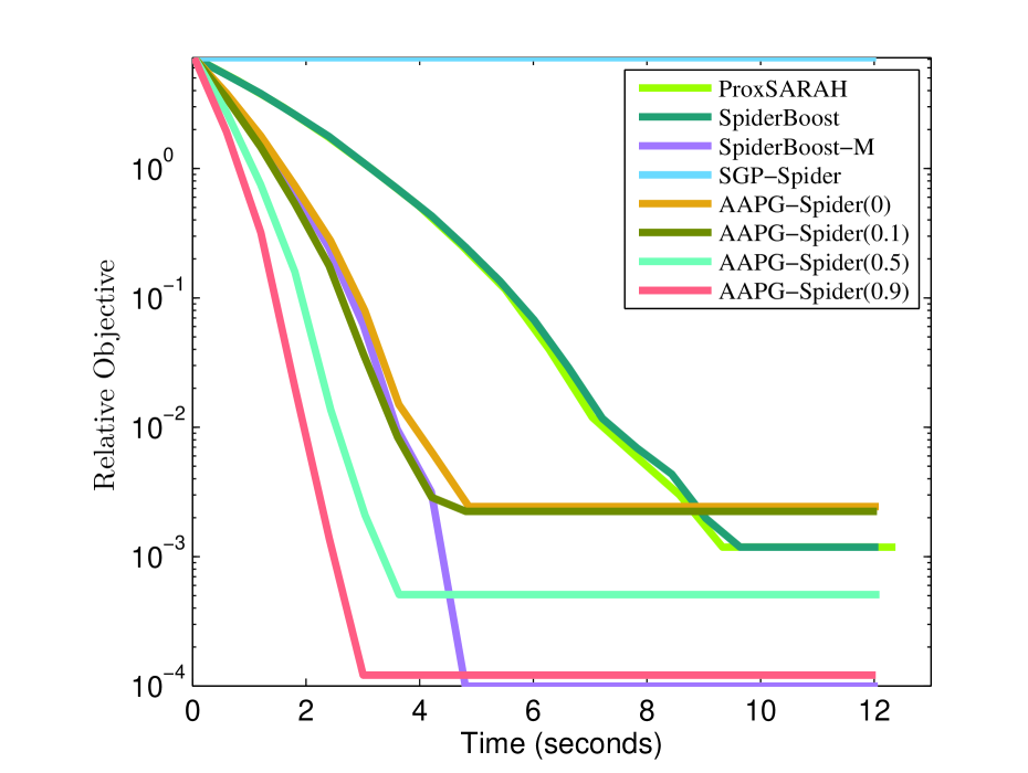
(a) cifar-10000-1000

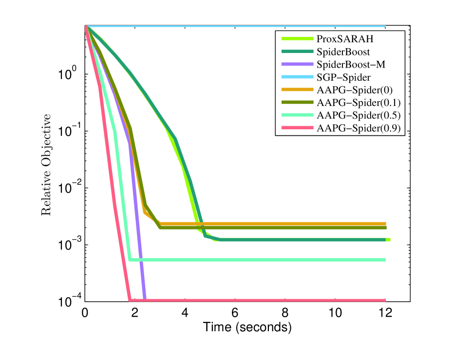
(b) gisette-5000-1000

(c) cnncaltech-3000-1000

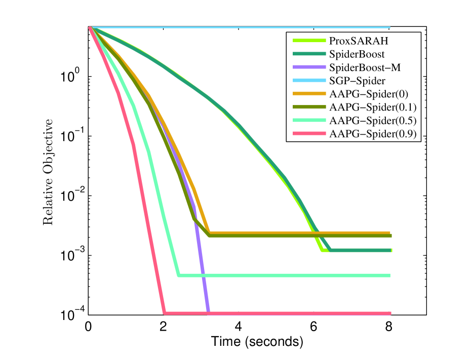
(d) randn-10000-1000

Figure 5: The convergence curve of the compared methods for sparse phase retrieval with $\dot{\lambda}=0.01$.

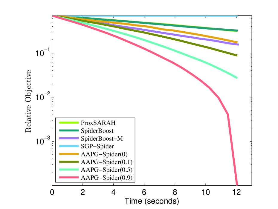
(e) cifar-10000-1000

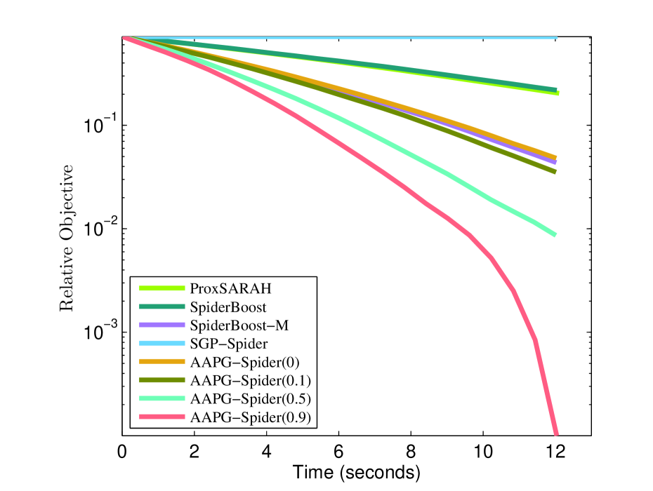
(f) gisette-5000-1000

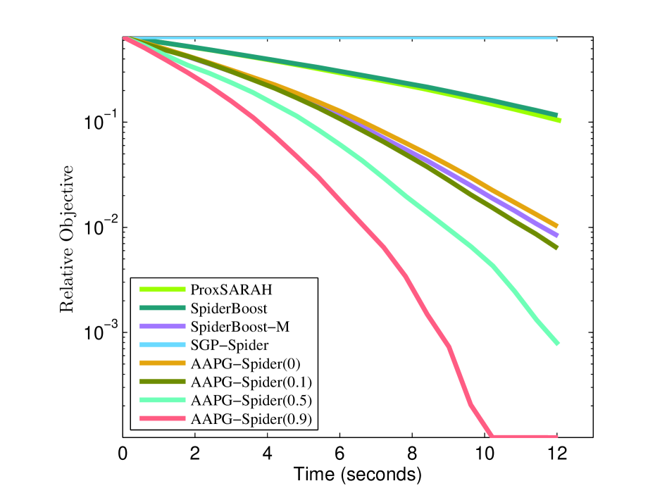
(g) cnncaltech-3000-1000

(h) randn-10000-1000

Figure 6: The convergence curve of the compared methods for sparse phase retrieval with $\dot{\lambda}=0.001$.

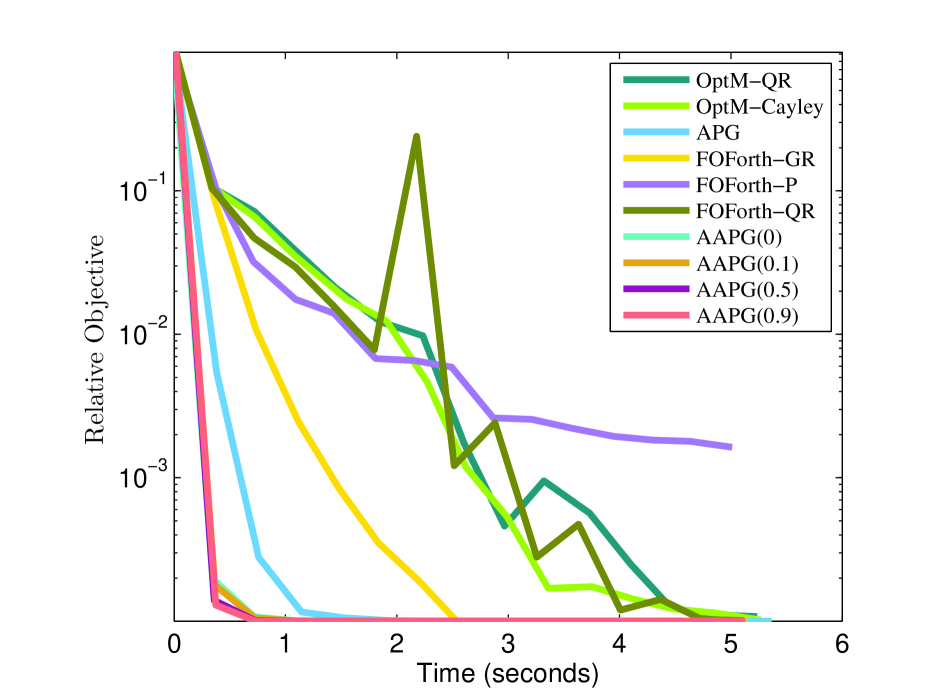
(a) cifar-5000-1000

(b) gisette-6000-3000

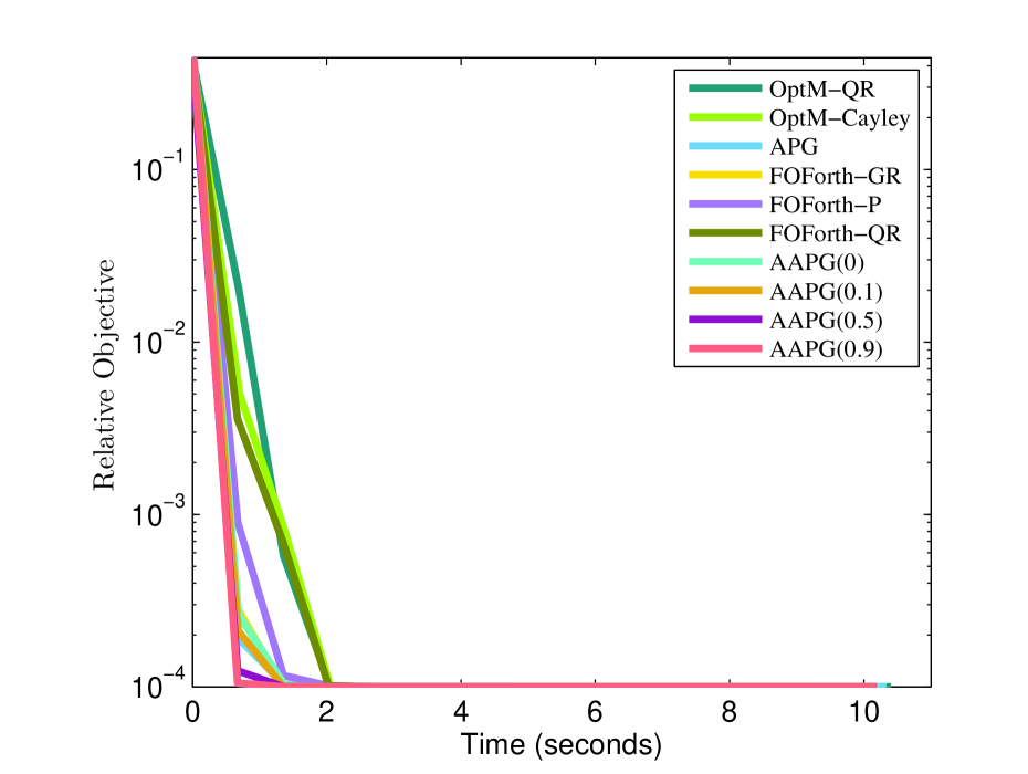
(c) cnncaltech-2000-1000

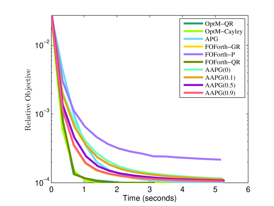
(d) randn-3000-1000

Figure 7: The convergence curve of the compared methods for linear eigenvalue problems with $\dot{r}=20$.

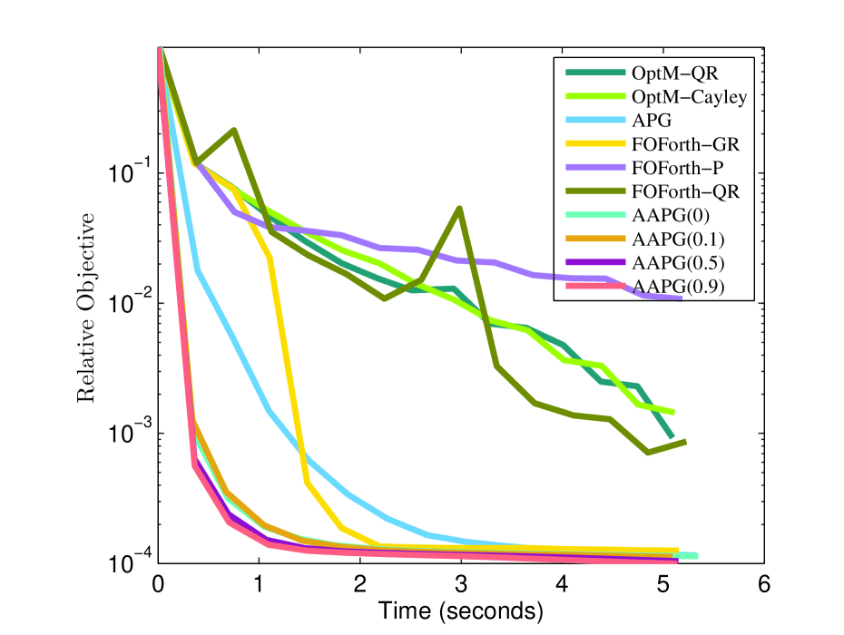
(a) cifar-5000-1000

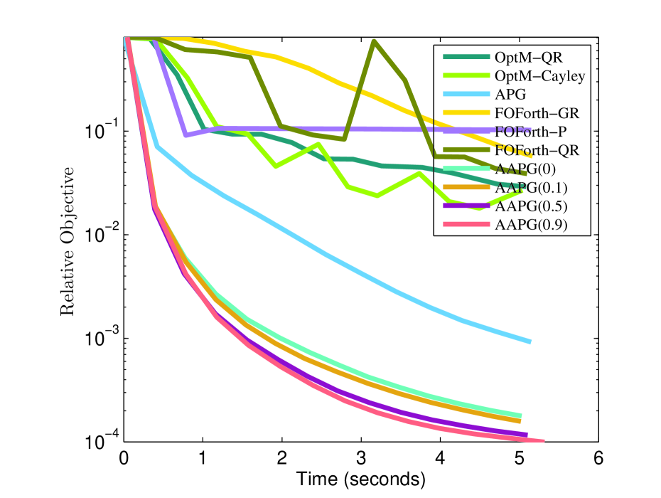
(b) gisette-6000-3000

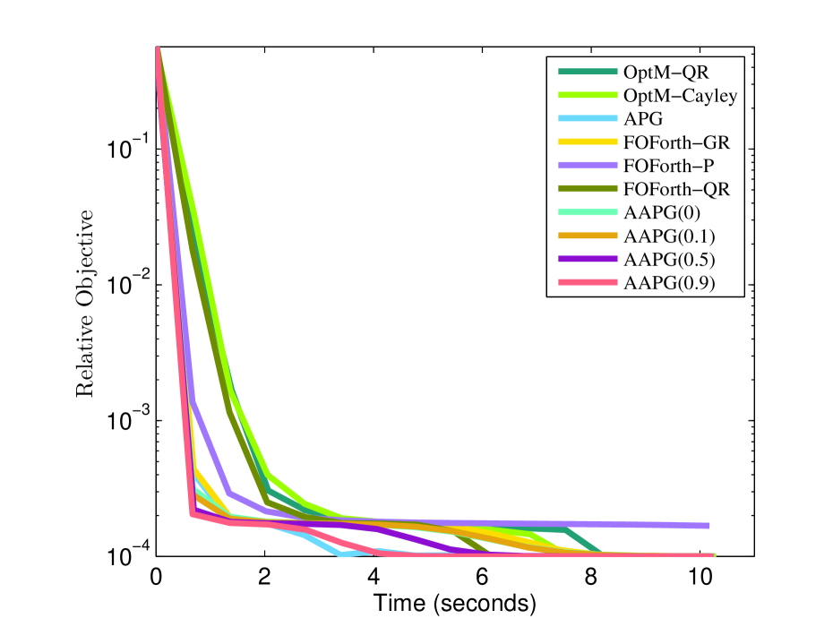
(c) cnncaltech-2000-1000

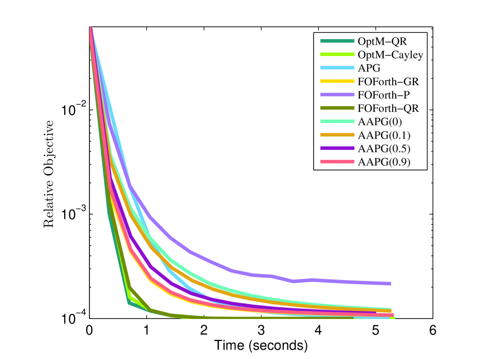
(d) randn-3000-1000

Figure 8: The convergence curve of the compared methods for linear eigenvalue problems with $\dot{r}=50$.

References

- Attouch & Bolte (2009) Attouch, H. and Bolte, J. On the convergence of the proximal algorithm for nonsmooth functions involving analytic features. Mathematical Programming, 116(1-2):5–16, 2009.
- Attouch et al. (2010) Attouch, H., Bolte, J., Redont, P., and Soubeyran, A. Proximal alternating minimization and projection methods for nonconvex problems: An approach based on the kurdyka-lojasiewicz inequality. Mathematics of Operations Research, 35(2):438–457, 2010.
- Bai et al. (2019) Bai, Y., Wang, Y., and Liberty, E. Proxquant: Quantized neural networks via proximal operators. In International Conference on Learning Representations (ICLR), 2019.
- Beck & Teboulle (2009) Beck, A. and Teboulle, M. A fast iterative shrinkage-thresholding algorithm for linear inverse problems. SIAM Journal on Imaging Sciences, 2(1):183–202, 2009.
- Bertsekas (2015) Bertsekas, D. Convex optimization algorithms. Athena Scientific, 2015.
- Bolte et al. (2014) Bolte, J., Sabach, S., and Teboulle, M. Proximal alternating linearized minimization for nonconvex and nonsmooth problems. Mathematical Programming, 146(1-2):459–494, 2014.
- Cai et al. (2024) Cai, J., Long, Y., Wen, R., and Ying, J. A fast and provable algorithm for sparse phase retrieval. In International Conference on Learning Representations (ICLR), 2024.
- Candes et al. (2008) Candes, E. J., Wakin, M. B., and Boyd, S. P. Enhancing sparsity by reweighted minimization. Journal of Fourier analysis and applications, 14:877–905, 2008.
- Chen et al. (2022) Chen, C., Shen, L., Zou, F., and Liu, W. Towards practical adam: Non-convexity, convergence theory, and mini-batch acceleration. Journal of Machine Learning Research, 23(229):1–47, 2022.
- Defazio & Mishchenko (2023) Defazio, A. and Mishchenko, K. Learning-rate-free learning by d-adaptation. In International Conference on Machine Learning (ICML), volume 202, pp. 7449–7479, 2023.
- Defazio et al. (2014) Defazio, A., Bach, F., and Lacoste-Julien, S. Saga: A fast incremental gradient method with support for non-strongly convex composite objectives. Advances in Neural Information Processing Systems (NeurlPS), 27, 2014.
- Duchi et al. (2011) Duchi, J., Hazan, E., and Singer, Y. Adaptive subgradient methods for online learning and stochastic optimization. Journal of Machine Learning Research, 12(7), 2011.
- Fang et al. (2018) Fang, C., Li, C. J., Lin, Z., and Zhang, T. Spider: Near-optimal non-convex optimization via stochastic path-integrated differential estimator. Advances in Neural Information Processing Systems (NeurlPS), 31, 2018.
- Gao et al. (2018) Gao, B., Liu, X., Chen, X., and Yuan, Y.-x. A new first-order algorithmic framework for optimization problems with orthogonality constraints. SIAM Journal on Optimization, 28(1):302–332, 2018.
- Geman & Yang (1995) Geman, D. and Yang, C. Nonlinear image recovery with half-quadratic regularization. IEEE transactions on Image Processing, 4(7):932–946, 1995.
- Ghadimi & Lan (2013) Ghadimi, S. and Lan, G. Stochastic first- and zeroth-order methods for nonconvex stochastic programming. SIAM Journal on Optimization, 23(4):2341–2368, 2013.
- Ghadimi & Lan (2016) Ghadimi, S. and Lan, G. Accelerated gradient methods for nonconvex nonlinear and stochastic programming. Mathematical Programming, 156(1):59–99, 2016.
- Ghadimi et al. (2016) Ghadimi, S., Lan, G., and Zhang, H. Mini-batch stochastic approximation methods for nonconvex stochastic composite optimization. Mathematical Programming, 155(1-2):267–305, 2016.
- J. Reddi et al. (2016) J. Reddi, S., Sra, S., Poczos, B., and Smola, A. J. Proximal stochastic methods for nonsmooth nonconvex finite-sum optimization. In Advances in Neural Information Processing Systems (NeurlPS), volume 29, 2016.
- Jiang & Stich (2024) Jiang, X. and Stich, S. U. Adaptive sgd with polyak stepsize and line-search: Robust convergence and variance reduction. Advances in Neural Information Processing Systems (NeurlPS), 36, 2024.
- Johnson & Zhang (2013) Johnson, R. and Zhang, T. Accelerating stochastic gradient descent using predictive variance reduction. In Advances in Neural Information Processing Systems, volume 26, 2013.
- Kavis et al. (2022a) Kavis, A., Levy, K. Y., and Cevher, V. High probability bounds for a class of nonconvex algorithms with adagrad stepsize. In International Conference on Learning Representations (ICLR), 2022a.
- Kavis et al. (2022b) Kavis, A., Skoulakis, S., Antonakopoulos, K., Dadi, L. T., and Cevher, V. Adaptive stochastic variance reduction for non-convex finite-sum minimization. Advances in Neural Information Processing Systems, 35:23524–23538, 2022b.
- Kingma & Ba (2015) Kingma, D. P. and Ba, J. Adam: A method for stochastic optimization. In International Conference on Learning Representations (ICLR), 2015.
- Li & Lin (2015) Li, H. and Lin, Z. Accelerated proximal gradient methods for nonconvex programming. Advances in Neural Information Processing Systems (NeurlPS), 28, 2015.
- Li et al. (2017) Li, Q., Zhou, Y., Liang, Y., and Varshney, P. K. Convergence analysis of proximal gradient with momentum for nonconvex optimization. In International Conference on Machine Learning (ICML), pp. 2111–2119, 2017.
- Li et al. (2023) Li, X., Milzarek, A., and Qiu, J. Convergence of random reshuffling under the kurdyka–lojasiewicz inequality. SIAM Journal on Optimization, 33(2):1092–1120, 2023.
- Li & Li (2018) Li, Z. and Li, J. A simple proximal stochastic gradient method for nonsmooth nonconvex optimization. Advances in Neural Information Processing Systems (NeurlPS), 31, 2018.
- Li et al. (2021) Li, Z., Bao, H., Zhang, X., and Richtarik, P. Page: A simple and optimal probabilistic gradient estimator for nonconvex optimization. In International Conference on Machine Learning (ICML), pp. 6286–6295, 2021.
- McMahan & Streeter (2010) McMahan, H. B. and Streeter, M. J. Adaptive bound optimization for online convex optimization. In Conference on Learning Theory (COLT), pp. 244–256, 2010.
- Mordukhovich (2006) Mordukhovich, B. S. Variational analysis and generalized differentiation i: Basic theory. Berlin Springer, 330, 2006.
- Nesterov (2003) Nesterov, Y. Introductory lectures on convex optimization: A basic course, volume 87. Springer Science & Business Media, 2003.
- Nguyen et al. (2017) Nguyen, L. M., Liu, J., Scheinberg, K., and Takac, M. Sarah: A novel method for machine learning problems using stochastic recursive gradient. In International Conference on Machine Learning (ICML), pp. 2613–2621, 2017.
- Oikonomidis et al. (2024) Oikonomidis, K., Laude, E., Latafat, P., Themelis, A., and Patrinos, P. Adaptive proximal gradient methods are universal without approximation. In International Conference on Machine Learning (ICML), volume 235, pp. 38663–38682, 2024.
- Pham et al. (2020) Pham, N. H., Nguyen, L. M., Phan, D. T., and Tran-Dinh, Q. Proxsarah: An efficient algorithmic framework for stochastic composite nonconvex optimization. Journal of Machine Learning Research, 21(110):1–48, 2020.
- Qian & Pan (2023) Qian, Y. and Pan, S. Convergence of a class of nonmonotone descent methods for kurdyka-lojasiewicz optimization problems. SIAM Journal on Optimization, 33(2):638–651, 2023.
- Rockafellar & Wets. (2009) Rockafellar, R. T. and Wets., R. J.-B. Variational analysis. Springer Science & Business Media, 317, 2009.
- Schmidt et al. (2013) Schmidt, M., Le Roux, N., and Bach, F. Minimizing finite sums with the stochastic average gradient. arXiv, 2013.
- Shechtman et al. (2014) Shechtman, Y., Beck, A., and Eldar, Y. C. Gespar: Efficient phase retrieval of sparse signals. IEEE Transactions on Signal Processing, 62(4):928–938, 2014.
- Sutskever et al. (2013) Sutskever, I., Martens, J., Dahl, G., and Hinton, G. On the importance of initialization and momentum in deep learning. In International Conference on Machine Learning (ICML), pp. 1139–1147, 2013.
- Wang et al. (2023) Wang, X., Johansson, M., and Zhang, T. Generalized polyak step size for first order optimization with momentum. In International Conference on Machine Learning (ICML), pp. 35836–35863. PMLR, 2023.
- Wang et al. (2019) Wang, Z., Ji, K., Zhou, Y., Liang, Y., and Tarokh, V. Spiderboost and momentum: Faster variance reduction algorithms. Advances in Neural Information Processing Systems (NeurlPS), 32, 2019.
- Ward et al. (2020) Ward, R., Wu, X., and Bottou, L. Adagrad stepsizes: Sharp convergence over nonconvex landscapes. Journal of Machine Learning Research, 21(219):1–30, 2020.
- Wen & Yin (2013) Wen, Z. and Yin, W. A feasible method for optimization with orthogonality constraints. Mathematical Programming, 142(1-2):397, 2013.
- Yang (2023) Yang, L. Proximal gradient method with extrapolation and line search for a class of non-convex and non-smooth problems. Journal of Optimization Theory and Applications, 200(1):68–103, 2023.
- Yang et al. (2020) Yang, Y., Yuan, Y., Chatzimichailidis, A., van Sloun, R. J., Lei, L., and Chatzinotas, S. Proxsgd: Training structured neural networks under regularization and constraints. In International Conference on Learning Representations (ICLR), 2020.
- Yun et al. (2021) Yun, J., Lozano, A. C., and Yang, E. Adaptive proximal gradient methods for structured neural networks. Advances in Neural Information Processing Systems (NeurlPS), 34:24365–24378, 2021.
- Zhang (2010a) Zhang, C.-H. Nearly unbiased variable selection under minimax concave penalty. The Annals of Statistics, pp. 894–942, 2010a.
- Zhang et al. (2019) Zhang, G., Wang, C., Xu, B., and Grosse, R. B. Three mechanisms of weight decay regularization. In International Conference on Learning Representations (ICLR), 2019.
- Zhang (2010b) Zhang, T. Analysis of multi-stage convex relaxation for sparse regularization. Journal of Machine Learning Research, 11(3), 2010b.
- Zhou et al. (2020) Zhou, D., Xu, P., and Gu, Q. Stochastic nested variance reduction for nonconvex optimization. The Journal of Machine Learning Research, 21(1):4130–4192, 2020.
- Zhou et al. (2024) Zhou, D., Ma, S., and Yang, J. Adabb: Adaptive barzilai-borwein method for convex optimization. arXiv preprint arXiv:2401.08024, 2024.