Deep learning-based filtering of cross-spectral matrices using generative adversarial networks ††thanks: This research has been funded by German Federal Ministry for Economic Affairs and Climate Action (Bundesministerium für Wirtschaft und Klimaschutz BMWK) under project AntiLerM registration number 49VF220063.
Abstract
In this paper, we present a deep-learning method to filter out effects such as ambient noise, reflections, or source directivity from microphone array data represented as cross-spectral matrices. Specifically, we focus on a generative adversarial network (GAN) architecture designed to transform fixed-size cross-spectral matrices. Theses models were trained using sound pressure simulations of varying complexity developed for this purpose. Based on the results from applying these methods in a hyperparameter optimization of an auto-encoding task, we trained the optimized model to perform five distinct transformation tasks derived from different complexities inherent in our sound pressure simulations.
Index Terms:
Deep learning, cross-spectral matrix, GAN.I Introduction
As extensively investigated in [5], state-of-the-art deep-learning methods for acoustical sound source localization (SSL) aim to directly reconstruct the direction of arrival of sources or, more generally, the parameters describing the acoustic scene in the presence of reverberation or diffuse noise. This article addresses the problem from a different perspective by employing generative adversarial networks (GANs) to either remove or, at least, reduce the effects of ambient noise, reflections, or source directivity in microphone array data (that is, cross-spectral matrices) before any potential SSL analysis begins. On the one hand, this approach improves the starting point for solving the SSL problem, on the other hand, it enables a more effective use of traditional mapping methods such as standard beamforming or CLEAN-SC.
II Acoustic simulations
II-A Basics
Let be the complex amplitude of a time-harmonic sound pressure field of angular frequency and speed of propagation . By definition, satisfies the Helmholtz equation
| (1) |
Our sign convention for a time-harmonic function is . For example,
| (2) |
represents an outgoing spherical wave with source in .
Let be ’s representation in spherical coordinates . Solutions to the corresponding Helmholtz equation can be found analytically by assuming that is separable, i.e. there exist functions , , such that
| (3) |
In this case, the Helmholtz equation leads necessarily to
| (4) |
for some constants , , and , denote the spherical Hankel functions of the first and second kind of degree , respectively. Moreover, we have
| (5) |
where , and is the spherical harmonic of degree and order .
II-B Smooth spherical pistons
A vibrating spherical cap piston with aperture angle centered on the north pole of an otherwise rigid sphere with radius can be described by its surface velocity ,
| (6) |
the corresponding aperture function is given by
| (7) |
The spherical wave spectrum of ,
| (8) |
can be computed via integration of the corresponding associated Legendre polynomials:
| (9) |
Rotating the spherical cap to be centered in the direction results in
| (10) |
respectively. Finally, the radiated pressure in the region is completely determined by the surface velocity spectrum (see for example [11]):
| (11) |
As most of the higher degrees in (8) are present to form the discontinuity at the boundary of the spherical cap, we opt for a smooth one-parameter family of spherical pistons as fundamental building block of our acoustical models. Its surface velocity is defined via
| (12) |
Again, we will call the aperture angle of this piston, but now, when varying from to , the particle velocity smoothly changes from to in the case . As before, the spherical wave spectrum of can be determined by one-dimensional integration,
| (13) |
where . Moreover, transformation rule (10) also holds for the coefficients when rotating the smooth spherical piston to be centered in the direction , and the radiated sound pressure corresponding to can be computed in complete analogy to (11).
II-C Acoustic models
The simulations involved a set of acoustic models fixed beforehand and each consisting of three (outgoing) smooth spherical pistons which were rotated and translated uniformly at random along the plane within a cube of edge length that is centered at the origin. Moreover, each source is furnished with its own reflection plane together with a reflection coefficient between and . The aperture angles of the pistons vary from to (acoustic monopole) and source radii are chosen randomly and uniformly between and . Within each model, the source ’s are chosen to be at most below the model sound velocity level, which ranges uniformly between and across the model set. Consequently, the maximum dynamic range between sources within each model is . Model temperatures are taken from a normal distribution with a mean of and a standard deviation of .
We approximated the sound pressures of these models up to Helmholtz degree at the positions of a virtual microphone array of spherical shape ( microphones, diameter , centered at with ) for distinct frequencies:
| (14) |
In this process, each source of the model set was furnished with its own spectral distribution function ,
| (15) |
where the center frequency was ranging uniformly from to , and the frequency width parameter was chosen between and , again, uniformly at random.
Finally, we included an arbitrary pressure field of degree (incoming towards the origin) to model ambient sound. The upper bound for the magnitude of the corresponding randomly chosen complex coefficients is given by
| (16) |
where is at least below the model sound velocity level.
III Machine learning model
III-A Generative Adversarial Networks
The machine learning model we present below is based on a GAN architecture (see [4]), where, when training the model, a pass through the learning loop can be interpreted as a round of a zero-sum game in the sense of game theory. Here, the two players, generator and discriminator, confront each other and aim to optimize their respective objective functions. More precisely, the generator and discriminator are artificial neural networks whose parameters are optimized according to loss functions derived from their respective objective functions.
In general, the generator is a mapping between spaces and , where , on the one hand, contains the set of training data (also referred to as real data) and, on the other hand, defines what is considered to be achievable through generation: the elements of the image are called the fake data generated by from . For example, in what follows, , therefore, it contains the cross-spectral matrices built from our sound pressure simulations in II-C.
Now, the discriminator is a mapping from to the unit interval. In each pass through the learning loop, a finite set of training data is drawn randomly (this is also called mini-batching approach [3]) and complemented by a finite set of realizations of a random variable with a fixed probability distribution taking values in . The goal of the discriminator is now to distinguish between the real data and the fake data generated from . More specifically, is optimized according to the loss function
| (17) |
where denotes the natural logarithm. On the opposite side, the objective of the generator is to make the fake data generated from appear as real as possible from the discriminator’s point of view. This is achieved by optimizing the parameters of using the loss function
| (18) |
In summary, through this adversarial process, both networks are optimized to improve their respective capabilities in processing the training data (see [8]).
III-B Complex model building blocks
As the ability to take into account phase information will be crucial when working with cross-spectral matrices, all building blocks of the deep neural networks that follow will be real representations of complexifications of their traditional real-valued counterparts (see [9]): Suppose is a real matrix representation of a linear network operation, where is the corresponding vector of learnable parameters. Then, simply by switching to the field of complex numbers, we deduce that for satisfies
| (19) | ||||
| (20) |
for all . Therefore, we will call
| (21) |
a real matrix representation of the complexification of the network operation of .
In addition to linear network operations, we make use of two complex phase-preserving activation functions in order to build networks that represent non-linear complex functions. Firstly, we employ a so-called modified ReLU activation function with bias , which is defined as follows (see [1]):
| (22) | ||||
| (23) |
And secondly, we apply a leaky variant ,
| (24) |
of the complex cardioid activation function of [10]. The absolute value of the latter depends on the phase of , whereas the former does not.
III-C Models for generator and discriminator
The generator we are going to employ is a composition of two convolutional neural networks, encoder and decoder . The input of the encoder takes values of , hence, it can be applied to cross-spectral matrices built out of the simulations of II-C. The kernel of the utilized (transposed) two-dimensional complex bias-free convolutions is with trivial stride. Therefore, a padding strategy was not necessary. The encoder is composed of one such convolutional layer and one to four complex bias-free dense layers (cf. III-B),
| (25) |
Here, every convolution or dense layer entails an activation using one of the functions of III-B,
| (26) |
is an alternative notation for , the number of convolution filters is , and the number of dense units is . The decoder realizes
| (27) |
( denotes transposed convolution) followed by a Hermitianizing operation ,
| (28) |
The discriminator is similar in structure to the encoder, but with removed dense layers, and the number of convolution filters now is :
| (29) |
Moreover, a real sigmoid activation function is applied the real and the imaginary parts of the convolution output (a so-called split-type A activation, see [2]), and the corresponding result is averaged over all dimensions of its real representation.
III-D Training set and loop
Following the notation of III-A, we now fix
| (30) |
Moreover, we decide on a transformation rule the generator is intended to learn (cf. IV-B). More precisely, we decide on sets and and a map . For example, in the most trivial case, could be trained to work as an auto-encoder on a fixed set by setting and .
In each pass through the training loop, and is generated out of and (with being a mini-batch drawn randomly from , and , see III-A) by adding noise, respectively. Based on III-A, we add another term to to integrate the transformation rule intended for ,
| (31) | ||||
| (32) |
Here, , ,
| (33) |
| (34) | ||||
| (35) |
, . Moreover, denotes the Frobenius norm and is the projection onto the -th component,
| (36) |
To summarize (31) and (32), is sought to be a denoising opponent to the discriminator that, on the one hand, realizes the map on elements of , and, on the other hand, is an auto-encoder for the elements of .
IV Results
IV-A Hyperparameter optimization
Some of the parameters involved in the training process were chosen based on preliminary experiments or computational limitations. For example, we fixed the mini-batch size to be , and the size of the training data set was chosen as . Moreover, each component of was normalized with respect to its Frobenius norm as a preprocessing step after the pressure simulations of II-C. As a consequence, we were able to balance (31) and (32) in terms of their magnitude by setting . For the stochastic gradient descent of generator and discriminator, we used Adam optimizers with , , without exponential moving average (see [7]).
The remaining parameters were chosen in a hyperparameter optimization. As metric to assess the quality of this optimization, we opted for the average accuracy
| (37) |
on a test data set of elements disjoint to using our weighted distance function (see (33)) that utilizes the correlation matrix distance of [6]. The parameter combinations that were tested included the number of convolution filters in the generator and the discriminator , the number of dense units and dense layers in the encoder and decoder, the learning rates of the Adam optimizers for generator and discriminator, and the used activation function: with or with . The combination
| (38) | ||||
| (39) |
together with , yielded the maximum value of after epochs of training using and (more specifically, task 1) in IV-B).
IV-B Transformation tasks
After hyperparameter optimization, we investigated transformation tasks was intended to learn. For each of these tasks, we started by selecting a set of models from our model set we presented in II-C. We then simulated each of these models in two different complexities creating and . The latter built up and , respectively, and we set . We considered the following pairings:
-
1)
Auto-encoder pairing,
-
2)
exhibits ambient sound, does not
-
3)
exhibits reflections, does not
-
4)
exhibits directivity, does not
-
5)
exhibits directivity, reflections and ambient sound, none of these
If not stated otherwise here, a model was simulated with monopole sources, without reflections and with no ambient sound present.
After epochs of training, we tested the resulting generator by reiterating the previous steps for a model set disjoint to , . For each element of the corresponding set , we evaluated
| (40) |
and (see (37)) is simply the average of these results,
| (41) |
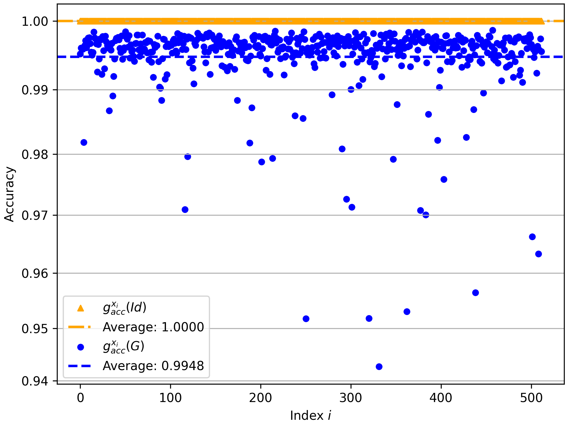
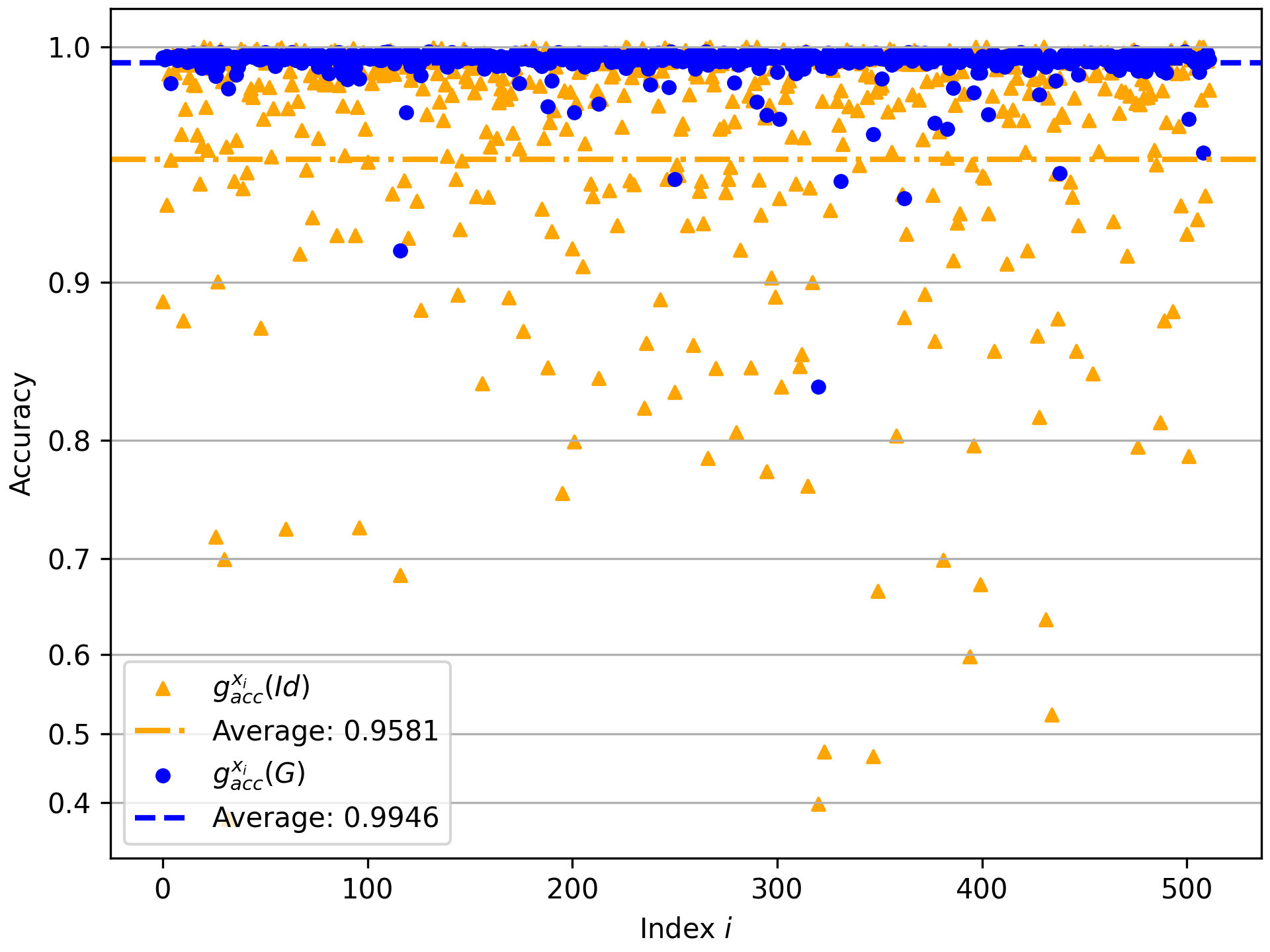
For example, the results of the auto-encoder transformation task 1) can be found in fig. 1. The average accuracy was in this case serving as baseline, as the corresponding results of all other cases are expected to be lower or equal. In addition, we place these values side-by-side with and its average , respectively, in order to quantify the initial situation in comparison for all transformation tasks (see figs. 1-5).
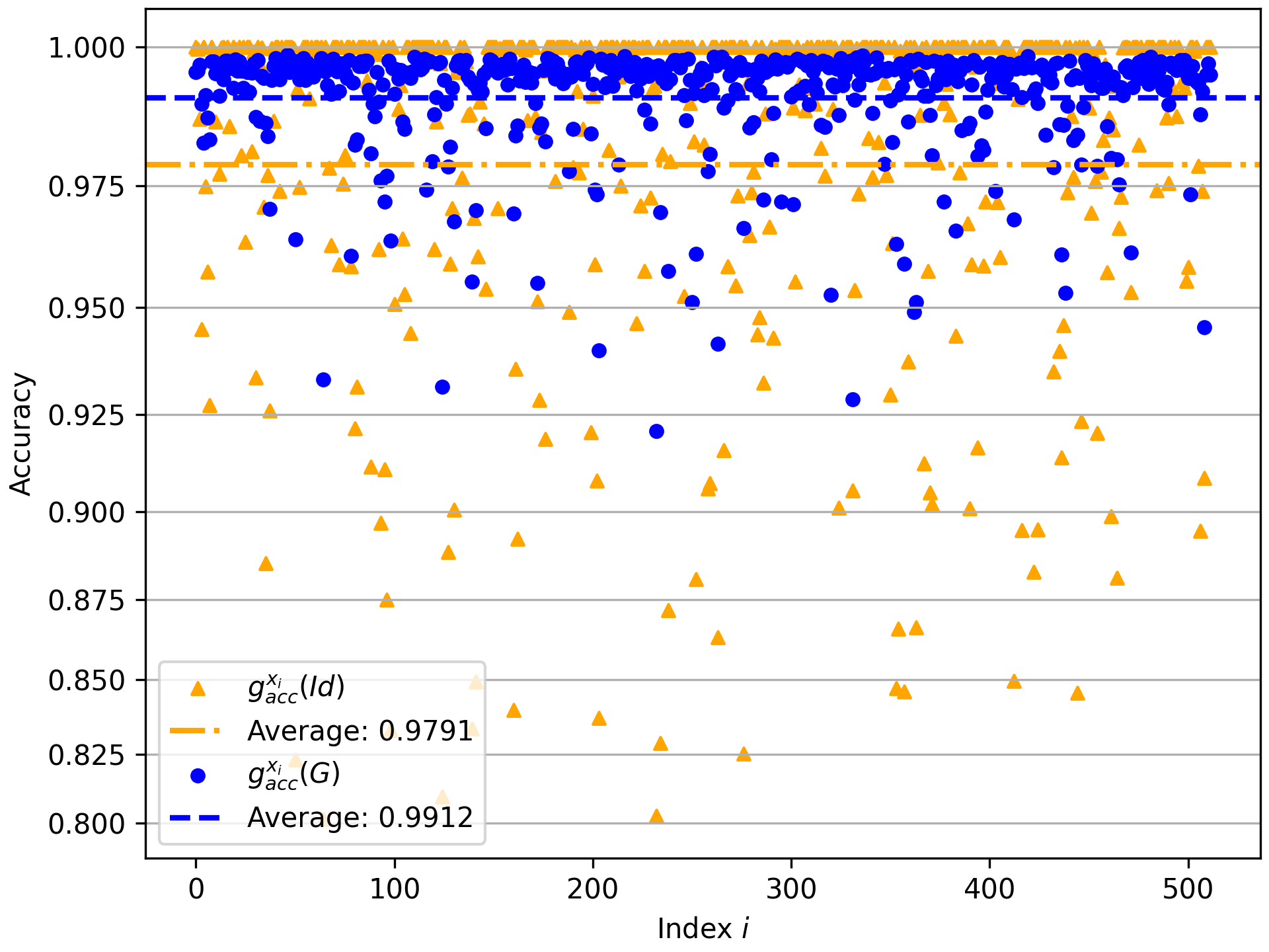
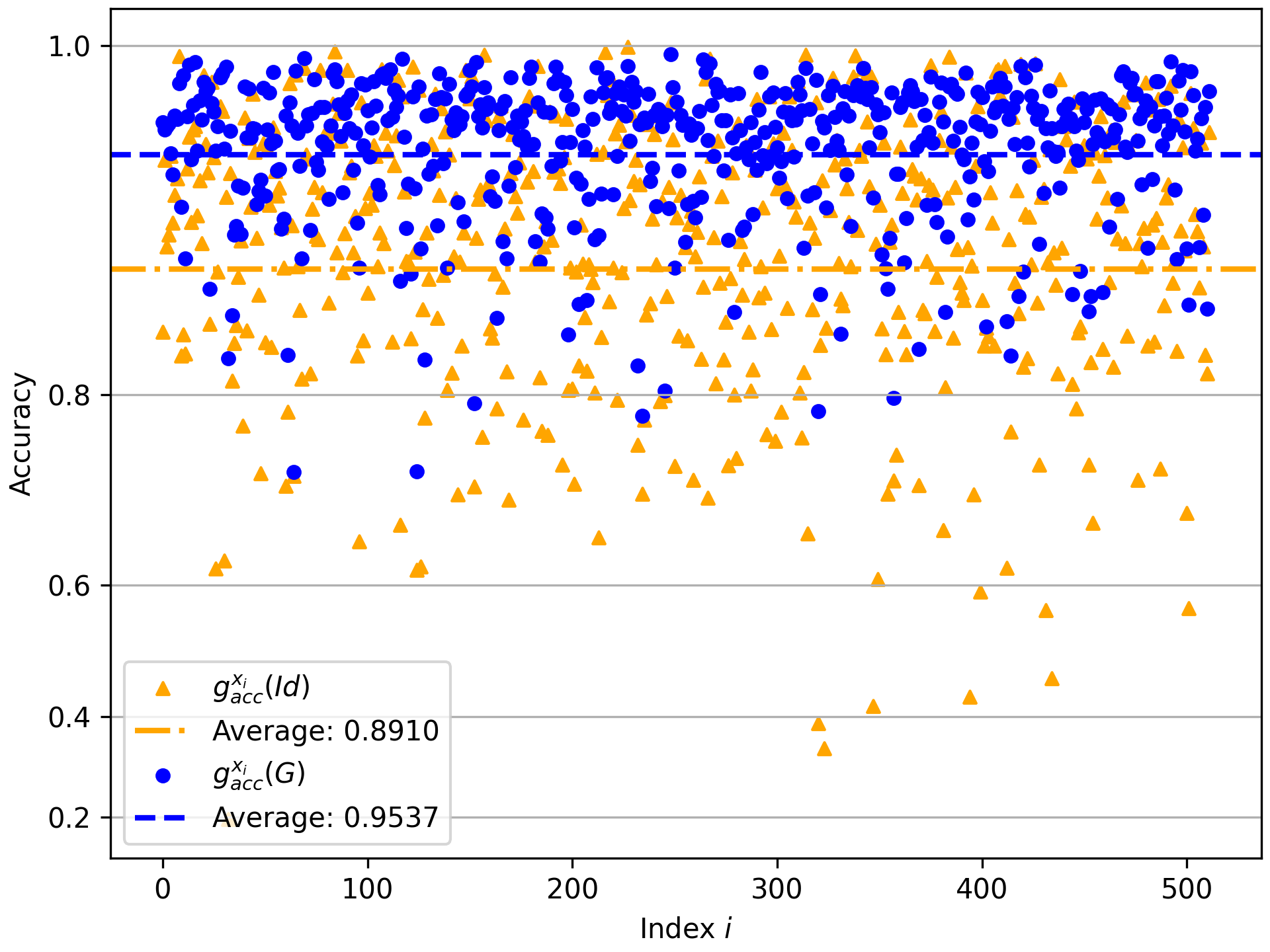
The lowest resulting values were achieved in cases 4) and 5) where the corresponding transformation task included to remove the directivity information from the data. This could be expected as the microphone array used in the simulations was only of small aperture compared to size of the total acoustic scene. Moreover, when analyzing as a function of learning epoch, it became clear, that the training progress was much slower and did not converge within epochs of training in the cases 4) and 5). Studying fig. 3 more carefully, we realize that there are many models with for transformation task 3). This is due to the fact that although a reflection plane was present, its position did not render a reflection possible.

References
- [1] M. Arjovsky, A. Shah, and Y. Bengio, “Unitary evolution recurrent neural networks,” Proceedings of the 33rd International Conference on Machine Learning (ICML’16), 2016.
- [2] J. Bassey, “A Survey of Complex-Valued Neural Networks,” 2021, arXiv:2101.12249. [Online]. Available: https://arxiv.org/abs/2101.12249.
- [3] L. Bottou: “Online Algorithms and Stochastic Approximations,” Cambridge University Press, 1998.
- [4] I. J. Goodfellow, J. Pouget-Abadie, M. Mirza, B. Xu, D. Warde-Farley, S. Ozair, A. Courville, and Y. Bengio, “Generative Adversarial Nets,” Proceedings of the 27th International Conference on Neural Information Processing Systems (NIPS 2014), 2014.
- [5] P.-A. Grumiaux, S. Kitić, L. Girin, and A. Guérin, “A survey of sound source localization with deep learning methods,” J. Acoust. Soc. Am. 152, 107–151, 2022.
- [6] M. Herdin, N. Czink, H. Ozcelik, and E. Bonek, “Correlation matrix distance, a meaningful measure for evaluation of non-stationary MIMO channels ,” Proceedings of the 2005 IEEE 61st Vehicular Technology Conference (VETECS 2005), 2005.
- [7] D. Kingma, and J. L. Ba, “Adam: A Method for Stochastic Optimization,” Proceedings of the 3rd International Conference for Learning Representations (ICLR 2015), 2015.
- [8] T. Salimans, I. Goodfellow, W. Zaremba, V. Cheung, A. Radford, and X. Chen, “Improved techniques for training GANs,” Advances in Neural Information Processing Systems 29 (NIPS 2016), 2016.
- [9] C. Trabelsi, O. Bilaniuk, Y. Zhang, D. Serdyuk, S. Subramanian, J. F. Santos, S. Mehri, N. Rostamzadeh, Y. Bengio, and C. J. Pal, “Deep Complex Networks,” Proceedings of the 6th International Conference on Learning Representations (ICLR 2018), 2018.
- [10] P. Virtue, X. Y. Stella, and M. Lustig, “Better than real: complex-valued neural nets for MRI fingerprinting,” Proceedings of the 2017 IEEE International Conference on Image Processing (ICIP 2017), 2017.
- [11] E. G. Williams, “Fourier acoustics: sound radiation and nearfield acoustical holography,” Academic Press, 1999.