System Identification Beyond the Nyquist Frequency: A Kernel-Regularized Approach

Abstract

Models that contain intersample behavior are important for control design of systems with slow-rate outputs. The aim of this paper is to develop a system identification technique for fast-rate models of systems where only slow-rate output measurements are available, e.g., vision-in-the-loop systems. In this paper, the intersample response is estimated by identifying fast-rate models through least-squares criteria, and the limitations of these models are determined. In addition, a method is developed that surpasses these limitations and is capable of estimating unique fast-rate models of arbitrary order by regularizing the least-squares estimate. The developed method utilizes fast-rate inputs and slow-rate outputs and identifies fast-rate models accurately in a single identification experiment. Finally, both simulation and experimental validation on a prototype wafer stage demonstrate the effectiveness of the framework.

[1]organization=Department of Mechanical Engineering, Control Systems Technology Section, Eindhoven University of Technology, addressline=Groene Loper 5, city=Eindhoven, postcode=5612 AE, country=The Netherlands. [2]organization=Automatic Control Laboratory, ETH Zürich, city=Zürich, postcode=8092, country=Switzerland. [3]organization=Delft Center for Systems and Control, Delft University of Technology, addressline=Mekelweg 2, city=Delft, postcode=2628 CN, country=The Netherlands.

1 Introduction

Systems which have their outputs sampled at a reduced sampling rate compared to their inputs are becoming more prevalent, particularly in applications such as vision-in-the-loop systems [1]. Slow-rate output measurements generally constrain the models to reflect only slow system dynamics. Unlike models that only reflect slow system dynamics, fast-rate models capture higher-frequency behavior, even beyond the Nyquist frequency. This enables monitoring intersample performance variables [2, 3] and control design [4].

System identification plays an essential role in understanding and modeling the dynamic behavior of systems for the use in control design. System identification finds broad application in areas such as digital twin creation [5] and control design [6]. Two distinct approaches are non-parametric and parametric system identification. Non-parametric system identification techniques, such as Frequency Response Functions (FRFs) [7], model systems without requiring a predefined structure. Unlike non-parametric approaches, parametric system identification generally involves a fixed model structure, e.g., using prediction error methods [8, 9]. A key development in system identification involves the application of kernel methods [10]. The unique properties of kernels offer a major advantage by enforcing high-level properties on the identified models, that in addition enable the identification of continuous-time models [11]. The high-level properties that are enforced by kernels include for example exponential decay and correlation of impulse response coefficients. For linear time-invariant equidistantly sampled systems, both parametric and non-parametric system identification techniques have been proven to work effectively.

Important developments have been made in identifying fast-rate models from slow-rate outputs, primarily in terms of continuous-time and low-order parametric identification. First, continuous-time identification aims to identify a parametric continuous-time model using input-output data, as outlined in Unbehauen1990 [12]. Typically, these methods require intersample assumptions on the input signals, e.g., zero-order hold or band-limited signals [13], and hence, do not utilize broadband fast-rate inputs. Second, several methods are developed for fast-rate parametric model identification using slow-rate methods, including methods for identification of low-order Finite Impulse-Response (FIR) [14] and output-error [15] models. Subspace [16] or hierarchical identification techniques [17], which identify a lifted system representation, are also developed. Generally, these methods aim to identify a low-order fast-rate model using slow-rate outputs by incorporating prior information through a certain model structure, which does not include non-parametric model structures.

A key development in non-parametric identification for fast-rate models using slow-rate outputs incorporates prior information through a local smoothness assumption on the frequency response [18]. The smoothness assumption allows one to disentangle aliased components in the frequency-domain. However, the local smoothness assumption is an approximation, since it assumes that the system can be approximated as a polynomial of a certain degree in the frequency domain, leading to a bias-variance trade-off [7, Section 7.2.6].

Although methods to identify fast-rate models using slow-rate measurements have been developed for certain scenarios, current approaches are limited to specific cases, including low-order parametric modeling and frequency-domain approaches. The aim of this paper is to present a general framework to identify non-parametric fast-rate models using slow-rate outputs, enabling more generic prior information. The developed method utilizes regularized estimators, which have been proven to work effectively in system identification for equidistantly sampled systems [10]. Specifically, system properties are enforced through the use of regularization or kernel techniques, expressed in either the frequency domain, similarly to Lataire2016 [19] and Hallemans2022 [20], or the time domain, that is illustrated in this paper. Compared to earlier regularized system identification approaches, the developed approach uniquely combines and utilizes slow-rate outputs, fast-rate inputs, and prior information of the system to identify fast-rate non-parametric models using slow-rate outputs. The key contributions are the following.

• Analysis of conditions for unique identification of fast-rate FIR models using slow-rate outputs, which are critical for practical applications (Section 3).

• Identification of arbitrary order fast-rate models using slow-rate outputs, including non-parametric models, by incorporating prior information through kernel regularization (Section 4).

• Validation of the framework for identification of fast-rate models for systems with slow-rate outputs using a simulation and an experimental setup consisting of a prototype wafer stage (Section 5 and Section 6).

Notation

Fast-rate and slow-rate signals are denoted by subscript $h$ and $l$, with sampling times and frequencies $T_{h}=\frac{1}{f_{h}}$ and $T_{l}=FT_{h}=\frac{1}{f_{l}}$, with downsampling factor $F\in\mathbb{Z}_{>0}$ and integers $\mathbb{Z}$, discrete-time indices $n\in\mathbb{Z}_{[0,N-1]}$ and $m\in\mathbb{Z}_{[0,M-1]}$, with $N,M$ being the number of samples. Fast-rate and slow-rate discrete Fourier transforms are denoted with

$$X_{h}(e^{j\omega_{k}T_{h}}) =\sum_{n=0}^{N-1}x_{h}(n)e^{-j\omega_{k}T_{h}n},$$ (1)

$$X_{l}(e^{j\omega_{k}T_{l}}) =\sum_{m=0}^{M-1}x_{l}(m)e^{-j\omega_{k}T_{l}m},$$

with complex variable $j=\sqrt{-1}$, frequency grid $\omega_{k}=2\pi\frac{k}{N}f_{h}=2\pi\frac{k}{M}f_{l}$, and frequency bins $k\in\mathbb{R}$. The fast-rate forward shift operator is denoted by $q$, i.e., $q^{-1}x_{h}(n)=x_{h}(n-1)$. The Kronecker product is denoted with $\otimes$.

2 Problem Formulation

In this section, the considered problem is presented. The identification setting and identifiability problem associated to fast-rate models using slow-rate outputs are illustrated. Finally, the problem addressed in this paper is defined.

2.1 Identification Setting

The goal is to identify fast-rate model $G$ using slow-rate outputs $y_{l}(m)=\mathcal{S}_{d}y_{h}(n)=y_{h}(mF)$ and fast-rate inputs $u_{h}$, having sampling rates $f_{l}$ and $f_{h}=Ff_{l}$ and known downsampler $\mathcal{S}_{d}$. The open-loop identification setting is visualized in Figure 1.

Figure 1: Identification setup for systems with slow-rate output measurements.

The true fast-rate system $G_{0}$ is a linear time-invariant, single-input single-output system, and is described using the causal discrete-time state-space equations

$$G_{0}:\>\>\begin{cases}{x}(n+1)&=Ax(n)+Bu_{h}(n),\\ y_{h}(n)&=Cx(n)+Du_{h}(n).\end{cases}$$ (2)

The output is disturbed with zero-mean, independent, and identically distributed noise $e_{h}$, with variance $\sigma^{2}$, and downsampled into

$$y_{l}(m)=\mathcal{S}_{d}\left(y_{h}(n)+e_{h}(n)\right)=y_{h}(mF)+e_{h}(mF).$$ (3)

2.2 Identifiability of Fast-Rate Models

In this section, identifiability of fast-rate models for systems with slow-rate outputs is investigated. The system $G_{0}$ is modeled using the FIR filter $G(q,\theta)$, which has fast-rate model output

$$\hat{y}_{h}(n)=G(q,\theta)u_{h}(n)=\sum_{i=0}^{P-1}\theta_{i}q^{-i}u_{h}(n),$$ (4)

with model order $P\in\mathbb{Z}_{[1,N]}$, and FRF

$$G(e^{j\omega_{k}T_{h}})=\sum_{i=0}^{N-1}\theta_{i}e^{-j\omega_{k}T_{h}i}.$$ (5)

Similarly to (3), the slow-rate model output is downsampled as $\hat{y}_{l}(m)=\mathcal{S}_{d}\hat{y}_{h}(n)=\hat{y}_{h}(mF)$.

Identifiability of fast-rate models essentially involves determining whether the fast-rate input and the model structure allow for distinguishing between parameter values given the slow-rate output, which relates closely to the definition in Ljung1994 [21]. Specifically, the fast-rate input should be sufficiently informative to distinguish between different parameter sets $\theta$. Additionally, the model structure $G(q,\theta)$ should allow for distinguishing between different parameter sets $\theta$, provided a sufficiently informative input. The identifiability of fast-rate models is defined in Definition 1.

Definition 1.

The FIR coefficients $\theta$ of fast-rate model $G(q,\theta)$ in (4) are identifiable from slow-rate outputs if

$$\mathcal{S}_{d}G(q,\theta)u_{h}(n)=\mathcal{S}_{d}G(q,\theta^{*})u_{h}(n),\quad\Rightarrow\theta=\theta^{*}.$$ (6)

Fast-rate models are not always identifiable from slow-rate outputs, where several examples are illustrated in Example 1.

Example 1.

Consider the model structure $G\left(q,\theta\right)$ (4) for three parameter values $\theta$, $\theta^{*}$, and $\theta^{\prime}$ with order $P=1000$. Let $u_{h}$ be a fast-rate impulsive input with $N=P=1000$ samples, being persistently exciting of order $P=N$ [9, Lemma 13.1]. After downsampling by $F=4$, resulting in $M=250$ samples in the slow-rate output $y_{l}$, the responses of the three models are identical, i.e.,

$$\mathcal{S}_{d}G(q,\theta)u_{h}(n)=\mathcal{S}_{d}G(q,\theta^{*})u_{h}(n)=\mathcal{S}_{d}G(q,\theta^{\prime})u_{h}(n),$$

as illustrated in the top of Figure 2. However, these are generated by different fast-rate models, as highlighted by the fast-rate FRFs and impulse response coefficients in the bottom of Figure 2, indicating that the model is not identifiable according to Definition 1.

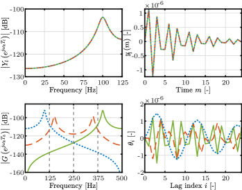
Figure 2: A non-identifiable model structure $G(q,\theta)$ for three specific impulse response coefficients $\theta$ ( ), $\theta^{*}$ ( ), and $\theta^{\prime}$ ( ) (bottom right), shown by their equal downsampled ouput in time-domain $\hat{y}_{l}$ (top right) and frequency-domain $\widehat{Y}_{l}\left(e^{jk\omega_{k}T_{l}}\right)$ (top left) for impulsive input $u_{h}$.

2.3 Problem Definition and Approach

The fast-rate model $G(q,\theta)$ from (4) is not always identifiable from slow-rate outputs given an arbitrary model order $P$ and fast-rate inputs $u_{h}$, as illustrated by Example 1.

The problem considered in this paper is as follows. Given the fast-rate input signal $u_{h}$ containing $N$ samples and slow-rate output $y_{l}$ containing $M$ samples, determine a fast-rate model $G(q,\theta)$ of order $P\in\mathbb{Z}_{[1,N]}$, and hence, includes non-parametric models with $P=N$, by incorporating appropriate prior information of the system.

3 Identification of Slow-Rate Systems

In this section, reduced-order FIR models are determined using a least-squares cost function, and several limitations thereof are shown, thereby constituting contribution C1. Specifically, these limitations include that the model order is restricted to the length of the data of the slow-rate output. Additionally, the input to the system cannot be zero-order hold, and hence, needs to be excited at the fast-rate.

First, the fast-rate model output in (4) is vectorized as

$$\hat{y}_{h}=\begin{bmatrix}\hat{y}_{h}(0)&\hat{y}_{h}(1)&\cdots&\hat{y}_{h}(N-1)\end{bmatrix}^{\top}=\Psi\theta,$$ (7)

with parameter vector $\theta=\begin{bmatrix}\theta_{0}&\theta_{1}&\cdots&\theta_{P-1}\end{bmatrix}^{\top}$ and matrix

$$\Psi=\begin{bmatrix}u_{h}(0)&0&\cdots&\cdots&0\\ u_{h}(1)&u_{h}(0)&0&\cdots&0\\ \vdots&\vdots&\vdots&\vdots&\vdots\\ u_{h}(N-1)&\cdots&\cdots&\cdots&u_{h}(N-1-P)\end{bmatrix}\in\mathbb{R}^{N\times P}.$$ (8)

Downsampling $y_{h}$ in (7) with a factor $F$, which essentially involves selecting every $F^{\mathrm{th}}$ value of $y_{h}$, results in the slow-rate model output $y_{l}$, i.e.,

$$\hat{y}_{l} \!=\!\!\begin{bmatrix}\hat{y}_{l}(0)&\hat{y}_{l}(1)&\cdots&\hat{y}_{l}(M-1)\end{bmatrix}^{\top}=S_{d}\Psi\theta=\Phi\theta$$ (9)

with regressor matrix $\Phi={S}_{d}\Psi\in\mathbb{R}^{M\times P}$, that is

$$\Phi=\begin{bmatrix}u_{h}(0)&0&\cdots&\cdots&0\\ u_{h}(F)&\cdots&u_{h}(0)&\cdots&0\\ \vdots&\vdots&\vdots&\vdots&\vdots\\ u_{h}\left(\left(M-1\right)F\right)&\cdots&\cdots&\cdots&u_{h}\left(\left(M-1\right)F-P\right)\end{bmatrix},$$ (10)

and $S_{d}\in\mathbb{R}^{M\times N}$ is the selection or convolution matrix belonging to the downsampler $\mathcal{S}_{d}$, which is given by [22]

$$S_{d}=I_{F}\otimes\begin{bmatrix}1&{0}_{1\times F-1}\end{bmatrix},$$ (11)

where $I_{F}$ is the identity matrix of size $F\times F$ and ${0}_{1\times F-1}$ is a zero matrix of size $1\times F-1$.

The goal is to identify $\theta$ given $u_{h}$ and $y_{l}$. Similar to identifiability of fast-rate models in Definition 1, unique solutions for $\theta$ given $u_{h}$ are defined as

$${S}_{d}\Psi\left(\theta-\theta^{*}\right)=\Phi\left(\theta-\theta^{*}\right)=0,\quad\Rightarrow\theta=\theta^{*}.$$ (12)

Unique fast-rate models are analyzed in Lemma 1 and Lemma 2.

Lemma 1.

If $P\geq M$, there does not exist a unique fast-rate model $G(q,\theta)$ as defined in (12).

Proof.

Since matrix $\Phi\in\mathbb{R}^{M\times P}$ with $P>M$ has more columns than rows, the columns must be linearly dependent. This means there exists a non-zero vector $\left(\theta-\theta^{*}\right)\in\mathbb{R}^{P}$ such that $\Phi\left(\theta-\theta^{*}\right)=0$, resulting in a non-unique model according to (12). ∎

Lemma 1 illustrates that no more parameters $\theta$ can be identified than the $M$ samples of the output $y_{l}$.

Lemma 2.

There does not exist a unique fast-rate model $G(q,\theta)$ with $P>2$, given $u_{h}$ and $y_{l}$, for zero-order hold input $u_{h}(mF+i)=u_{h}(mF)=u_{l}(m)\>\forall i\in\mathbb{Z}_{[0,F-1]}$.

Proof.

The regressor matrix $\Phi\in\mathbb{R}^{M\times P}$ for zero-order hold inputs is equal to the first $P$ columns of the matrix

$$\begin{bmatrix}u_{l}&\Phi_{u}\otimes{1}_{1\times F}&{0}_{M\times F-1}\end{bmatrix}=\left[\begin{array}[]{c|c}\vphantom{\Phi^{*}}\Phi&\Phi^{*}\end{array}\right]\in\mathbb{R}^{M\times N},$$ (13)

where $\Phi^{*}\in\mathbb{R}^{M\times N-P}$ and

$$\Phi_{u}=\begin{bmatrix}0&0&\cdots&0\\ u_{l}(0)&0&\cdots&\vdots\\ u_{l}(1)&u_{l}(0)&\cdots&\vdots\\ \vdots&\vdots&\ddots&\vdots\\ u_{l}\left(M-2\right)&u_{l}\left(M-3\right)&\cdots&u_{l}(0)\end{bmatrix}\in\mathbb{R}^{M\times M-1}.$$ (14)

As a result of the repeating columns of $\Phi$ in (13), the matrix $\Phi$ has non-zero null-space. Therefore, there does not exist a unique fast-rate model $G(q,\theta)$ with $P>2$ as defined in (12) for zero-order hold inputs. ∎

Lemma 2 illustrates that zero-order hold inputs cannot be used to uniquely identify fast-rate models with $P>2$.

The above conditions have to be taken into account for obtaining a unique estimate from a least-squares cost function. For estimating fast-rate models using slow-rate outputs, the least-squares problem is defined as minimizing the squared error between measured slow-rate outputs and estimated slow-rate outputs from (9) as

$$\min_{\theta}V(\theta)=\min_{\theta}\left\|y_{l}-\Phi\theta\right\|_{2}^{2}.$$ (15)

The least-squares problem (15) has minimizer

$$\theta=\left(\Phi^{\top}\Phi\right)^{-1}\Phi^{\top}y_{l}.$$ (16)

Lemma 1 illustrates that fast-rate FIR models cannot be uniquely determined for order $P>M$ using this generic least-squares cost function. Additionally, Lemma 2 shows that fast-rate models cannot be uniquely determined for zero-order hold inputs, and therefore, fast-rate inputs are required.

4 Kernel-Regularized Identification Above the Nyquist Frequency

In this section, accurate fast-rate models beyond the Nyquist frequency of slow-rate outputs are determined for arbitrary orders $P\in\mathbb{Z}_{[1,N]}$, including non-parametric models $P=N$, hence relaxing the limitation of $P<M$ and constituting contribution C2. This is realized through the use of regularization techniques that enforce certain properties of the estimated model.

First, the regularized estimation problem is posed. Second, several design aspects are illustrated, including regularization options and a procedure that summarizes the approach.

4.1 Regularized FIR Estimation Above the Nyquist

Properties of the estimated FIR coefficients $\theta$ are enforced by regularizing the cost function in (15) with $\theta^{\top}K^{-1}\theta$, i.e.,

$$\min_{\theta}V(\theta)+\gamma\theta^{\top}K^{-1}\theta$$ (17)

$$= \min_{\theta}\left\|y_{l}-\Phi\theta\right\|_{2}^{2}+\gamma\theta^{\top}K^{-1}\theta$$

with regularization parameter $\gamma$ and regularization or kernel matrix $K$. The optimal solution to (17) results in regularized least-squares estimation of fast-rate FIR models using slow-rate outputs, and is given by

$$\theta=K\Phi^{\top}\left(\Phi K\Phi^{\top}+\gamma I_{M}\right)^{-1}y_{l},$$ (18)

with $\Phi$ from (9), and regularization matrix

$$K=\begin{bmatrix}k(0,0)&k(0,1)&\cdots&k(0,N-1)\\ k(1,0)&k(1,1)&\cdots&k(1,N-1)\\ \vdots&\vdots&\ddots&\vdots\\ k(N-1,0)&k(N-1,1)&\cdots&k(N-1,N-1)\\ \end{bmatrix}.$$ (19)

The entries $k(i,j)$ of regularization matrix $K$ enforce certain high-level properties on the FIR coefficients, and are treated in more detail in Section 4.2. The fast-rate FIR model is uniquely determined as shown in Theorem 1, leading to the main result in this section.

Theorem 1.

The fast-rate FIR model using slow-sampled outputs of order $P\in\mathbb{Z}_{[1,N]}$, when determined using the regularized solution in (18), is uniquely determined if $\gamma>0$.

Proof.

$\Phi K\Phi^{\top}+\gamma I_{M}$ is invertible when $\gamma>0$, since

$$x^{\top}\left(\Phi K\Phi^{\top}+\gamma I_{M}\right)x =x^{\top}\Phi K\Phi^{\top}x+\gamma x^{\top}x>0,$$ (20)

$$\forall x\in\mathbb{R}^{M}\setminus\{0\}.$$

Therefore, $K\Phi^{\top}\left(\Phi K\Phi^{\top}+\gamma I_{M}\right)^{-1}y_{l}$ from (18) has a unique solution when $\gamma>0$. ∎

In sharp contrast to the reduced-order least-squares estimator, the regularized least-squares estimator uniquely determines fast-rate FIR models of order $P\in\mathbb{Z}_{[1,N]}$, independent of the order $P$ or fast-rate inputs $u_{h}$. This is explained because the regularized least-squares estimator incorporates certain prior information about the fast-rate impulse response coefficients by using the regularization matrix $P$ as the prior covariance matrix of $\theta$ [11]. An intuitive example illustrating that the regularized least-squares estimator is always capable of estimating a model of arbitrary order is given in Example 2.

Example 2.

Let the length of the data in the slow-rate output be $M=1$, i.e., $y_{l}\in\mathbb{R}$. If $\gamma>0$, the model (18) is uniquely determined for order $P\in\mathbb{Z}_{[1,N]}$ for any $N>1$, according to Theorem 1. In sharp contrast, a fast-rate model determined with unregularized least-squares (16) can only be uniquely identified for $P=1$.

Example 2 illustrates that the regularized least-squares estimator is capable of estimating a fast-rate model of arbitrary order even when the slow-rate output data is not informative. This is explained because the kernel-regularized estimator will always return a model of arbitrary order, independent of data length or persistence of excitation, by specifying prior information through the regularization matrix $P$.

4.2 Design Aspects

In this section, several kernel functions are introduced that can be used to regularize the fast-rate model estimates and the developed approach is summarized in a procedure. The most generic kernel matrix is the identity matrix, i.e.,

$$k_{T}(i,j)=\begin{cases}1,&i=j,\\ 0,&i\neq j,\end{cases}$$ (21)

that is generally referred to as ridge regression or Tikhonov regularization [23], that enables estimating $P>M$ FIR coefficients, in exchange for a certain amount of bias. Alternatively, kernels encoding properties that are reasonable to assume for impulse responses include the Diagonal-Correlated (DC) and stable-spline kernels. The DC kernel is given by

$$k_{DC}(i,j)=\lambda\alpha^{\left(i+j\right)/2}\rho^{|j-i|},$$ (22)

where $0\leq\alpha<1$ accounts for exponential decay and $|\beta|<1$ describes the correlation between neighboring impulse response coefficients. The stable-spline kernel is given by

$$k_{SS}(i,j)=\lambda\left(\frac{\alpha^{i+j+\max(i,j)}}{2}-\frac{\alpha^{3\max(i,j)}}{6}\right),$$ (23)

where $\alpha$ plays a similar role as for the DC kernel. Finally, the prior knowledge kernel, which encodes information about poles of a system, is given by [20]

$$k_{pk,n}(i,j)=\alpha_{n}^{\left(i+j\right)/2}\bigg{(}\gamma_{1,n}\cos\left(\omega_{n}\left(i-j\right)\right)+\gamma_{2,n}\cos\left(\omega_{n}\left(i+j\right)\right)\bigg{)}$$ (24)

where $\alpha_{n}$ has a similar role as for the DC kernel (22) and $\omega_{n}\in\mathbb{R}_{[0,2\pi)}$ is the normalized frequency of the pole, and

$$\gamma_{1,n}=\frac{\sigma_{1,n}^{2}+\sigma_{2,n}^{2}}{2}, \gamma_{2,n}=\frac{\sigma_{1,n}^{2}-\sigma_{2,n}^{2}}{2},$$ (25)

where $\sigma_{1,n}^{2}$ and $\sigma_{2,n}^{2}$ are the variances related to the response of the pole from the prior knowledge kernel [20]. The prior knowledge kernel is especially effective in estimating systems with lightly-damped resonant dynamics, which can generally not be estimated accurately using kernels that assume a decaying impulse response such as the DC and stable-spline kernels.

Remark 1.

Note that for $\gamma=0$, the developed kernel-regularized method (18) recovers the least-squares FIR estimator (16) described in Section 3.

The kernel functions depend on the parameters $\lambda$, $\alpha$, $\rho$, $\alpha_{n}$, $\omega_{n}$, and $\gamma_{i,n}$, which are typically referred to as hyperparameters, and can be optimized using the marginal likelihood [11]

$$\hat{\eta}=\arg\min_{\eta}y_{l}^{\top}\left(\Phi K(\eta)\Phi^{\top}+\gamma I_{M}\right)^{-1}y_{l}+\log\det\left(\Phi K(\eta)\Phi^{\top}\right),$$ (26)

where the kernel matrix $K(\eta)$ from (19) is parameterized using the hyperparameters $\eta$. Additionally, the regularization parameter $\gamma$ can be included in $\eta$ and optimized simultaneously. Alternatively, an additional data set can be used for cross-validation to optimize the hyperparameters [11], which is shown to be effective in practice.

The kernel functions encode prior information about the impulse response coefficients, and hence, introduce correlation between the coefficients that enable estimating the $N$ coefficients from $M<N$ samples in $y_{l}$. The developed approach is summarized in Procedure 1, that links the main results in this paper.

 

Procedure 1 (Identify fast-rate FIR model of arbitrary order using slow-rate outputs and fast-rate inputs).

 

1. Construct fast-rate input $u_{h}$, e.g., random noise or a random binary sequence.

2. Apply input $u_{h}$ to the system and record $y_{l}$.

3. Construct the regressor matrix $\Phi$ according to (9).

4. (Optional:) Tune the hyperparameters $\eta$ and $\gamma$, e.g., based on marginal likelihood optimization (26).

5. Construct kernel matrix $K$ using (19).

6. Calculate the $P$ FIR coefficients $\theta$ via least-squares (16) and kernel-regularized (18) approaches.

 

5 Simulation Example

In this section, the developed method is validated using a Monte Carlo simulation, contributing to contribution C3.

5.1 Simulation Setup

A Monte-Carlo simulation study is carried out for the mass-spring-damper system in Figure 3, where the settings are listed in Table 1.

Figure 3: Mass-spring-damper system considered.

The nominal system parameters are given by

$$k_{1} =15\text{ N/m}, k_{2} =100\text{ N/m}, d_{1} =0.45\text{ Ns/m},$$

$$d_{2} =0.06\text{ Ns/m}, m_{1} =1\text{ kg}, m_{2} =1\text{ kg}.$$

During every Monte Carlo iteration, each parameter is perturbed randomly within 10% of its nominal value. The FRFs of the system during the Monte Carlo runs are seen in Figure 4.

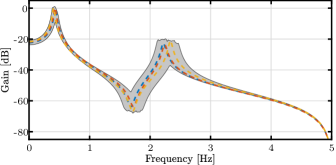
Figure 4: The FRFs during 100 Monte Carlo simulations are contained in ( ), where three FRFs are shown as ( , , ).

Additional simulation settings are seen in Table 1.

Table 1: Simulation settings.

Variable	Abbrevation	Value	Unit
Fast sampling time	$T_{h}$	0.1	s
Slow sampling time	$T_{l}$	0.3	s
Downsampling factor	$F$	3	-
Number of input samples	N	600	-
Number of output samples	M	200	-
Monte Carlo runs	-	100	-

Independent training and validation data sets are generated, where the excitation signals $u_{h}$ are random phase multisines with the same flat amplitude spectrum but different phase realizations. The output of the training set is disturbed with additive white Gaussian noise for $e_{h}$, where the signal-to-noise ratio, that is the ratio between the variance of $y_{h}$ and $e_{h}$, is randomly chosen in $\mathbb{R}_{[40,\>60]}$.

The following models are estimated using training data and compared on validation data in each Monte Carlo run.

• Unregularized least-squares FIR from (16) of order $P\in\mathbb{Z}_{[50,N]}$.

• Kernel regularized FIR using (18) of order $P\in\mathbb{Z}_{[50,N]}$, which uses the DC kernel $k_{DC}$ (22).

• Kernel regularized FIR using (18) of order $P\in\mathbb{Z}_{[50,N]}$, which uses the kernel function with prior knowledge from (24), specifically

  $$k_{PK}(i,j)=k_{DC}(i,j)+\sum_{n=1}^{2}k_{pk,n}(i,j).$$ (27)

The hyperparameters of the kernel regularized estimators are chosen as

$$\lambda =1, \omega_{1} =0.4T_{h}\cdot 2\pi, \omega_{2} =2T_{h}\cdot 2\pi,$$

$$\alpha =e^{-1.2T_{h}}, \alpha_{1} =\alpha_{2}=e^{-0.5T_{h}}, \gamma =10^{-5},$$

$$\beta =e^{-0.3T_{h}}, \sigma_{1,n} =\sigma_{2,n}=1,$$

where $\gamma_{1,n}$ and $\gamma_{2,n}$ are determined using (25). Additionally, the regularization parameter $\gamma$ and the hyperparameters $\omega_{n}$ and $\alpha_{n}$ are optimized using marginal likelihood optimization (26) with a gradient-based constrained optimizer to further enhance accuracy.

5.2 Simulation Results

For each Monte Carlo run, the Goodness of Fit (GoF) of the fast-rate output $y_{h}$ on the validation data is calculated,

$$\text{GoF}=100\left(1-\frac{\sum_{n=0}^{N-1}\left(y_{h,v}(n)-\hat{y}_{h}(n)\right)^{2}}{\sum_{n=0}^{N-1}\left(y_{h,v}(n)-\bar{y}_{h,v}\right)^{2}}\right),$$ (28)

where $\hat{y}_{h}$ is estimated using the fast-rate FIR models, $y_{h,v}(n)$ are the validation values, and $\bar{y}_{h,v}$ is the mean value of $y_{h,v}(n)$. The mean plus and minus 2 times its sample standard deviation over the Monte Carlo runs are seen in Figure 5.

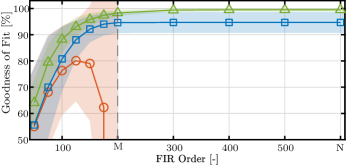
Figure 5: Kernel regularized estimators using DC kernel (22) ( ) or prior knowledge kernel (27) ( ) are capable of achieving a higher GoF for all model orders compared to least-squares FIR models ( ). In addition, the mean GoF $\pm 2$ times its sample standard deviation (shaded areas) show that the prior knowledge kernel decreases variance.

Additionally, the fast-rate FRFs have been evaluated for one Monte Carlo run, and are seen in Figure 6.

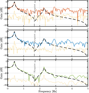
Figure 6: The regularized FIR models accurately identify the true FRF ( ) using a DC kernel ( ) (middle) and prior knowledge kernel ( ) (bottom), as shown by their low scaled FRF error $0.1\cdot\left|G_{0}\left(e^{j\omega_{k}T_{h}}\right)-G\left(e^{j\omega_{k}T_{h}}\right)\right|$ ( ). In contrast, the least-squares FIR model of order $P=150$ ( ) (top) fails to accurately identify the true FRF and has a high scaled FRF error ( ).

The following observations are made from the simulation results.

• From the GoF in Figure 5, the following is observed.

  • The least-squares FIR model is capable of estimating a model of order $P<M$, but not for $P>M$, supporting Lemma 1.

  • The kernel regularized FIR model with DC kernel accurately identifies models with low variance for all $P\in\mathbb{Z}_{[50,N]}$, due to the additional prior that is encoded in the estimator.

  • By adding the prior knowledge kernel to the regularized FIR estimate, the mean GoF is further increased from 94.67% to 99.5%, with significantly reduced variance for model orders $P>200$.

• From the FRFs in Figure 6, the following is observed.

  • The FRF of the least-squares FIR model with $P=150$ in the top doesn’t identify the FRF accurately, especially beyond the Nyquist frequency.

  • The FRF of the regularized FIR models in the middle and bottom are significantly more accurate with lower FRF error, especially beyond the Nyquist frequency of the slow-rate output.. In particular, the FIR model with prior knowledge kernel (bottom) accurately identifies the resonant behavior.

6 Experimental Validation

In this section, the developed method is validated using an experimental prototype wafer stage with slow-rate output, contributing to contribution C3.

6.1 Experimental Setup

The experimental setup is the prototype wafer stage in Figure 7 [24], which is used in semiconductor manufacturing and a prime example of mechatronic systems with slow-rate outputs.

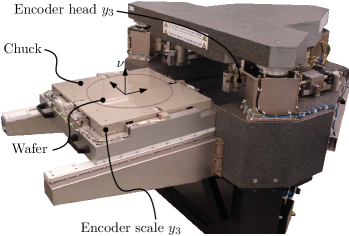
(a) Photograph of experimental setup.

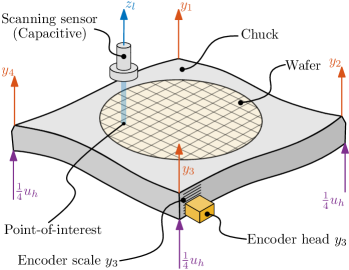
(b) Schematic overview of experimental setup.

Figure 7: Prototype experimental wafer stage setup used in semiconductor manufacturing with slow-rate output.

The objective of the wafer stage is to accurately control the vertical displacement $\nu$ of the point-of-interest on the wafer shown in Figure 7(a), which is the point on the wafer during lithographic exposure. The chuck and wafer are levitated, and actuated by four Lorentz actuators. The vertical displacement of the chuck is measured by four linear encoders and used as inputs to the feedback controller as $y=\frac{1}{4}\left(y_{1}+y_{2}+y_{3}+y_{4}\right)$. Directly measuring the vertical displacement of the point-of-interest on the wafer $\nu$ is not possible using linear encoders. The chuck of the wafer stage has internal lightly-damped structural modes. Consequently, measuring the vertical displacement on the outside of the chuck does not coincide with the vertical displacement at the wafer’s point of interest [25, 26]. Therefore, an external capacitive sensor, denoted by scanning sensor in Figure 7(b), directly measures the vertical displacement of the point-of-interest. The external capacitive sensor is sampled at a reduced sampling rate compared to the actuators, resulting in a slow-rate output.

6.2 Identification Setting

For this experimental validation, the goal is to identify the fast-rate equivalent model of the prototype wafer stage

$$G_{z}\left(q,\theta\right)=P_{z}\left(\vphantom{P_{y}\left(q,\theta\right)}q,\theta\right)\left(I+C\left(q\right)P_{y}\left(q,\theta\right)\right)^{-1}:u_{h}\mapsto z_{h},$$ (29)

using the fast-rate excitation $u_{h}$ and slow-rate outputs $z_{l}$. The prototype wafer stage is operating in closed-loop control, where the control structure is seen in Figure 8.

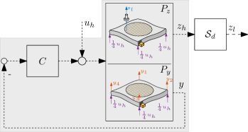
Figure 8: Experimental feedback scheme used, where the equivalent system in (29) is to be identified.

For this experimental validation, the fast-rate excitation signal $u_{h}$ is equally distributed over the four actuators, and is considered a disturbance to the plant. The excitation signal $u_{h}$ is a random noise sequence with flat amplitude spectrum, resulting in a signal-to-noise ratio of approximately 45 dB. The scanning sensor is suspended above the wafer, and is positioned in the bottom left corner of the wafer, 110 mm in both directions from the center. The experimental settings are seen in Table 2.

Table 2: Experimental settings.

Variable	Abbr.	Value	Unit
Fast sampling time	$T_{h}$	0.5	ms
Slow sampling time	$T_{l}$	1.5	ms
Downsampling factor	$F$	3	-
Number of input samples	N	600	-
Number of output samples	M	200	-

Similar to Section 5, FIR models are identified using unregularized and regularized least-squares cost functions, i.e., the following methods are compared.

• Unregularized least-squares FIR from (16) of order $P\in\mathbb{Z}_{[5,N]}$.

• Kernel regularized FIR using (18) of order $P\in\mathbb{Z}_{[5,N]}$, which uses the DC kernel $k_{DC}$ (22).

• Kernel regularized FIR using (18) of order $P\in\mathbb{Z}_{[5,N]}$, which uses the kernel function with prior knowledge from (24), specifically

  $$k_{PK}(i,j)=k_{DC}(i,j)+\sum_{n=1}^{3}k_{pk,n}(i,j).$$ (30)

The hyperparameter of the kernels are initialized as

$$\lambda =1, \alpha =\alpha_{n}=e^{-80T_{h}},$$

$$\omega_{1} =490T_{h}\cdot\!2\pi \omega_{2} =510T_{h}\cdot\!2\pi, \omega_{3} =870T_{h}\cdot\!2\pi,$$

$$\beta =e^{-20T_{h}}, \sigma_{1,n} =\sigma_{2,n}=1, \gamma =10^{-1}$$

where $\gamma_{1,n}$ and $\gamma_{2,n}$ are determined using (25). The hyperparameters $\omega_{n}$ and $\alpha_{n}$ are refined using a gradient based constrained optimizer for the marginal likelihood (26).

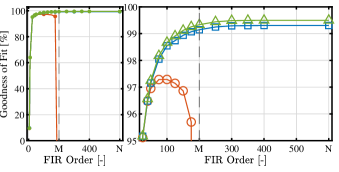
Figure 9: The GoF of the regularized FIR models with DC kernel (22) ( ) and prior knowledge kernel (30) ( ) are higher compared to the unregularized least-squares FIR model ( ) for all model orders $P\in\mathbb{Z}_{[5,N]}$ (left) and $P\in\mathbb{Z}_{[25,N]}$ (right).

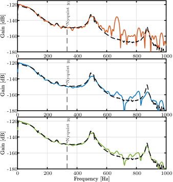
(a) The validation FRF $G_{0}\left(e^{j\omega_{k}T_{h}}\right)$ (31) ( ) is estimated accurately by regularized FIR models with DC kernel ( ) and prior knowledge kernel ( ), in contrast to the least-squares FIR model ( ).

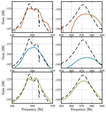
(b) Enlarged sections of the resonant behavior around 500 Hz (left) and 870 Hz (right) show that the FIR model with prior knowledge kernel accurately identifies the resonant behavior compared to the validation FRF $G_{0}\left(e^{j\omega_{k}T_{h}}\right)$ (31).

Figure 10: The regularized FIR models accurately identify the validation FRF $G_{0}\left(e^{j\omega_{k}T_{h}}\right)$ (31) of the prototype wafer stage ( ) using a DC kernel ( ) (middle) and prior knowledge kernel ( ) (bottom). In contrast, the least-squares FIR model of order $P=100<M$ ( ) (top) fails to accurately identify the validation FRF.

For validation purposes, the fast-rate outputs $z_{h}$ are recorded as well, and a validation data set with similar signal-to-noise ratio is created to compare the approaches. Finally, another data set is created where the fast-rate outputs $z_{h}$ are recorded as well, which is used to identify a validation FRF

$$G_{0}\left(e^{j\omega_{k}T_{h}}\right):\frac{U_{h}\left(e^{j\omega_{k}T_{h}}\right)}{\vphantom{U_{h}\left(e^{j\omega_{k}T_{h}}\right)}Z_{h}\left(e^{j\omega_{k}T_{h}}\right)}.$$ (31)

This validation FRF is identified with the local rational modeling method from McKelvey2012 [27], using local rational degrees $R=4$, local window size $n_{w}=150$, and $50000$ samples.

6.3 Experimental Results

The GoF in (28) for the validation data set is shown for various model orders in Figure 9. The estimated FRFs are seen in Figure 10, including an enlarged section of the resonant behavior around 500 and 870 Hz.

The following observations are made with respect to the experimental results.

• From the GoF in Figure 9, the following is observed.

  • The GoF for the regularized FIR model estimates using either the DC or prior knowledge kernel is high for all model orders, close to 100% for $P\to N$.

  • The GoF for the least-squares FIR model estimates is significantly lower, and is not capable of estimating a model for $P>M$.

  • The regularized FIR model with prior knowledge kernel and $P=N$ achieves a GoF of 99.44%, and a root-mean-squared error of

    $$\sqrt{\frac{1}{N}\sum_{n=0}^{N-1}\left(y_{h,\nu}(n)-\hat{y}_{h}(n)\right)}=1.65\times 10^{-8}\text{ m}.$$

    In comparison, the least-squares FIR model with highest GoF 97.29% has a root-mean-squared error of $3.62\times 10^{-8}$ m, which is more than double.

• From the FRFs in Figure 10, the following is observed.

  • Both the regularized FIR models with DC kernel and prior knowledge kernel estimate the FRF accurately with little noise, even beyond the Nyquist frequency of the slow-rate output.

  • The resonant behavior at 500 and 870 Hz in Figure 10(b) is estimated accurately by the regularized FIR model with prior knowledge kernel, which is explained by the additional prior information that is introduced.

  • The least-squares FIR model is not capable of estimating the FRF accurately, including the resonant dynamics. Furthermore, it introduces several artificial resonances, especially around $f_{l}=666\frac{2}{3}$ Hz, which is caused by aliasing of the gain around 0 Hz to this frequency.

7 Conclusions

The results in this paper determine conditions for unique identification of reduced-order FIR models and arbitrary order fast-rate models for systems with slow-rate output measurements, including non-parametric models, and additionally enables intersample response estimation. The method incorporates generic prior information through kernel regularization, that determines arbitrary order fast-rate models. This enables the usage of prior knowledge kernels that encode information about the poles of a system, resulting in a method which is highly suitable for lightly-damped systems.

The framework is validated using a Monte Carlo simulation example, which shows that the regularized FIR models have increased estimation quality and decreased variance. Furthermore, the framework is validated on a prototype wafer stage with a slow-rate output, showing that the regularized FIR models are capable of estimating the system, including lightly-damped resonant dynamics. The developed approach is a key enabler for control design of systems with slow-rate output measurements.

References

- [1] H. Fujimoto, Y. Hori, Visual Servoing Based on Multirate Control and Dead-time Compensation, Journal of the Robotics Society of Japan 22 (6) (2004) 780–787. https://doi.org/10.7210/jrsj.22.780.
- [2] N. Sivashankar, P. Khargonekar, Robust stability and performance analysis of sampled-data systems, IEEE Transactions on Automatic Control 38 (1) (1993) 58–69. https://doi.org/10.1109/9.186312.
- [3] T. Chen, B. A. Francis, Optimal Sampled-Data Control Systems, Springer, 1995. https://doi.org/10.1007/978-1-4471-3037-6.
- [4] D. Li, S. L. Shah, T. Chen, Analysis of dual-rate inferential control systems, Automatica 38 (6) (2002) 1053–1059. https://doi.org/10.1016/S0005-1098(01)00295-3.
- [5] M. Cech, A.-J. Beltman, K. Ozols, Digital Twins and AI in Smart Motion Control Applications, in: 2022 IEEE 27th International Conference on Emerging Technologies and Factory Automation (ETFA), IEEE, 2022, pp. 1–7. https://doi.org/10.1109/ETFA52439.2022.9921533.
- [6] R. M. Schmidt, G. Schitter, A. Rankers, J. van Eijk, The design of high performance mechatronics, Delft University Press, 2020. https://doi.org/10.3233/STAL9781643680514.
- [7] R. Pintelon, J. Schoukens, System Identification: A Frequency Domain Approach, John Wiley & Sons, 2012.
- [8] T. Söderström, P. Stoica, System Identification, Prentice Hall, 1989.
- [9] L. Ljung, System Identification: Theory for the User, Prentice Hall, 1998.
- [10] L. Ljung, T. Chen, B. Mu, A shift in paradigm for system identification, International Journal of Control 93 (2) (2020) 173–180. https://doi.org/10.1080/00207179.2019.1578407.
- [11] G. Pillonetto, F. Dinuzzo, T. Chen, G. De Nicolao, L. Ljung, Kernel methods in system identification, machine learning and function estimation: A survey, Automatica 50 (3) (2014) 657–682. https://doi.org/10.1016/j.automatica.2014.01.001.
- [12] H. Unbehauen, G. Rao, Continuous-time approaches to system identification—A survey, Automatica 26 (1) (1990) 23–35. https://doi.org/10.1016/0005-1098(90)90155-B.
- [13] L. Ljung, Experiments with Identification of Continuous Time Models, in: Proceedings of the 15th IFAC Symposium on System Identification, 2009, pp. 1175–1180. https://doi.org/10.3182/20090706-3-FR-2004.00195.
- [14] F. Ding, T. Chen, Identification of dual-rate systems based on finite impulse response models, International Journal of Adaptive Control and Signal Processing 18 (7) (2004) 589–598. https://doi.org/10.1002/acs.820.
- [15] Y. Zhu, H. Telkamp, J. Wang, Q. Fu, System identification using slow and irregular output samples, Journal of Process Control 19 (1) (2009) 58–67. https://doi.org/10.1016/j.jprocont.2008.02.002.
- [16] D. Li, S. L. Shah, T. Chen, Identification of fast-rate models from multirate data, International Journal of Control 74 (7) (2001) 680–689. https://doi.org/10.1080/00207170010018904.
- [17] J. Ding, F. Ding, X. P. Liu, G. Liu, Hierarchical Least Squares Identification for Linear SISO Systems With Dual-Rate Sampled-Data, IEEE Transactions on Automatic Control 56 (11) (2011) 2677–2683. https://doi.org/10.1109/TAC.2011.2158137.
- [18] M. van Haren, L. Mirkin, L. Blanken, T. Oomen, Beyond Nyquist in Frequency Response Function Identification: Applied to Slow-Sampled Systems, IEEE Control Systems Letters 7 (2023) 2131–2136. https://doi.org/10.1109/LCSYS.2023.3284344.
- [19] J. Lataire, T. Chen, Transfer function and transient estimation by Gaussian process regression in the frequency domain, Automatica 72 (2016) 217–229. https://doi.org/10.1016/j.automatica.2016.06.009.
- [20] N. Hallemans, R. Pintelon, B. Joukovsky, D. Peumans, J. Lataire, FRF estimation using multiple kernel-based regularisation, Automatica 136 (2022) 110056. https://doi.org/10.1016/j.automatica.2021.110056.
- [21] L. Ljung, T. Glad, On global identifiability for arbitrary model parametrizations, Automatica 30 (2) (1994) 265–276. https://doi.org/10.1016/0005-1098(94)90029-9.
- [22] T. Oomen, J. van de Wijdeven, O. Bosgra, Suppressing intersample behavior in iterative learning control, Automatica 45 (4) (2009) 981–988. https://doi.org/10.1016/j.automatica.2008.10.022.
- [23] A. N. Tikhonov, V. Y. Arsenin, Solutions of ill-posed problems, John Wiley & Sons, 1977.
- [24] K. Classens, J. van de Wijdeven, M. Heemels, T. Oomen, From Fault Diagnosis and Predictive Maintenance to Control Reconfiguration, Mikroniek (5) (2023) 5–12.
- [25] T. Oomen, E. Grassens, F. Hendriks, Inferential Motion Control: Identification and Robust Control Framework for Positioning an Unmeasurable Point of Interest, IEEE Transactions on Control Systems Technology 23 (4) (2015) 1602–1610. https://doi.org/10.1109/TCST.2014.2371830.
- [26] M. Heertjes, H. Butler, N. Dirkx, S. van der Meulen, R. Ahlawat, K. O’Brien, J. Simonelli, K.-T. Teng, Y. Zhao, Control of Wafer Scanners: Methods and Developments, in: Proceedings of the IEEE American Control Conference (ACC), 2020, pp. 3686–3703. https://doi.org/10.23919/ACC45564.2020.9147464.
- [27] T. McKelvey, G. Guérin, Non-parametric frequency response estimation using a local rational model, in: Proceedings of the 16th IFAC Symposium on System Identification, 2012, pp. 49–54. https://doi.org/10.3182/20120711-3-BE-2027.00299.